Article

Research on Trajectory Tracking Control of USV Based on Disturbance Observation Compensation

School of Shipbuilding and Ocean Engineering, Jiangsu University of Science and Technology, Zhenjiang 212003, China
*
Author to whom correspondence should be addressed.
J. Mar. Sci. Eng. 2026, 14(8), 757; https://doi.org/10.3390/jmse14080757
Submission received: 1 April 2026 / Revised: 19 April 2026 / Accepted: 20 April 2026 / Published: 21 April 2026
(This article belongs to the Section Ocean Engineering)

Abstract

To address trajectory-tracking degradation of unmanned surface vehicles (USVs) in constrained waters caused by model uncertainty, strong environmental disturbances, and actuator limitations, this paper proposes a robust disturbance-observer-based optimization model predictive control method. First, a nonlinear tracking error model is established for a 3-DOF USV by incorporating environmental loads, parametric perturbations, and unmodeled dynamics into the kinematic and dynamic equations. Based on this model, a prediction model suitable for model predictive control is derived through linearization and discretization. Then, to estimate complex unknown disturbances online, a robust disturbance observer integrating a radial basis function neural network (RBFNN) with an adaptive sliding-mode mechanism is developed, enabling real-time approximation and compensation of lumped disturbances in the surge and yaw channels. Furthermore, to overcome actuator saturation caused by the direct superposition of feedforward compensation and feedback control in conventional composite strategies, a dynamic constraint reconstruction mechanism is introduced. By feeding the observer-generated compensation signal back into the MPC optimizer, the feasible control region is updated online so that the total control input satisfies both magnitude and rate constraints of the propulsion system. Theoretical analysis based on Lyapunov theory proves the uniform ultimate boundedness of the observation errors and neural-network weight estimation errors, while input-to-state stability theory is employed to establish closed-loop stability. Comparative simulations under sinusoidal trajectories, time-varying curvature paths, and large-maneuver turning conditions demonstrate that the proposed method significantly improves tracking accuracy, disturbance rejection capability, and control feasibility under severe disturbances and parameter mismatch.

1. Introduction

With the rapid development of fields such as marine resource exploitation, environmental monitoring and military reconnaissance [1], Unmanned Surface Vehicles (USVs) have become the core carriers for marine mission execution due to their high autonomy, wide operation range and strong risk avoidance ability. According to statistics from the International Maritime Organization, the global unmanned vessel market size exceeded 5 billion US dollars in 2024, of which over 60% was attributed to the demand for precise path planning and tracking in restricted waters [2]. However, the restricted water area has limited horizontal maneuverability, which leads to three challenges for traditional path tracking methods: model uncertainty, disturbance sensitivity and real-time constraints. Traditional control methods have difficulty simultaneously satisfying the requirements of high-precision tracking and strong robustness. There is a clear need to explore new control strategies to enhance the autonomous navigation ability of USVs under complex working conditions [3].
Trajectory tracking control strategies can generally be categorized into the following types: classical geometry-based methods such as Pure Pursuit and the Stanley algorithm; control methods based on vehicle dynamic models, including Linear Quadratic Regulator (LQR) and Model Predictive Control (MPC); and data-driven and intelligent control approaches, such as Reinforcement Learning (RL) and Deep Neural Networks (DNNs) [4,5]. Model Predictive Control (MPC) has become mainstream due to its multi-objective optimization and constraint processing capabilities [6]. Existing studies show that MPC can predict future states through rolling optimization and achieve centimeter-level tracking accuracy in a static environment. However, the uncertainty of ship dynamics parameters and environmental disturbances in actual waters can lead to a mismatch with the nominal model of the MPC, significantly reducing the control performance. Many scholars have conducted research to improve MPC. Raffo GV et al. proposed a model predictive controller (MPC) structure, considering both kinematic and dynamic control simultaneously. The research includes a comparative study between two kinematic linear predictive control strategies: The first strategy is based on the concept of continuous linearization, and the other strategy combines a local reference frame with an approach path strategy [7]. Wang H et al. proposed an improved model predictive control (MPC) controller based on fuzzy adaptive weight control to solve the problem of autonomous vehicle in the process of path tracking caused by the application of the classical MPC controller when the vehicle deviates from the target path [8]. Ostafew CJ et al. introduced a nonlinear model predictive control (RC-LB-NMPC) algorithm based on robust constraint learning for path tracking in off-road terrain [9]. Backman J et al. derived a nonlinear model predictive path tracking approach for tractor and trailer systems [10]. Zhou et al. designed a heading tracking redundant on Model Predictive Control (MPC). A mathematical model of ship motion under wind and wave disturbance was established. The designed MPC heading tracking control algorithm shows good accuracy for tracking waypoints [11]. B. Zhao et al. proposed an improved model predictive control (MPC) based on global heading constraint (GCC) and event-triggered mechanism (ETM) to address the path tracking problem of unmanned surface vessels (USVs). The designed GCC guidance law combines a LOS concept and overcomes the problem of the lack of reference signals near the waypoints. The developed MPC controller involves ETM, which minimizes the deviation based on its predictive ability and energy-saving effect [12]. Luo Q et al. [13] proposed a model based on model-free Extended State Observer (MFESO) and a model-free predictive control (MPC-MFESO-MFPAC) method to achieve trajectory tracking and obstacle avoidance of unmanned surface vehicles (USVs) in complex environments. The reverse step method is adopted to eliminate the rotational characteristics, enabling MFPAC to be directly applied to USV control. Zhao S et al. introduced fractional model predictive control (FOMPC) for USV heading control within the framework of Extended Predictive Adaptive Control (EPSAC) [14]. Li A et al. proposed a path tracking control method based on Model Predictive Static Programming (MPSP) for unmanned surface vessels (USVs) subject to input disturbance. This method addresses the challenges of accurate USV dynamic modeling, unpredictable marine environments, and limited power and energy systems [15]. Zhang L et al. proposed an adaptive model predictive control (MPC) method based on the Actor–Critic (AC) reinforcement learning (RL) strategy. This combines MPC with AC RL to continuously adjust the state weight coefficients in the model predictive controller to solve the problem of increased error caused by poor control parameters [16]. Despite these advances, conventional composite control strategies typically superimpose disturbance compensation directly onto the feedback control law. If the physical limitations of the propeller and rudder are neglected, this approach can easily lead to actuator saturation, control interruption, and even instability of the closed-loop system.
In recent years, several advanced constrained control strategies have been reported for marine vehicles, including Tube MPC, Robust MPC, and observer-based MPC frameworks such as ESO-based MPC. Tube MPC and Robust MPC improve robustness mainly through bounded uncertainty modeling, invariant tube design, or conservative constraint tightening [17]. Observer-based MPC methods, on the other hand, improve control performance by estimating disturbances online and introducing feedforward compensation. However, for constrained USV systems operating under strongly nonlinear and state-dependent marine disturbances, the interaction between disturbance compensation and actuator-constrained optimization is still not sufficiently addressed. In particular, many existing methods do not explicitly update the admissible control region according to the compensation demand. This motivates the compensation-aware dynamic constraint reconstruction strategy proposed in this work.
Although disturbance-observer-based MPC, neural-network-assisted compensation, and sliding-mode-enhanced control have all been investigated in the literature, the present work differs from existing studies in the following aspects.
(1)
Instead of directly superimposing disturbance compensation onto the feedback control law as in many conventional composite strategies, this paper develops an RDO-MPC framework in which the observer-generated compensation signal is simultaneously used for feedforward disturbance rejection and for online reconstruction of the admissible MPC constraint set. This coupling explicitly accounts for actuator saturation and preserves the physical feasibility of the total control input.
(2)
To address the state-dependent and time-varying nature of marine disturbances, an RBFNN-based adaptive robust disturbance observer is designed. In contrast to fixed-bound sliding-mode compensation or purely linear disturbance estimation, the proposed observer combines online neural approximation of lumped disturbances with robust sliding-mode correction, thereby improving adaptability to nonlinear uncertainties while suppressing excessive chattering.
(3)
The proposed method emphasizes the coordinated realization of disturbance rejection, constraint handling, and trajectory-tracking optimization under actuator limitations. Therefore, the contribution of this work lies not only in improving tracking accuracy, but also in establishing a compensation-aware optimization framework that better matches the practical requirements of constrained USV propulsion systems.
The remainder of this paper is organized as follows: Section 2 describes the kinematics and disturbance-inclusive dynamic models of the USV, and derives the nonlinear error dynamic equations utilized for the controller design. Section 3 specifies design framework of the RDO-MPC controller. This primarily includes the construction of the nominal Robust Model Predictive Controller (RMPC), the design of the RBFNN-based adaptive robust disturbance observer, the synthesis of the composite control law, and the stability analysis of the closed-loop system. Section 4 outlines the setup for the numerical simulation experiments and verifies the effectiveness, superiority, and robustness of the proposed algorithm through comparative tests under various complex path and sea state conditions. Section 5 summarizes the conclusions of this research.

2. Theoretical Foundations and Problem Formulation

2.1. Kinematic and Dynamic Models of USVs

In USV path tracking applications, USV position and heading are key concerns. The USV mathematical model is divided into kinematic and dynamic models. The kinematic model is used to describe the motion state of the USV, while the dynamic model is used to simulate the relationship between the force and acceleration of the hull through physical laws and mathematical equations, providing a theoretical basis for design, control and optimization. Under normal circumstances, the motion and control problem of USV is simplified to three degrees of freedom to describe the motion of USV in the plane. In USV trajectory-tracking applications, the position, heading, and planar velocity states are of primary concern. Following the notation of Fossen [18], the motion of the USV is simplified to a three-degree-of-freedom planar model. Table 1 shows the physical parameters and dynamic model coefficients of the unmanned surface vessels used in this study, which were all derived from the “Explorer” platform independently developed by our laboratory. These include design specifications, measured platform data, and model settings used for simulation. As shown in Figure 1, two coordinate frames are introduced, namely the inertial frame o n x n y n and the body-fixed frame o b x b y b . The position and heading variables in the inertial frame are denoted by η = x , y , ψ T , where x and y represent the position coordinates and ψ denotes the heading angle. The velocity vector in the body-fixed frame is denoted by v = u , v , r T , where u , v and r . represent the surge velocity, sway velocity, and yaw rate, respectively. Figure 1a shows the physical configuration and body-fixed motion directions of the USV, while Figure 1b illustrates the coordinate definitions and motion variables used in the mathematical model. Therefore, its kinematic model can be expressed as follows:
η ˙ = R ψ v .
In Equation (2), R ψ is the transformation matrix for converting the velocity vectors between the body- fixed frame and the inertial frame, denoted as follows:
R ψ = cos ψ sin ψ 0 sin ψ cos ψ 0 0 0 1 .
Considering the speed restrictions applying in constricted areas such as inland lakes or ports, the dynamic model of USV can be expressed as follows:
M v ˙ + C v v + D v v = τ + τ d i s t ,
In Equation (3), M = M R B + M A is the generalized mass matrix (including the rigid body mass M R B and the added mass M A ), which describes the acceleration behaviour of the USV on the water surface, denoted as follows:
M = m X u ˙ 0 0 0 m Y v ˙ m x g Y r ˙ 0 m x g N v ˙ I z z N r ˙ .
In Equation (3), the Coriolis matrix C v can be decomposed as follows:
C v = C R B v + C A v ,
In Equation (5), C R B v is the term for rigid body motion, and C A v is the added mass term of fluid motion. The coupling effect caused by the added mass is expressed using Newtonian mechanics:
C R B ( v ) = [ 0 0 m ( y g r + v ) 0 0 m ( x g r u ) m ( y g r + v ) m ( x g r u ) 0 ] ,
C A v = 0 0 Y v ˙ v + Y r ˙ r 0 0 X u ˙ u Y v ˙ v Y r ˙ r X u ˙ u 0 .
In Equation (3), the damping matrix D v represents hydrodynamic dissipative effects, which can be decomposed into:
D v = D L + D Q v ,
In Equation (8), D L is the linear damping matrix and D Q v is the quadratic damping matrix. They are, respectively, expressed as follows:
D L = X u 0 0 0 Y v Y r 0 N v N r ,
D Q ( v ) = [ X u | u | | u | 0 0 0 Y v | v | | v | + Y v | r | | r | Y r | v | | v | + Y r | r | | r | 0 N v | v | | v | + N v | r | | r | N r | v | | v | + N r | r | | r | ] .
In Equation (10), the diagonal terms X u , Y v , N r dominate the linear attenuation of the longitudinal/transverse/forecasted motion; non-diagonal item Y r , N v represent damping of lateral and forward motion. The diagonal term X u u , Y v v , N r r is proportional to the square of the velocity, The cross term Y r v , N v r describes the secondary coupling of the lateral and forward motion. These equations are approximations that retain only the most important hydrodynamical effects.
The control input τ is generated by two thrusters. Let τ = τ u , τ v , τ r T denote the thrust force and moment vectors of the unmanned surface vessel, respectively, where τ u represents the surge force, τ v represents the sway force and τ r represents the yaw moment. The following equation describes the resultant forces and moment generated by the two thrusters:
τ = τ u τ v τ r = T p o r t cos θ + T s t b d cos δ T p o r t sin θ + T s t b d sin δ T s t b d sin δ T p o r t sin θ × B d / 2 ,
In Equation (11), T p o r t and T s t b d denote the thrusts generated by the left and right thrusters, respectively, while θ , δ represent the steering angles of the left and right vector rudders. The spacing B d between the two thrusters determines the yaw moment of the USV. A larger spacing results in a greater turning moment; however, it is constrained by the vessel beam. The distance between the two thrusters is typically about 45–60% of the vessel beam. Accordingly, the thruster spacing is selected as B d = 1.7 m. Magnitude constraints on thrust and moment are used to model the physical limits of the propeller rotational speed and rudder angle, whereas rate constraints are introduced to protect the mechanical structure and prevent excessive wear caused by abrupt control inputs. The actuator constraint parameters are listed in Table 2. The actuator limitation parameters are determined from the actual propulsion-system operating range and safety limits of the twin-thruster USV platform developed in our laboratory.
τ d i s t represents environmental disturbances, including complex flow fields in narrow waters and wake flows from adjacent vessels, etc. The environmental disturbance term can be modeled as follows:
τ d i s t = τ c + τ w i n d + τ w a v e ,
In Equation (12), τ c disturbance due to water flow (currents). A quasi-constant model is adopted and is proportional to the square of the relative velocity. τ w i n d , disturbance due to wind, is modeled based on the typical wind speed distribution at the port; τ w a v e , wave disturbance, considers the influence of short-period waves, where the amplitude decays with water depth, and the JONSWAP spectrum correction for short wave peak modeling in restricted waters [19]. Their respective expressions are:
τ c = X c Y c N c = 1 2 ρ a V c 2 C X c A u w cos γ c ψ 1 2 ρ a V c 2 C Y c A u w sin γ c ψ 1 2 ρ a V c 2 C N c A u w L sin 2 γ c ψ ,
τ w i n d = X w Y w N w = 1 2 ρ a V w 2 C X w A f w cos γ w ψ 1 2 ρ a V w 2 C Y w A s w sin γ w ψ 1 2 ρ a V w 2 C N w A s w L sin 2 γ w ψ ,
τ w a v e = X J Y J N J = ρ g 0 S ω C X J ω , d ω cos ψ 0 S ω C Y J ω , d ω sin ψ L 0 S ω C N J ω , d ω sin 2 ψ .
By incorporating the aforementioned disturbances into the 3-DOF dynamic equations of the USV, the extended form can be obtained as follows:
M v ˙ + C v v + D v v = τ + τ e n v .
Here, τ e n v = τ w i n d + τ w a v e + τ c denotes the total environmental disturbance vector, and its components represent the external disturbance forces acting on the USV in the three degrees of freedom. The inclusion of τ e n v = d u , d v , d r T makes the model more realistic; however, it also introduces additional nonlinearity and uncertainty, which may amplify path-following errors. In control design, the disturbance d u , d v , d r can be estimated and compensated using robust control methods or disturbance observers, thereby ensuring system stability. The environmental disturbance model established in this section provides a solid foundation for the subsequent validation of path-following control and multi-USV cooperative control algorithms, enhancing the realism of USV simulations.
Neglecting disturbances, the USV dynamics can be approximated as follows:
m + X u ˙ u ˙ m + Y v ˙ v r = τ u X u u X u u u u m + Y v ˙ v ˙ m + X u ˙ u r = τ v Y v v Y v v v v I z z + N r ˙ r ˙ Y v ˙ X u ˙ u v = τ r N r r N r r r r .

2.2. Coordinate System and Error Variable Description

The core objective of path-following control is to drive the USV to minimize position and heading errors with respect to the desired path. To implement the RDO-MPC composite control strategy proposed in this chapter, it is first necessary to derive a dynamic model with path-following errors as the state variables, based on the kinematic and dynamic equations established. In this section, a nonlinear tracking error model is first formulated. It is then reformulated into a control-affine nonlinear form suitable for sliding mode observer design [20]. Finally, the model is linearized and discretized to meet the requirements of the model predictive control (MPC) scheme.
To describe the path-following task, a virtual reference vessel moving along the predefined trajectory is introduced. The state vector of the reference trajectory is denoted by η d = x d , y d , ψ d T , and the corresponding reference velocity vector is denoted by v d = u d , v d , r d T .
The control objective of path-following is to drive the actual state η to converge to the reference state η d , i.e., as t , the tracking error η η d 0 approaches zero. Considering the underactuated nature of the USV and the physical meaning of the control inputs, the position error defined in the inertial frame is typically projected onto the object-fixed frame for representation. Accordingly, the path-following error vector ε = x e , y e , ψ e T can be defined as follows:
x e y e ψ e = R T ψ η η d = cos ψ sin ψ 0 sin ψ cos ψ 0 0 0 1 x x d y y d ψ ψ d ,
Here, x e , y e , and ψ e represent the longitudinal tracking error, lateral tracking error, and heading error in the object-fixed frame, respectively. Perfect tracking of the reference trajectory is achieved when ε 0 . The designed reference trajectory is feasible for practical USV implementation. Physical constraints of the USV have been explicitly considered and incorporated during trajectory generation, including continuous and smooth variations in speed and heading, as well as curvature in all turning segments that exceeds the USV’s minimum turning radius. The trajectory is compatible with the USV’s dynamic model, and the tracking controller ensures that the deviation of the actual path from the reference trajectory remains within a bounded range.

2.3. Derivation of Nonlinear Error Dynamic Equations

By taking the time t derivative of both sides of Equation (18) and combining it with the USV kinematic equations established, the nonlinear kinematic error differential equations for USV path-following can be obtained after simplification and rearrangement:
x ˙ e = u u d cos ψ e v d sin ψ e + r y e y ˙ e = v v d cos ψ e + u d sin ψ e r x e ψ ˙ e = r r d .
In underactuated USV path-following control, the lateral velocity v is typically assumed to be small, and the lateral velocity of the reference trajectory is often considered negligible. The above equation describes the geometric relationship between the position errors and the vessel’s velocity and heading.
Furthermore, by incorporating the disturbance-inclusive dynamic Equation (16), it follows that:
v ˙ = M 1 τ + τ e n v C v v D v v .
To facilitate the approximation of unmodeled dynamics and disturbances using a radial basis function (RBF) neural network in the subsequent section, the aforementioned kinematic error equations and dynamic equations are combined and reformulated into a unified control-affine nonlinear form.
The state variable is defined as X = x e , y e , ψ e , u , v , r T . Considering that the USV studied in this paper is underactuated, the control input is approximated by U = τ = τ u , 0 , τ r , where τ u , τ r represent the net surge thrust and yaw moment, respectively. Accordingly, the system state equation can be expressed as follows:
X ˙ = f X + g X U + d X , t ,
The specific definitions of each term in the above equation are given as follows: f X denotes the nominal drift vector field, which includes the kinematic coupling terms and the known components of the dynamic model:
f ( X ) = u u d cos ψ e + r y e v + u d sin ψ e r x e r r d M 11 1 ( d u u + m 22 v r ) M 22 1 ( d v v m 11 u r ) M 33 1 ( d r r + ( m 11 m 22 ) u v ) .
g X denotes the control input matrix, which characterizes the influence of the surge thrust τ u and yaw moment τ r on the system states:
g ( X ) = 0 0 0 0 0 0 1 / m 11 0 0 0 0 1 / m 33 .
d X , t denotes the lumped disturbance term, which incorporates environmental disturbances τ e n v , model parameter perturbations, and unmodeled higher-order nonlinear hydrodynamic effects. Due to its strong nonlinearity and uncertainty, d X , t will be approximated online using a RBFNN in the next section.

2.4. Model Linearization and Discretization for MPC

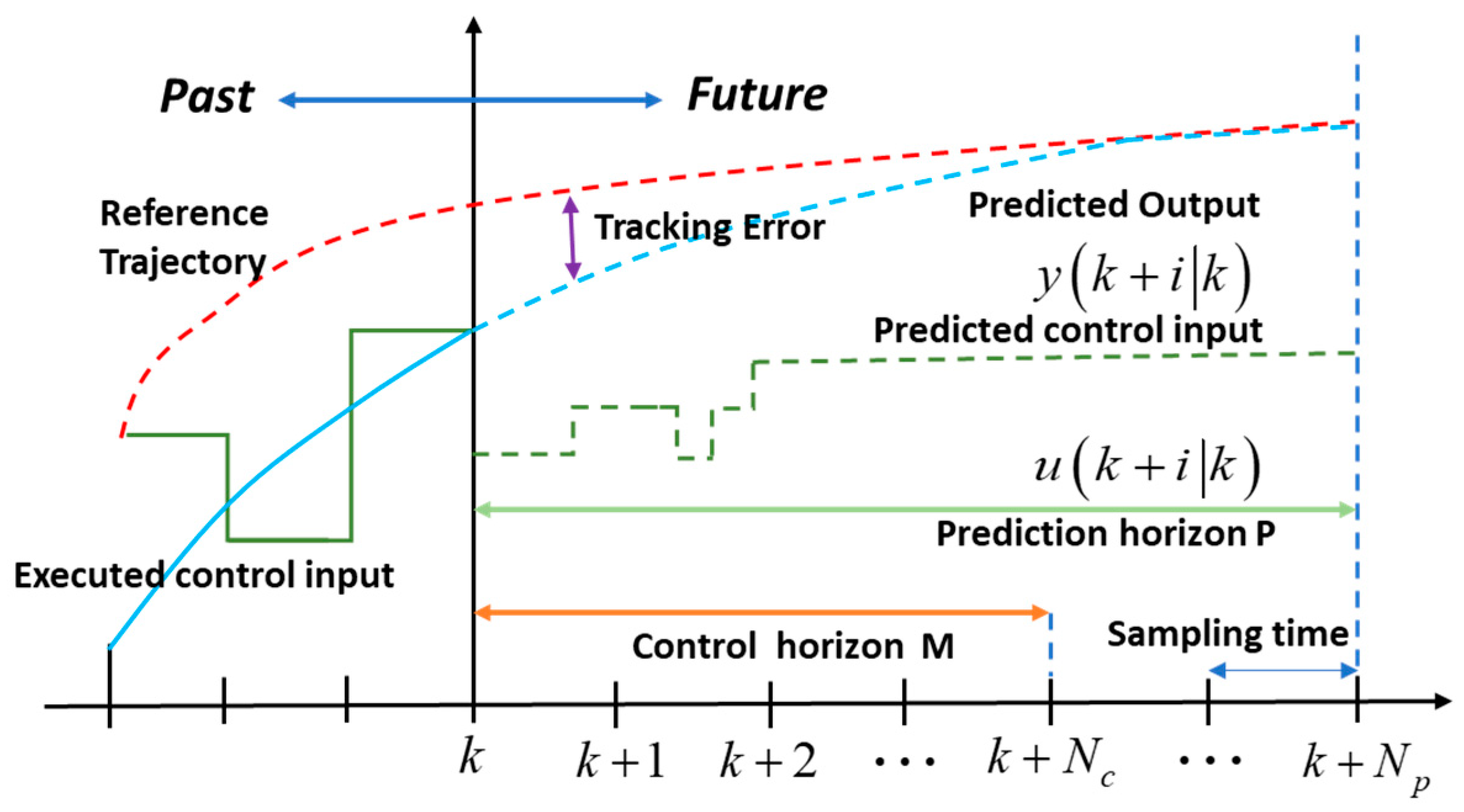
MPC is an advanced control strategy based on rolling optimization and feedback correction. Its core idea is to achieve real-time control of multi-constraint and multi-objective systems by solving optimization problems in a finite time domain online. The basic schematic diagram of MPC is shown in Figure 2: At time step k , the future system behavior over a prediction horizon of length P is optimized in a receding-horizon manner based on the current system state and the prediction model. The controller generates a future control sequence by solving an optimization problem that includes tracking errors and control input constraints, but only executes the optimal control quantity at the current moment. As time progresses to the next sampling point, the system provides real-time feedback on the actual output, re-conducts prediction and optimization, and forms a closed loop of ‘prediction—execution—correction’. This mechanism enables the MPC to dynamically adapt to system changes and take into account the complex requirements of multivariable systems by proactively balancing tracking accuracy and control costs, while explicitly handling physical constraints.
Since conventional MPC algorithms rely on linear models for receding-horizon optimization, directly handling the aforementioned nonlinear model would result in excessive computational burden and make it difficult to ensure real-time performance. Therefore, it is necessary to linearize the system around the reference trajectory points [21].
Assume that the reference trajectory corresponds to the reference state X r e f and control input U d = τ u d , 0 , τ r d T , which serve as the equilibrium operating point. By performing a Taylor series expansion around the equilibrium point X ˙ = f X , U and neglecting higher-order terms, the continuous-time linear time-varying state-space equations can be obtained.
X ˜ ˙ = A t X ˜ + B t U ˜ + d ω t ,
Here, X ˜ = X X r e f and U ˜ = U U d denote the state and control input, respectively, while d ω t represents the disturbance term arising from linearization residuals and external environmental disturbances. In the MPC prediction model, d ω t is typically neglected or assumed to be a constant disturbance. The resulting modeling error is compensated in the closed-loop control by a sliding mode observer. The matrices A t , B t denote the Jacobian matrices with respect to the state and input, respectively, defined as follows:
A t = f x | X r e f , U d , B t = f u | X r e f , U d .
To facilitate the implementation of the MPC algorithm in a digital control framework, a sampling time T s is defined, and the continuous-time state-space model is discretized using the Euler method as follows:
A k = I + T s × A t B k = T s × B t .
Finally, the discrete-time linear state-space model for the MPC controller design is obtained as follows:
X k + 1 = A k X k + B k U k .
This equation describes the evolution of the USV states with respect to the control inputs under ideal disturbance-free conditions, and serves as the basis for multi-step receding-horizon prediction in MPC.

3. Design of Robust MPC Controller Based on Disturbance Observation Compensation

3.1. Design of Robust Model Predictive Controller

In the composite control scheme proposed in this chapter, the RMPC serves as the primary controller. Its main objective is to compute the optimal control input sequence based on the nominal system model, while satisfying the physical actuator constraints of the USV, in order to achieve accurate tracking of the reference trajectory. Considering that the error model established in the previous section has been linearized and that model mismatch inevitably exists in practical navigation, directly applying a standard MPC strategy is insufficient to eliminate steady-state errors. Therefore, the RMPC controller designed in this section focuses on handling the nominal system dynamics, while the deviations caused by nonlinear disturbances and unmodeled dynamics are compensated by the subsequently designed RBF-based adaptive sliding mode observer.
To incorporate integral action into the control law, thereby eliminating steady-state errors and smoothing the control inputs, an incremental state-space model is adopted as the prediction model. Based on the discretized linear error state equation, a new state variable ξ k is defined as follows:
ξ k = Δ X k Y k ,
Here, Δ X k = X k X k 1 denotes the state increment, Y k = C k X k represents the system output, and C k is the selection matrix used to extract the relevant state variables. The control input increment is defined as Δ U k = U k U k 1 . Accordingly, the following augmented state-space model can be constructed:
ξ k + 1 = A ˜ k ξ k + B ˜ k Δ U k Y k = C ˜ k ξ k ,
Here, the augmented system matrices are defined as follows:
A ˜ k = A k O n × m C k A k I n × n , B ˜ k = B k C k B k , C ˜ k = O n × m I n × n ,
where n denotes the dimension of the state, and m denotes the dimension of the output.
Let the prediction horizon be N p and the control horizon be N c , with N c N p . Based on the current state ξ k , the future output sequence over the next N p time steps can be predicted through recursive computation. The predicted output vector Y N p and the control increment sequence to be optimized Δ U N c are defined as follows:
Y N p = Y k + 1 k Y k + 2 k Y k + N p k , Δ U N c = Δ U k k Δ U k + 1 k Δ U k + N c 1 k ,
The prediction equation of the system can be written in the following compact matrix form:
Y N p k = Ψ k ξ k + Θ k Δ U N c k .
where Ψ k and Θ k are the prediction matrices constructed from the system matrices A ˜ k , B ˜ k , and C ˜ k .
To achieve a practical balance between trajectory-tracking accuracy, control smoothness, and online computational efficiency, a quadratic performance index is adopted in the RMPC design. The first term penalizes the deviation between the predicted output and the reference trajectory so that the controller drives the USV states to follow the desired path as closely as possible over the prediction horizon. The second term penalizes the control increment sequence, which helps suppress excessive actuator variation, improves control smoothness, and reduces the risk of aggressive input changes that may excite unmodeled dynamics or violate actuator rate limits. In addition, the quadratic form ensures that the resulting optimization problem can be reformulated as a standard convex quadratic programming problem, which is computationally efficient and suitable for real-time implementation. To further maintain optimization feasibility under dynamically reconstructed constraints and severe disturbances, a slack variable is introduced and heavily penalized in the cost function. In this way, constraint violation is only allowed when unavoidable, while the optimizer still prioritizes tracking performance and actuator safety. Accordingly, the following quadratic performance index is defined:
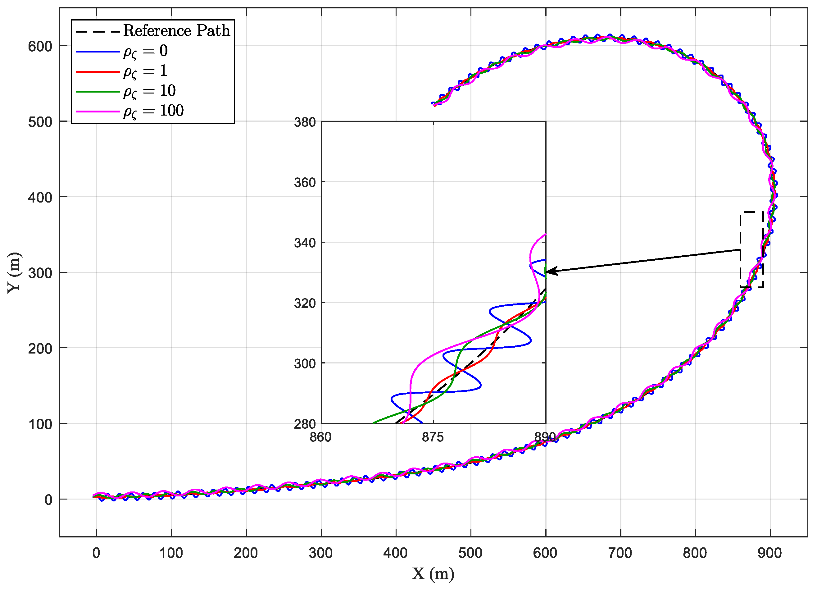
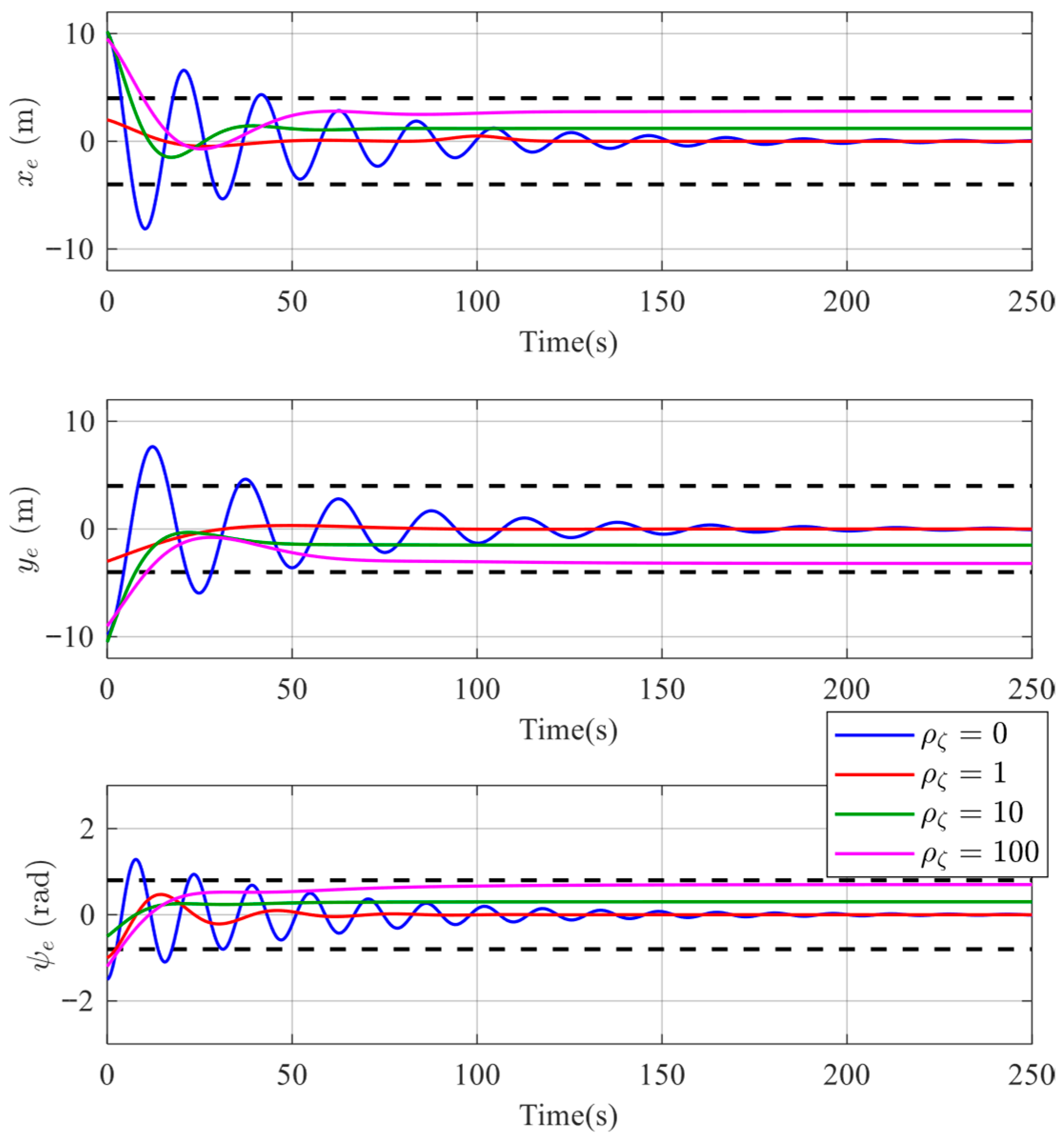
J k = i = 1 N p Y k + i k Y r e f k + i k Q 2 + i = 0 N c 1 Δ U k + i k R 2 + ρ ζ × ζ 2 ,
Therefore, the quadratic cost function adopted in (33) not only reflects the multi-objective control requirement of trajectory tracking, input smoothness, and constraint handling, but also provides a numerically tractable foundation for real-time optimization in the proposed RDO-MPC framework.
In this study, the control input of the RMPC is defined by the generalized surge thrust and yaw moment generated by the twin-thruster propulsion system of the USV. Therefore, the bounds U max and U min are determined from the actual actuator capability of this propulsion configuration rather than selected empirically. Specifically, the surge-force bounds are obtained from the maximum and minimum thrust that can be generated by the port and starboard thrusters, while the yaw-moment bounds are determined by the maximum differential moment achievable under the given thruster spacing and propulsion geometry. In addition, the input-rate bounds are introduced according to the allowable variation speed of the propulsion system to avoid excessive actuator wear and unrealizable command changes. The corresponding numerical values are summarized in Table 2 and are used as the baseline physical constraint set in the RMPC formulation. On this basis, when disturbance compensation is introduced, the admissible input region is further updated online through the dynamic constraint reconstruction mechanism so that the combined control input remains physically feasible.
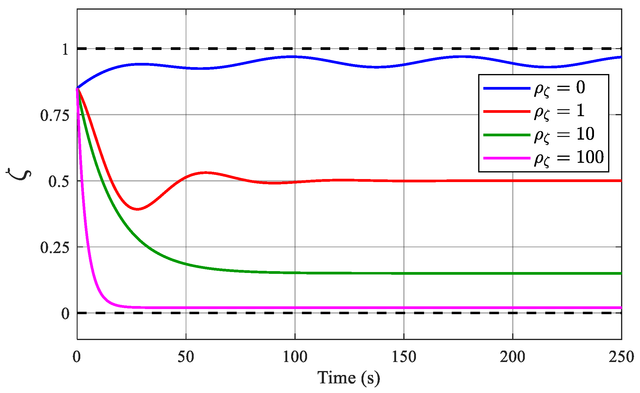
The main terms are interpreted as follows: Y r e f denotes the reference output, and Q is a positive definite weighting matrix that penalizes tracking errors in the longitudinal, lateral, and heading directions. Δ U represents the control input increments, while R is the corresponding weighting matrix, whose increase suppresses excessive control variations and protects actuators. The non-negative slack variable ζ , weighted by ρ ζ , is introduced to relax hard constraints into soft constraints, thereby avoiding infeasibility under extreme operating conditions and enhancing the numerical stability of the optimization problem.
The propulsion system of the USV is subject to explicit physical constraints, which must be taken into account in the optimization process:
(1)
Control input magnitude constraints, which limit the maximum thrust and rudder angle:
U min Δ U k + i k U max .
(2)
Control increment constraints, which limit the rudder rate and thrust rate:
Δ U min Δ U k + i k Δ U max .
(3)
Slack variable constraint, ensuring the non-negativity of the slack variable:
0 ζ 1 .
By integrating the constraints on control input magnitude, control increments, and the slack variable, they can be collectively formulated as the following linear inequality constraints:
Ω Δ U N c d c o n s + L ζ ,
where Ω denotes the constraint coefficient matrix, d c o n s represents the constraint boundary vector, and L is the coefficient vector corresponding to the slack variable.
Substituting the prediction equation into the cost function J k , and neglecting the constant terms that are independent of the optimization variables, the MPC optimization problem can be reformulated as a standard Quadratic Programming (QP) problem:
min Δ U N c , ζ 1 2 Δ U N c T H k Δ U N c + G k T Δ U N c + ρ ζ 2 s . t . Ω Δ U N c L ζ d c o n s 0 ζ 1 .
where H k and G k represent the Hessian matrix and the gradient vector, respectively.
The minimum of Equation (38) represents the optimal value of the finite-horizon cost function at the current sampling instant. Among all admissible control increment sequences satisfying the physical input limits, rate constraints, and soft-constraint conditions, the optimizer selects the sequence that yields the best trade-off between trajectory-tracking accuracy, control smoothness, and constraint satisfaction. Therefore, the minimization result is not only a numerical optimum, but also a quantitative measure of the best achievable predicted control performance over the current horizon. In the proposed RDO-MPC framework, it further reflects the optimal compromise between tracking quality and the reduced admissible control region induced by disturbance-compensation-aware constraint reconstruction. At each sampling instant k , the resulting QP problem is solved via an active-set or interior-point method, yielding the optimal control increment sequence Δ U N c .
Based on the receding horizon strategy of MPC, only the first element of the optimal control sequence is implemented at each time step. Thus, the MPC control input U m p c k is computed as follows:
U m p c k = U k 1 + Δ U k ,
The control input U m p c k is derived from the nominal disturbance-free model. Considering the existence of the lumped nonlinear disturbance d X , t introduced in the previous section, the use of U m p c k alone is insufficient to ensure high-accuracy trajectory tracking. Hence, U m p c k is treated as the nominal control component and is integrated with the output of the RBF-based adaptive sliding mode observer developed in the subsequent section, yielding the final composite robust control law.

3.2. Design of Adaptive Robust Disturbance Observer Based on RBFNN

Before presenting the observer equations, the rationale behind the disturbance approximation structure is clarified. The lumped disturbance term in (21) contains environmental loads, model uncertainty, and unmodeled nonlinear hydrodynamic effects, all of which are state dependent and difficult to parameterize explicitly. Since the RBF neural network possesses universal approximation capability for continuous nonlinear mappings over compact domains, it is employed to approximate the unknown disturbance as a function of the measurable system state. Based on this idea, the observer is constructed by combining three components:
(1)
A model-based nominal term describing the known system dynamics;
(2)
An adaptive RBFNN term estimating the state-dependent unknown disturbance online;
(3)
A robust sliding-mode correction term compensating for the neural approximation residual and guaranteeing bounded observation error.
With this structure, the observer can simultaneously exploit model information and maintain robustness against approximation errors.
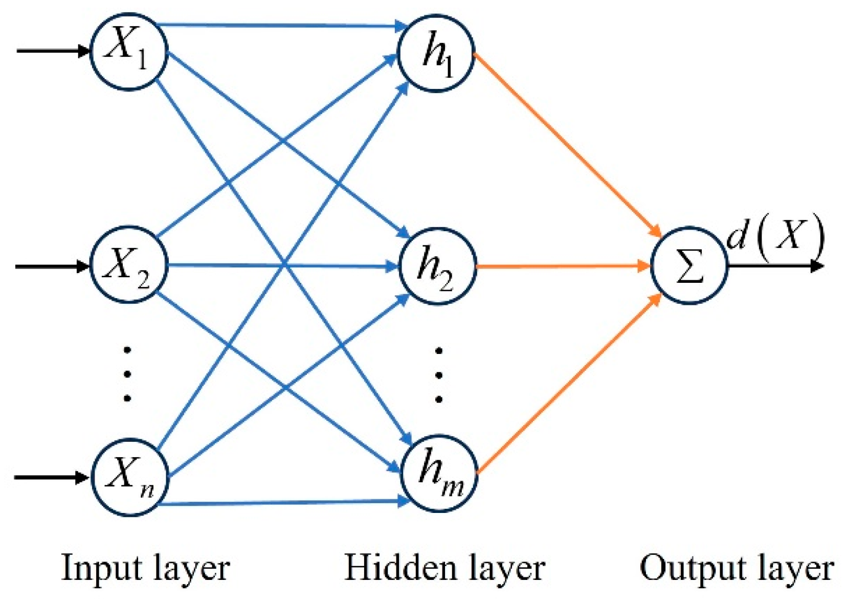
In the MPC design of the previous section, the system is approximated by a linear nominal model for receding-horizon optimization. Conventional adaptive control methods generally rely on linear parameterization of disturbances or estimate their constant bounds. However, real marine disturbances are inherently nonlinear and time-varying, rendering such approaches insufficient. Owing to its simple structure and strong universal approximation capability, the RBFNN can approximate any continuous nonlinear function with arbitrary accuracy [22]. Accordingly, an RBFNN-based adaptive robust disturbance observer is proposed. By combining a robust compensation term with the online learning capability of the RBFNN, the proposed method reconstructs unknown lumped disturbances and compensates for approximation errors, enabling accurate estimation and rejection of complex disturbances. The RBFNN architecture, as shown in Figure 3, consists of an input layer, a hidden layer, and an output layer.
To guarantee the mathematical rigor of the subsequent stability proof, the following assumptions are imposed to characterize the properties of the disturbance and the neural network:
Assumption 1. 
The lumped disturbance d X , t  acting on the system is a continuous function of the state  X , and is bounded over a compact set  d max > 0 , i.e., there exists a positive constant  ω max  such that d X , t ω max .
Assumption 2. 
For the RBF neural network, there exist an ideal weight matrix  W  and a bounded approximation error  ε X , such that for any  X Ω X , the disturbance  d X , t  can be approximated. Furthermore, there exists a sufficiently small positive constant  ε N , such that  ε X ε N  holds for all  X .
For the established nonlinear system X ˙ = f X + g X U + d X , t , the lumped disturbance d X , t is mainly composed of hydrodynamic parameter perturbations and environmental external forces. Its magnitude and direction are generally closely related to the current motion state of the USV. Assuming that the disturbance is a continuous function of the state X , it can be parameterized using the approximation capability of the RBF neural network. The input vector of the RBF neural network is defined as X i n . To accurately capture the state-dependent uncertainties in the system dynamics, the system state vector is selected as the network input, i.e., X i n = X . Accordingly, the disturbance function d X can be expressed as follows:
d X = W T h X i n + ε X i n = W T h X + ε X ,
The terms in the above expression are defined as follows: The vector h X denotes the Gaussian basis function vector, i.e., h X = h 1 X , , h m X T m , where m is the number of hidden layer nodes. The ideal weight matrix is denoted by W = arg min W m × n sup X Ω X ω ( X ) W T h ( X ) . The activation function of the j -th node is defined as follows:
h j X = exp X c j 2 2 b j 2 , j = 1 , 2 , , m .
where c j is the center vector of the j -th neuron, which is required to cover the state space of X , and b j denotes the width of the basis function.
In this section, considering the underactuated characteristics of the USV, separate observers are designed for the surge velocity u and yaw rate r channels. The system dynamics can be described as follows:
u ˙ = f u ( X ) + g u X τ u + d u ( X , t ) r ˙ = f r ( X ) + g r X τ r + d r ( X , t ) .
To achieve online reconstruction of the unknown nonlinear functions d u ( ) and d r ( ) , two independent RBF neural networks are constructed. By exploiting the approximation capability of the RBF neural network, an adaptive estimation layer for the disturbances is established [23]. For the surge and yaw channels, the disturbances can be expressed as follows:
d i ( X ) = W i T h ( X ) + ε i , i { u , r }   .
In the actual control process, the online estimates of the disturbances are computed using the estimated weights W ^ u and W ^ r as follows:
d ^ u = W ^ u T h ( X ) , d ^ r = W ^ r T h ( X ) .
To eliminate the neural network approximation residual ε i and enforce the convergence of the observation error, a state observer incorporating an adaptive sliding mode feedback term is designed.
Adaptive sliding mode observer for the surge channel:
u ^ ˙ = f u ( X ) + g X τ u + W ^ u T h ( X ) + k s 1 tanh ( β 1 u ˜ ) + k u u ˜ ,
W ^ ˙ u = Γ u u ˜ h ( X ) σ u W ^ u   .
where u ^ is the estimated state value; u ˜ = u u ^ is defined as the state observation error; k u > 0 is the linear feedback gain used to accelerate the convergence of the observation error; k s 1 > 0 is the robust sliding mode gain introduced to compensate for the neural network approximation residual ε u ; Γ u is a positive definite diagonal learning-rate matrix that determines the update speed of the weights; u ˜ h ( X ) is the main gradient-descent term, which drives the weights to evolve in the direction of reducing the observation error; and σ u > 0 is the modification coefficient. The purpose of introducing this damping term is to enhance the robustness of the algorithm in the presence of nonzero approximation errors, prevent parameter drift, and ensure that the weights remain bounded. The hyperbolic tangent function tanh ( β ) is adopted to replace the original sign function sgn ( ) , where β 1 > 0 is a tuning factor. This improvement preserves the robustness of sliding mode control while effectively eliminating the high-frequency chattering inherent in conventional sliding mode methods by smoothing the control action within the boundary layer. W ^ u denotes the estimated weights of the RBF neural network, and (45) gives the adaptive update law of the neural network weights. The detailed derivation will be presented in the stability analysis.
Adaptive sliding mode observer for the yaw channel:
r ^ ˙ = f r ( X ) + g X τ r + d ^ r + k s 2 tanh ( β 2 r ˜ ) + k r r ˜   ,
W ^ ˙ r = Γ r r ˜ h ( X ) σ r W ^ r   .
where r ^ is the estimated state value; r ˜ = r r ^ is defined as the state observation error; k r > 0 is the linear feedback gain used to accelerate the convergence of the observation error; k s 2 > 0 is the robust sliding mode gain introduced to compensate for the neural network approximation residual ε r ; Γ r is a positive definite diagonal learning-rate matrix that determines the update speed of the weights; r ˜ h ( X ) is the main gradient-descent term, which drives the weights to evolve in the direction of reducing the observation error; σ r > 0 . β 2 > 0 is the tuning factor. W ^ r denotes the estimated weights of the RBF neural network, and (47) gives the adaptive update law of the neural network weights. The detailed derivation will be presented in the stability analysis.
Based on the above analysis, the observation error dynamics can be derived as follows:
u ˜ ˙ = W ˜ u T h ( X ) + ε u k s 1 tanh ( β 1 u ˜ ) k u u ˜ r ˜ ˙ = W ˜ r T h ( X ) + ε r k s 2 tanh ( β 2 r ˜ ) k r r ˜ ,
where W ˜ u = W u W ^ u and W ˜ r = W r W ^ r denote the weight estimation errors.
Stability Analysis:
To rigorously establish the stability of the closed-loop system of the proposed observer, as well as the convergence of the RBF neural network weights, a detailed analysis is carried out based on Lyapunov stability theory.
Theorem 1. 
For the USV system subject to nonlinear disturbances, under the proposed observer structure and adaptive weight update laws, the observation errors  u ˜ , r ˜  , and the weight estimation errors  W ˜ u , W ˜ r , are uniformly ultimately bounded (UUB) in the closed-loop system.
Proof. 
Choose the Lyapunov candidate function V as the sum of the energy functions of the surge and yaw channels:
V = V u + V r = 1 2 u ˜ 2 + 1 2 t r W ˜ u T Γ u 1 W ˜ u + 1 2 r ˜ 2 + 1 2 t r W ˜ r T Γ r 1 W ˜ r ,
where t r denotes the trace of a matrix. Since Γ is a positive definite diagonal matrix, V t is positive definite.
Owing to the structural symmetry of the surge and yaw channels, the surge component V u is considered for the derivation. By differentiating V u with respect to time t , substituting the observation error dynamics and the adaptive update law, and noting that the ideal weight matrix W varies sufficiently slowly, together with W ˜ ˙ = W ^ ˙ , one obtains:
V ˙ u = u ˜ u ˜ ˙ W ˜ u T Γ u 1 W ^ ˙ u = u ˜ W ˜ u T h ( X ) + ε u k s 1 tanh ( β 1 u ˜ ) k u u ˜ W ˜ u T u ˜ h ( X ) σ u W ^ u , = k u u ˜ 2 + u ˜ ε u k s 1 u ˜ tanh ( β 1 u ˜ ) + σ u W ˜ u T W ^ u
Considering W ^ u = W u W ˜ u , the last term σ u W ˜ u T W ^ u is scaled using the inequality a T ( b a ) 1 / 2 b 2 a 2 :
σ u W ˜ u T ( W u W ˜ u ) σ u 2 W u 2 σ u 2 W ˜ u 2   .
For the robust compensation term, when β 1 is sufficiently large, u ˜ tanh ( β 1 u ˜ ) | u ˜ | . By selecting the robust compensation gain to satisfy k s 1 ε ¯ u , it follows that u ˜ ε u k s 1 u ˜ tanh ( β 1 u ˜ ) 0 .
To simplify the analysis, a general bounding form is retained, and Young’s inequality is applied to the term x y 1 / 2 x 2 + y 2 :
u ˜ ε u 1 2 u ˜ 2 + 1 2 ε ¯ u 2 .
By combining the above results, the following expression can be derived:
V ˙ u ( k u 1 2 ) u ˜ 2 σ u 2 W u 2 + 1 2 ε ¯ u 2 + σ u 2 W u 2   .
By appropriately selecting the linear gain k u > 0.5 , and defining the constants χ u = min ( 2 ( k u 0.5 ) , σ u λ min ( Γ u ) ) and ϑ u = 1 / 2 ε ¯ u 2 + σ u W u 2 , it follows that:
V ˙ u χ u V u + ϑ u .
The stability analysis for the yaw channel follows in a similar manner. By combining the results of the surge and yaw channels, the total time derivative of the Lyapunov function satisfies:
V ˙ = V ˙ u + V ˙ r χ u V u + ϑ u χ r V r + ϑ r min ( χ u , ϑ r ) ( χ u + ϑ r ) + ( χ u + ϑ r ) .
By defining χ = min ( χ u , χ r ) > 0 and ϑ = ϑ u + ϑ r > 0 , it follows that:
V ˙ χ V + ϑ .
Conclusions: The above stability analysis constitutes a complete proof of Theorem 1. From the above inequality, it can be seen that when the system energy satisfies V > ϑ / χ , the time derivative of V ˙ becomes strictly negative. This implies that the system state trajectories will converge to and remain within a compact set Ω V = { ( u ˜ , r ˜ , W ˜ ) | V ϑ / χ } centered at the origin. Therefore, the proposed RBF-based adaptive disturbance observer guarantees the uniform ultimate boundedness of both the observation errors and the weight estimation errors. Moreover, the disturbance estimate d ^ u , d ^ r can effectively approximate the actual disturbance, thereby providing a reliable feedforward signal for the subsequent composite control design.

3.3. Synthesis of Composite Control Laws

In conventional composite control strategies, disturbance compensation is typically designed as an independent feedforward term and directly superimposed onto the feedback control law. However, the propellers and rudders of a USV are subject to strict physical constraints on both magnitude and rate of change. If the coupling between these two is neglected, the control input generated by disturbance compensation may occupy excessive actuator capacity, causing the optimal control input computed by the MPC controller to exceed the physical limits after superposition. This may not only lead to control interruption and degrade the optimization performance of MPC, but in severe cases, may even result in instability of the closed-loop system.
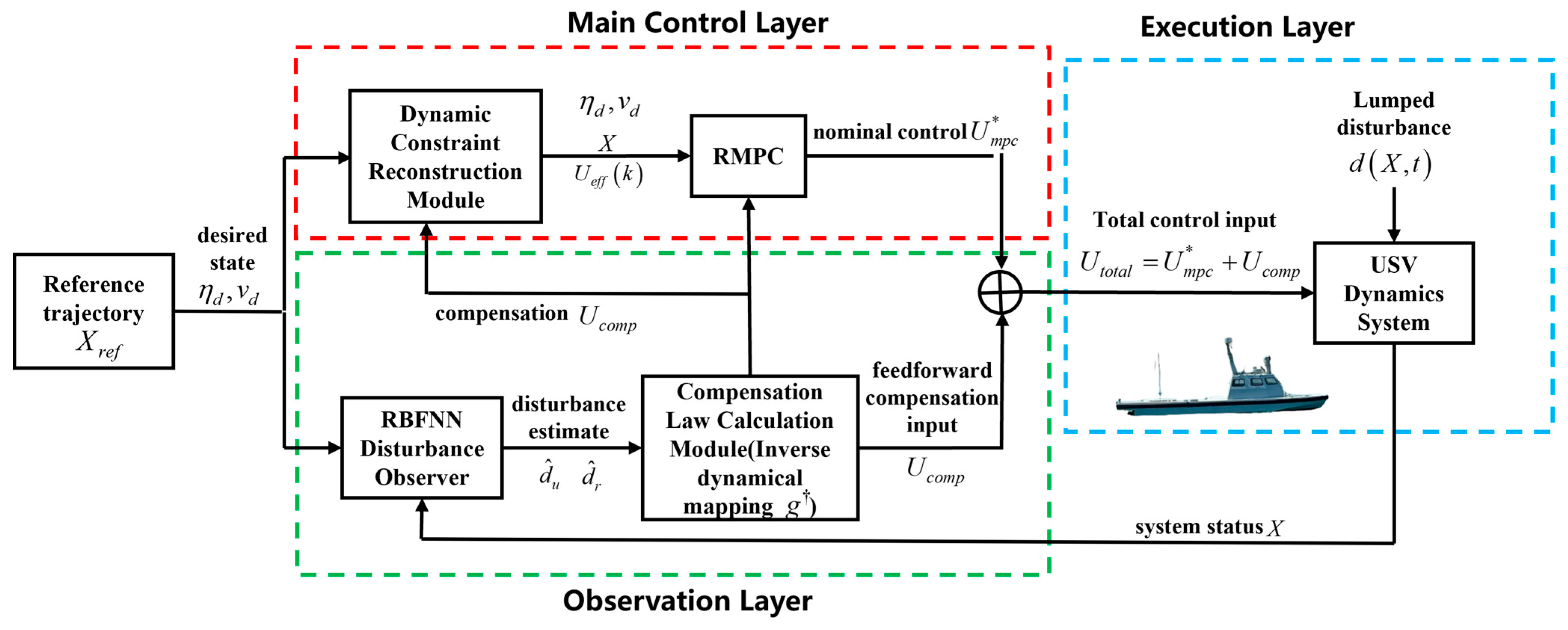
To address the aforementioned issues, this section proposes an RBF neural network observer-based robust disturbance optimization MPC (RDO-MPC) scheme, as illustrated in Figure 4. The proposed strategy employs an RBF-based adaptive robust disturbance observer to perform feedforward disturbance compensation. Meanwhile, the corresponding compensation demand is fed back to the MPC controller in real time to dynamically reconstruct the constraint boundaries of the optimization problem, thereby ensuring the physical feasibility of the overall control input.
The system consists of two core information flow channels, each responsible for different control tasks. The disturbance suppression channel is dominated by the designed disturbance observer. Specifically, the observer reconstructs the lumped disturbances d u X , t and d r X , t online, yielding their estimates d ^ u , d ^ r . Based on the inverse dynamics model of the USV, an equivalent compensation control input U c o m p is then computed to counteract the disturbances. This signal is directly injected into the low-level actuation system, with the objective of transforming the disturbed nonlinear system into a nominal linear system. The constraint optimization channel flows from the compensation module to the MPC controller. The estimated compensation input U c o m p is fed back to the MPC as prior information. Based on this information, the MPC dynamically shrinks its admissible control constraint set in real time. This implies that, during the receding-horizon optimization process, the MPC has already reserved sufficient control authority for disturbance rejection, thereby ensuring that the sum of the optimal control input U m p c k and the compensation input U c o m p strictly satisfies the physical constraints.
Based on the established affine nonlinear dynamic model of the USV, in order to eliminate the influence of the disturbance term d X , t on the system dynamics, an ideal feedforward compensation control law U c o m p = τ c o m p , u , 0 , τ c o m p , r T is defined. The ideal compensation input U c o m p should satisfy the following matching condition:
g X U c o m p + d X , t = 0 .
The real disturbance is replaced by its online estimate d ^ X = W ^ T h X . Considering that the USV model is underactuated, the input matrix g X is non-square and therefore cannot be directly inverted. To map the disturbance estimate vector d ^ into the control input space, the left pseudo-inverse in the least-squares sense is adopted for inverse dynamics mapping. The pseudo-inverse matrix of g X , denoted by g ( X ) , and its corresponding formulation are given as follows:
g ( X ) = g T ( X ) g ( X ) 1 g T ( X ) .
The disturbance compensation control law is then obtained as follows:
U c o m p ( k ) = g ( X k ) d ^ ( k ) .
The above control law can only compensate for matched disturbances, whereas unmatched disturbances may still persist in the system. To avoid violation of actuator limits by the total control input U t o t a l = U m p c + U c o m p , the constraints of the MPC optimization problem must be dynamically adjusted. Let the physical hard constraint set of the USV actuators be defined as U max :
U max = { U 2 U l i m U U l i m }   .
Specifically, for the surge thrust and yaw moment, the constraints are imposed as | τ u | τ u , lim and | τ r | τ r , lim .
At time instant k , the effective control constraint set available to the MPC controller, denoted by U e f f k , is defined as the physical constraint set minus the compensation input at the current time step:
U e f f k = U 2 U + U c o m p k U max .
Specifically, the amplitude constraint boundaries in the MPC optimization problem are reconstructed according to the following rule:
τ u , max e f f ( k ) = τ u , lim | τ c o m p , u ( k ) | U s a f e τ r , max e f f ( k ) = τ r , lim | τ c o m p , r ( k ) | U s a f e ,
where U s a f e is a safety threshold introduced to prevent numerical errors.
In the dynamic constraint reconstruction mechanism, the effective constraint bounds τ u , max e f f and τ r , max e f f defined above may shrink significantly as the disturbance compensation input U c o m p increases. Under extreme sea conditions, excessively large disturbances may cause the feasible set under hard constraints to become empty, leading to failure of the MPC optimization. This is precisely the main motivation for introducing the slack variable ζ and its associated constraints in the MPC cost function.
By introducing ζ , the original hard constraints are transformed into soft constraints. Accordingly, the constraint inequality in the quadratic programming (QP) problem, originally expressed as Ω Δ U N c d c o n s + L ζ , is reformulated into a dynamic form. When the physical constraint set is severely compressed or even infeasible, the solver can increase ζ to recover feasibility. Due to the inclusion of the penalty term ρ ζ ζ 2 with a large weight ρ ζ , the optimizer prioritizes constraint satisfaction and only relaxes constraints when unavoidable, with minimal cost. This guarantees QP feasibility and ensures safe and continuous operation of the USV system.
By integrating the above design components, the overall control input U t o t a l k applied to the USV propulsion system is formulated as follows:
U t o t a l k = U m p c k + U c o m p k .
The closed-loop control procedure is described as follows:
Step 1: At the sampling instant k , the USV state X k is obtained. The RBFNN-based adaptive robust disturbance observer updates the network weights W ^ u , W ^ r according to the adaptive laws, based on the current state and the control input at the previous time step. It then outputs the estimated disturbances for the surge and yaw channels, denoted by d ^ u and d ^ r , respectively.
Step 2: The feedforward compensation control input U c o m p k is computed using the pseudo-inverse matrix. Based on the physical limits τ u , lim and τ r , lim , together with the current compensation input U c o m p k , the effective MPC constraint bounds τ max e f f are determined.
Step 3: The MPC receding-horizon optimization incorporates the updated effective constraint bounds τ max e f f into the formulated QP problem. The optimal nominal control increment Δ U k and the corresponding control input U m p c k are then obtained.
Step 4: The total control input U t o t a l k is computed. Since U m p c k is obtained under the constraint τ max e f f , it theoretically satisfies | U m p c + U c o m p | τ lim , thereby strictly ensuring the physical safety of the actuators.

3.4. Stability Analysis of Closed-Loop System

Theorem 1 rigorously proves, based on Lyapunov theory, that the RBFNN-based disturbance observer guarantees the uniform ultimate boundedness of the observation errors u ˜ , r ˜ , as well as the weight estimation errors d ^ u , d ^ r . However, the convergence of the observer is only a necessary but not sufficient condition for the stability of the closed-loop system. To further establish the trajectory tracking stability of the USV under the proposed RDO-MPC framework—comprising feedforward compensation via the adaptive robust disturbance observer and dynamic constraint reconstruction—this section introduces the Input-to-State Stability (ISS) theory to analyze the dynamic behavior of the closed-loop system [24].
Closed-loop error dynamics modeling based on the USV dynamic equation X ˙ , when the designed composite control law U t o t a l is substituted into the system [25]. Considering that the disturbance compensation law is designed as U c o m p , and under the matching condition assumption that g X g ( X ) I , the closed-loop system can be rewritten as follows:
X ˙ = f X + g X U m p c g X d ^ X , t + d X , t = f X + g X U m p c d ^ X , t + d X , t = f X + g X U m p c + d ˜ X , t .
where d ˜ X , t = d X , t d ^ X , t denotes the disturbance estimation residual, and d X , t = [ d u X , t , 0 , d r X , t ] T is the actual disturbance vector. From the above equation, it can be observed that the closed-loop system under the composite control scheme is mathematically equivalent to a standard nonlinear system driven by an external bounded input d ˜ .
Assumption 3. 
The external environmental disturbance is bounded within the physically attainable domain of the USV actuators, i.e.,  sup t g d ( X , t ) < U max . If this bound is exceeded, the system will enter the actuator saturation region, where stability can only be maintained by the slack variable and the inherent passive damping of the system.
Theorem 2. 
Suppose that the designed RMPC controller guarantees asymptotic stability of the nominal system in the disturbance-free case  d ˜ = 0 , and that the optimal value function  J X  of the RMPC satisfies the Lipschitz continuity condition. Meanwhile, the designed observer ensures that the disturbance estimation error is bounded. Then, under the proposed composite control law, the closed-loop system state  X t  is uniformly ultimately bounded (UUB), and the system exhibits input-to-state stability (ISS).
Remark 1. 
The introduction of the slack variable transforms the original hard constraints into soft constraints, thereby preventing optimizer failure in extreme operating conditions. However, soft-constraint feasibility should not be interpreted as equivalent to closed-loop stability. In this work, the slack variable is used only to preserve optimization feasibility, whereas the practical stability result is established through the terminal RMPC design and the boundedness of the observer-induced residual perturbation.
Remark 2. 
Since the effective input constraint set varies online with the disturbance compensation signal, the resulting optimization problem is time-varying. Therefore, the stability analysis does not directly invoke the standard unconstrained or fixed-constraint MPC result, but instead interprets the online constraint adaptation as a bounded time-varying perturbation to the nominal RMPC framework.
Proof. 
The optimal value function J X of the MPC optimization problem is selected as the Lyapunov candidate function V N ( ) for the closed-loop system. According to the stability theory of robust MPC [26], for a finite-horizon controller with terminal constraints or terminal penalties, the optimal value function satisfies the following properties:
Property 1: Positive definiteness and radial unboundedness. There exist class K functions α 1 ( ) , α 2 ( ) such that:
α 1 ( X k ) V N ( X k ) α 2 ( X k ) .
Property 2: Under the nominal control law U m p c , the time derivative of V N ( ) along the trajectories of the nominal system satisfies:
V N ( X ( k + 1 ) | X ( k ) , nominal ) V N ( X ( k ) ) α 3 ( X ( k ) )   .
Property 3: Lipschitz continuity. There exists a constant L v > 0 such that, for any state perturbation Δ X , it holds that:
| V N ( X + Δ X ) V N ( X ) | L v Δ X   .
For the disturbed system, the actual state X ( k + 1 ) at time instant k + 1 consists of the nominal predicted state and a deviation term Δ X d ( k ) induced by the disturbance estimation residual. According to the discrete-time model, this deviation satisfies Δ X d ( k ) T s d ˜ ( k ) , where T s is the sampling time.
The difference in the Lyapunov function for the actual closed-loop system is calculated as follows:
Δ V = V N ( X ( k + 1 ) ) V N ( X ( k ) ) = V N ( X n o m ( k + 1 ) + Δ X d ( k ) ) V N ( X ( k ) ) .
Using the Lipschitz continuity condition together with the triangle inequality, the above expression can be further expanded as follows:
Δ V V N ( X n o m ( k + 1 ) ) V N ( X ( k ) ) + L v Δ X d ( k ) α 3 ( X ( k ) ) + L v T s d ˜ ( k ) ,
From inequality (70), it can be observed that the convergence behavior of the system depends on the magnitude of the current state error X ( k ) . When the state error is sufficiently large such that α 3 ( X ( k ) ) > L v T s Δ d , it follows that Δ V < 0 . This implies that the Lyapunov function decreases monotonically, driving the system state trajectories toward the origin. Therefore, the closed-loop system state X ( t ) will ultimately converge to and remain within a compact set Ω X = { X α 3 ( X ) L v T s Δ d } in the neighborhood of the origin. □
Conclusions: Since Δ d depends on the approximation error of the RBFNN and the chattering effect of the sliding mode observer, it can theoretically be made arbitrarily small by increasing the number of neural network nodes and appropriately tuning the parameters of the robust compensation term. Therefore, the compact set Ω X can be made an arbitrarily small neighborhood around the origin. This demonstrates that the closed-loop system under the proposed composite control law is input-to-state stable (ISS) and capable of achieving high-precision trajectory tracking. Even under strict physical constraints and strong disturbances, the system does not exhibit divergence or instability.
The above analysis completes the proof of Theorem 2. From a theoretical perspective, the effectiveness and stability of the proposed RDO-MPC control scheme are verified. In the next subsection, numerical simulations of the closed-loop system and the control algorithm will be conducted to further validate the feasibility of the proposed method.

4. Numerical Simulation

4.1. Simulation Experiment Setup

To comprehensively evaluate the trajectory tracking performance and robustness of the proposed RDO-MPC control strategy under complex marine environments, this section first establishes the fundamental framework of the simulation experiments. The experimental setup mainly consists of three components: dynamic generation of reference trajectories, specification of the physical constraints of the controlled system, and tuning of key controller parameters.
The simulation object is a large-scale underactuated USV with a displacement of 9800 kg, whose detailed dynamic model parameters are provided in Table 1. To evaluate the effectiveness of the proposed algorithm under physical limits, strict magnitude and rate constraints are imposed on the actuators. The USV propulsion system consists of a main propeller and a rudder, and the corresponding physical constraint parameters are listed in Table 2.
The selection of controller parameters is directly related to the tracking accuracy and stability of the system. The specific parameters of the proposed RDO-MPC trajectory tracking controller for the USV are given as follows: k u = 5 , k r = 5 , k s 1 = 0.01 , k s 2 = 0.01 , β 1 = 0.1 , β 2 = 0.1 , ζ = 0.5 , Γ r = d i a g 0.2 , 0.2 , 0.2 , Γ u = d i a g 0.5 , 0.5 , 0.5 , σ u = 1 × 10 4 , σ r = 2.5 × 10 5 . In the simulation experiments, RBF neural network models are employed to approximate the unknown nonlinear dynamics of the USV and the environmental disturbances. Two RBF networks are used in total. The inputs of each network are the surge velocity u , sway velocity v , and yaw rate r of the USV. The number of hidden layer nodes is m = 9 , and the center vectors c j are [ 5 , 5 ] × [ 5 , 5 ] . The widths of the Gaussian basis functions are set as b 1 = 1.5 , b 2 = 1 , respectively. The remaining key parameters are listed in Table 3.
The RMPC parameters listed in Table 3 are determined according to the dynamic characteristics of the considered USV platform and the control objective of constrained-water trajectory tracking. Since the studied platform is a 9800 kg large-scale underactuated USV, its maneuvering process exhibits relatively large inertia. In this case, insufficient emphasis on the tracking states may lead to slow correction of maneuvering deviation. Moreover, because the sway motion is not directly actuated, the lateral tracking error is mainly reduced through heading adjustment and surge-motion coordination. Therefore, the state-error weighting matrix is chosen as Q = diag 10 3 , 10 3 , 5 × 10 3 , in which the heading-related term is assigned a larger weight to suppress the accumulation of lateral-position error caused by persistent heading mismatch, especially in the time-varying curvature and large-maneuver scenarios.
The control-increment weighting matrix is selected as R = diag [ 0.1 , 0.1 , 0.1 ] . The relatively small values are used to maintain sufficient correction capability for the large-mass platform, while the smoothness of the control input is still constrained by the increment penalty and the explicit actuator magnitude/rate limits. In addition, the prediction horizon N p = 30 and control horizon N c = 5 are chosen by balancing trajectory prediction capability and online computational feasibility. The final parameter set is obtained through repeated simulation-based tuning under the representative scenarios considered in this paper.
For a fair and reproducible comparison, the benchmark controllers in Section 4 are configured under the same USV model, reference trajectories, simulation duration, sampling conditions, parameter-variation settings, and actuator magnitude/rate constraints as the proposed method. Specifically, the reference MPC employs the same prediction model and predictive-control structure as the nominal optimization layer of the proposed framework, but does not include the disturbance observer, feedforward compensation, or dynamic constraint reconstruction. The benchmark ASMC is implemented on the same 3-DOF tracking-error model and evaluated under the same operating scenarios to represent a disturbance-rejection-oriented feedback controller without predictive optimization.
In addition to the reference-trajectory design and controller parameter settings, the simulation model also considers the influence of realistic marine environmental disturbances. As described in Equations (12)–(16), the external disturbance acting on the USV is represented by a lumped disturbance term that combines current, wind, and wave effects together with parameter perturbation and unmodeled nonlinear dynamics. This formulation is adopted to reflect the coupled uncertainty characteristics commonly encountered in constrained waters, rather than an idealized single-source disturbance condition.
To evaluate the proposed controller under progressively more demanding operating conditions, three representative simulation scenarios are designed. All scenarios are conducted under the above lumped disturbance setting, while their main difference lies in the complexity of the reference trajectory and the degree of uncertainty emphasized in each test. In this way, the simulation study not only examines tracking performance under regular path evolution, but also evaluates controller robustness and compensation effectiveness under stronger maneuvering nonlinearity and parameter variation. The initial state of the USV is set as X ( 0 ) = [ 5 , 2 , 0 , 0 , 0 , 0 ] T .
(1)
Scenario 1: The desired trajectory is a sinusoidal curve, which is commonly used to evaluate controller performance.
(2)
Scenario 2: The curvature of the desired reference trajectory varies over time. Compared with Scenario 1, this scenario imposes more stringent conditions and increases the difficulty of trajectory tracking.
(3)
Scenario 3: The curvature of the desired reference trajectory varies over time. By comparing the tracking performance under different controller parameter settings, this scenario is used to evaluate the effect of the RBF neural network-based online compensation on the RMPC trajectory tracking performance.

4.2. Simulation Results and Analysis

To comprehensively evaluate the proposed RDO-MPC strategy without relying on a single trajectory-tracking metric, the simulation study is organized into three complementary tests. Test 1 focuses on the basic tracking capability and robustness under nominal and parameter-perturbed sinusoidal trajectories. Test 2 further examines the dynamic response and tracking performance under continuously varying curvature, which imposes stronger nonlinear maneuvering demands. Test 3 is designed to investigate the effectiveness of the disturbance-observer-based compensation mechanism under large-maneuver conditions with accumulated model uncertainty, with particular attention to state-estimation accuracy, compensation behavior, and actuator-feasible control. In addition to the trajectory and error plots, a cumulative performance index based on Equation (33) is introduced to provide a quantitative comparison of the overall optimization performance.
(1)
Test 1: Sinusoidal trajectory tracking. Under the first path condition, the reference trajectory generated by the virtual vessel is defined by the following mathematical expression:
x d ( t ) = 1.0 t y d ( t ) = 20 sin ( 0.04 t ) .
The corresponding desired surge velocity is approximately 5 m/s, accompanied by periodic heading adjustments. The simulation duration is set to 200 s. The controller proposed in this chapter is denoted as RDO-MPC, and for comparison, MPC and ASMC controllers are simulated for the same reference trajectory.
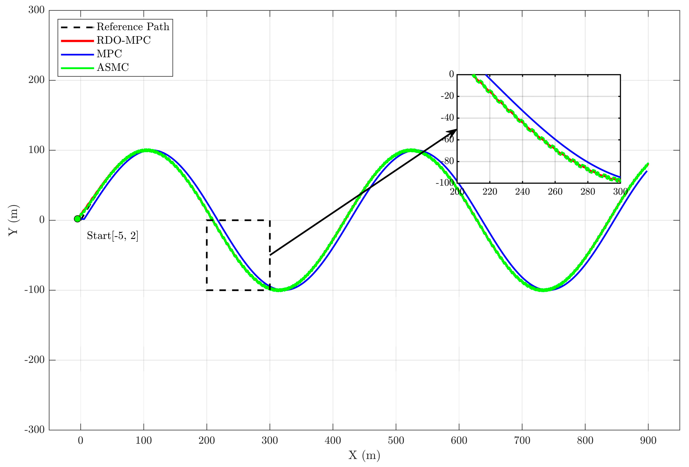
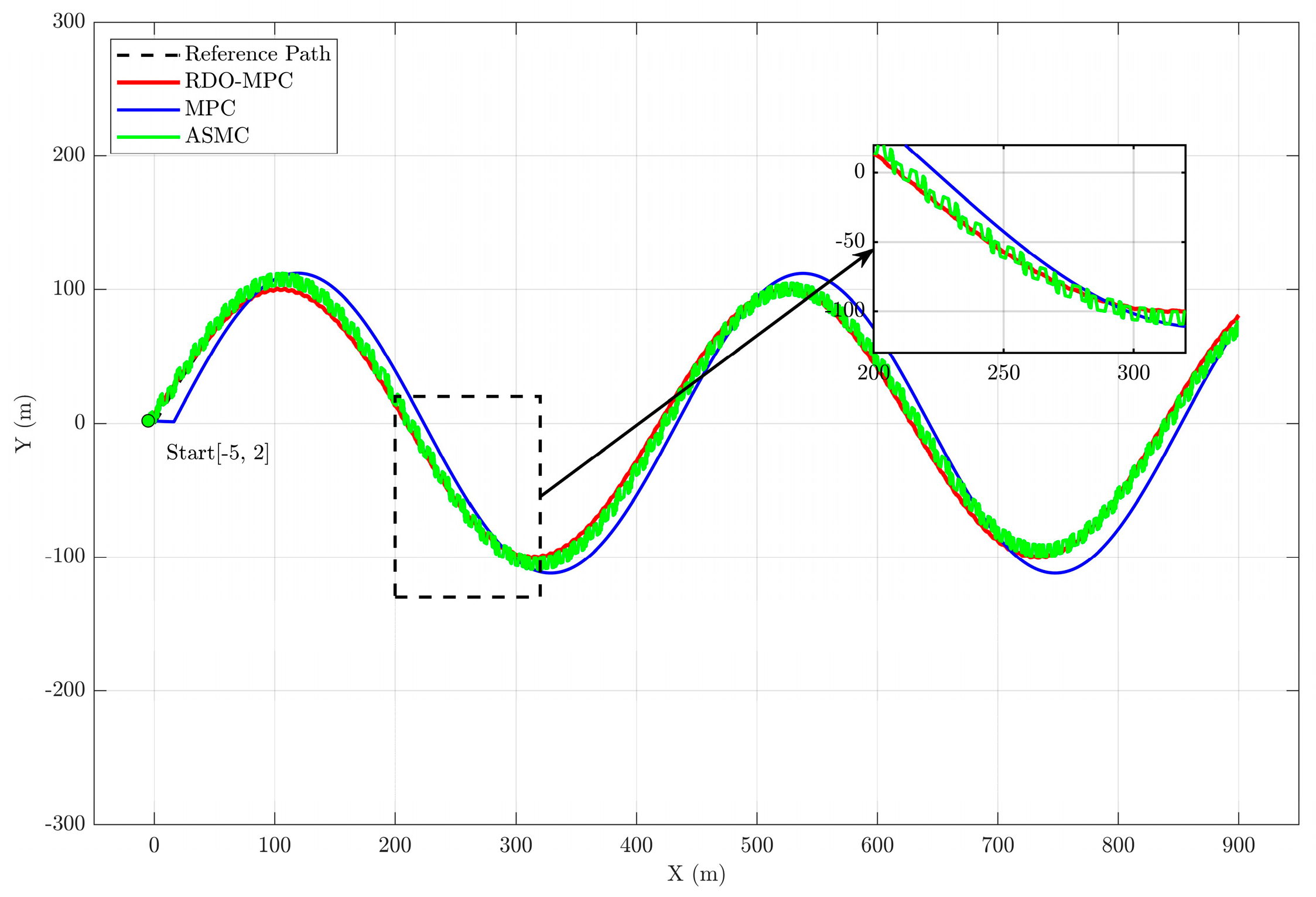
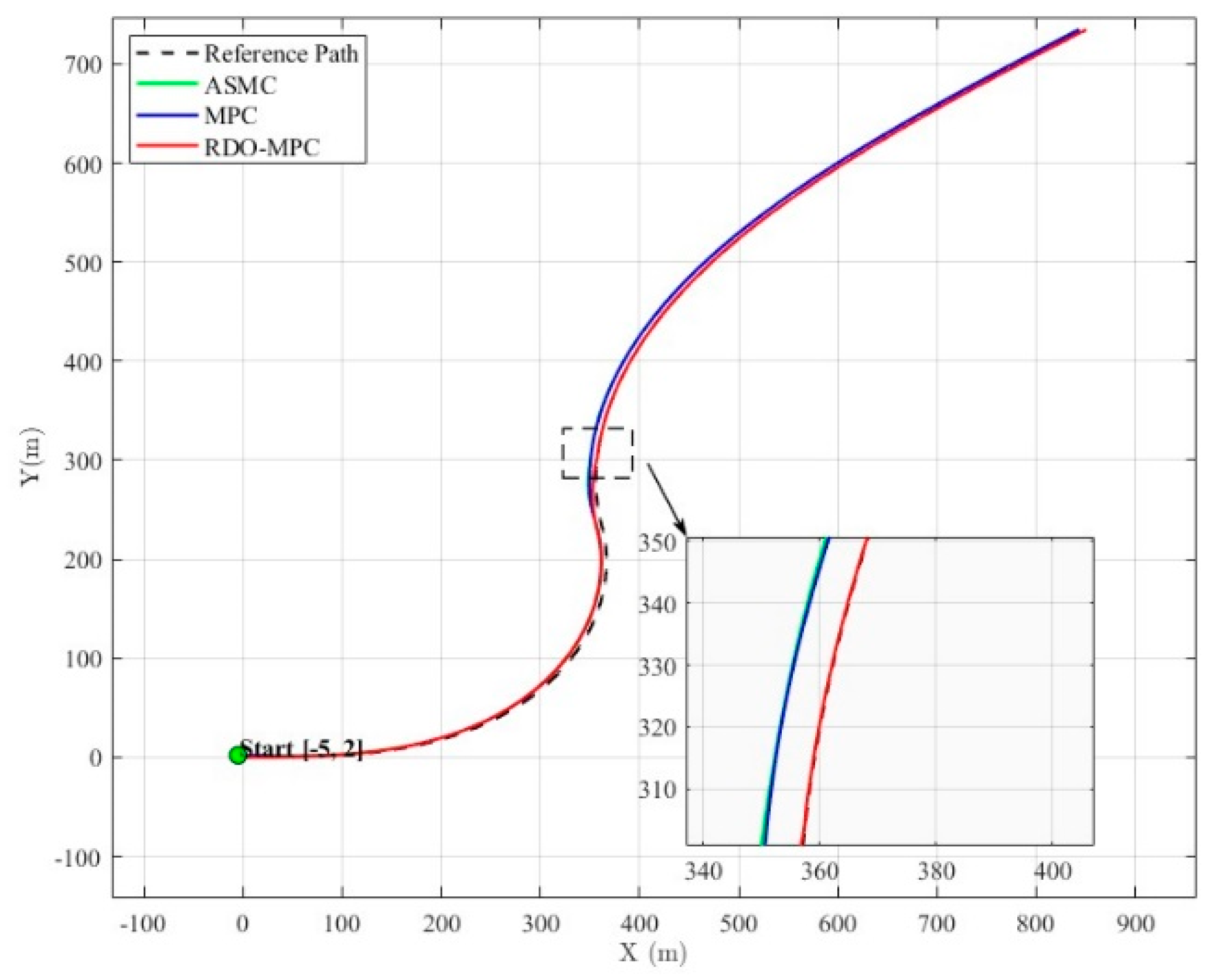
Figure 5 and Figure 6 illustrate the trajectory tracking performance of the three control algorithms. Figure 5 shows the tracking results of the USV without model parameter disturbances, while Figure 6 presents the results when a 10% perturbation is introduced into the model parameters used for controller design.
From the enlarged view of Figure 5, it can be observed that the proposed RDO-MPC algorithm achieves smaller steady-state tracking errors compared to the other two methods. Furthermore, as shown in Figure 6, under parameter perturbations, the proposed method demonstrates strong robustness against model uncertainties and environmental disturbances, with the lateral tracking error reduced by 4.63 m and 1.01 m, respectively.
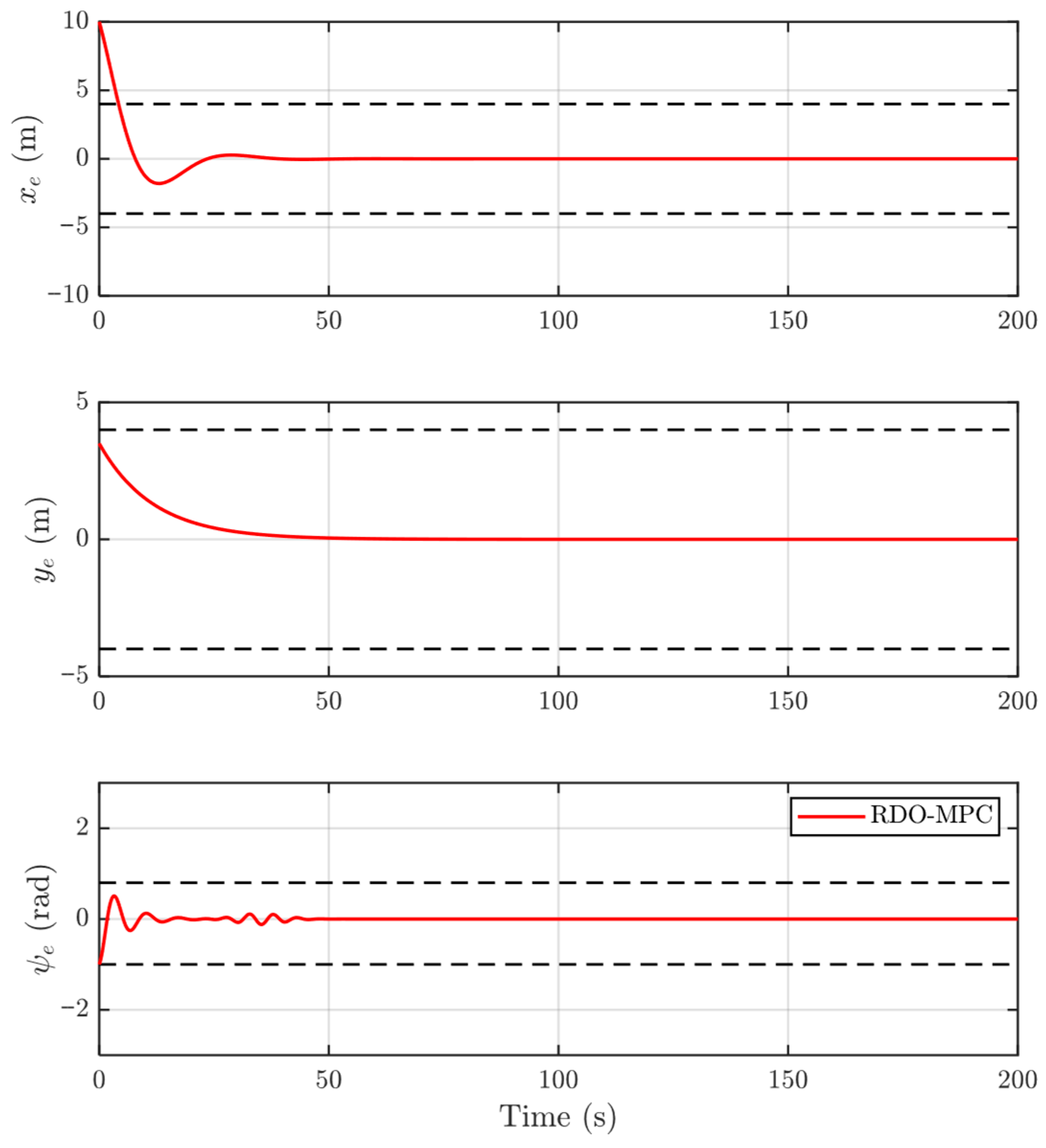
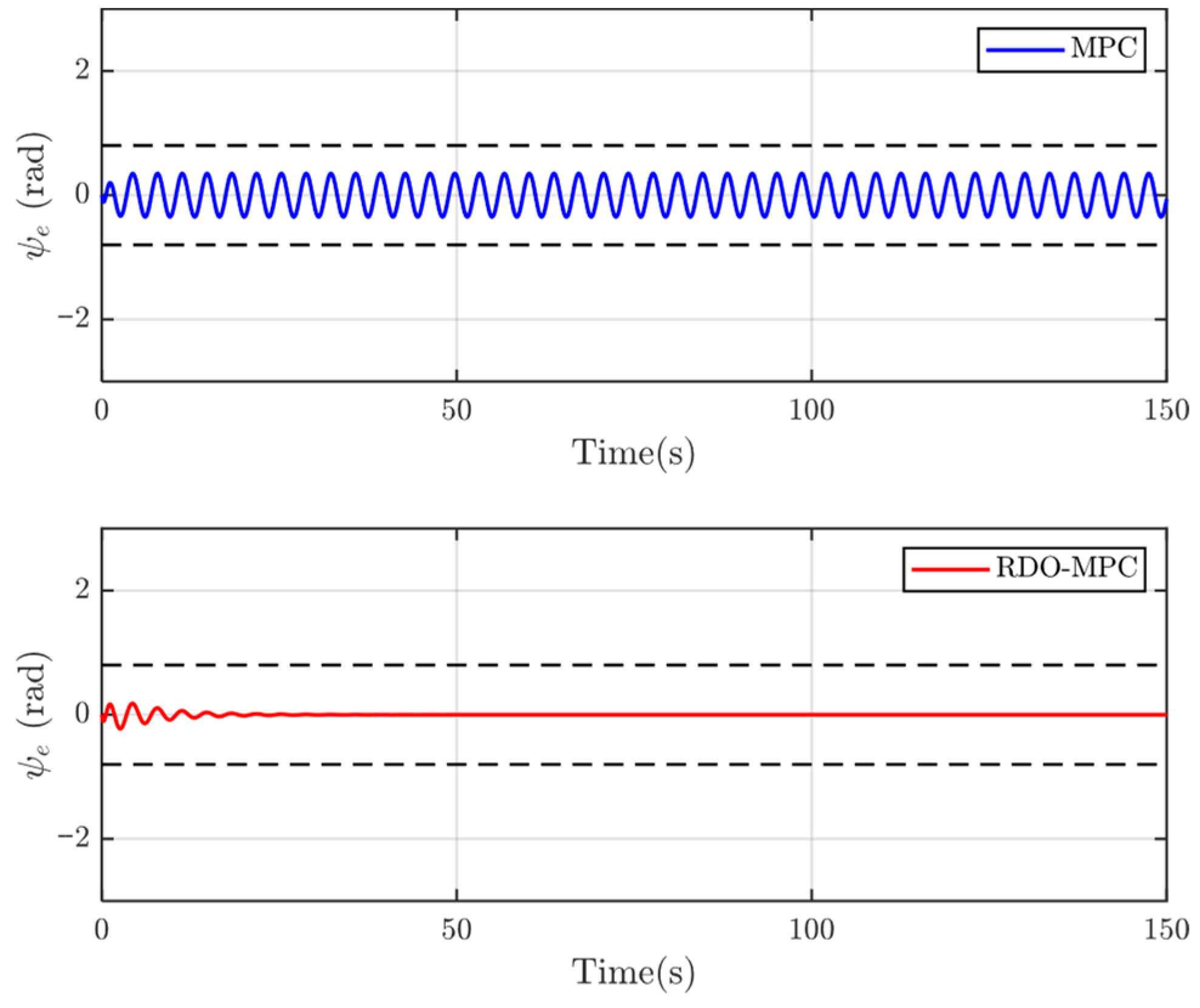
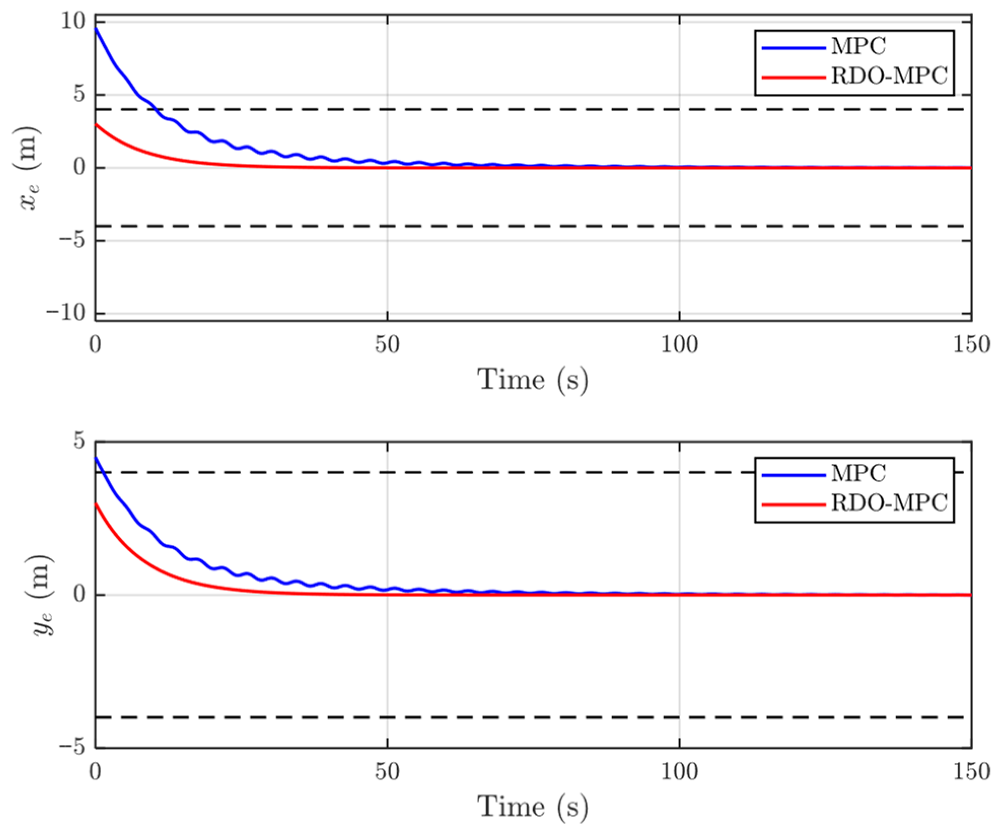
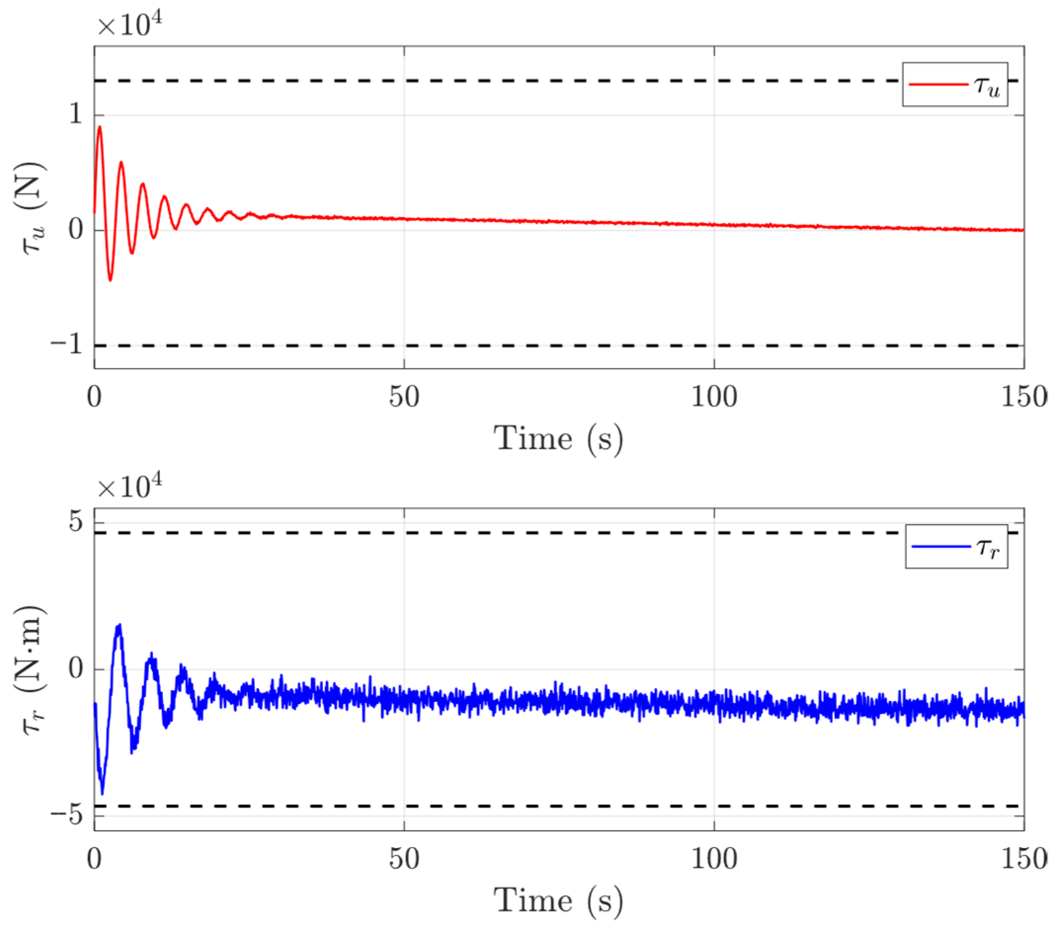
Figure 7 presents the evolution of the constrained state error variables when trajectory tracking is performed using the proposed RDO-MPC algorithm under the nominal condition without parameter perturbations. By incorporating the RBF neural network observer and sliding mode control, model uncertainties are effectively compensated.
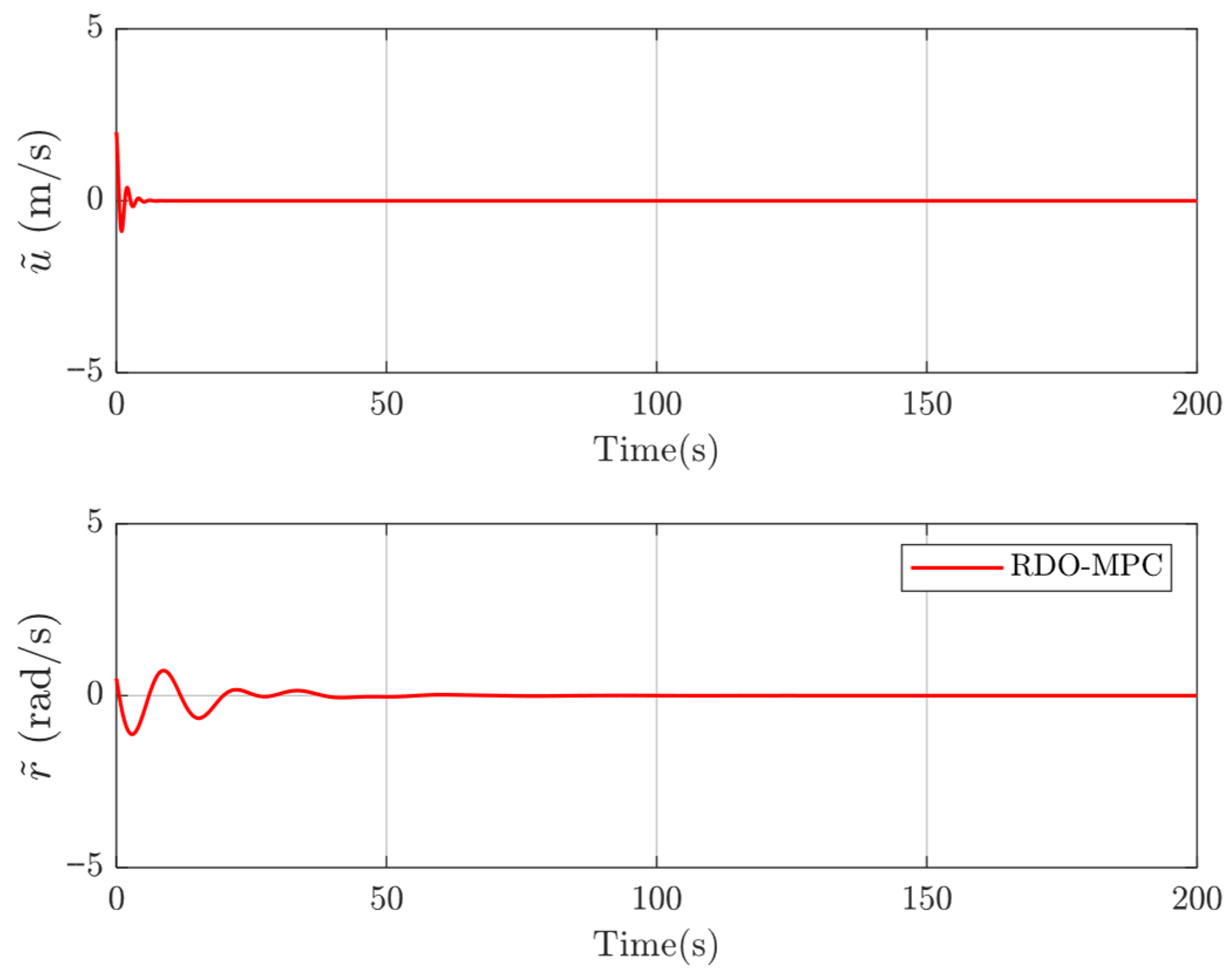
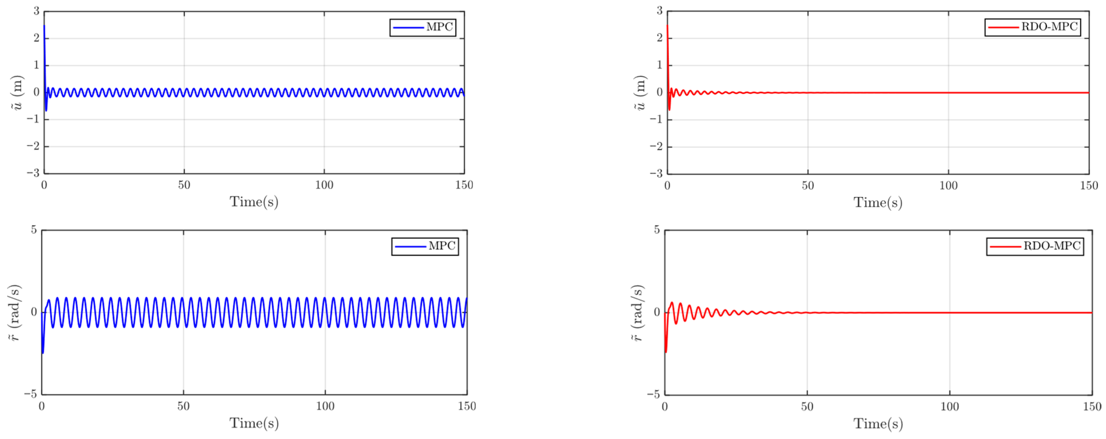
Figure 8 illustrates the state observation errors of u ˜ and r ˜ in the controller design. As observed from the figures, the design based on Lyapunov stability theory ensures the convergence and stability of the intermediate variables, and both observation errors ultimately converge to a neighborhood around zero.
Based on the results shown in Figure 5, Figure 6, Figure 7 and Figure 8, it can be concluded that the proposed RDO-MPC algorithm exhibits excellent control performance, strong disturbance rejection capability, and robust system behavior when tracking the sinusoidal trajectory.
(2)
Test 2: To further evaluate the robustness of the controller under more challenging conditions, Scenario 2 considers a complex trajectory with continuously and rapidly varying curvature over time. Compared with Scenario 1, this scenario not only introduces a nonlinear variation in the reference angular velocity, but also significantly amplifies the hydrodynamic nonlinear effects acting on the USV. Moreover, abrupt changes in angular velocity may induce large lateral deviations, posing higher requirements on the dynamic response capability and prediction accuracy of the controller. In this test, the reference trajectory generated by the virtual guidance vessel is described as follows:
u d = 5   m / s r d = { 0.1 e 0.004 t 0.1 r a d / s , 0 t < 100 0.03 tanh ( 0.01 ( t 100 ) ) 0.03 r a d / s , t 100 .
The total simulation time is set to 250 s. The controller parameters remain the same as those in Scenario 1. The tracking path is a trajectory with continuously varying curvature, while all other conditions remain unchanged.
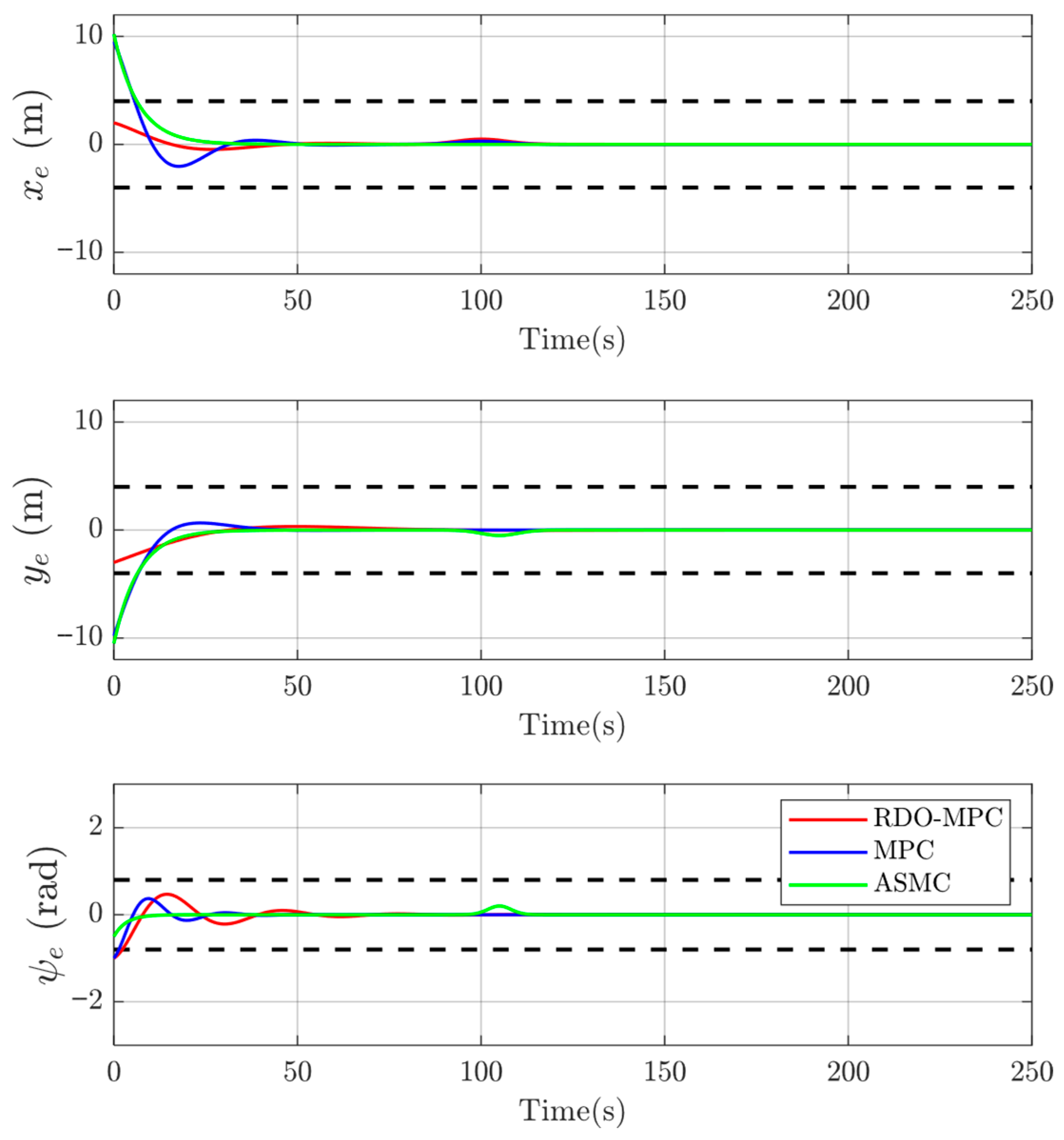
Figure 9 and Figure 10 present the trajectory tracking performance and pose tracking errors of the ASMC, MPC, and the proposed RDO-MPC algorithms under the continuously varying curvature path. As observed from Figure 9 and its enlarged view, at segments where the reference trajectory undergoes rapid continuous turns, the conventional MPC and ASMC methods exhibit noticeable lateral drift due to strong hydrodynamic nonlinear effects, making precise tracking difficult. In contrast, the proposed RDO-MPC algorithm closely follows the desired trajectory.
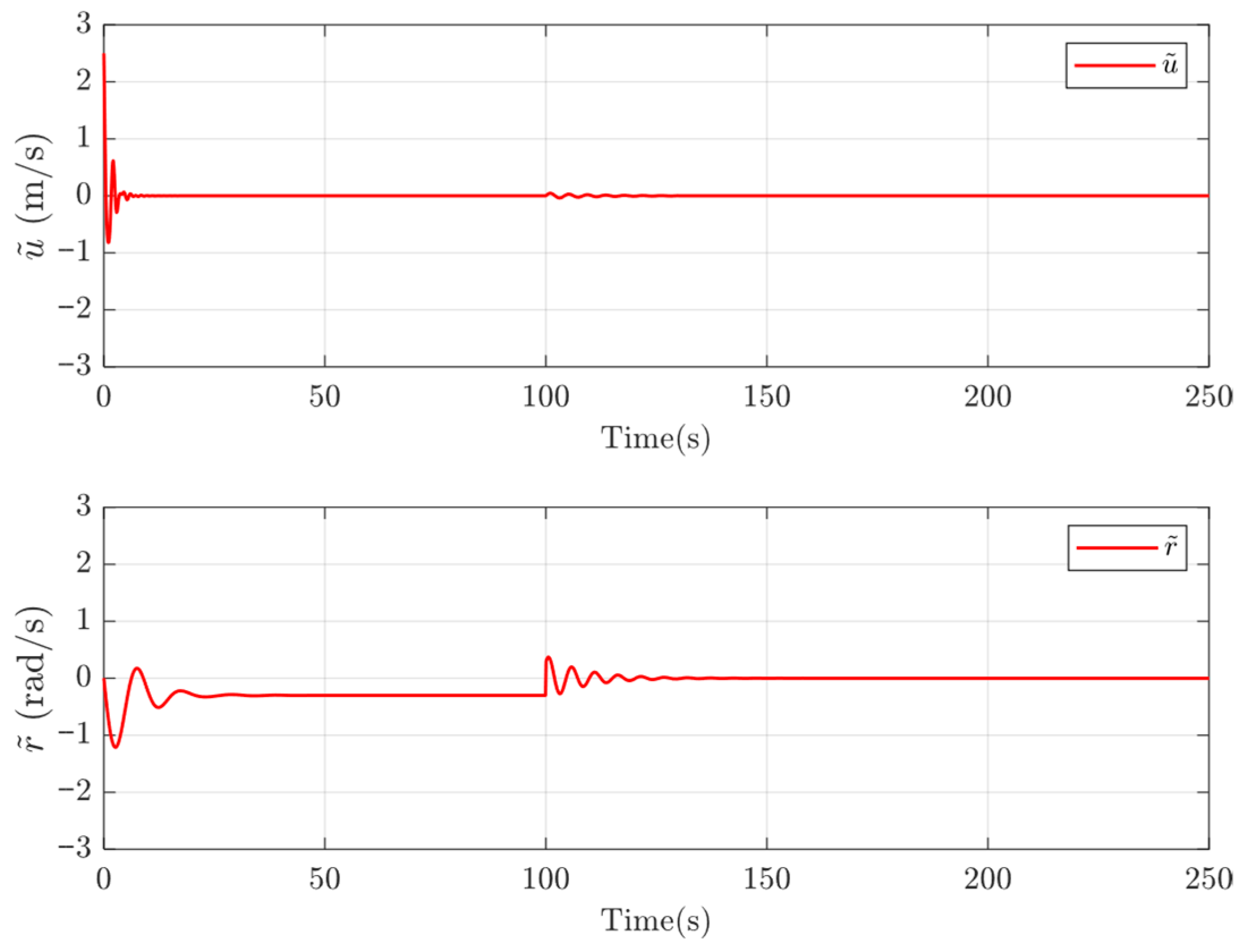
From the pose error curves in Figure 10, it can be seen that RDO-MPC achieves faster convergence and smaller overshoot both during the initial phase and at curvature transition points. The position error x e , y e and heading angle error ψ e are effectively confined within a reasonable range. Figure 11 shows the state observation errors under this complex operating condition. After experiencing short-term fluctuations caused by abrupt curvature changes, the surge velocity observation error u ˜ and yaw rate observation error r ˜ rapidly converge to a neighborhood around zero. These results demonstrate that the proposed RDO-MPC maintains excellent dynamic response performance and robustness even under challenging conditions characterized by strong hydrodynamic nonlinearities and significant drift tendencies.
The results of Test 2 further demonstrate that the advantage of the proposed method becomes more pronounced under dynamically varying curvature. Compared with MPC and ASMC, RDO-MPC maintains closer trajectory adherence, smaller pose deviations, and faster recovery of observation errors after transient fluctuations. This suggests that the proposed compensation-aware optimization framework is particularly beneficial when the USV is subjected to stronger nonlinear maneuvering demands.
The above results of Test 1 and Test 2 have demonstrated, through trajectory, pose-error, and state-observation responses, that the proposed RDO-MPC achieves superior tracking accuracy and robustness compared with MPC and ASMC. To further quantify this advantage from the optimization perspective, the cumulative value of the cost function defined in Equation (33) is calculated over the entire simulation horizon for the compared controllers. Since Equation (38) is the standard quadratic-programming reformulation of Equation (33), the reported cumulative cost corresponds to the same optimization objective. Here, k J k denotes the cumulative sum of the stage cost at all sampling instants, which reflects the overall trade-off among tracking accuracy, control smoothness, and constraint-handling performance throughout the complete control process.
As listed in Table 4, under the sinusoidal trajectory condition in Test 1, the cumulative cost of the proposed RDO-MPC is 753,200, which is 3.57% lower than that of MPC and 2.31% lower than that of ASMC. This indicates that, even in a relatively regular trajectory-tracking task, the proposed method achieves a better overall balance between tracking performance and control effort.
Under the time-varying curvature condition in Test 2, the cumulative cost of RDO-MPC is further reduced to 739,250, corresponding to improvements of 10.96% and 11.09% compared with MPC and ASMC, respectively. Since this scenario imposes stronger nonlinearity and more frequent curvature variations, the larger reduction in cumulative cost further confirms the advantage of the proposed RDO-MPC in handling complex maneuvering conditions. These results are consistent with the trajectory and error curves discussed above, and provide additional quantitative support for the effectiveness of the proposed method.
(3)
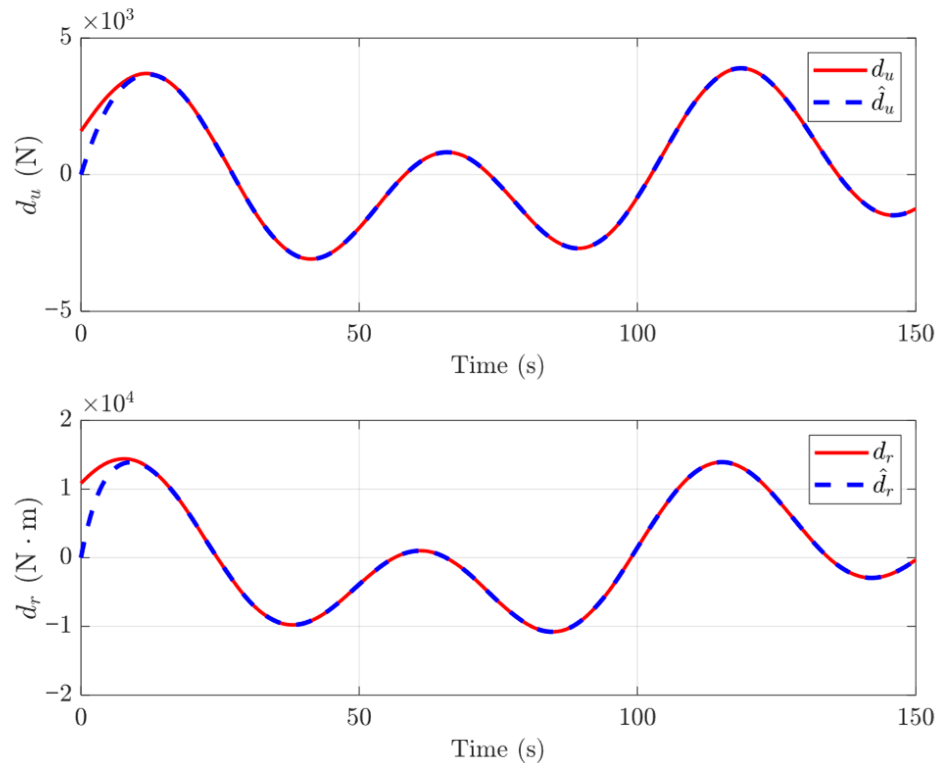
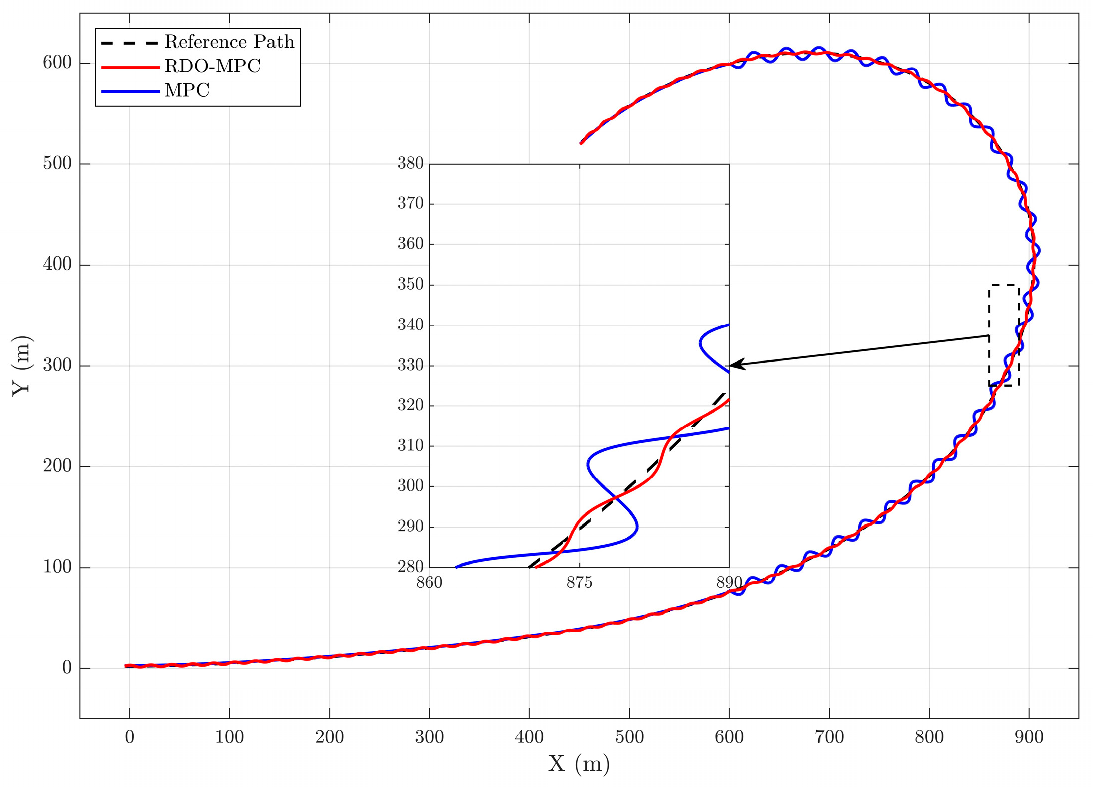
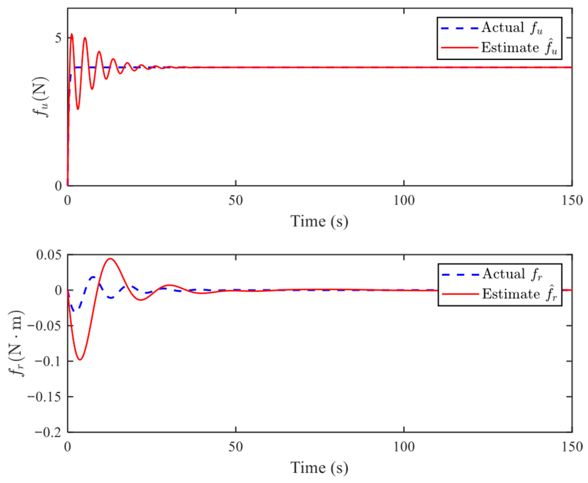
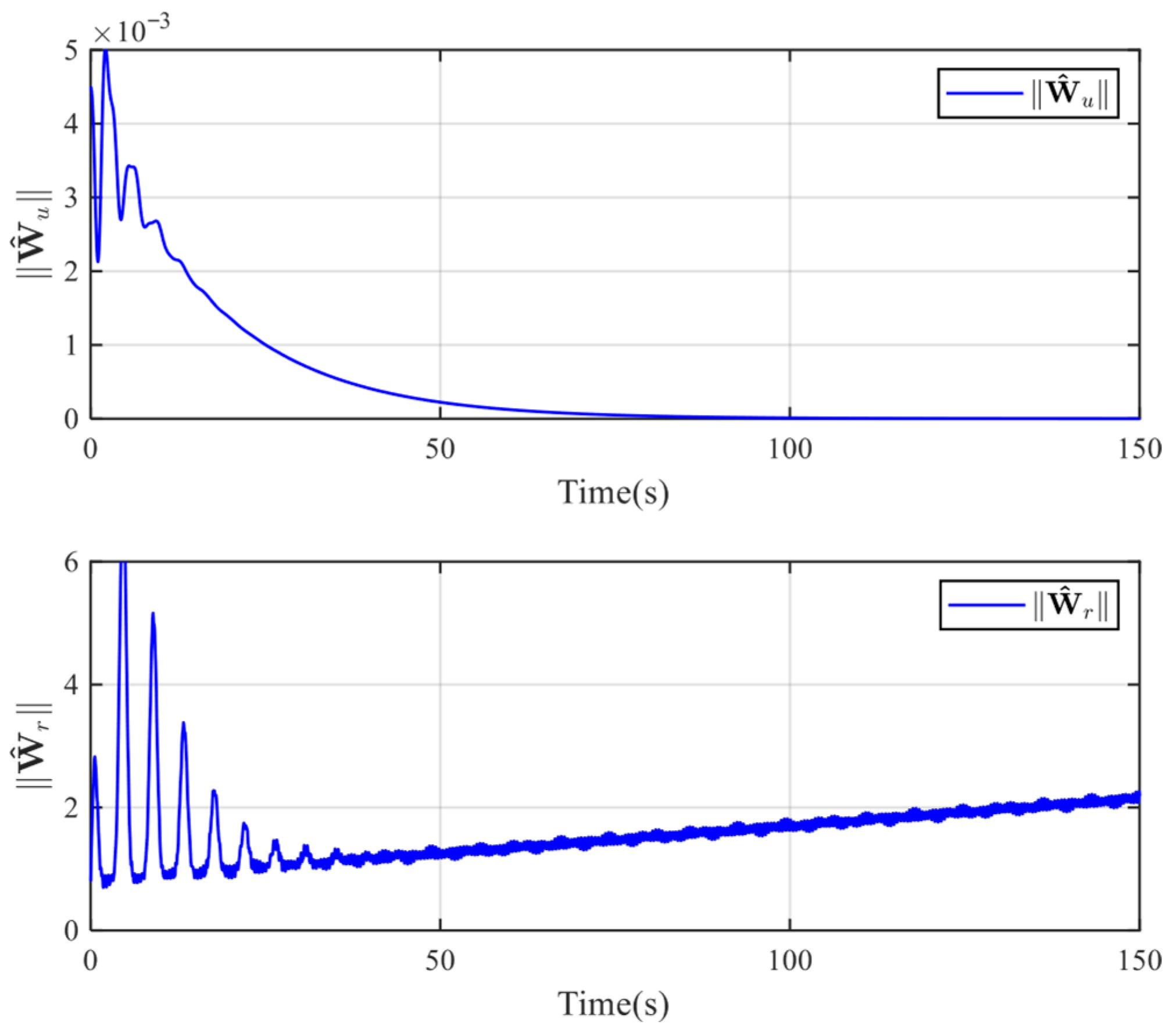
Test 3: This scenario is designed to evaluate the performance of the RBF neural network in online approximation and the effectiveness of sliding mode control in compensating for unknown disturbances and model uncertainties. In this case, a continuously increasing yaw rate is imposed, driving the USV into a sustained large-maneuver turning motion. During this process, as the sideslip angle increases, model uncertainties accumulate significantly. By focusing on the estimation outputs of the RBF network and the corresponding compensation effects, the role of the adaptive disturbance observer in improving the closed-loop system accuracy is demonstrated. In the following simulation, the trajectory tracking control gains k u = 4 and k r = 4 are specified, while the remaining parameters remain unchanged. The desired trajectory generated by the virtual vessel is defined as follows:
u d = 5   m / s r d = 0.1 e 0.004 t 0.1 r a d / s , t 0 .
The simulation duration is set to 150 s. For comparison, the conventional MPC controller and the proposed RDO-MPC are simulated under the same parameter variations and disturbance conditions.
Figure 12, Figure 13, Figure 14, Figure 15 and Figure 16 jointly illustrate the external tracking performance and actuator-feasible control behavior of the proposed method under large-maneuver conditions with parameter variation. As shown in Figure 12, when the sideslip angle increases and model uncertainty accumulates, the conventional MPC without RDO compensation exhibits obvious periodic oscillation and fails to maintain smooth trajectory tracking, whereas the proposed RDO-MPC still follows the desired path with satisfactory smoothness. Figure 13 and Figure 14 further corroborate this observation. The heading angle error ψ e of the conventional MPC exhibits sustained oscillations with nearly constant amplitude, while the position error x e , y e converges slowly and shows noticeable fluctuations. In contrast, all pose-related errors under the proposed RDO-MPC converge rapidly and smoothly to a neighborhood around zero, effectively eliminating steady-state errors. Figure 15 shows the actual control inputs of the RDO-MPC trajectory tracking controller, including the surge thrust τ u and yaw moment τ r . The results indicate that, even with the introduction of feedforward compensation to counteract unknown disturbances, the total control input remains strictly within the predefined physical amplitude constraints of the actuators. This effectively validates the safety guarantee provided by the dynamic constraint reconstruction module described earlier. Figure 16 compares the state observation errors of the two algorithms under parameter variations. In contrast to the persistent and severe oscillations observed in the conventional MPC, the observation errors u ˜ and r ˜ of the proposed RDO-MPC converge rapidly.
The internal working mechanism of the adaptive disturbance-observer-based compensation framework is further revealed by Figure 17, Figure 18 and Figure 19. Figure 17 shows that, for the lumped disturbances d u and d r acting on the USV, the estimated values d ^ u and d ^ r achieve high-precision online approximation, with the two curves almost completely overlapping. Figure 18 further illustrates the adaptive approximation effect of the proposed observer on model uncertainty and unknown disturbance under large-maneuver conditions. It can be observed that the RBFNN-based adaptive mechanism, together with the robust correction term, is able to reconstruct the dominant variation trend of the lumped uncertainty with satisfactory accuracy even when the parameter mismatch accumulates during turning. This result indicates that the observer does not merely provide a rough qualitative estimate, but can generate a practically usable disturbance-reconstruction signal for the subsequent compensation process. Figure 19 presents the time evolution of the adaptive RBFNN weights W ^ u and W ^ r during the large-maneuver tracking process. It can be seen that, after an initial transient learning stage, the weights gradually enter a bounded region and remain stable thereafter, rather than exhibiting unbounded growth or persistent divergence. It shows that the adaptive update law is numerically well behaved under sustained maneuvering and parameter-varying conditions, so that the online learning process does not introduce parameter drift, and the bounded weight evolution indicates that the neural-network approximation reaches a stable working regime after the initial adjustment, which is consistent with the boundedness analysis of the observer-adaptation mechanism established in Section 3.
Overall, Test 3 verifies the proposed framework from both external and internal perspectives, namely smooth large-maneuver trajectory tracking with actuator-feasible control, and reliable disturbance estimation with bounded adaptive evolution under parameter-varying conditions.

4.3. Sensitivity Analysis of the Soft-Constraint Penalty

To further verify the role of the soft-constraint term in Equation (33), a sensitivity study with respect to the penalty coefficient ρ ζ is carried out on the Test 3 trajectory. This scenario is selected because it imposes stronger constraint pressure on the controller and is therefore more suitable for examining how the soft optimization behaves when the admissible control region becomes tight. Four representative values, ρ ζ = 0 , 1, 10 and 100, are considered, while all other controller settings remain unchanged.
The trajectory-tracking results are shown in Figure 20. Although all cases remain globally stable and are able to follow the reference path, the local enlarged view reveals clear differences. When ρ ζ = 0 , the trajectory exhibits the most obvious oscillatory deviation, indicating that the optimizer relies excessively on slack activation when the soft penalty is absent. As ρ ζ increases to 1 and 10 , the local trajectory becomes noticeably smoother and closer to the reference path, showing that moderate slack penalization improves the balance between feasibility preservation and tracking accuracy. However, when ρ ζ = 100 , the local deviation increases again, implying that an excessively large penalty makes the optimization overly conservative and weakens the flexibility of soft-constraint adjustment.
Figure 21 and Figure 22 depict the tracking errors and the evolution of the normalized slack variable ζ , respectively. It is evident that the penalty coefficient ρ ζ regulates the soft-constraint mechanism, as slack usage decreases monotonically with an increasing ρ ζ . An unpenalized setup ρ ζ = 0 causes excessive constraint softening and high slack usage, deteriorating the transient response with severe oscillations and slow error attenuation. Conversely, an overly penalized setup ρ ζ = 100 forces ζ to zero, degrading into a conservative hard-constrained problem that amplifies residual errors. Moderate values, however, provide an optimal balance. Specifically, ρ ζ = 1 ensures the fastest and smoothest error convergence, while ρ ζ = 10 offers well-bounded tracking with limited slack activation. Ultimately, these results confirm that the soft optimization in Equation (33) provides a graceful adaptation mechanism for the proposed RDO-MPC under Test 3 conditions, successfully balancing tracking accuracy, constraint relaxation, and closed-loop smoothness.

5. Discussion

The simulation results presented in Section 4 provide a layered validation of the proposed RDO-MPC framework under constrained-water tracking conditions. Test 1 shows that the proposed method achieves smaller tracking deviation and better robustness than MPC and ASMC under a regular sinusoidal trajectory, while Test 2 further demonstrates that this advantage becomes more evident when the reference path contains continuously varying curvature and stronger maneuvering nonlinearity. In addition to the trajectory and pose-error curves, the cumulative performance-index comparison also confirms this trend quantitatively: in Test 1, the cumulative cost of the proposed RDO-MPC is reduced to 753,200, corresponding to decreases of 3.57% and 2.31% compared with MPC and ASMC, respectively, and in Test 2, the cumulative cost is further reduced to 739,250, with improvements of 10.96% and 11.09%, respectively. Test 3 provides additional evidence from the internal mechanism perspective. Under large-maneuver and parameter-varying conditions, the proposed framework maintains smoother trajectory evolution, faster error convergence, bounded observer errors, and actuator-feasible total control input, which indicates that the observer-compensation-constraint-reconstruction mechanism remains effective even when model uncertainty accumulates.
In addition to the above tracking and robustness results, the sensitivity analysis of the soft-constraint penalty further verifies an important design claim of the proposed method. By varying the penalty coefficient ρ ζ on the Test 3 trajectory, it is shown that the soft optimization in Equation (33) indeed provides a graceful adaptation mechanism when the admissible control region becomes tight. When ρ ζ = 0 , the optimizer relies excessively on slack activation, which leads to more obvious local trajectory oscillation and larger tracking-error fluctuations. As ρ ζ increases to moderate values, the controller achieves a better balance among tracking performance, constraint relaxation, and closed-loop smoothness. When ρ ζ becomes excessively large, the optimization behaves much more like a hard-constrained formulation, which reduces the flexibility of the soft-constraint mechanism and leads to a more conservative local response. Therefore, the new results not only complement the original simulation analysis, but also directly support the necessity of introducing the soft-constraint term into the proposed RDO-MPC framework.
From the viewpoint of control architecture, the main feature of the present work is not simply the combination of MPC, neural-network approximation, and sliding-mode compensation, but the explicit coupling between online disturbance compensation and constrained predictive optimization. In many conventional observer-assisted MPC schemes, the estimated disturbance is mainly used as a feedforward compensation term or as a correction to the nominal model, whereas in the present framework, the compensation demand is further fed back to the optimizer to reconstruct the admissible control region online. This design is particularly relevant for actuator-constrained USV systems because it allows disturbance rejection and input-feasibility preservation to be addressed within a coordinated framework rather than as two loosely connected modules. In this sense, the contribution of the proposed method lies not only in improving tracking performance, but also in providing a compensation-aware predictive-control structure that better matches the practical control requirements of underactuated USVs operating in constrained waters.
At the same time, the scope of the present study should be interpreted appropriately. The disturbance environment considered here is introduced through a lumped disturbance model combining current, wind, wave effects, parameter perturbation, and unmodeled nonlinear dynamics, and is intended to reflect representative coupled uncertainty in constrained waters rather than a site-specific sea-state reconstruction. In addition, because the considered USV is underactuated, the observer-based compensation is explicitly designed for the matched surge and yaw channels, while the lateral effect is handled implicitly through the coupled dynamics and the closed-loop tracking process. Although the current validation is mainly based on numerical simulations, the results consistently support the effectiveness of the proposed method in terms of tracking quality, robustness, observer convergence, and actuator-feasible control. More extensive benchmark comparisons with representative advanced frameworks and hardware-level validation will be further investigated in future work.

6. Conclusions

This paper proposed an RDO-MPC framework for trajectory tracking of an underactuated USV in constrained waters. By integrating predictive optimization, an RBFNN-based adaptive robust disturbance observer, and a compensation-aware dynamic constraint reconstruction mechanism, the proposed method explicitly coordinates disturbance rejection and actuator-feasible constrained control. Compared with conventional observer-assisted predictive control strategies, its main feature lies in feeding the disturbance-compensation demand back into the optimizer to update the admissible control region online. The simulation results verify the effectiveness of the proposed method under multiple representative scenarios. In Test 1, the cumulative performance index is reduced to 753,200, corresponding to decreases of 3.57% and 2.31% compared with MPC and ASMC, respectively. In Test 2, the cumulative cost is further reduced to 739,250, with improvements of 10.96% and 11.09%, respectively. In Test 3, the proposed framework maintains smoother trajectory evolution, faster error convergence, bounded observer errors, and actuator-feasible control behavior under large-maneuver and parameter-varying conditions. In addition, the sensitivity analysis of the soft-constraint penalty on the Test 3 trajectory confirms that the soft optimization in Equation (33) provides graceful adaptation when the admissible control region becomes tight, and that moderate values of ρ ζ provide a more favorable compromise between tracking performance and constraint relaxation.
While RDO-MPC exhibits promising performance in simulation environments, critical directions warrant further investigation: (1) enhanced modeling of coupled wind-wave-current disturbances through advanced multi-source interaction analysis; (2) hardware validation of algorithm robustness under real-world sensor noise and communication latency; (3) extension to distributed optimization frameworks for multi-USV collaborative operations; and (4) more systematic benchmark comparisons with representative advanced frameworks such as Tube MPC, Robust MPC, and ESO-based MPC, as well as hardware-in-the-loop or real-platform validation, will be considered in future work. These extensions could substantially improve the autonomy and operational safety of marine vehicle fleets in complex maritime environments.

Author Contributions

J.Z.: Writing—Original draft, Visualization, Validation, Software, Methodology, Formal analysis, Conceptualization. H.L.: Writing—Review and editing, Supervision, Methodology, Conceptualization. W.S.: Methodology, Writing—Review and editing, Supervision. A.L.: Methodology, Writing—Review and editing, Supervision. C.S.: Supervision, Writing—Review and editing. J.H.: Supervision, Writing—Review & editing. All authors have read and agreed to the published version of the manuscript.

Funding

This work was supported by the Jiangsu Province Graduate Practical Innovation Program [KYCX25_4397] and the Jiangsu Province Science and Technology Achievement Transformation Project [BA2023019].

Data Availability Statement

The original contributions presented in this study are included in the article. Further inquiries can be directed to the corresponding author. and confirm with author.

Conflicts of Interest

The authors declare that they have no known competing financial interests or personal relationships that could have appeared to influence the work reported in this paper.

Nomenclature

Main SymbolsMeaning
η = x , y , ψ T Inertial-frame position and heading vector
v = u , v , r T Body-fixed velocity vector
x , y Position coordinates in the inertial frame
ψ Heading angle
u Surge velocity
v Sway velocity
r Yaw rate
d X , t Lumped disturbance vector
d u , d v , d r Lumped disturbance components in surge, sway, and yaw directions
U m p c k Nominal control input
U c o m p k Feedforward compensation input

References

  1. Petrovski, A.; Radovanović, M. Application of detection reconnaissance technologies use by drones in collaboration with C4IRS for military interested. Contemp. Maced. Def. 2021, 21, 117–126. [Google Scholar]
  2. Han, S.; Sun, J.; Yan, L.; Ding, S.; Zhou, L. Research on effective trajectory planning, tracking, and reconstruction for USV formation in complex environments. Ocean Eng. 2025, 341, 122488. [Google Scholar] [CrossRef]
  3. Shang, X.; Zhang, G.; Lyu, H.; Tan, G. Research on Intelligent Navigation Technology: Intelligent Guidance and Path-Following Control of USVs. J. Mar. Sci. Eng. 2024, 12, 1548. [Google Scholar] [CrossRef]
  4. Argentim, L.M.; Rezende, W.C.; Santos, P.E.; Aguiar, R.A. PID, LQR and LQR-PID on a quadcopter platform. In Proceedings of the 2013 2nd International Conference on Informatics, Electronics and Vision (ICIEV), Dhaka, Bangladesh, 17–18 May 2013; IEEE: New York, NY, USA, 2013; pp. 1–6. [Google Scholar] [CrossRef]
  5. Qu, K.; Zhuang, W.; Wu, W.; Li, M.; Shen, X.; Li, X.; Shi, W. Stochastic Cumulative DNN Inference with RL-Aided Adaptive IoT Device-Edge Collaboration. IEEE Internet Things J. 2023, 10, 18000–18015. [Google Scholar] [CrossRef]
  6. Holkar, K.S.; Waghmare, L.M. An overview of model predictive control. Int. J. Control Autom. 2010, 3, 47–63. [Google Scholar]
  7. Raffo, G.V.; Gomes, G.K.; Normey-Rico, J.E.; Kelber, C.R.; Becker, L.B. A Predictive Controller for Autonomous Vehicle Path Tracking. IEEE Trans. Intell. Transp. Syst. 2009, 10, 92–102. [Google Scholar] [CrossRef]
  8. Wang, H.; Liu, B.; Ping, X.; An, Q. Path Tracking Control for Autonomous Vehicles Based on an Improved MPC. IEEE Access 2019, 7, 161064–161073. [Google Scholar] [CrossRef]
  9. Ostafew, C.J.; Schoellig, A.P.; Barfoot, T.D. Robust constrained learning-based NMPC enabling reliable mobile robot path tracking. Int. J. Robot. Res. 2016, 35, 1547–1563. [Google Scholar] [CrossRef]
  10. Backman, J.; Oksanen, T.; Visala, A. Navigation system for agricultural machines: Nonlinear model predictive path tracking. Comput. Electron. Agric. 2012, 82, 32–43. [Google Scholar] [CrossRef]
  11. Zhou, X.; Wu, Y.; Huang, J. MPC-based path tracking control method for USV. In Proceedings of the 2020 Chinese Automation Congress (CAC), Shanghai, China, 6–8 November 2020; Springer Nature: Berlin/Heidelberg, Germany, 2020; pp. 1669–1673. [Google Scholar] [CrossRef]
  12. Zhao, B.; Zhang, X.; Liang, C.; Han, X. An Improved Model Predictive Control for Path-Following of USV Based on Global Course Constraint and Event-Triggered Mechanism. IEEE Access 2021, 9, 79725–79734. [Google Scholar] [CrossRef]
  13. Luo, Q.; Wang, H.; Li, N.; Su, B.; Zheng, W. Model-free Predictive Trajectory Tracking Control and Obstacle Avoidance for Unmanned Surface Vehicle with Uncertainty and Unknown Disturbances via Model-free Extended State Observer. Int. J. Control Autom. Syst. 2024, 22, 1985–1997. [Google Scholar] [CrossRef]
  14. Zhao, S.; Mu, J.; Liu, H.; Sun, Y.; Cajo, R. Heading control of USV based on fractional-order model predictive control. Ocean Eng. 2025, 322, 120476. [Google Scholar] [CrossRef]
  15. Li, A.; Hu, X.; Dong, K.; Xiao, B. An improved MPSP-based path-following control method for USV with input disturbances. Optim. Control Appl. Methods 2025, 46, 440–458. [Google Scholar] [CrossRef]
  16. Zhang, L.; Zhang, S.; Du, Z.; Li, H.; Gan, L.; Li, X. Adaptive trajectory tracking of the unmanned surface vessel based on improved AC-MPC method. Ocean Eng. 2025, 322, 120455. [Google Scholar] [CrossRef]
  17. Lopez, B.T.; Slotine, J.-J.E.; How, J.P. Dynamic Tube MPC for Nonlinear Systems. In Proceedings of the 2019 American Control Conference (ACC), Philadelphia, PA, USA, 10–12 July 2019; IEEE: New York, NY, USA, 2019; pp. 1655–1662. [Google Scholar] [CrossRef]
  18. Fossen, T.I. Handbook of Marine Craft Hydrodynamics and Motion Control; John Wiley & Sons: Hoboken, NJ, USA, 2011. [Google Scholar]
  19. Hasselmann, K.; Barnett, T.P.; Bouws, E.; Carlson, H.; Cartwright, D.E.; Enke, K.; Ewing, J.A.; Gienapp, A.; Hasselmann, D.E.; Kruseman, P.; et al. Measurements of wind-wave growth and swell decay during the Joint North Sea Wave Project (JONSWAP). Ergaenzungsheft Zur Dtsch. Hydrogr. Z. Reihe A 1973. Available online: https://pure.mpg.de/view/item_3262854 (accessed on 19 April 2026).
  20. Tamekue, C.; Ching, S. Control analysis and synthesis for general control-affine systems. arXiv 2025, arXiv:2503.05606. [Google Scholar] [CrossRef]
  21. Limon, D.; Alamo, T.; Salas, F.; Camacho, E. On the stability of constrained MPC without terminal constraint. IEEE Trans. Autom. Control 2006, 51, 832–836. [Google Scholar] [CrossRef]
  22. Yin, Y.; Liu, J.; Sanchez, J.A.; Wu, L.; Vazquez, S.; Leon, J.I.; Franquelo, L.G. Observer-Based Adaptive Sliding Mode Control of NPC Converters: An RBF Neural Network Approach. IEEE Trans. Power Electron. 2019, 34, 3831–3841. [Google Scholar] [CrossRef]
  23. Chen, W.-H.; Yang, J.; Guo, L.; Li, S. Disturbance-Observer-Based Control and Related Methods—An Overview. IEEE Trans. Ind. Electron. 2016, 63, 1083–1095. [Google Scholar] [CrossRef]
  24. Angeli, D.; Sontag, E.; Wang, Y. A characterization of integral input-to-state stability. IEEE Trans. Autom. Control 2000, 45, 1082–1097. [Google Scholar] [CrossRef]
  25. Zhu, Y.; Qiao, J.; Guo, L. Adaptive Sliding Mode Disturbance Observer-Based Composite Control with Prescribed Performance of Space Manipulators for Target Capturing. IEEE Trans. Ind. Electron. 2019, 66, 1973–1983. [Google Scholar] [CrossRef]
  26. Lorenzen, M.; Cannon, M.; Allgöwer, F. Robust MPC with recursive model update. Automatica 2019, 103, 461–471. [Google Scholar] [CrossRef]
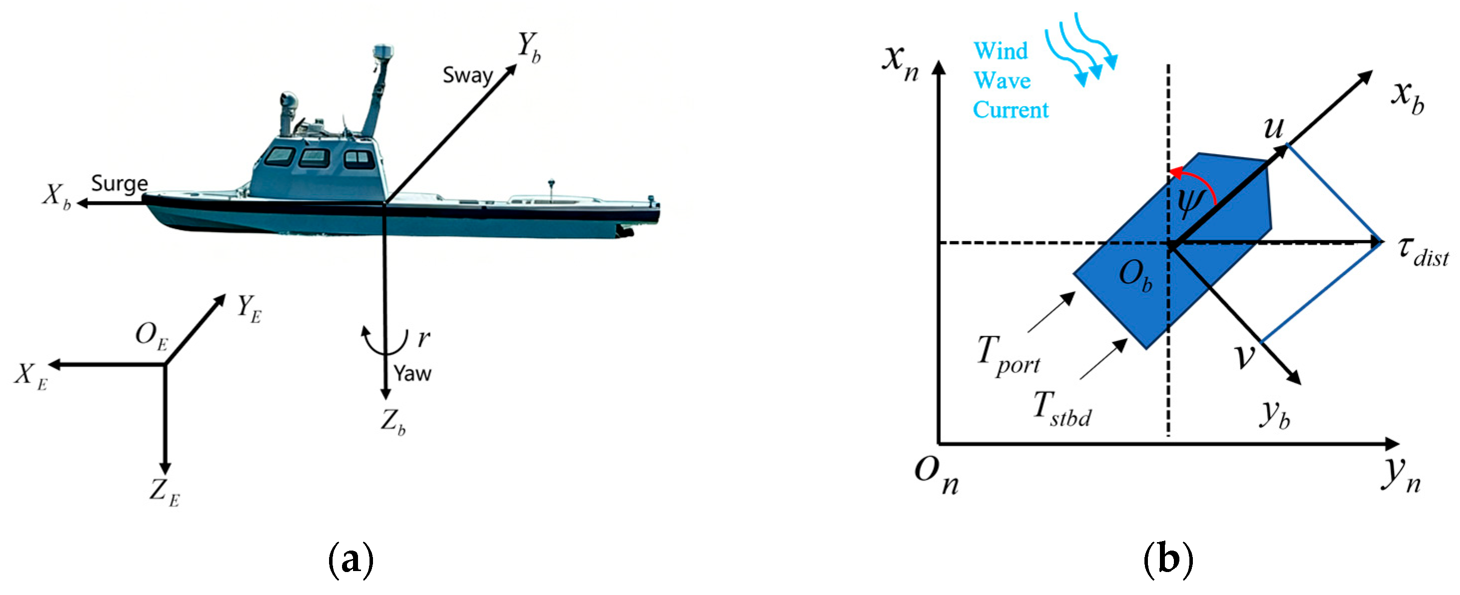
Figure 1. USV configuration and coordinate definitions: (a) physical configuration of the USV and object-fixed motion directions; (b) inertial frame, object-fixed frame, and 3-DOF motion variables.
Jmse 14 00757 g001
Figure 2. Basic Principles of MPC.
Jmse 14 00757 g002
Figure 3. Schematic diagram of RBF neural network structure.
Jmse 14 00757 g003
Figure 4. RDO-MPC System Framework Diagram.
Jmse 14 00757 g004
Figure 5. Path tracking without parameter perturbation.
Jmse 14 00757 g005
Figure 6. Path tracking with parameter perturbation.
Jmse 14 00757 g006
Figure 7. Pose tracking error of unmanned ships with constraints.
Jmse 14 00757 g007
Figure 8. State observation error quantity.
Jmse 14 00757 g008
Figure 9. Path tracking results with curvature variation.
Jmse 14 00757 g009
Figure 10. Pose error due to curvature variation.
Jmse 14 00757 g010
Figure 11. State observation error quantity of curvature variation.
Jmse 14 00757 g011
Figure 12. Path tracking results after parameter changes.
Jmse 14 00757 g012
Figure 13. The heading angle error before and after adding RDO disturbance compensation.
Jmse 14 00757 g013
Figure 14. Positioning error of the USV after parameter changes.
Jmse 14 00757 g014
Figure 15. Output of the path tracking controller.
Jmse 14 00757 g015
Figure 16. State estimation error quantity of path tracking after parameter changes.
Jmse 14 00757 g016
Figure 17. Disturbance estimation for USV.
Jmse 14 00757 g017
Figure 18. Adaptive effect approximate estimation of uncertainty and unknown disturbance for USV model.
Jmse 14 00757 g018
Figure 19. Adaptive RBFNN weight changes.
Jmse 14 00757 g019
Figure 20. Trajectory tracking results under different soft-constraint penalty coefficients.
Jmse 14 00757 g020
Figure 21. Tracking errors under different soft-constraint penalty coefficients.
Jmse 14 00757 g021
Figure 22. Evolution of the normalized slack variable ζ under different soft-constraint penalty coefficients.
Jmse 14 00757 g022
Table 1. Main parameters of the self-developed USV and the dynamic model parameters used in this study. The values are obtained from the design specifications, measured platform data, and model settings of the laboratory-developed USV.
ParametersNumerical ValueParametersNumerical ValueParametersNumerical Value
m 9800 kg N r 4500 kg × m2/s Y v v 3800 kg/m
L 9.65 m X u ˙ 490 kg N r r 35,000 kg × m2
d 0.64 m Y v ˙ 10,972 kg I z z 36,574 kg × m2
X u 200 kg/s N r ˙ 7300 kg × m2
Y v 3500 kg/s X u u 95 kg/m
Table 2. Actuator constraint parameters of the self-developed USV propulsion system. The values are determined according to the operating limits and safety constraints of the twin-thruster propulsion system used in this study.
Physical ConstraintsNumerical Value
Maximum longitudinal thrust τ u , max 13,000 N
Minimum longitudinal thrust τ u , min −10,000 N
Maximum turning moment of the rudder τ r , max 46,600 N × m
Minimum turning moment of the rudder τ r , min −46,600 N × m
Thrust rate limit Δ τ u 3000 N × s−1
Torque rate of change limit Δ τ r 5000 N × m · s−1
Table 3. Key RMPC parameters and weighting matrices used in the simulation study.
TypeNumerical Value
Sampling time T s 0.1 s
Prediction time domain N p 30
Control of the time domain N c 5
State error weight matrix Q diag 10 3 , 10 3 , 5 × 10 3
Control the incremental weight matrix R diag [ 0.1 , 0.1 , 0.1 ]
Table 4. Comparison of cumulative performance index values in Test 1 and Test 2 based on Equation (33).
ScenarioController Cumulative   Cost   k J k Relative Improvement
Test 1MPC781,050/
Test 1ASMC771,000/
Test 1RDO-MPC753,2003.57% vs. MPC/2.31% vs. ASMC
Test 2MPC830,250/
Test 2ASMC831,450/
Test 2RDO-MPC739,25010.96% vs. MPC/11.09% vs. ASMC
Disclaimer/Publisher’s Note: The statements, opinions and data contained in all publications are solely those of the individual author(s) and contributor(s) and not of MDPI and/or the editor(s). MDPI and/or the editor(s) disclaim responsibility for any injury to people or property resulting from any ideas, methods, instructions or products referred to in the content.