Advances in Imputation Strategies Supporting Peak Storm Surge Surrogate Modeling
Abstract
1. Introduction
2. Problem Formulation
3. Database Description
4. Surrogate Modeling Overview
4.1. Database Imputation
4.2. Surrogate Model Development
4.2.1. Overview of Data-Driven Predictive Model Formulation
4.2.2. Classification and Regression Surrogate Model Details
4.2.3. Combination of Individual Surrogate Model Predictions
- The always-wet nodes (inundated across the entire database), with no missing information. These will be denoted as class. The node condition classification for them is based entirely on Ss.
- The modified problematic nodes for which imputation was needed, and that imputation led to sufficiently large values of or . These will be denoted as class.
- The remaining nodes, for which imputation was needed, but that imputation did not lead to significant misclassification. These will be denoted as class.
4.3. Surrogate Model Validation
5. Imputation Based on Spatial Interpolation
5.1. Imputation Using kNN with Enhanced Hydraulic Connectivity
5.2. Imputation Using GPI with Adaptive Covariance Tapering
5.3. Computational Complexity and Scalability of Spatial Interpolation Techniques
6. Imputation Based on Data Completion
6.1. Motivation for Imputation Utilizing Data Completion
6.2. Imputation Using PPCA
6.3. Two-Stage Imputation Combining Spatial Interpolation and Data Completion Techniques
6.4. Computational Complexity and Scalability of PPCA Imputation
7. Illustrative Case Study
7.1. Variants Examined
7.2. Imputation Results
7.3. Surrogate Model Performance for the Entire Domain
7.4. Surrogate Model Performance for the Subdomain
7.5. Trends for Distribution of Errors
8. Conclusions
- As reported in previous studies, the best overall performance can be established by combining a regression and a classification surrogate models, with the regression model developed utilizing directly the imputed database without any corrections.
- Spatial interpolation using response-based connectivity information can better capture discontinuous patterns in surge responses, demonstrating superiority in supporting surrogate model development with improved predictive accuracy at problematic nodes. Note that such nodes can be identified by the larger surge gaps in the original data.
- Imputation utilizing GPI is a viable alternative (compared to kNN) imputation strategy based on spatial interpolation, and can better capture the global surge trends, offering superior overall performance. However, it cannot capture discontinuous patterns in surge responses, and extending GPI using response-based connectivity information within the covariance kernel is not straightforward. Nevertheless, this is a topic that should be investigated in the future.
- Data completion imputation for the peak-surge demonstrates very poor performance, originating from the fact that for many (predominantly dry) nodes, very limited information is available in the original database to establish the underlying patterns to fill in the missing data. An enrichment stage of the original data, using spatial interpolation in the first stage, is needed for data completion to offer any advantages.
- The two-stage imputation strategy combining spatial interpolation (stage 1) with data completion (stage 2) for the misclassified instances from the first stage offers additional robustness in the predictions and has the potential to further improve accuracy compared to the approach implemented in stage 1. The degree of improvement depends on the quality of information available for the second stage, which is a function of both the size of the database as well as the degree of enrichment established in the first stage for the originally predominantly dry nodes.
Author Contributions
Funding
Institutional Review Board Statement
Informed Consent Statement
Data Availability Statement
Acknowledgments
Conflicts of Interest
Nomenclature
| Terminologies | |
| always-wet nodes | Nodes that have been inundated across all storms in the database |
| once-dry nodes | Nodes that have been dry at least once (i.e., with missing data) in the database |
| problematic nodes | Nodes whose imputed pseudo-surge values were misclassified (above node elevations) at least once |
| pseudo-surge database | Database in which all missing data are filled with pseudo-surge values through imputation |
| corrected pseudo-surge database | Database in which all missing data are filled with pseudo-surge values through imputation, with any misclassified pseudo-surge values corrected to be below node elevations |
| Notations | |
| Group of problematic nodes | |
| Modified group containing only problematic nodes with high misclassification rates and large discrepancies from node elevations | |
| Class of always-wet nodes | |
| Class of once-dry nodes whose pseudo-surge values exhibit high misclassification rates and large discrepancies from node elevations (corresponding to ) | |
| Class of once-dry nodes whose pseudo-surge values exhibit low misclassification rates and small discrepancies from node elevations | |
| Ss | Regression surrogate model used to predict surge levels |
| Sc | Classification surrogate model used to predict node condition (dry or wet) |
| Df | Full domain containing 1,179,179 nodes |
| Ds | Subdomain of the full domain (Df) containing 200,200 nodes |
| Validation metrics | |
| Averaged surge score for the ith node across all storms in the database | |
| Misclassification rate for the ith node across all storms in the database | |
| False positive rate for the ith node across all storms in the database | |
| False negative rate for the ith node across all storms in the database | |
| Averaged validation metric across all nodes ( = , , , or ) | |
| Examined imputation strategies | |
| kNN | Spatial interpolation-based imputation using weighted k-nearest neighbor (kNN) interpolation, where the connectivity of original numerical model grids is considered as hydraulic connectivity |
| kNNrc | Spatial interpolation-based imputation using weighted kNN interpolation, where response similarity between nodes is considered as hydraulic connectivity, as proposed in this study |
| GPI | Spatial interpolation-based imputation using Gaussian Process interpolation (GPI) with adaptive covariance tapering scheme |
| PPCA | Data completion-based imputation using probabilistic principal component Analysis (PPCA) |
Appendix A. Review of GP-Based Regression Ss Metamodel
- Step 1: Dimensionality reduction. To address the high dimensionality of the output z, principal component analysis (PCA) [59] is used as a dimensionality reduction technique [12]. PCA is performed on Z and identifies, through a linear projection matrix , a small number of latent outputs (principal components) that best explain the variance of the original observation matrix Z, with . For each component, it also provides the vector of observations whose hth row corresponds to the latent output for the hth storm, and its relative importance ωt corresponding to the portion of the variance of the original observation matrix Z that can be explained by the respective component. The latter information is leveraged to select the number of principal components to retain [59]. The PCA transformation also utilizes the mean (across the storm database) of the observations for each , denoted herein as μi. This simply corresponds to the mean of each column of Z.
- Step 2: Principal component GP calibration. For each of the principal components, a separate GP is developed using input–output observation pair X-. This is accomplished through the formulation reviewed in Appendix C for definitions , , , and with and . The GP provides the predictive mean and variance for each latent component given by Equations (A6) and (A7), respectively. Note that the dimensionality reduction established in Step 2 accommodates a computationally efficient GP calibration separately for each principal component, since is typically small (relative to both n and, especially, nz).
- Step 3: Storm surge predictions. Combining the predictions for all principal components, the metamodel approximation for the storm surge is obtained using the linear PCA transformation. Adopting notation to denote the element of a matrix (corresponding to the ith row and tth column), the mean and variance predictions for the ith node are as follows [12]:
Appendix B. Review of GP-Based Classification Sc Metamodel
- Step 1: Dimensionality reduction and projection to continuous output. To address the high dimensionality of the output y and accommodate a projection to a continuous space, logistic principal component analysis (LPCA) [60] is used as a dimensionality reduction technique [23]. LPCA is performed by maximizing the likelihood of observations Y given the compact representation for the natural parameter (log-odds) vector θ of the underlying logistic function describing y [60]. It identifies a small number of latent outputs along with the projection matrix , the bias for each component, and the latent observation matrix whose hth row corresponds to the latent output for the hth storm. The value of can be selected based on parametric sensitivity analysis to avoid overfitting [23]. The latent outputs describing the natural parameters correspond to a continuous variable, even though the original data corresponded to a binary variable. This facilitates the use of a regression surrogate model for predicting in Step 2.
- Step 2: Principal component GP calibration. For each of the principal components, a separate GP is developed using input–output observation pair X-. This is accomplished through the formulation reviewed in Appendix C for definitions , , , and , with and . The GP provides the predictive mean given by Equation (A6). Note that the dimensionality reduction established in Step 2 accommodates a computationally efficient GP calibration separately for each principal component, since is typically very small (relative to both n and, especially, nz).
- Step 3: Classification predictions. Combining the predictions for all principal components, the metamodel approximation for the inundation state for the ith node is first established by obtaining the natural parameter approximation for that node through the linear transformation:
Appendix C. Review of GP Formulation
Appendix D. Weighted k-Nearest Neighbor (kNN) Calibration
Appendix E. Adaptive Taper Selection Using Inducing Points
- Step 1: Check total number of neighbors. Evaluate the appropriate correction to obtain the most benefits for the overall number of non-zero elements. For the inducing points, perform the following operations: [23]:
- Step 2: Adjust most influential taper. Depending on the outcome of Equation (A11).
- Step 3: Taper range adjustment. Compute the taper range adjustment for the mth node, so that . This is achieved by ordering the elements , then randomly choosing a number, denoted φadj, between the and ordered values. Finally, update the mth taper range to be .
- Step 4: Update taper vector and taper thresholds. The new taper range vector φ(k) is obtained by replacing with . If , proceed to Step 5 and update . Otherwise, update the taper threshold matrix based on the new by setting (updating the mth row) and (updating the id(m)th column), and proceed to the next iteration by returning to Step 1.
- Step 5: Use interpolation to update entire vector. Update the entire taper based on projection mapping . This provides the taper ranges for the remaining points (i.e., non-inducing points) based on the taper ranges for the inducing points.
- Step 6: Global update of taper thresholds and number of non-zeros. Using the new vector , calculate and the new number of non-zero elements for each inducing point by identifying the entries satisfying .
- Step 7: Assess stopping criteria. If , set and stop iterating since the allowable computation burden has been exceeded. If , examine the convergence criteria. For the inducing points, examine the following conditions:If both conditions are satisfied, the algorithm has convergence and iterations may stop (and set ). Otherwise, set and proceed to the next iteration by returning to Step 1.
Appendix F. Adaptive Taper Selection Using Inducing Points
- Step 1: Perform M-IAT. Perform M-IAT using as the current set of inducing points. If , then the taper range vector φ[l] used within M-IAT may be initialized based on the taper range values identified at the previous iteration of IIP.
- Step 2: Check convergence. Estimate the number of non-zero elements for all nodes in the domain by identifying nodes satisfying . If or is satisfied, convergence has been achieved and is the final set of inducing points. Otherwise, proceed to Step 4.
- Step 3: Select new inducing points. The remaining nodes (i.e., non-inducing points) are separated into two groups: (a) those for which there are sufficiently too many non-zero elements (i.e., ); and (b) those for which there are sufficiently too few non-zero elements (i.e., ). These groups are denoted and , respectively, and contain nG+ and nG– nodes, respectively. Separately, perform clustering within each group ( and ) and select the number of clusters (within each group) to be proportional to the number of total nodes in the group while incorporating the weight cn. This yields clusters for and clusters for . The nG+ nodes within are clustered into n+ clusters based on spatial location, and the worst-performing node (i.e., the node with the largest discrepancy ) within each cluster is selected as the representative point to be added to the existing set of inducing points. Denote these nodes . Similarly, the nG– nodes within are clustered into n– clusters based on spatial location, and the worst-performing node within each cluster is selected as the representative point to be added to the existing set of inducing points. Denote these nodes . To obtain the updated set of inducing points, augment the existing set such that . The new set of inducing points contains nodes. Finally, set and proceed to the next iteration by returning to Step 1.
Appendix G. Performance of the Regression Surrogate Model Developed Based on the Pseudo-Surge Database Without Correction
| Pseudo-Surge Database (Ss Only) | ||||||
|---|---|---|---|---|---|---|
| kNN | kNNrc | PPCA | kNN-PPCA | kNNrc-PPCA | ||
| All nodes | 13.39 | 13.90 | 9.25 | 7.91 | 7.98 | |
| Once-dry | 19.08 | 20.28 | 8.93 | 6.08 | 6.22 | |
| Surge gap> (m) | 0.25 | 59.78 | 72.37 | 5.39 | 4.11 | 4.90 |
| 0.5 | 70.61 | 88.33 | 4.68 | 3.64 | 4.85 | |
| 0.75 | 87.09 | 106.73 | 4.72 | 3.73 | 5.30 | |
| 1 | 109.14 | 122.55 | 5.26 | 4.21 | 5.82 | |
| 1.5 | 139.46 | 142.92 | 7.95 | 6.43 | 7.67 | |
| Node groups | 38.95 | 36.06 | 9.03 | 7.88 | 7.73 | |
| 5.04 | 5.16 | 7.30 | 4.82 | 4.88 | ||
| Pseudo-Surge Database (Ss Only) | ||||||
|---|---|---|---|---|---|---|
| kNN | kNNrc | PPCA | kNN-PPCA | kNNrc-PPCA | ||
| All nodes | 7.19 | 7.68 | 10.82 | 3.70 | 4.17 | |
| Once-dry | 17.22 | 18.38 | 25.99 | 8.79 | 9.91 | |
| Surge gap> (m) | 0.25 | 46.94 | 47.91 | 19.90 | 11.68 | 15.86 |
| 0.5 | 53.76 | 55.55 | 18.12 | 11.34 | 17.78 | |
| 0.75 | 63.20 | 65.39 | 17.94 | 12.09 | 20.34 | |
| 1 | 71.31 | 74.12 | 18.81 | 12.99 | 21.25 | |
| 1.5 | 72.73 | 78.47 | 23.42 | 15.48 | 21.87 | |
| Node groups | 35.15 | 32.99 | 27.33 | 15.15 | 16.33 | |
| 4.55 | 4.38 | 2.97 | 4.36 | 4.23 | ||
| Pseudo-Surge Database (Ss Only) | ||||||
|---|---|---|---|---|---|---|
| kNN | kNNrc | PPCA | kNN-PPCA | kNNrc-PPCA | ||
| All nodes | 6.46 | 7.00 | 10.36 | 2.96 | 3.47 | |
| Once-dry | 15.61 | 16.90 | 25.02 | 7.14 | 8.39 | |
| Surge gap> (m) | 0.25 | 46.79 | 47.81 | 19.85 | 11.46 | 15.71 |
| 0.5 | 53.65 | 55.49 | 18.06 | 11.16 | 17.67 | |
| 0.75 | 63.12 | 65.34 | 17.87 | 11.93 | 20.23 | |
| 1 | 71.26 | 74.09 | 18.73 | 12.85 | 21.12 | |
| 1.5 | 72.73 | 78.47 | 23.33 | 15.37 | 21.74 | |
| Node groups | 34.28 | 32.18 | 26.40 | 14.18 | 15.41 | |
| 2.41 | 2.26 | 1.36 | 2.25 | 2.16 | ||
| Pseudo-Surge Database (Ss Only) | ||||||
|---|---|---|---|---|---|---|
| kNN | kNNrc | PPCA | kNN-PPCA | kNNrc-PPCA | ||
| All nodes | 0.73 | 0.68 | 0.46 | 0.74 | 0.70 | |
| Once-dry | 1.61 | 1.48 | 0.97 | 1.65 | 1.53 | |
| Surge gap> (m) | 0.25 | 0.15 | 0.10 | 0.06 | 0.22 | 0.15 |
| 0.5 | 0.11 | 0.06 | 0.06 | 0.18 | 0.11 | |
| 0.75 | 0.08 | 0.05 | 0.07 | 0.16 | 0.12 | |
| 1 | 0.05 | 0.03 | 0.08 | 0.14 | 0.13 | |
| 1.5 | 0.01 | 0.01 | 0.09 | 0.11 | 0.13 | |
| Node groups | 0.87 | 0.81 | 0.93 | 0.97 | 0.91 | |
| 2.14 | 2.13 | 1.61 | 2.12 | 2.07 | ||
| Pseudo-Surge Database (Ss Only) | ||||||||
|---|---|---|---|---|---|---|---|---|
| kNN | kNNrc | GPI | PPCA | kNN-PPCA | kNNrc-PPCA | GPI-PPCA | ||
| All nodes | 26.31 | 31.17 | 29.54 | 11.11 | 9.96 | 10.13 | 9.91 | |
| Once-dry | 48.82 | 61.01 | 57.15 | 9.78 | 7.22 | 7.54 | 7.43 | |
| Surge gap> (m) | 0.25 | 108.97 | 151.33 | 129.24 | 4.73 | 3.75 | 5.04 | 3.92 |
| 0.5 | 118.19 | 164.75 | 140.34 | 3.96 | 3.21 | 4.78 | 3.37 | |
| 0.75 | 131.17 | 177.32 | 153.55 | 3.62 | 2.98 | 4.76 | 3.11 | |
| 1 | 145.46 | 178.84 | 165.69 | 3.73 | 3.01 | 4.60 | 3.17 | |
| 1.5 | 177.34 | 190.90 | 195.68 | 5.88 | 4.66 | 5.42 | 5.09 | |
| Node groups | 87.01 | 104.95 | 84.83 | 10.28 | 7.86 | 8.45 | 8.22 | |
| 6.93 | 6.87 | 6.64 | 6.49 | 6.60 | 6.55 | 6.27 | ||
| Pseudo-Surge Database (Ss Only) | ||||||||
|---|---|---|---|---|---|---|---|---|
| kNN | kNNrc | GPI | PPCA | kNN-PPCA | kNNrc-PPCA | GPI-PPCA | ||
| All nodes | 13.83 | 13.55 | 15.01 | 9.49 | 3.77 | 4.77 | 4.40 | |
| Once-dry | 34.73 | 34.03 | 37.68 | 23.81 | 9.41 | 11.90 | 11.00 | |
| Surge gap> (m) | 0.25 | 76.92 | 78.04 | 79.88 | 15.58 | 11.29 | 19.14 | 11.19 |
| 0.5 | 83.44 | 85.15 | 86.48 | 13.86 | 10.87 | 20.20 | 10.33 | |
| 0.75 | 87.79 | 89.20 | 89.31 | 12.81 | 10.76 | 20.51 | 9.81 | |
| 1 | 88.66 | 89.75 | 89.41 | 13.34 | 11.05 | 18.59 | 9.94 | |
| 1.5 | 87.58 | 88.15 | 88.15 | 18.53 | 14.16 | 15.26 | 13.74 | |
| Node groups | 62.61 | 58.46 | 56.41 | 27.14 | 15.18 | 19.35 | 16.27 | |
| 4.14 | 3.93 | 3.51 | 2.00 | 3.83 | 3.70 | 3.32 | ||
| Pseudo-Surge Database (Ss Only) | ||||||||
|---|---|---|---|---|---|---|---|---|
| kNN | kNNrc | GPI | PPCA | kNN-PPCA | kNNrc-PPCA | GPI-PPCA | ||
| All nodes | 13.32 | 13.09 | 14.60 | 9.29 | 3.25 | 4.29 | 3.97 | |
| Once-dry | 33.52 | 32.95 | 36.75 | 23.39 | 8.19 | 10.79 | 10.00 | |
| Surge gap> (m) | 0.25 | 76.79 | 77.95 | 79.84 | 15.50 | 11.08 | 18.99 | 11.07 |
| 0.5 | 83.35 | 85.08 | 86.47 | 13.78 | 10.69 | 20.07 | 10.23 | |
| 0.75 | 87.74 | 89.15 | 89.30 | 12.72 | 10.61 | 20.38 | 9.71 | |
| 1 | 88.63 | 89.73 | 89.41 | 13.25 | 10.91 | 18.46 | 9.85 | |
| 1.5 | 87.57 | 88.15 | 88.15 | 18.45 | 14.04 | 15.13 | 13.66 | |
| Node groups | 62.14 | 58.02 | 56.00 | 26.78 | 14.62 | 18.85 | 15.77 | |
| 2.13 | 2.07 | 1.63 | 1.15 | 1.97 | 1.93 | 1.60 | ||
| Pseudo-Surge Database (Ss Only) | ||||||||
|---|---|---|---|---|---|---|---|---|
| kNN | kNNrc | GPI | PPCA | kNN-PPCA | kNNrc-PPCA | GPI-PPCA | ||
| All nodes | 0.51 | 0.46 | 0.41 | 0.20 | 0.52 | 0.48 | 0.43 | |
| Once-dry | 1.21 | 1.08 | 0.93 | 0.42 | 1.22 | 1.11 | 1.00 | |
| Surge gap> (m) | 0.25 | 0.13 | 0.09 | 0.04 | 0.08 | 0.21 | 0.15 | 0.12 |
| 0.5 | 0.09 | 0.07 | 0.01 | 0.08 | 0.18 | 0.13 | 0.11 | |
| 0.75 | 0.05 | 0.05 | 0.01 | 0.09 | 0.16 | 0.13 | 0.10 | |
| 1 | 0.03 | 0.03 | 0.00 | 0.09 | 0.14 | 0.13 | 0.10 | |
| 1.5 | 0.01 | 0.01 | 0.00 | 0.09 | 0.12 | 0.13 | 0.09 | |
| Node groups | 0.48 | 0.45 | 0.41 | 0.36 | 0.56 | 0.50 | 0.51 | |
| 2.00 | 1.86 | 1.88 | 0.85 | 1.85 | 1.77 | 1.72 | ||
References
- Shepard, C.C.; Agostini, V.N.; Gilmer, B.; Allen, T.; Stone, J.; Brooks, W.; Beck, M.W. Assessing future risk: Quantifying the effects of sea level rise on storm surge risk for the southern shores of Long Island, New York. Nat. Hazards 2012, 60, 727–745. [Google Scholar] [CrossRef]
- Zachry, B.C.; Booth, W.J.; Rhome, J.R.; Sharon, T.M. A national view of storm surge risk and inundation. Weather Clim. Soc. 2015, 7, 109–117. [Google Scholar] [CrossRef]
- Lin, N.; Shullman, E. Dealing with hurricane surge flooding in a changing environment: Part I. Risk assessment considering storm climatology change, sea level rise, and coastal development. Stoch. Environ. Res. Risk Assess. 2017, 31, 2379–2400. [Google Scholar] [CrossRef]
- Resio, D.T.; Westerink, J.J. Modeling of the physics of storm surges. Phys. Today 2008, 61, 33–38. [Google Scholar] [CrossRef]
- Woodruff, J.; Dietrich, J.; Wirasaet, D.; Kennedy, A.; Bolster, D. Storm surge predictions from ocean to subgrid scales. Nat. Hazards 2023, 117, 2989–3019. [Google Scholar] [CrossRef]
- Cialone, M.A.; Grzegorzewski, A.S.; Mark, D.J.; Bryant, M.A.; Massey, T.C. Coastal-storm model development and water-level validation for the North Atlantic Coast Comprehensive Study. J. Waterw. Port Coast. Ocean Eng. 2017, 143, 04017031. [Google Scholar] [CrossRef]
- Hsu, C.-H.; Olivera, F.; Irish, J.L. A hurricane surge risk assessment framework using the joint probability method and surge response functions. Nat. Hazards 2018, 91, 7–28. [Google Scholar] [CrossRef]
- Jung, W.; Taflanidis, A.A.; Nadal-Caraballo, N.C.; Yawn, M.C.; Aucoin, L.A. Regional storm surge hazard quantification using Gaussian process metamodeling techniques. Nat. Hazards 2024, 120, 755–783. [Google Scholar] [CrossRef]
- Jung, W.; Taflanidis, A.A.; Kyprioti, A.P.; Zhang, J. Adaptive Multi-fidelity Monte Carlo for real-time probabilistic storm surge predictions. Reliab. Eng. Syst. Saf. 2024, 247, 109994. [Google Scholar] [CrossRef]
- Plumlee, M.; Asher, T.G.; Chang, W.; Bilskie, M.V. High-fidelity hurricane surge forecasting using emulation and sequential experiments. Ann. Appl. Stat. 2021, 15, 460–480. [Google Scholar] [CrossRef]
- Irish, J.; Resio, D.; Cialone, M. A surge response function approach to coastal hazard assessment. Part 2: Quantification of spatial attributes of response functions. Nat. Hazards 2009, 51, 183–205. [Google Scholar] [CrossRef]
- Jia, G.; Taflanidis, A.A. Kriging metamodeling for approximation of high-dimensional wave and surge responses in real-time storm/hurricane risk assessment. Comput. Methods Appl. Mech. Eng. 2013, 261-262, 24–38. [Google Scholar] [CrossRef]
- Kyprioti, A.P.; Taflanidis, A.A.; Nadal-Caraballo, N.C.; Campbell, M. Storm hazard analysis over extended geospatial grids utilizing surrogate models. Coast. Eng. 2021, 168, 103855. [Google Scholar] [CrossRef]
- Jiang, W.; Zhong, X.; Zhang, J. Surge-NF: Neural Fields inspired peak storm surge surrogate modeling with multi-task learning and positional encoding. Coast. Eng. 2024, 193, 104573. [Google Scholar] [CrossRef]
- Qin, Y.; Su, C.; Chu, D.; Zhang, J.; Song, J. A Review of Application of Machine Learning in Storm Surge Problems. J. Mar. Sci. Eng. 2023, 11, 1729. [Google Scholar] [CrossRef]
- Al Kajbaf, A.; Bensi, M. Application of surrogate models in estimation of storm surge: A comparative assessment. Appl. Soft Comput. 2020, 91, 106184. [Google Scholar] [CrossRef]
- Bass, B.; Bedient, P. Surrogate modeling of joint flood risk across coastal watersheds. J. Hydrol. 2018, 558, 159–173. [Google Scholar] [CrossRef]
- Kim, S.-W.; Lee, A.; Mun, J. A surrogate modeling for storm surge prediction using an artificial neural network. J. Coast. Res. 2018, 85, 866–870. [Google Scholar] [CrossRef]
- Pachev, B.; Arora, P.; del-Castillo-Negrete, C.; Valseth, E.; Dawson, C. A framework for flexible peak storm surge prediction. Coast. Eng. 2023, 186, 104406. [Google Scholar] [CrossRef]
- Gharehtoragh, M.A.; Johnson, D.R. Using surrogate modeling to predict storm surge on evolving landscapes under climate change. npj Nat. Hazards 2024, 1, 33. [Google Scholar] [CrossRef]
- Kijewski-Correa, T.; Taflanidis, A.; Vardeman, C.; Sweet, J.; Zhang, J.; Snaiki, R.; Wu, T.; Silver, Z.; Kennedy, A. Geospatial environments for hurricane risk assessment: Applications to situational awareness and resilience planning in New Jersey. Front. Built Environ. 2020, 6, 549106. [Google Scholar] [CrossRef]
- Kyprioti, A.P.; Taflanidis, A.A.; Nadal-Caraballo, N.C.; Yawn, M.C.; Aucoin, L.A. Integration of node classification in storm surge surrogate modeling. J. Mar. Sci. Eng. 2022, 10, 551. [Google Scholar] [CrossRef]
- Kyprioti, A.P.; Taflanidis, A.A.; Plumlee, M.; Asher, T.G.; Spiller, E.; Luettich, R.A.; Blanton, B.; Kijewski-Correa, T.L.; Kennedy, A.; Schmied, L. Improvements in storm surge surrogate modeling for synthetic storm parameterization, node condition classification and implementation to small size databases. Nat. Hazards 2021, 109, 1349–1386. [Google Scholar] [CrossRef]
- Shisler, M.P.; Johnson, D.R. Comparison of Methods for Imputing Non-Wetting Storm Surge to Improve Hazard Characterization. Water 2020, 12, 1420. [Google Scholar] [CrossRef]
- Adeli, E.; Zhang, J.; Taflanidis, A.A. Convolutional generative adversarial imputation networks for spatio-temporal missing data in storm surge simulations. arXiv 2021, arXiv:2111.02823. [Google Scholar] [CrossRef]
- Jung, W.; Taflanidis, A.A.; Nadal-Caraballo, N.C.; Aucoin, L.A.; Yawn, M.C. Advances in spatiotemporal storm surge emulation: Database imputation and multi-mode latent space projection. Coast. Eng. 2025, 201, 104762. [Google Scholar] [CrossRef]
- Yang, C.-H.; Wu, C.-H.; Hsieh, C.-M.; Wang, Y.-C.; Tsen, I.-F.; Tseng, S.-H. Deep learning for imputation and forecasting tidal level. IEEE J. Ocean. Eng. 2021, 46, 1261–1271. [Google Scholar] [CrossRef]
- Cressie, N. Statistics for Spatial Data; John Wiley & Sons: Hoboken, NJ, USA, 2015. [Google Scholar]
- Yang, H.; Yang, J.; Han, L.D.; Liu, X.; Pu, L.; Chin, S.-M.; Hwang, H.-L. A Kriging based spatiotemporal approach for traffic volume data imputation. PLoS ONE 2018, 13, e0195957. [Google Scholar] [CrossRef]
- Irwin, C.; Taflanidis, A.A.; Nadal-Caraballo, N.C.; Aucoin, L.A.; Yawn, M.C. Adaptive covariance tapering for large datasets and application to spatial interpolation of storm surge. Coast. Eng. 2025, 201, 104768. [Google Scholar] [CrossRef]
- Choi, Y.-Y.; Shon, H.; Byon, Y.-J.; Kim, D.-K.; Kang, S. Enhanced application of principal component analysis in machine learning for imputation of missing traffic data. Appl. Sci. 2019, 9, 2149. [Google Scholar] [CrossRef]
- Kornelsen, K.; Coulibaly, P. Comparison of interpolation, statistical, and data-driven methods for imputation of missing values in a distributed soil moisture dataset. J. Hydrol. Eng. 2014, 19, 26–43. [Google Scholar] [CrossRef]
- Tipping, M.E.; Bishop, C.M. Probabilistic principal component analysis. J. R. Stat. Soc. Ser. B Stat. Methodol. 1999, 61, 611–622. [Google Scholar] [CrossRef]
- Hegde, H.; Shimpi, N.; Panny, A.; Glurich, I.; Christie, P.; Acharya, A. MICE vs PPCA: Missing data imputation in healthcare. Inform. Med. Unlocked 2019, 17, 100275. [Google Scholar] [CrossRef]
- Sportisse, A.; Boyer, C.; Josse, J. Estimation and imputation in probabilistic principal component analysis with missing not at random data. Adv. Neural Inf. Process. Syst. 2020, 33, 7067–7077. [Google Scholar]
- Nadal-Caraballo, N.C.; Yawn, M.C.; Aucoin, L.A.; Carr, M.L.; Taflanidis, A.A.; Kyprioti, A.P.; Melby, J.A.; Ramos-Santiago, E.; Gonzalez, V.M.; Cobell, Z.; et al. Coastal Hazards System–Louisiana (CHS-LA); ERDC/CHL TR-22-16; US Army Engineer Research and Development Center: Vicksburg, MS, USA, 2022. [Google Scholar] [CrossRef]
- Nadal-Caraballo, N.C.; Campbell, M.O.; Gonzalez, V.M.; Torres, M.J.; Melby, J.A.; Taflanidis, A.A. Coastal Hazards System: A Probabilistic Coastal Hazard Analysis Framework. J. Coast. Res. 2020, 95, 1211–1216. [Google Scholar] [CrossRef]
- Luettich, R.A., Jr.; Westerink, J.J.; Scheffner, N.W. ADCIRC: An Advanced Three-Dimensional Circulation Model for Shelves, Coasts, and Estuaries. Report 1. Theory and Methodology of ADCIRC-2DDI and ADCIRC-3DL; Coastal Engineering Research Center: Vicksburg, MS, USA, 1992. [Google Scholar]
- Smith, J.M.; Sherlock, A.R.; Resio, D.T. STWAVE: Steady-State Spectral Wave Model User’s Manual for STWAVE, Version 3.0; Engineer Research and Development Center, Coastal and Hydraulics Laboratory: Vicksburg, MS, USA, 2001. [Google Scholar]
- Gramacy, R.B. Surrogates: Gaussian Process Modeling, Design, and Optimization for the Applied Sciences; Chapman and Hall/CRC: Boca Raton, FL, USA, 2020. [Google Scholar]
- Rasmussen, C.E.; Williams, C.K.I. Gaussian Processes for Machine Learning (Adaptive Computation and Machine Learning); The MIT Press: Cambridge, MA, USA, 2005. [Google Scholar]
- Räty, M.; Kangas, A. Comparison of k-MSN and kriging in local prediction. For. Ecol. Manag. 2012, 263, 47–56. [Google Scholar] [CrossRef]
- Lesot, M.-J.; Rifqi, M.; Benhadda, H. Similarity measures for binary and numerical data: A survey. Int. J. Knowl. Eng. Soft Data Paradig. 2009, 1, 63–84. [Google Scholar] [CrossRef]
- Matérn, B. Spatial Variation; Springer Science & Business Media: Berlin/Heidelberg, Germany, 2013; Volume 36. [Google Scholar]
- Cressie, N.; Johannesson, G. Fixed rank kriging for very large spatial data sets. J. R. Stat. Soc. Ser. B Stat. Methodol. 2008, 70, 209–226. [Google Scholar] [CrossRef]
- Bolin, D.; Wallin, J. Spatially adaptive covariance tapering. Spat. Stat. 2016, 18, 163–178. [Google Scholar] [CrossRef]
- Katzfuss, M.; Guinness, J. A general framework for Vecchia approximations of Gaussian processes. Stat. Sci. 2021, 36, 124–141. [Google Scholar] [CrossRef]
- Furrer, R.; Genton, M.G.; Nychka, D. Covariance tapering for interpolation of large spatial datasets. J. Comput. Graph. Stat. 2006, 15, 502–523. [Google Scholar] [CrossRef]
- Davis, T.A. Algorithm 849: A concise sparse Cholesky factorization package. ACM Trans. Math. Softw. 2005, 31, 587–591. [Google Scholar] [CrossRef]
- Davis, T.A. Direct Methods for Sparse Linear Systems; Society for Industrial and Applied Mathematics: Philadelphia, PA, USA, 2006. [Google Scholar]
- Gardner, J.; Pleiss, G.; Weinberger, K.Q.; Bindel, D.; Wilson, A.G. Gpytorch: Blackbox matrix-matrix gaussian process inference with gpu acceleration. In Proceedings of the Advances in Neural Information Processing Systems 31 (NeurIPS 2018), Montreal, QC, Canada, 3–8 December 2018. [Google Scholar]
- Dray, S.; Josse, J. Principal component analysis with missing values: A comparative survey of methods. Plant Ecol. 2015, 216, 657–667. [Google Scholar] [CrossRef]
- Audigier, V.; Husson, F.; Josse, J. A principal component method to impute missing values for mixed data. Adv. Data Anal. Classif. 2016, 10, 5–26. [Google Scholar] [CrossRef]
- Chen, X.; Yang, J.; Sun, L. A nonconvex low-rank tensor completion model for spatiotemporal traffic data imputation. Transp. Res. Part C Emerg. Technol. 2020, 117, 102673. [Google Scholar] [CrossRef]
- Liu, X.; Wang, X.; Zou, L.; Xia, J.; Pang, W. Spatial imputation for air pollutants data sets via low rank matrix completion algorithm. Environ. Int. 2020, 139, 105713. [Google Scholar] [CrossRef]
- Qu, L.; Li, L.; Zhang, Y.; Hu, J. PPCA-based missing data imputation for traffic flow volume: A systematical approach. IEEE Trans. Intell. Transp. Syst. 2009, 10, 512–522. [Google Scholar] [CrossRef]
- Moon, T.K. The expectation-maximization algorithm. IEEE Signal Process. Mag. 1996, 13, 47–60. [Google Scholar] [CrossRef]
- Roweis, S. EM algorithms for PCA and SPCA. In Proceedings of the Advances in Neural Information Processing Systems 10 (NIPS 2017), Long Beach, CA, USA, 4–9 December 2017; Volume 10. [Google Scholar]
- Jolliffe, I.T. Principal Component Analysis, 2nd ed.; Springer: New York, NY, USA, 2002; pp. 1094–1096. [Google Scholar]
- Schein, A.I.; Saul, L.K.; Ungar, L.H. A generalized linear model for principal component analysis of binary data. In Proceedings of the Ninth International Workshop on Artificial Intelligence and Statistics, Key West, FL, USA, 3–6 January 2003; p. 10. [Google Scholar]
- Sacks, J.; Welch, W.J.; Mitchell, T.J.; Wynn, H.P. Design and analysis of computer experiments. Stat. Sci. 1989, 4, 409–435. [Google Scholar] [CrossRef]
- Lophaven, S.N.; Nielsen, H.B.; Sondergaard, J. Aspects of the MATLAB Toolbox DACE; Technical University of Denmark: Lyngby, Denmark, 2002. [Google Scholar]
- Bostanabad, R.; Kearney, T.; Tao, S.; Apley, D.W.; Chen, W. Leveraging the nugget parameter for efficient Gaussian process modeling. Int. J. Numer. Methods Eng. 2018, 114, 501–516. [Google Scholar] [CrossRef]
- Audet, C.; Dennis, J.E., Jr. Analysis of generalized pattern searches. SIAM J. Optim. 2002, 13, 889–903. [Google Scholar] [CrossRef]
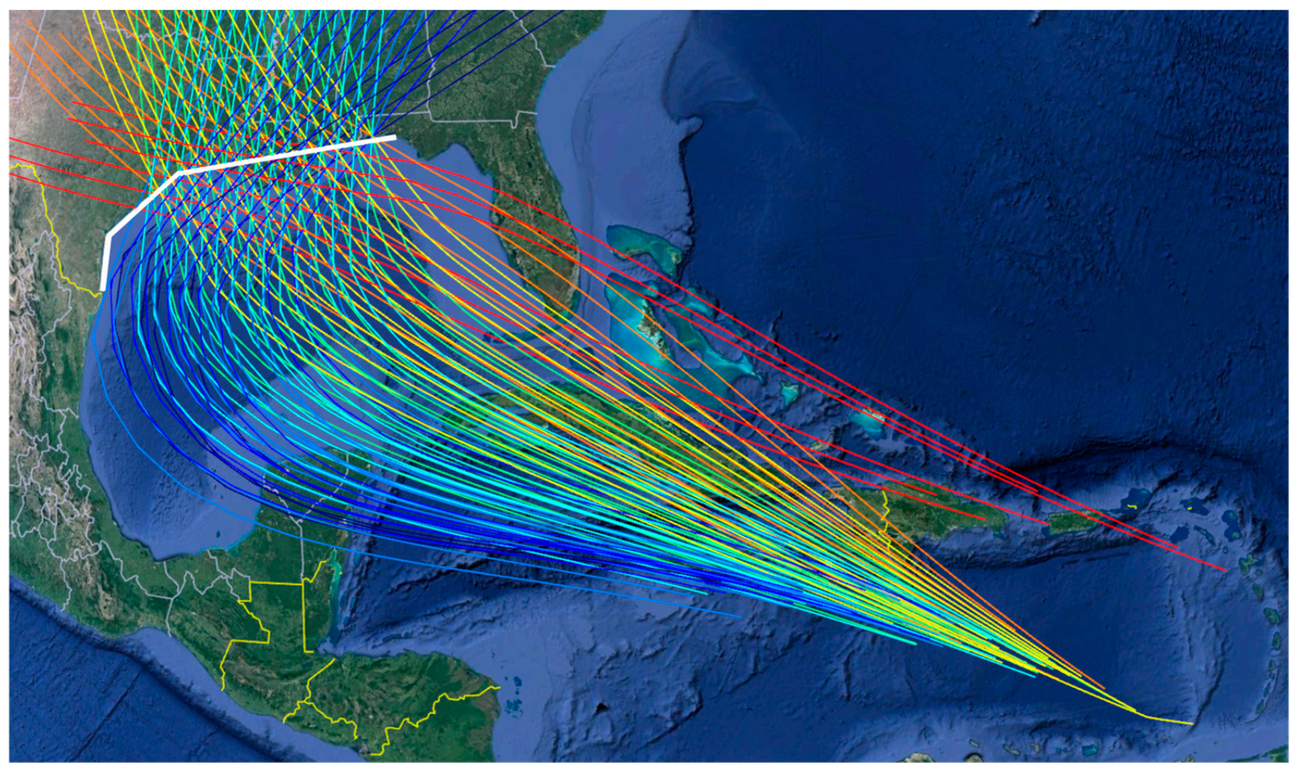
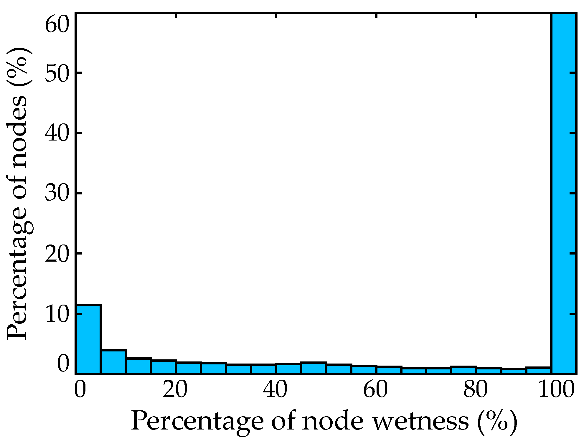
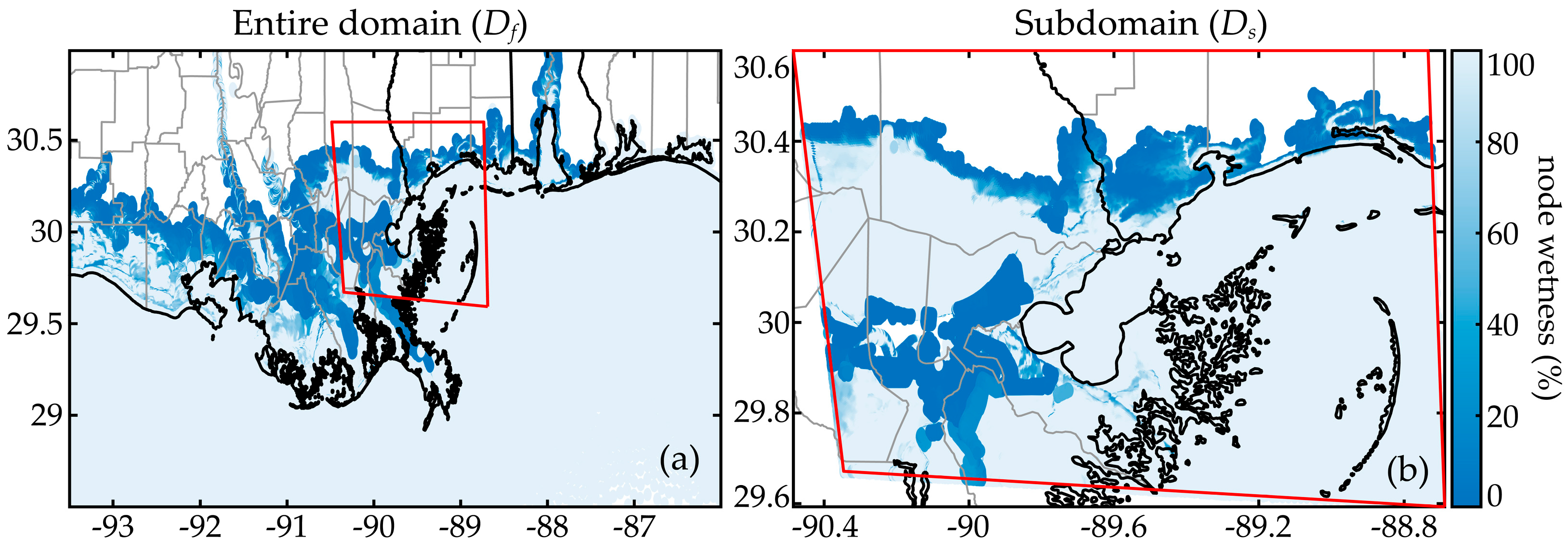
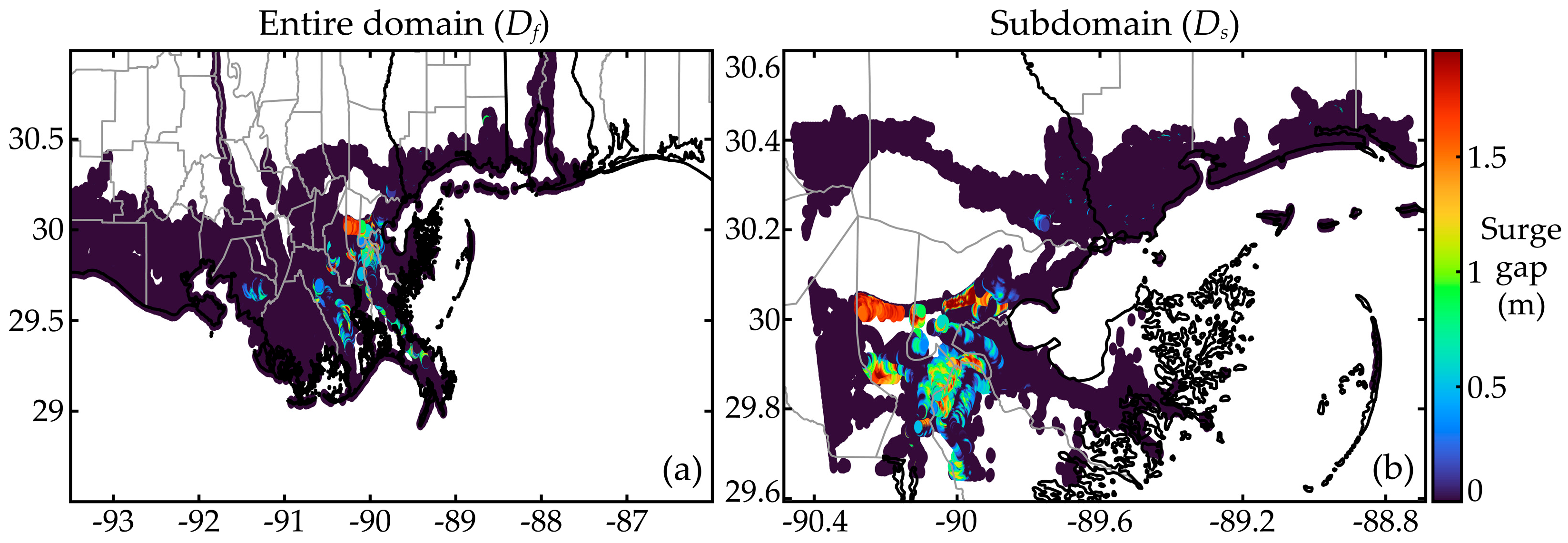

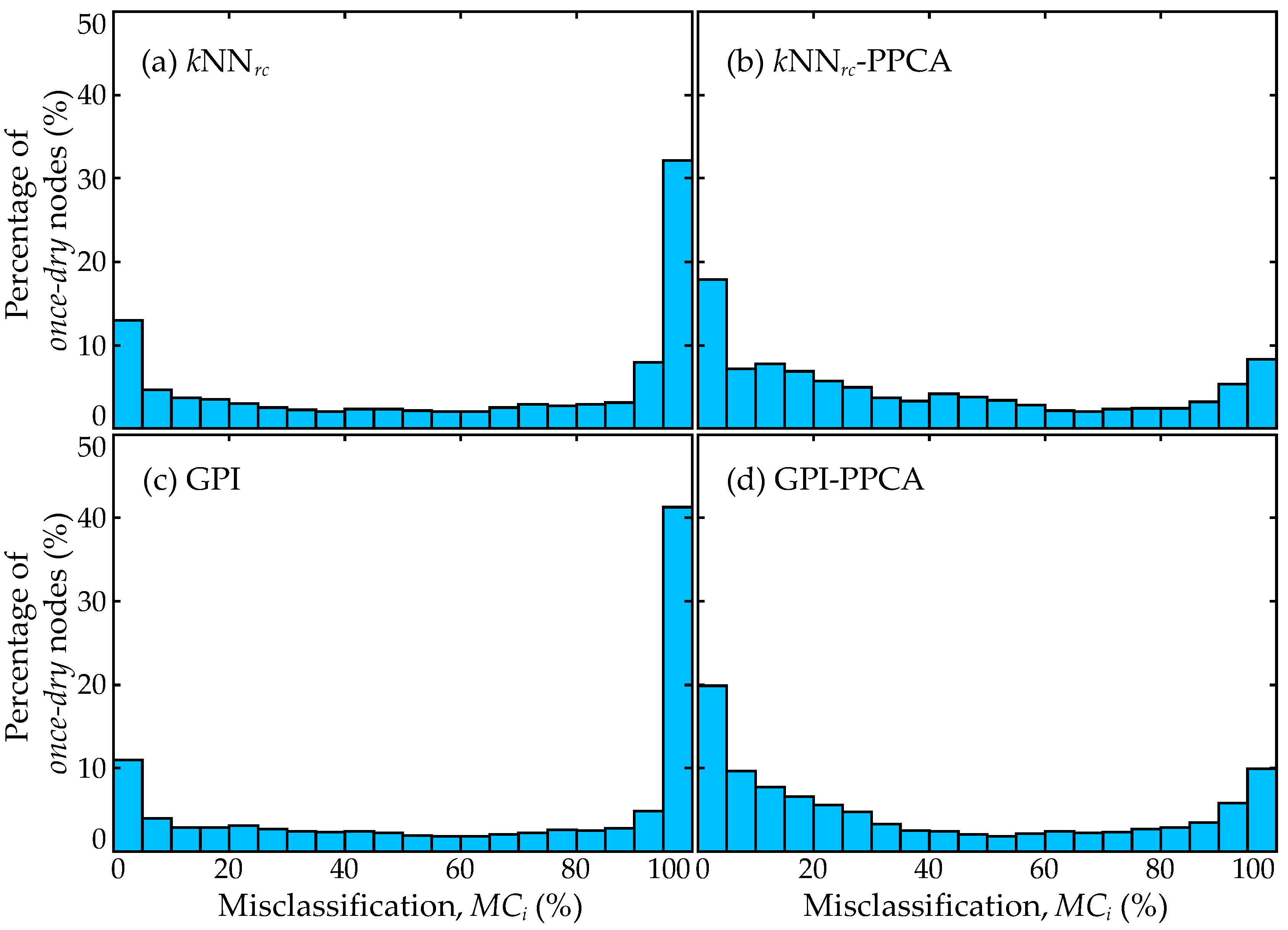
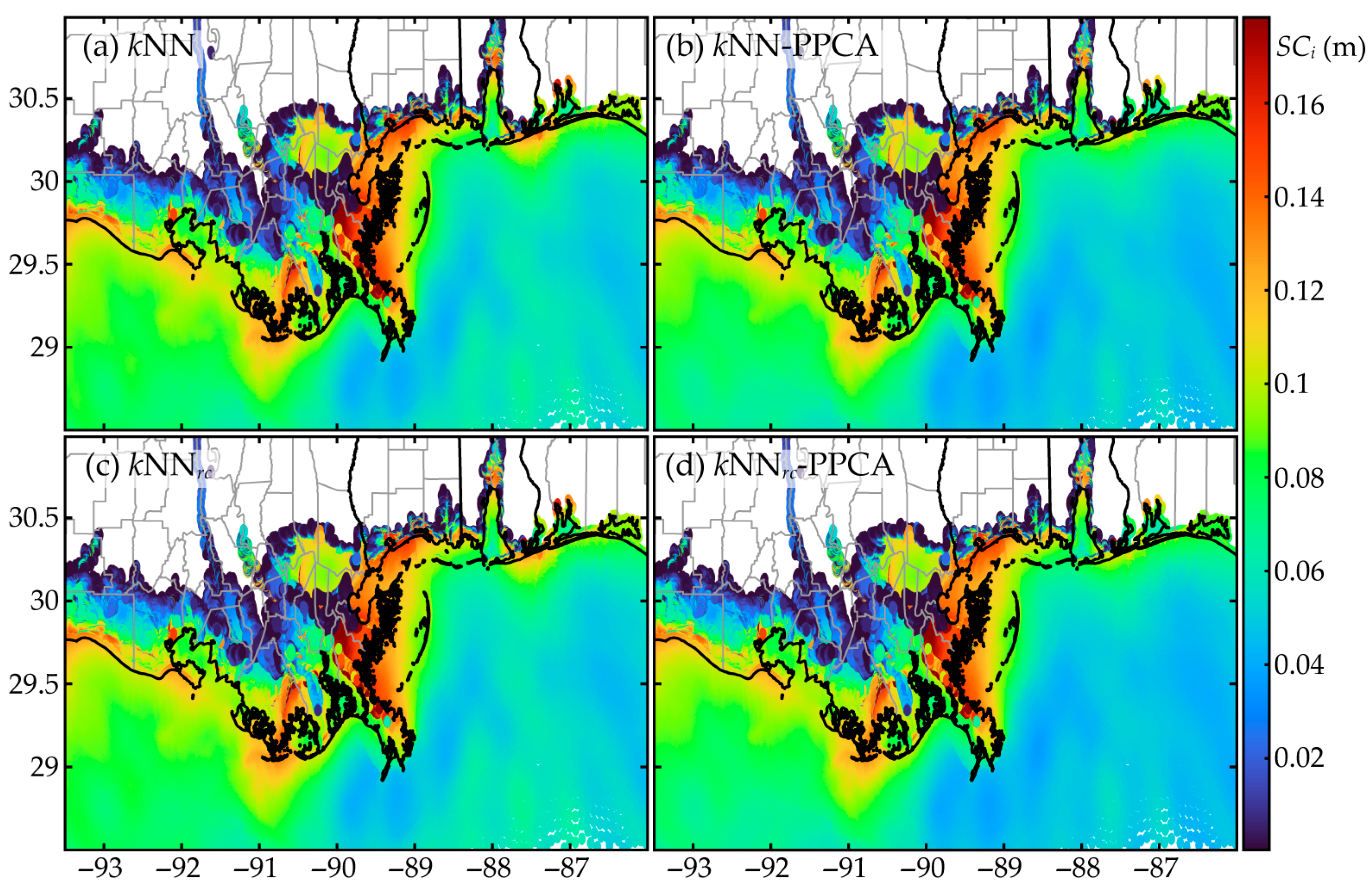
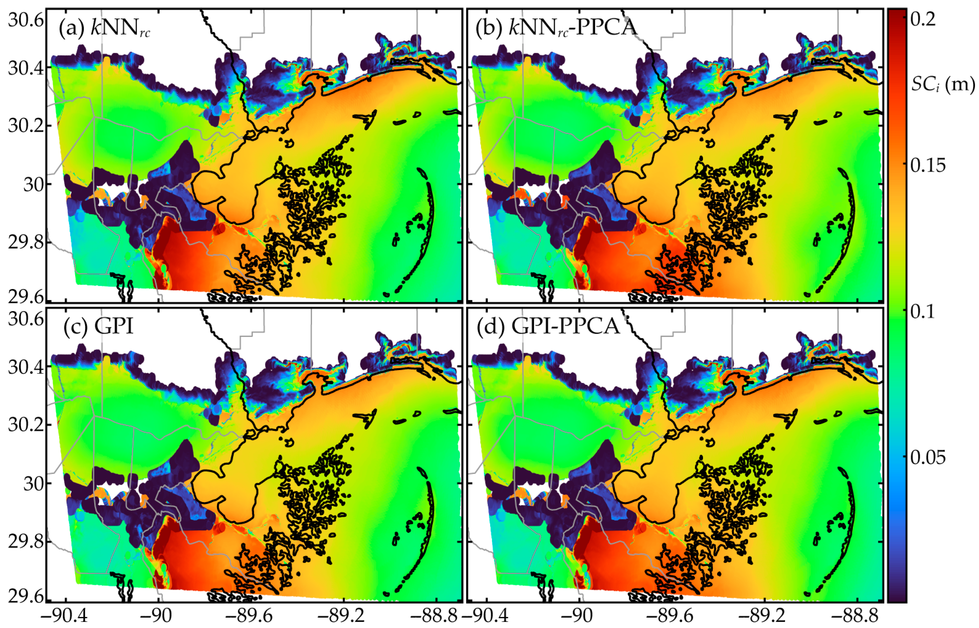
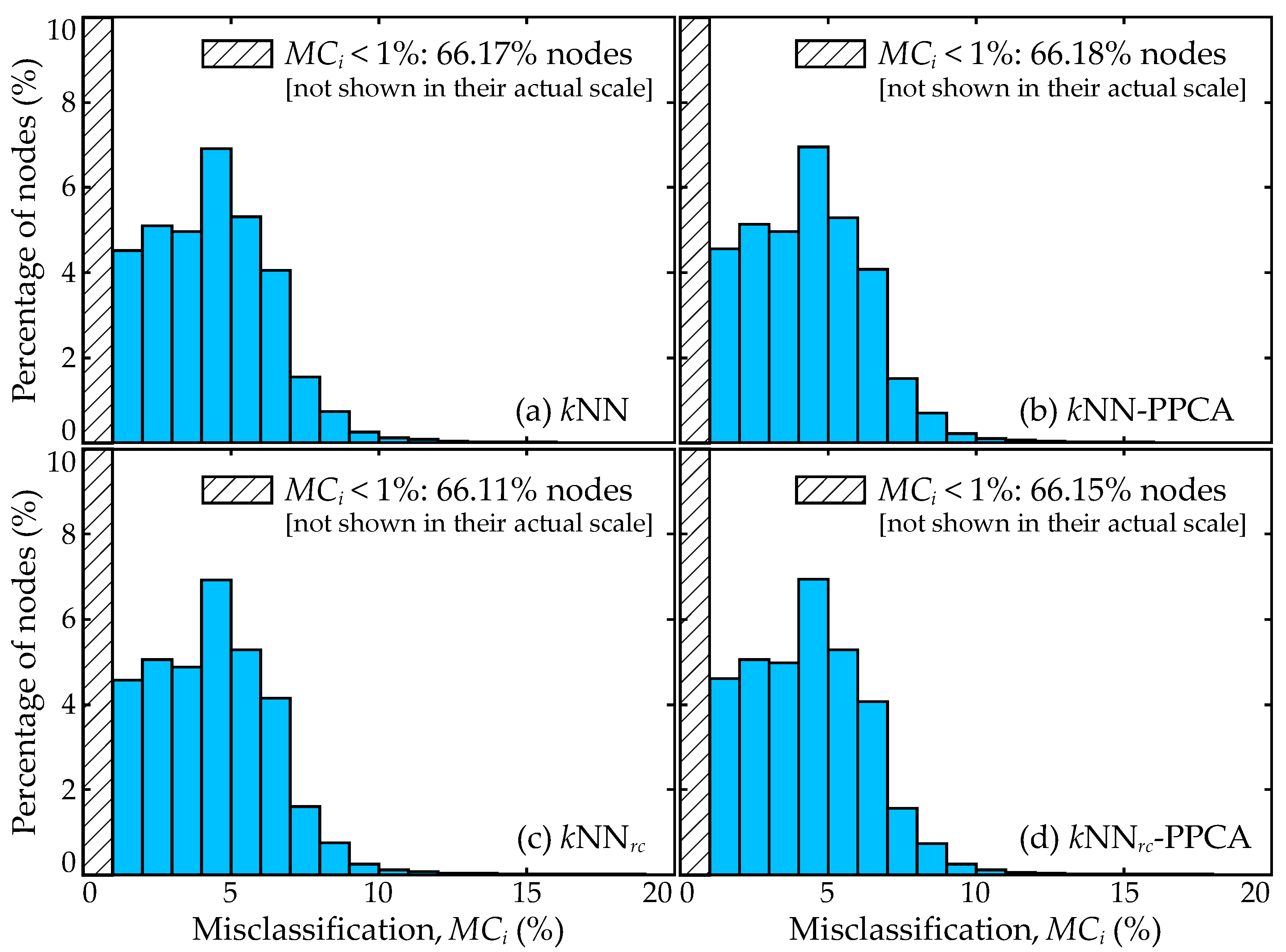
| ID | Storm Heading β (°) | Number of Different MTs (Landfall Locations) | Number of Storms per MT | Storm Parameter Range | ||
|---|---|---|---|---|---|---|
(mbar) | (km) | (m/s) | ||||
| 1 | −80 | 6 | 48 | [8 148] | [9.3 115.5] | [2.4 10.60] |
| 2 | −60 | 9 | 70 | [18 138] | [11.8 127.5] | [2.4 12.50] |
| 3 | −40 | 13 | 104 | [8 148] | [8.5 133.1] | [2.2 13.90] |
| 4 | −20 | 15 | 105 | [18 138] | [9.1 116.5] | [2.4 11.80] |
| 5 | 0 | 15 | 120 | [8 148] | [8.0 130.0] | [2.4 13.05] |
| 6 | 20 | 14 | 98 | [18 138] | [8.6 138.2] | [2.3 12.65] |
| 7 | 40 | 9 | 72 | [8 148] | [9.6 141.3] | [2.3 12.85] |
| 8 | 60 | 4 | 28 | [18 138] | [9.4 119.4] | [2.5 13.40] |
| Database | Statistics | Once-Dry | Surge Gap> (m) | ||||||
|---|---|---|---|---|---|---|---|---|---|
| 0.075 | 0.15 | 0.25 | 0.5 | 0.75 | 1 | 1.5 | |||
| Df | % of nodes | 41.40 | 21.77 | 13.91 | 8.86 | 3.77 | 1.86 | 0.99 | 0.35 |
| % inundated in database | 31.26 | 6.94 | 4.40 | 2.90 | 1.94 | 1.88 | 2.04 | 2.89 | |
| Ds | % of nodes | 39.73 | 37.18 | 27.67 | 20.26 | 10.59 | 5.99 | 3.55 | 1.28 |
| % inundated in database | 42.54 | 4.75 | 3.18 | 2.27 | 1.46 | 1.21 | 1.16 | 1.63 | |
| Database | Statistics | kNN | kNNrc | PPCA | GPI | ||||||||
|---|---|---|---|---|---|---|---|---|---|---|---|---|---|
| Df | % of nodes | 63.87 | 41.40 | 58.60 | 69.56 | 48.92 | 51.08 | 99.24 | 94.50 | 5.50 | N/A | ||
| % inundated in database | 33.35 | 25.75 | 35.15 | 32.09 | 24.93 | 37.31 | 31.17 | 29.16 | 67.30 | ||||
| Ds | % of nodes | 69.95 | 52.31 | 47.69 | 72.27 | 55.20 | 44.80 | 98.17 | 89.18 | 10.82 | 78.52 | 64.61 | 35.39 |
| % inundated in database | 26.40 | 15.07 | 44.08 | 26.37 | 15.97 | 44.84 | 28.78 | 25.15 | 59.82 | 55.51 | 55.18 | 55.10 | |
| Database | Statistics | kNN-PPCA | kNNrc-PPCA | GPI-PPCA | ||||||
|---|---|---|---|---|---|---|---|---|---|---|
| Df | % of nodes | 54.58 | 41.00 | 59.00 | 60.45 | 46.98 | 53.02 | N/A | ||
| % inundated in database | 33.34 | 26.81 | 34.34 | 32.13 | 26.23 | 35.70 | ||||
| Ds | % of nodes | 63.49 | 52.85 | 47.15 | 65.55 | 55.20 | 44.80 | 73.09 | 59.27 | 40.73 |
| % inundated in database | 24.49 | 16.77 | 42.50 | 25.08 | 17.74 | 42.66 | 55.55 | 55.10 | 55.23 | |
| Pseudo-Surge Database (Combination of Ss and Sc) | Corrected Pseudo-Surge Database (Ss Only) | ||||||||||
|---|---|---|---|---|---|---|---|---|---|---|---|
| kNN | kNNrc | PPCA | kNN-PPCA | kNNrc-PPCA | kNN | kNNrc | PPCA | kNN-PPCA | kNNrc-PPCA | ||
| All nodes | 7.69 | 7.69 | 7.79 | 7.51 | 7.53 | 7.85 | 7.87 | 8.10 | 7.69 | 7.73 | |
| Once-dry | 5.32 | 5.27 | 5.40 | 5.13 | 5.12 | 5.55 | 5.60 | 5.83 | 5.42 | 5.49 | |
| Surge gap> (m) | 0.25 | 2.27 | 2.18 | 2.11 | 2.17 | 2.10 | 2.88 | 3.13 | 2.94 | 2.79 | 3.05 |
| 0.5 | 1.85 | 1.75 | 1.74 | 1.81 | 1.72 | 2.52 | 2.91 | 2.59 | 2.44 | 2.83 | |
| 0.75 | 1.76 | 1.68 | 1.71 | 1.76 | 1.69 | 2.58 | 3.10 | 2.64 | 2.47 | 3.02 | |
| 1 | 1.89 | 1.81 | 1.86 | 1.90 | 1.84 | 2.90 | 3.47 | 2.93 | 2.77 | 3.35 | |
| 1.5 | 2.67 | 2.56 | 2.72 | 2.75 | 2.70 | 4.38 | 4.83 | 4.40 | 4.24 | 4.66 | |
| Node groups | 5.76 | 5.41 | 5.29 | 5.62 | 5.43 | 6.21 | 6.00 | 5.74 | 6.24 | 6.14 | |
| 5.00 | 5.13 | 7.29 | 4.79 | 4.85 | 5.08 | 5.22 | 7.45 | 4.86 | 4.92 | ||
| Pseudo-Surge Database (Combination of Ss and Sc) | Corrected Pseudo-Surge Database (Ss Only) | ||||||||||
|---|---|---|---|---|---|---|---|---|---|---|---|
| kNN | kNNrc | PPCA | kNN-PPCA | kNNrc-PPCA | kNN | kNNrc | PPCA | kNN-PPCA | kNNrc-PPCA | ||
| All nodes | 1.54 | 1.55 | 1.68 | 1.53 | 1.54 | 2.60 | 2.79 | 3.53 | 2.46 | 2.62 | |
| Once-dry | 3.57 | 3.57 | 3.90 | 3.54 | 3.55 | 6.14 | 6.58 | 8.38 | 5.79 | 6.18 | |
| Surge gap> (m) | 0.25 | 1.01 | 1.00 | 1.02 | 1.00 | 0.99 | 5.04 | 7.15 | 6.11 | 4.38 | 6.01 |
| 0.5 | 0.77 | 0.76 | 0.77 | 0.76 | 0.75 | 4.60 | 7.72 | 5.52 | 4.00 | 6.41 | |
| 0.75 | 0.69 | 0.68 | 0.69 | 0.69 | 0.68 | 4.55 | 8.53 | 5.24 | 4.00 | 7.03 | |
| 1 | 0.70 | 0.68 | 0.69 | 0.69 | 0.68 | 4.59 | 8.65 | 5.17 | 4.14 | 6.96 | |
| 1.5 | 0.86 | 0.84 | 0.84 | 0.86 | 0.84 | 5.24 | 7.96 | 6.32 | 5.25 | 6.63 | |
| Node groups | 3.63 | 3.67 | 4.03 | 3.72 | 3.75 | 8.37 | 8.86 | 8.69 | 7.83 | 8.38 | |
| 3.52 | 3.47 | 1.67 | 3.42 | 3.37 | 4.56 | 4.39 | 2.94 | 4.38 | 4.24 | ||
| Pseudo-Surge Database (Combination of Ss and Sc) | Corrected Pseudo-Surge Database (Ss Only) | ||||||||||
|---|---|---|---|---|---|---|---|---|---|---|---|
| kNN | kNNrc | PPCA | kNN-PPCA | kNNrc-PPCA | kNN | kNNrc | PPCA | kNN-PPCA | kNNrc-PPCA | ||
| All nodes | 0.68 | 0.67 | 0.62 | 0.66 | 0.66 | 1.82 | 2.05 | 2.90 | 1.68 | 1.89 | |
| Once-dry | 1.63 | 1.61 | 1.50 | 1.60 | 1.59 | 4.39 | 4.94 | 7.01 | 4.07 | 4.56 | |
| Surge gap> (m) | 0.25 | 0.31 | 0.30 | 0.32 | 0.30 | 0.30 | 4.82 | 7.00 | 6.02 | 4.15 | 5.84 |
| 0.5 | 0.21 | 0.20 | 0.21 | 0.21 | 0.20 | 4.41 | 7.60 | 5.43 | 3.81 | 6.29 | |
| 0.75 | 0.19 | 0.18 | 0.19 | 0.19 | 0.18 | 4.38 | 8.42 | 5.15 | 3.83 | 6.91 | |
| 1 | 0.22 | 0.20 | 0.20 | 0.22 | 0.20 | 4.43 | 8.52 | 5.06 | 3.99 | 6.82 | |
| 1.5 | 0.34 | 0.28 | 0.28 | 0.34 | 0.28 | 5.12 | 7.85 | 6.22 | 5.13 | 6.48 | |
| Node groups | 1.36 | 1.39 | 1.52 | 1.37 | 1.40 | 7.22 | 7.78 | 7.34 | 6.69 | 7.28 | |
| 1.83 | 1.82 | 1.12 | 1.76 | 1.75 | 2.40 | 2.23 | 1.24 | 2.24 | 2.15 | ||
| Pseudo-Surge Database (Combination of Ss and Sc) | Corrected Pseudo-Surge Database (Ss Only) | ||||||||||
|---|---|---|---|---|---|---|---|---|---|---|---|
| kNN | kNNrc | PPCA | kNN-PPCA | kNNrc-PPCA | kNN | kNNrc | PPCA | kNN-PPCA | kNNrc-PPCA | ||
| All nodes | 0.86 | 0.88 | 1.06 | 0.87 | 0.88 | 0.78 | 0.74 | 0.63 | 0.78 | 0.73 | |
| Once-dry | 1.93 | 1.96 | 2.41 | 1.94 | 1.97 | 1.74 | 1.63 | 1.37 | 1.73 | 1.62 | |
| Surge gap> (m) | 0.25 | 0.70 | 0.70 | 0.70 | 0.70 | 0.69 | 0.22 | 0.15 | 0.09 | 0.24 | 0.16 |
| 0.5 | 0.55 | 0.55 | 0.56 | 0.55 | 0.55 | 0.19 | 0.12 | 0.08 | 0.19 | 0.13 | |
| 0.75 | 0.50 | 0.50 | 0.50 | 0.49 | 0.50 | 0.17 | 0.11 | 0.09 | 0.17 | 0.12 | |
| 1 | 0.47 | 0.49 | 0.49 | 0.47 | 0.49 | 0.16 | 0.12 | 0.11 | 0.15 | 0.14 | |
| 1.5 | 0.52 | 0.56 | 0.56 | 0.52 | 0.56 | 0.12 | 0.11 | 0.10 | 0.12 | 0.14 | |
| Node groups | 2.27 | 2.28 | 2.51 | 2.34 | 2.35 | 1.15 | 1.09 | 1.35 | 1.14 | 1.09 | |
| 1.69 | 1.66 | 0.54 | 1.67 | 1.62 | 2.16 | 2.15 | 1.71 | 2.13 | 2.09 | ||
| Pseudo-Surge Database (Combination of Ss and Sc) | Corrected Pseudo-Surge Database (Ss Only) | ||||||||||||||
|---|---|---|---|---|---|---|---|---|---|---|---|---|---|---|---|
| kNN | kNNrc | GPI | PPCA | kNN-PPCA | kNNrc-PPCA | GPI-PPCA | kNN | kNNrc | GPI | PPCA | kNN-PPCA | kNNrc-PPCA | GPI-PPCA | ||
| All nodes | 9.26 | 9.25 | 9.13 | 9.63 | 9.39 | 9.40 | 9.20 | 9.61 | 9.67 | 10.72 | 10.08 | 9.58 | 9.83 | 9.91 | |
| Once-dry | 5.91 | 5.82 | 5.85 | 6.06 | 5.77 | 5.69 | 5.64 | 6.48 | 6.62 | 7.29 | 6.78 | 6.25 | 6.52 | 7.43 | |
| Surge gap> (m) | 0.25 | 1.98 | 1.86 | 1.86 | 1.84 | 1.92 | 1.81 | 1.84 | 2.73 | 3.34 | 2.82 | 2.70 | 2.60 | 3.24 | 3.92 |
| 0.5 | 1.58 | 1.46 | 1.47 | 1.47 | 1.55 | 1.46 | 1.49 | 2.31 | 3.06 | 2.35 | 2.28 | 2.20 | 2.97 | 3.37 | |
| 0.75 | 1.36 | 1.29 | 1.30 | 1.32 | 1.36 | 1.30 | 1.33 | 2.11 | 2.97 | 2.15 | 2.09 | 2.01 | 2.91 | 3.11 | |
| 1 | 1.35 | 1.28 | 1.29 | 1.33 | 1.35 | 1.31 | 1.34 | 2.13 | 2.93 | 2.22 | 2.15 | 2.03 | 2.86 | 3.17 | |
| 1.5 | 1.98 | 1.87 | 1.89 | 1.99 | 2.03 | 1.98 | 2.01 | 3.15 | 3.61 | 3.40 | 3.29 | 3.12 | 3.57 | 5.09 | |
| Node groups | 5.01 | 4.99 | 5.62 | 6.00 | 4.95 | 4.94 | 5.22 | 5.91 | 6.30 | 6.70 | 6.81 | 5.95 | 6.41 | 8.22 | |
| 6.90 | 6.84 | 6.38 | 6.48 | 6.56 | 6.52 | 6.26 | 7.09 | 7.02 | 8.37 | 6.57 | 6.53 | 6.64 | 6.27 | ||
| Pseudo-Surge Database (Combination of Ss and Sc) | Corrected Pseudo-Surge Database (Ss Only) | ||||||||||||||
|---|---|---|---|---|---|---|---|---|---|---|---|---|---|---|---|
| kNN | kNNrc | GPI | PPCA | kNN-PPCA | kNNrc-PPCA | GPI-PPCA | kNN | kNNrc | GPI | PPCA | kNN-PPCA | kNNrc-PPCA | GPI-PPCA | ||
| All nodes | 1.13 | 1.13 | 1.15 | 1.21 | 1.12 | 1.13 | 1.14 | 2.37 | 2.97 | 3.78 | 3.35 | 2.21 | 2.78 | 4.40 | |
| Once-dry | 2.78 | 2.76 | 2.80 | 2.96 | 2.75 | 2.74 | 2.79 | 5.90 | 7.40 | 9.40 | 8.34 | 5.49 | 6.90 | 11.00 | |
| Surge gap> (m) | 0.25 | 0.78 | 0.78 | 0.77 | 0.78 | 0.78 | 0.77 | 0.78 | 5.47 | 10.37 | 4.83 | 5.03 | 4.80 | 9.21 | 11.19 |
| 0.5 | 0.60 | 0.59 | 0.59 | 0.59 | 0.60 | 0.59 | 0.59 | 5.21 | 11.11 | 4.03 | 4.38 | 4.53 | 9.93 | 10.33 | |
| 0.75 | 0.51 | 0.51 | 0.51 | 0.51 | 0.51 | 0.51 | 0.51 | 5.02 | 11.51 | 3.55 | 3.99 | 4.40 | 10.43 | 9.81 | |
| 1 | 0.51 | 0.51 | 0.51 | 0.51 | 0.51 | 0.50 | 0.51 | 4.83 | 10.80 | 3.61 | 4.11 | 4.41 | 9.57 | 9.94 | |
| 1.5 | 0.67 | 0.65 | 0.66 | 0.65 | 0.66 | 0.65 | 0.66 | 5.20 | 8.41 | 4.77 | 5.48 | 5.28 | 6.92 | 13.74 | |
| Node groups | 2.15 | 2.25 | 2.63 | 3.21 | 2.22 | 2.29 | 2.70 | 7.46 | 10.20 | 9.00 | 9.33 | 7.23 | 9.77 | 16.27 | |
| 3.47 | 3.38 | 3.11 | 1.28 | 3.26 | 3.23 | 2.92 | 4.18 | 3.95 | 10.15 | 1.90 | 3.81 | 3.74 | 3.32 | ||
| Pseudo-Surge Database (Combination of Ss and Sc) | Corrected Pseudo-Surge Database (Ss Only) | ||||||||||||||
|---|---|---|---|---|---|---|---|---|---|---|---|---|---|---|---|
| kNN | kNNrc | GPI | PPCA | kNN-PPCA | kNNrc-PPCA | GPI-PPCA | kNN | kNNrc | GPI | PPCA | kNN-PPCA | kNNrc-PPCA | GPI-PPCA | ||
| All nodes | 0.50 | 0.50 | 0.49 | 0.51 | 0.49 | 0.50 | 0.48 | 1.82 | 2.47 | 3.49 | 3.07 | 1.68 | 2.28 | 3.97 | |
| Once-dry | 1.26 | 1.26 | 1.22 | 1.28 | 1.25 | 1.25 | 1.22 | 4.57 | 6.22 | 8.77 | 7.72 | 4.23 | 5.75 | 10.00 | |
| Surge gap> (m) | 0.25 | 0.23 | 0.23 | 0.23 | 0.24 | 0.23 | 0.23 | 0.24 | 5.19 | 10.19 | 4.62 | 4.87 | 4.54 | 9.04 | 11.07 |
| 0.5 | 0.17 | 0.16 | 0.16 | 0.16 | 0.17 | 0.16 | 0.16 | 4.98 | 10.95 | 3.84 | 4.23 | 4.30 | 9.79 | 10.23 | |
| 0.75 | 0.14 | 0.13 | 0.14 | 0.13 | 0.14 | 0.13 | 0.14 | 4.83 | 11.37 | 3.37 | 3.84 | 4.21 | 10.29 | 9.71 | |
| 1 | 0.14 | 0.14 | 0.14 | 0.14 | 0.14 | 0.14 | 0.14 | 4.65 | 10.65 | 3.45 | 3.97 | 4.22 | 9.43 | 9.85 | |
| 1.5 | 0.22 | 0.20 | 0.21 | 0.20 | 0.21 | 0.20 | 0.20 | 5.05 | 8.27 | 4.63 | 5.35 | 5.13 | 6.78 | 13.66 | |
| Node groups | 0.76 | 0.84 | 1.06 | 1.34 | 0.78 | 0.85 | 1.05 | 6.79 | 9.60 | 8.39 | 8.74 | 6.58 | 9.21 | 15.77 | |
| 1.80 | 1.79 | 1.52 | 0.87 | 1.69 | 1.69 | 1.46 | 2.13 | 2.06 | 9.48 | 1.02 | 1.96 | 1.94 | 1.60 | ||
| Pseudo-Surge Database (Combination of Ss and Sc) | Corrected Pseudo-Surge Database (Ss Only) | ||||||||||||||
|---|---|---|---|---|---|---|---|---|---|---|---|---|---|---|---|
| kNN | kNNrc | GPI | PPCA | kNN-PPCA | kNNrc-PPCA | GPI-PPCA | kNN | kNNrc | GPI | PPCA | kNN-PPCA | kNNrc-PPCA | GPI-PPCA | ||
| All nodes | 0.63 | 0.63 | 0.66 | 0.70 | 0.63 | 0.63 | 0.66 | 0.56 | 0.50 | 0.30 | 0.28 | 0.53 | 0.49 | 0.43 | |
| Once-dry | 1.52 | 1.50 | 1.58 | 1.50 | 1.50 | 1.49 | 1.57 | 1.32 | 1.18 | 0.63 | 0.62 | 1.26 | 1.15 | 1.00 | |
| Surge gap> (m) | 0.25 | 0.55 | 0.54 | 0.54 | 0.54 | 0.54 | 0.54 | 0.54 | 0.28 | 0.19 | 0.20 | 0.16 | 0.26 | 0.17 | 0.12 |
| 0.5 | 0.43 | 0.43 | 0.43 | 0.43 | 0.43 | 0.43 | 0.43 | 0.23 | 0.16 | 0.19 | 0.16 | 0.22 | 0.14 | 0.11 | |
| 0.75 | 0.38 | 0.38 | 0.38 | 0.38 | 0.38 | 0.37 | 0.38 | 0.20 | 0.14 | 0.18 | 0.15 | 0.19 | 0.14 | 0.10 | |
| 1 | 0.37 | 0.37 | 0.37 | 0.37 | 0.37 | 0.36 | 0.37 | 0.18 | 0.14 | 0.17 | 0.14 | 0.18 | 0.14 | 0.10 | |
| 1.5 | 0.45 | 0.45 | 0.45 | 0.45 | 0.45 | 0.45 | 0.45 | 0.15 | 0.14 | 0.14 | 0.12 | 0.16 | 0.14 | 0.09 | |
| Node groups | 1.38 | 1.42 | 1.57 | 1.87 | 1.44 | 1.44 | 1.64 | 0.67 | 0.60 | 0.61 | 0.59 | 0.64 | 0.57 | 0.51 | |
| 1.67 | 1.59 | 1.58 | 0.41 | 1.57 | 1.54 | 1.45 | 2.05 | 1.89 | 0.67 | 0.88 | 1.85 | 1.79 | 1.72 | ||
Disclaimer/Publisher’s Note: The statements, opinions and data contained in all publications are solely those of the individual author(s) and contributor(s) and not of MDPI and/or the editor(s). MDPI and/or the editor(s) disclaim responsibility for any injury to people or property resulting from any ideas, methods, instructions or products referred to in the content. |
© 2025 by the authors. Licensee MDPI, Basel, Switzerland. This article is an open access article distributed under the terms and conditions of the Creative Commons Attribution (CC BY) license (https://creativecommons.org/licenses/by/4.0/).
Share and Cite
Jung, W.; Irwin, C.; Taflanidis, A.A.; Nadal-Caraballo, N.C.; Aucoin, L.A.; Yawn, M.C. Advances in Imputation Strategies Supporting Peak Storm Surge Surrogate Modeling. J. Mar. Sci. Eng. 2025, 13, 1678. https://doi.org/10.3390/jmse13091678
Jung W, Irwin C, Taflanidis AA, Nadal-Caraballo NC, Aucoin LA, Yawn MC. Advances in Imputation Strategies Supporting Peak Storm Surge Surrogate Modeling. Journal of Marine Science and Engineering. 2025; 13(9):1678. https://doi.org/10.3390/jmse13091678
Chicago/Turabian StyleJung, WoongHee, Christopher Irwin, Alexandros A. Taflanidis, Norberto C. Nadal-Caraballo, Luke A. Aucoin, and Madison C. Yawn. 2025. "Advances in Imputation Strategies Supporting Peak Storm Surge Surrogate Modeling" Journal of Marine Science and Engineering 13, no. 9: 1678. https://doi.org/10.3390/jmse13091678
APA StyleJung, W., Irwin, C., Taflanidis, A. A., Nadal-Caraballo, N. C., Aucoin, L. A., & Yawn, M. C. (2025). Advances in Imputation Strategies Supporting Peak Storm Surge Surrogate Modeling. Journal of Marine Science and Engineering, 13(9), 1678. https://doi.org/10.3390/jmse13091678


