Abstract
This study proposes a hybrid sea level prediction model by coupling a dynamically optimized variational mode decomposition (VMD) with a convolutional bidirectional gated recurrent unit (CNN-BiGRU). The VMD decomposition is fine-tuned using the grey wolf optimizer and evaluated via entropy criteria to minimize mode mixing. The resulting components are processed by CNN-BiGRU to capture spatial features and temporal dependencies, and predictions are reconstructed from the integrated outputs. Validated on monthly sea level data from Kanmen and Zhapo stations, the model achieves high accuracy with an RMSE of 13.857 mm and 16.230 mm, MAE of 10.659 mm and 13.129 mm, and NSE of 0.986 and 0.980. With a 6-month time step, the proposed strategy effectively captures both periodic and trend signals, demonstrating strong dynamic tracking and error convergence. It significantly improves prediction accuracy and provides reliable support for storm surge warning and coastal management.
1. Introduction
Global warming has resulted in a persistent rise in sea level, which represents one of the most critical global environmental challenges. This phenomenon is primarily driven by the accelerated melting of glaciers and the thermal expansion of seawater. Over the past five decades, global mean sea level has exhibited a clear accelerating trend [1,2]. According to a 2024 report by the National Aeronautics and Space Administration (NASA), the global sea level increased by 0.59 cm in 2024 compared with 2023, amounting to a cumulative rise of approximately 10.5 cm over the 31-year satellite observation record [3]. The continuous rise in sea level has intensified coastal hazards such as shoreline erosion, seawater intrusion, and saltwater upwelling [4,5], posing direct threats to coastal infrastructure, agricultural ecosystems, and the livelihoods of urban populations in low-lying coastal regions.
China, as a major coastal nation characterized by extensive shorelines and densely populated, economically vital cities, is highly susceptible to the impacts of sea level rise. From 1980 to 2024, the average annual rate of sea level increase along China’s coast was approximately 3.5 mm yr−1, about 20% higher than the global mean rate [6]. The most pronounced increases have occurred in northern marine regions, particularly in the Bohai Sea and the Yellow Sea [7]. In contrast, coastal cities in southern China frequently experience severe urban waterlogging and seawater intrusion. These variations are primarily driven by astronomical tides and extreme meteorological events, such as Typhoon Matmo and Typhoon Hagibis [8,9]. Such events highlight the inherent limitations of static, large-scale sea level prediction approaches in capturing the dynamic and evolving nature of marine hazards. Sea level rise has thus transitioned from a projected future risk to a pressing contemporary hazard.
Accurate prediction of future sea level variations is essential for climate adaptation, coastal zone planning, and flood risk management. Nevertheless, existing prediction methods exhibit notable limitations in stability, generalization capability, and responsiveness to extreme events, which impede their capacity to accurately capture the nonlinear and accelerating trend of sea level rise. For a detailed overview of existing sea level prediction methods, readers are referred to Section 2: Related Work. Accordingly, the development of high-precision sea level prediction models has emerged as a critical global research priority, aimed at providing indispensable scientific support for climate adaptation, coastal planning, and flood risk management.
Therefore, this paper proposes a strategy of integrating adaptive decomposition and deep learning to address the challenges of non-stationarity and complexity in sea level prediction. This approach optimizes key parameters by combining entropy criteria with the GWO algorithm to adapt to the non-stationary characteristics of sea level time series, followed by prediction using a CNN-BiGRU model for decomposed signals. The primary contributions of our proposed prediction strategy can be described as follows:
- (1)
- The GWO algorithm, combined with four entropy criteria including envelope entropy (EnVeEn), fuzzy entropy (FuzzyEn), permutation entropy (PeEn), and sample entropy (SpEn), can achieve dynamic optimization of VMD parameters such as the number of modes K and penalty factor α, resolving the mode aliasing problem induced by traditional empirical settings.
- (2)
- Intrinsic modal components generated by optimized VMD decomposition are input into a convolutional neural network-bidirectional gated recurrent unit (CNN-BiGRU) coupled model. In this model, spatially relevant features are extracted by the CNN layer. Long- and short-term dependencies in the time series are captured by the BiGRU layer through learning.
- (3)
- Comparative analysis of time feature length windows and statistical analysis of monthly-scale prediction performance help to improve model adaptability to different time scales and verify the accuracy and stability of prediction results.
- (4)
- Site-specific discrepancies in regional sea level predictions are identified and, through a “phenomenon–cause–scientific significance” framework, translated into actionable insights for climate adaptation, coastal planning, and storm surge and flood risk management.
The detailed structure of this article is as follows. Section 2 provides an overview of existing sea level prediction methods. Section 3 introduces the proposed sea level prediction framework and its detailed implementation process. Section 4 presents experimental results analyzed from multiple perspectives. Section 5 further evaluates the performance of the proposed method through feature time step analysis, monthly statistical feature evaluation, and assessments of generalizability across multiple datasets, while providing insights into site-specific predictions and regional dynamic insights. Finally, the conclusions are illustrated in Section 6.
2. Related Work
2.1. Signal Decomposition Methods
Obvious nonlinear, non-stationary, and multivariate characteristics are exhibited by sea level changes, making it difficult for traditional time series prediction methods to achieve ideal results. To address this issue, attempts have been made in numerous studies to decompose the original signal, aiming to reduce its non-stationarity and enhance prediction accuracy. Methods such as empirical mode decomposition (EMD) [10], complete ensemble empirical mode decomposition with adaptive noise (CEEMDAN) [11], wavelet transform (WT) [12], and singular spectrum analysis (SSA) [13] are widely applied in studies on sea level changes. However, some shortcomings of these methods have been exposed in practical applications. For instance, the mode mixing phenomenon is exhibited by EMD. Improvements are still needed for CEEMDAN in terms of computational efficiency and details of noise processing. The decomposition quality is affected by the boundary effect of WT. The decomposition performance of SSA is highly dependent on window length selection. In contrast, variational mode decomposition (VMD) is an adaptive signal decomposition method based on the variational principle, which can effectively overcome some of the shortcomings mentioned above [14]. Complex sea level signals are decomposed by VMD into multiple Intrinsic Mode Functions (IMFs) with different center frequencies, with the decomposition process exhibiting good noise resistance and modal integrity [15].
Although certain advantages of VMD have been demonstrated in processing non-stationary signals, significant impacts on prediction performance are exerted by its parameter settings (such as the number of modes K and penalty factor α). Different decomposition results may be induced by varying parameter combinations, thereby affecting the accuracy of subsequent prediction models. To address this issue, the selection of suitable fitness functions and the application of intelligent optimization algorithms can be employed to determine the optimal parameters of VMD, with examples including genetic algorithm (GA) [16], particle swarm optimization (PSO) [17], and grey wolf optimization (GWO) [18,19,20], and the Greylag Goose Optimization (GGO) [21], and the Modified Al-Biruni Earth Radius (MBER) [22].
2.2. Machine Learning Methods
To effectively enhance the accuracy of sea level prediction, several machine learning methods, including support vector machine (SVM) [23], random forest (RF) [24], and extreme gradient boosting (XGBoost) [25], have been employed for predicting signal features. However, conventional machine learning approaches exhibit limitations in processing high-dimensional and complex time series data, including limited generalization capabilities and challenges in capturing long-term dependencies [26]. For instance, the sensitivity of SVM to the selection of kernel functions has been observed. RF is prone to overfitting, with weak extrapolation ability for long-term trends noted. Insufficient capture of extreme events by XGBoost may easily result in model bias.
2.3. Deep Learning Methods
In recent years, deep learning has been widely applied in the field of ocean time-series data analysis. Long short-term memory networks (LSTM) and their variants, gated recurrent units (GRU), are capable of effectively capturing long-term dependency information in time series [27,28,29,30]. The modeling ability of complex sequences is further enhanced by Bidirectional LSTM (BiLSTM) through the simultaneous consideration of both forward and backward time series information [31]. Single deep learning models, although powerful in feature extraction, still struggle to achieve satisfactory prediction accuracy when handling highly complex and uncertain sea level variation signals. They are prone to falling into local optima and often fail to fully capture the nonlinear and dynamic characteristics of sea level changes.
This has motivated the development of hybrid architectures that leverage complementary model strengths to enhance prediction accuracy. Such frameworks have shown promising results in sea level prediction. For example, several hybrid models have been proposed, including a CNN-BiGRU model optimized via Bayesian Optimization (BO-CNN-BiGRU) [32], an Ensemble Empirical Mode Decomposition combined with LSTM (EEMD–LSTM) [33], a VMD-LSTM [34], a VMD-CNN-BiLSTM [15], and a hybrid scheme integrating Empirical Mode Decomposition with a Radial Basis Function Neural Network optimized using Particle Swarm Optimization (EMD-PSO-RBFNN) [35].
2.4. General Remarks
Despite the enhanced performance of these hybrid frameworks, they continue to face challenges in accurately capturing the complex, nonlinear, and region-specific dynamics of sea level change. In particular, the selection of fitness functions during signal decomposition and the application of intelligent optimization algorithms remain insufficiently explored and lack systematic investigation. These limitations highlight the need for the development of novel hybrid strategies that can robustly simulate regional sea level dynamics while ensuring generalization across diverse coastal environments.
To address these limitations, this study proposes an innovative framework for coastal sea level prediction based on Dynamically Tuned Variational Mode Decomposition (VMD) and a Convolutional Bidirectional Gated Recurrent Unit (CNN-BiGRU) model. This approach adaptively determines the optimal decomposition parameters for sea level signals by dynamically tuning the K and α parameters of VMD using the GWO algorithm in combination with entropy-based criteria, thereby accommodating the non-stationary characteristics of sea level time series. The decomposed signals are subsequently processed by a CNN-BiGRU model, enhancing feature recognition and substantially improving the accuracy of subsequent sea level predictions.
3. Materials and Methods
3.1. Overall Framework
In order to address the impact of nonlinearity and non-stationarity on sea level prediction, this paper considers the characteristics of sea level time-series data from the perspective of parameter adaptive optimization and deep learning fusion. The proposed prediction scheme is illustrated in Figure 1. The main components of our strategy are as follows: (1) Dynamic tuning of variational mode decomposition (VMD) parameters based on grey wolf optimization (GWO); (2) Local spatiotemporal feature extraction via convolutional neural networks (CNN); (3) Bidirectional long-term temporal dependency modeling with bidirectional gated recurrent unit (BiGRU). The performance of the prediction scheme is evaluated from subjective prediction quality and prediction error indicators.
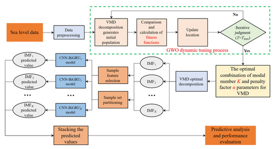
Figure 1.
Flow chart for predicting sea level changes via the synergistic integration of optimal signal decomposition and deep learning.
3.2. Variational Mode Decomposition and Its Dynamic Optimization
3.2.1. Variational Mode Decomposition Theory
Sea level changes are influenced by multiple factors such as global climate trends, regional hydrological dynamics, seasonal fluctuations, and short-term extreme events. Direct input into prediction models is likely to result in feature confusion and accuracy loss since the underlying signals exhibit changes in nonlinear and non-stationary characteristics [36]. Using an adaptive decomposition mechanism, the variational mode decomposition (VMD) method divides down the initial sea level sequence into several Intrinsic Mode Functions (IMFs) with distinct center frequencies. The constraint structure is expressed as follows:
where represents the partial derivative of time t. is the Dirac delta function. . represents a convolution operation. is the L2-norm (Euclidean Norm). K is the number of decomposed modes, and and are the k-th mode component and center frequency after decomposition, respectively. is the initial signal. The goal is to minimize the sum of the bandwidths of each component and ensure that the sum of the components is equal to the original signal.
After that, the Lagrange multiplier and penalty factor α are added to make the issue unconstrained. Alternating direction method of multipliers (ADMM) is employed to iteratively update the components, central frequencies, and Lagrange multipliers until convergence is attained.
Among these, the adequacy and redundancy of the decomposition are determined by K [37]. Under-decomposition is caused by an insufficient K value, while over-decomposition is induced by an excessive K value. The modal bandwidth is controlled by the penalty factor α [14]. Inadequate dispersion of the frequency distribution is brought about by an excessively small α, whereas loss of details due to excessive compression is caused by an overly large α. These two parameters are core factors influencing decomposition quality and must be determined through dynamic parameter tuning to enhance the quality of the decomposition process.
3.2.2. Dynamic Tuning Process
Characteristics of sea level change data are incorporated into dynamic tuning, whereby the adequacy and redundancy of decomposition are accurately balanced [38]. Issues of signal mode mixing and information loss are thereby effectively avoided, and high-quality modal components are provided by this function for subsequent feature extraction.
The grey wolf optimizer algorithm (GWO) is recognized as an efficient swarm intelligence optimization algorithm [39]. Through the simulation of the social hierarchy and hunting behavior of wolf packs, efficient optimization of the modal number K and penalty factor α parameters of the VMD model can be achieved. The basic steps are shown in Figure 2. Firstly, the size of the wolf pack, the range of parameter optimization, and the maximum number of iterations are set to randomly generate the initial position of the wolf pack.
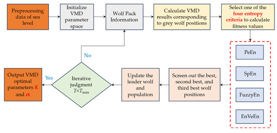
Figure 2.
Dynamic tuning of VMD parameters via four entropy criteria in GWO.
The original signal is then decomposed using VMD once each set of (K, α) parameters has been initialized. The fitness value of each wolf is determined by using the fitness function to assess the quality of the decomposition. The selection of the fitness function is the focus of our attention here. Four entropy criteria, namely permutation entropy (PeEn), sample entropy (SpEn), fuzzy entropy (FuzzyEn), and envelope entropy (EnVeEn), are selected. Through comprehensive evaluation from multiple perspectives, including randomness, regularity, structural stability, and envelope characteristics, more accurate searching for the optimal parameters of VMD by GWO is enabled, and the decomposition accuracy of sea level change data is thereby enhanced.
Next, the three wolves with the best fitness are selected as the best, second best, and third best based on fitness ranking. The leader wolf is updated, and other wolves are guided to search and update their own locations. Finally, the steps of calculating fitness values and updating positions are repeated. The iteration and output the (K, α) corresponding to the optimal wolf as the optimal parameter if the maximum number of iterations is reached or the fitness value tends to stabilize. Iterative convergence judgment is completed.
The most appropriate decomposition parameter configuration for sea level signals can be adaptively determined by dynamically adjusting the K and α parameters of VMD using GWO. This greatly increases the accuracy of VMD decomposition and successfully guarantees the performance of ensuing feature recognition tasks.
3.3. Deep Learning Prediction Model
After the optimal (K, α) parameters of the VMD model are obtained via the GWO algorithm, a solid foundation is laid for subsequent data feature mining by high-quality modal decomposition. The modal components obtained through optimized decomposition effectively retain the key information of the original signal, and problems of mode mixing and information loss are avoided. After the accurate deconstruction of the signal is completed, the construction of a prediction model with strong feature learning ability becomes the core link in transforming data value into prediction efficiency. Effective prediction models can not only deeply extract the implicit temporal patterns and associated features in modal components but also provide a reliable basis for trend prediction in practical scenarios. For this purpose, the CNN-BiGRU prediction model, which integrates a convolutional neural network (CNN) and bidirectional gated recurrent unit (BiGRU), is proposed to achieve high-precision prediction of processed data. The fusion structure of CNN-BiGRU is shown in Figure 3.
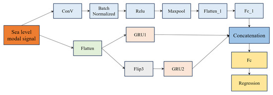
Figure 3.
The network structure of the CNN-BiGRU model.
3.3.1. Convolutional Neural Network
A CNN is employed to extract local features and spatial correlation information hidden in the modal signals of sea level changes [28]. Firstly, the feature matrix is convolved by multi-scale convolution kernels through sliding windows to capture local detail features of different dimensions. Then, the convolutional results are subsampled by the pooling layer, with data dimensionality and redundancy reduced, while key information is preserved. Ultimately, the integration and mapping of features are achieved through fully connected layers, forming more representative high-dimensional feature vectors. After being processed by CNN, high-quality feature information would be concatenated with BiGRU to serve as input, laying a key foundation for enhancing the accuracy of the overall prediction model.
3.3.2. Bidirectional Gated Recurrent Unit
By virtue of its bidirectional structural characteristics, parallel processing of sea level modal feature sequences in both forward and reverse directions is enabled by BiGRU. Temporal dependencies from the past to the present are captured by forward units, while correlation information from the future to the current is mined by reverse units [32]. Subsequently, the hidden states of the two are fused to form a comprehensive representation of temporal features. Next, hyperparameters such as learning rate, number of iterations, and batch size are set; the root mean square error is adopted as the loss function, and model parameters are iteratively updated using the Adam optimizer. Finally, the modal components of the test set are predicted using the trained model, and the predicted results of each modal component are superimposed to obtain the final predicted value of the original signal. The accuracy of sea level prediction is evaluated using multiple objective indicators.
3.4. Evaluation Metrics
Both factual and subjective visual indicators are available to assess how well sea level fluctuations are predicted. Changes in anticipated values and residual characteristics are the primary metrics used to assess subjective vision. A variety of numerical statistics data are evaluated using objective assessment indicators to analyze the effectiveness of approaches and techniques. Root mean square error (RMSE) [40], mean absolute error (MAE) [41], mean absolute percentage error (MAPE) [42], and Nash Sutcliffe efficiency (NSE) [43] are among the objective measures used for this study.
(1) Root mean square error
The average difference between expected sea level changes and actual observations is measured via root mean square error. The accuracy of the model increases with a smaller RMSE, which indicates a smaller difference between the actual sea level height and the anticipated value. The formula is expressed as
where n is the number of predicted samples. and are the actual observed and predicted values of sea level height at the i-th time point, respectively.
(2) Mean absolute error
The average absolute deviation between the observed value and the predicted value is represented by the average absolute error. The average prediction accuracy of traditional seasonal sea level changes is accurately reflected by MAE. It is described as
(3) Mean absolute percentage error
The data on sea level may differ in magnitude. The average proportion of prediction error to actual sea level height is represented by the MAPE value in sea level prediction, which places more focus on the relative magnitude of departure than absolute values.
(4) Nash Sutcliffe efficiency
The overall agreement between the anticipated and actual observed values is measured by the Nash Sutcliffe efficiency, which indicates how well the model captures data patterns and amplitudes. The model performs better when the NSE value is closer to 1. It can be described as
where is the average of sea level observations.
3.5. Implementation of Proposed Strategy
The sea level change prediction scheme for dynamically tuning VMD and CNN-BiGRU models is presented in Algorithm 1. Firstly, the preprocessing of original sea level time-series data is not limited to normalization and default value processing. Subsequently, the modal number K and penalty factor α parameters of the VMD model are optimized via the GWO algorithm. Envelope entropy (EnVeEn), permutation entropy (PeEn), fuzzy entropy (FuzzyEn), and sample entropy (SpEn) are adopted as fitness functions during the optimization process. The optimal fitness function, along with the corresponding K and α are determined by comparing the decomposition effects under different entropy values.
Then, VMD is used to decompose the preprocessed sea level data into multiple modal components based on the optimized parameter combination. Each component is divided into a training set and a testing set, and the input of the feature step size is compared. The features and sample outputs are input separately into the CNN-BiGRU model for model training. Local temporal features are extracted by the CNN module through 1D convolution. Bidirectional long-term dependencies are captured by the BiGRU module, and predicted values for each component are output through a fully connected layer. Finally, the predicted results of all modal components are superimposed and reconstructed to obtain the final predicted value of the original sea level change. The prediction accuracy is evaluated through multiple objective indicators.
| Algorithm 1. Dynamic tuning of variational mode decomposition and convolutional bidirectional gated recurrent unit for predicting sea level changes |
| Input: Monthly mean sea level data; VMD parameter ranges K, α; grey wolf population size pop; maximum iterations Tmax; CNN-BiGRU hyperparameters (kernel, maxpool, hidden, epochs, batch_size, L_rate); activation function; optimizer; tolerance tol; feature window size CSize. |
| Output: Predicted sea level time series; evaluation metrics (RMSE, MAE, MAPE, NSE). |
| 1: Preprocess data: normalization, missing value imputation, and outlier handling. |
| 2: Initialize the grey wolf population with random combinations of VMD parameters K, α. |
| 3: Iterative Optimization: |
| • Perform VMD decomposition for each parameter set. |
| • Evaluate fitness using selected entropy criterion (EnVeEn, PeEn, FuzzyEn, SpEn). |
| • Update grey wolf positions according to GWO rules. |
| 4: Select optimal VMD parameters K, α. |
| 5: Conduct multi-scale VMD decomposition using optimized parameters. |
| 6: For each intrinsic mode component: |
| • Extract features and partition data into training and testing sets. |
| • Train CNN-BiGRU model to learn spatial-temporal correlations. |
| • Generate mode-specific predictions. |
| 7: Aggregate predictions from all modes to produce the final sea level prediction. |
| 8: Evaluate performance using RMSE, MAE, MAPE, NSE, and other relevant metrics. |
4. Results
4.1. Datasets Description and Parameter Settings
The experimental data are sourced from the monthly mean sea level data provided by the Permanent Service for Mean Sea Level (PSMSL). Sea level change values are calculated from tide gauge observations via the revised local reference (RLR). Kanmen station in Zhejiang Province and Zhapo station in Guangdong Province, China, were selected as experimental sites by this study, with regional summary information presented in Figure 4. Both stations are situated at important economic and ecological intersections along the East China and South China coasts. Sea level changes at both stations are not only directly related to coastal disaster prevention and mitigation, ecological protection, and regional development planning, but also provide key data support for research on sea level change patterns and the formulation of response strategies along the coasts of China [44,45]. In addition, the data from the Zhapo site serves as a validation for the scalability and adaptability of the proposed solution. The data time span for the two stations ranges from January 1959 to November 2024 (a total of 65 years and 11 months), with data completeness rates of 98.9% for Kanmen and 98.2% for Zhapo, respectively. Missing values in the data are filled using nearest neighbor interpolation. The dataset is divided in chronological order, with the first 80% of the time-series data designated as the training set and the remaining 20% as the testing set (covering January 2012 to November 2024).
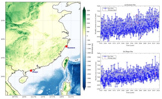
Figure 4.
Information on the research area and sea level time-series data of the stations.
The proposed sea level change prediction scheme mainly involves the setting of some key parameters for VMD, GWO, various entropy criteria, the CNN network, and the BiGRU model, as shown in Table 1. The excellent performance of the relevant parameters has been verified through subsequent experiments and discussions.

Table 1.
Parameter description and setting for the proposed prediction scheme of sea level changes.
4.2. Entropy Criterion Performance
To verify the effectiveness of different entropy criteria as fitness functions in solving optimal VMD combination parameters, a performance comparison analysis was conducted. CNN-BiGRU was adopted as the prediction model in the experiment, and the temporal feature length was set to 6. Selected fitness functions encompassed envelope entropy (EnVeEn), permutation entropy (PeEn), fuzzy entropy (FuzzyEn), and sample entropy (SpEn). In parameter configurations, the embedding dimension for each entropy was 3. The time delay for permutation entropy was configured as 1. The similarity tolerance for fuzzy entropy and sample entropy was 0.15 times the standard deviation of sea level change data, while the decay rate index for adjusting membership degree was configured as 2. The experimental results are presented in Figure 5 and Figure 6 and Table 2.
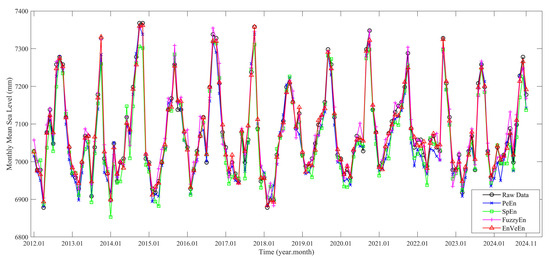
Figure 5.
The predictive performance of four entropy criteria on the test set.
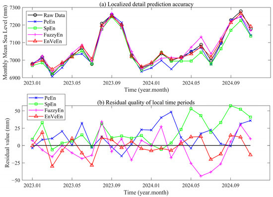
Figure 6.
Prediction quality of four entropy criteria in local time periods.
Table 2.
Performance evaluation indicators for four entropy criteria.
The prediction performance of monthly mean sea level changes from 2012 to 2024 is presented in Figure 5. Significant interannual fluctuations with 12 months are displayed in the original monthly mean sea level data. A comparative analysis of four entropy criteria (PeEn, SpEn, FuzzyEn, EnVeEn) reveals that EnVeEn achieves the optimal fitting performance for peaks, valleys, and fluctuation rhythms of monthly time-series data, and is more adapted to the dynamic complexity of sea level changes. The predictive capability of EnVeEn is able to effectively seize abrupt change characteristics and conduct nonlinear characterization of temporal information. In contrast, PeEn, SpEn, and FuzzyEn respectively exhibit drawbacks including underestimation of fluctuation amplitude, excessive flattening of trend fitting, and substantial deviation in peak-valley values.
The prediction quality of four entropy criteria from January 2023 to November 2024 is presented in Figure 6. In terms of prediction fitting, the prediction curve of EnVeEn achieves the highest fitting degree with the original sea level data. Key turning points, including the peak in September 2023 and the valley in early 2024, are captured most accurately. In terms of error stability, the smallest fluctuation amplitude of residual errors is observed for EnVeEn, with most values within ±30 mm. In contrast, more obvious fitting deviations and more severe residual error fluctuations are exhibited by the three entropy criteria: PeEn, SpEn, and FuzzyEn. For PeEn, a value approaching 50 mm was recorded in March 2024. For SpEn, a value exceeding 50 mm was observed in May 2024. For FuzzyEn, an error of nearly 50 mm was noted in June 2024. These results demonstrate that EnVeEn excels in capturing short-term dynamic changes in monthly mean sea level and exhibits superior predictive performance within this local time period.
Table 2 demonstrates that all four entropy criteria exhibit good predictive performance in the test set. The overall prediction results are highly satisfactory and effectively identify optimal combination parameter values for each criterion. In contrast, the performance indicators of SpEn are slightly inferior. The RMSE of EnVeEn is 33.3% lower than its counterpart for FuzzyEn, which indicates a significant improvement in its capacity to control extreme errors. With regard to the MAE metric, this further validates the excellent predictive stability of EnVeEn. In terms of the NSE metric, the explanatory power of EnVeEn for monthly mean sea level fluctuations is closer to 1.
4.3. Prediction Quality of Deep Learning Models
To verify performance differences among deep learning models in sea level change time series prediction tasks, experimental analysis is conducted as follows. EnVeEn with optimal performance is selected as the fitness function. Temporal feature length is configured as 6. LSTM, GRU, CNN-BiLSTM, and CNN-BiGRU are adopted as comparative models. Experimental results are presented in Figure 7 and Figure 8 and Table 3.
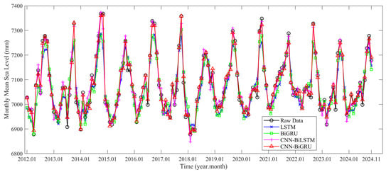
Figure 7.
Long-term predictive capability of various deep learning models on the test set.
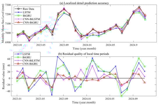
Figure 8.
Prediction quality of various deep learning models in local time periods.
Table 3.
Objective evaluation metric performance of various deep learning models.
Prediction fitting effects for the monthly mean sea level from 2012 to 2024 are presented in Figure 7. Within these effects, the prediction curve of the CNN-BiGRU model achieves a significantly superior fit with the original monthly mean sea level data. Trend inflection points, including annual peak and interannual valley values in August and September, are captured most accurately. LSTM, constrained by memory limitations in unidirectional temporal modeling, exhibits more notable fitting deviations during extreme peak fluctuations or complex periods. Meanwhile, BiGRU, limited by insufficient multi-scale feature extraction, shows similar deviations in such scenarios. Additionally, CNN-BiLSTM, hindered by characterization weaknesses in cyclic structures, also demonstrates more significant fitting biases during these periods. Such observations validate the advantages of the convolutional and bidirectional gated loop architecture. Multi-scale fluctuation features are extracted by CNN, while long-range dependencies are bidirectionally characterized by BiGRU. The synergy between these two components enhances the adaptability of CNN-BiGRU to the periodic and nonlinear characteristics of sea level, thereby exhibiting stronger dynamic tracking capabilities in long-term prediction.
The prediction quality of various deep learning models within locally zoomed time regions is presented in Figure 8. Analysis of prediction fitting (Figure 8a) and residual error (Figure 8b) reveals that the predictive performance of CNN-BiGRU is significantly superior to that of LSTM, BiGRU, and CNN-BiLSTM. In terms of key inflection point fitting, the trend of the peak in October 2023, valley in July 2024, and subsequent rebound is captured most accurately by CNN-BiGRU. The curve achieves the highest fitting degree with the original data. In terms of error stability, the smallest fluctuation amplitude of residual errors is observed for CNN-BiGRU. In contrast, LSTM, BiGRU, and CNN-BiLSTM not only exhibit significant fitting biases but also show more severe fluctuations in residual errors, with multiple residuals even exceeding 40 mm. Such observations validate the architectural advantage of convolution-based extraction of multi-scale features and bidirectional gated cyclic characterization of temporal dependencies, enhancing the capacity of CNN-BiGRU for stronger detail tracking and error control in short-term dynamic prediction of monthly mean sea level.
Predictive performance of the four deep learning models for the monthly mean sea level is shown in Table 3, which gradually improves with architectural iteration, progressing from LSTM to CNN-BiGRU. In contrast, the weakest performance across indicators is exhibited by LSTM, attributed to memory limitations in unidirectional time series modeling. The RMSE of CNN-BiGRU is 23.7% lower than that of CNN-BiLSTM, underscoring stronger control over extreme errors. Optimization in MAE further validates the capacity of CNN-BiGRU to suppress average deviations. Compared to the high-performing CNN-BiLSTM model, the MAPE decreases from 0.198 to 0.151, indicating a reduced proportion of relative error. The NSE of CNN-BiGRU approaches 0.986, reflecting stronger explanatory power for sea level fluctuations. Comprehensive performance across indicators reflects the complementary mechanism of the CNN-BiGRU model, which integrates convolutional anchored wave processing and bidirectional gated weaving of time series correlations, along with precise deconstruction capacity for periodic sea level fluctuations and nonlinear distortions.
5. Discussion
5.1. Evaluation at Different Time Steps
To reveal the regulatory law of feature input length on the predictive performance of the constructed fusion model, the following experiments were conducted. EnVeEn with optimal performance was adopted as the fitness function. Based on the CNN-BiGRU prediction model, input step sizes for monthly scale features were set to 3, 6, 12, and 18 months, and the impact of time step size on the accuracy of monthly mean sea level change prediction was systematically investigated. Experimental results are presented in Figure 9.
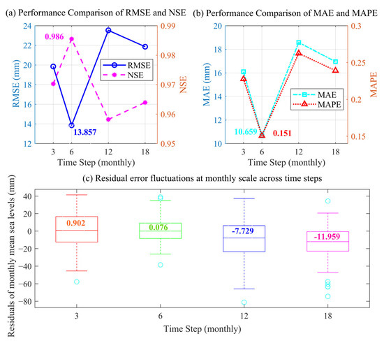
Figure 9.
Prediction performance under feature inputs at different time steps.
Performance of the proposed fusion scheme is shown in Figure 9 to be optimal overall when the time step is 6 months. Figure 9a illustrates that the RMSE value falls below 14 mm while the NSE exceeds 0.98. Synchronization of MAE and MAPE values in Figure 9b reaches the minimum, reflecting the optimal ratio of average absolute deviation to relative error. Additionally, the box plot in Figure 9c further confirms that residual fluctuation with a 6-month step size is the narrowest, featuring a median box size of 0.076 mm and minimal extreme error. Deterioration in all indicators is observed when the step size deviates from 6 months, including 3, 12, and 18 months. A step size that is too short (3 months) leads to error amplification, attributed to insufficient capture of cyclic correlations.
Excessively long step lengths (12 or 18 months) may induce increases in RMSE and MAE values, caused by interference from redundant temporal information or loss of critical short-term fluctuations. At 12 months, RMSE, MAE, and MAPE reach their peaks, whereas NSE decreases to its lowest level. The residual fluctuation with an 18-month step size intensifies, and box expansion is significant, with a median value of −11.959 mm. This indicates that the 6-month step size perfectly matches the temporal characteristics of interannual nested short-term fluctuations in monthly mean sea level, achieving a balance between capturing cyclic correlations and preserving detailed fluctuations.
5.2. Monthly-Scale Statistical Prediction Performance
To investigate the predictive performance of various entropy criteria and deep learning models at the monthly scale, we conducted a statistical analysis of their prediction quality from January 2012 to November 2024. As shown in Figure 10 and Figure 11, the prediction quality and RMSE prediction performance for each month are displayed, respectively.
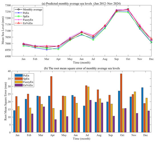
Figure 10.
Prediction performance of various entropies on a monthly statistical scale.
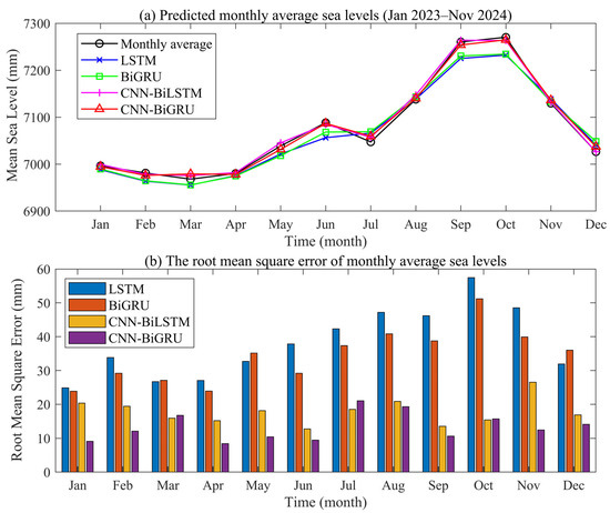
Figure 11.
Prediction performance of various deep learning models on a monthly statistical scale.
- (1)
- Performance of entropy criteria across each month
Statistical quality of various entropies across each month is presented in Figure 10, with EnVeEn exhibiting the best predictive performance among the four entropy methods. In temporal trend fitting, the predicted curve of EnVeEn achieves the highest fitting degree with the true monthly mean sea level, and key turning points, including the October peak and intraseasonal fluctuations, are captured most accurately. Long-term prediction bias for SpEn accumulates continuously, with curve deviation being the most notable.
Monthly statistics of root mean square error (RMSE) further confirm that EnVeEn exhibits the lowest RMSE values and smoothest fluctuations in most months, including April and October, reflecting precise adaptation to periodic rhythm and local fluctuation characteristics of monthly sea level. Prediction errors for PeEn and FuzzyEn fall in the middle range. However, SpEn exhibits the poorest overall prediction stability due to frequent extreme errors, particularly in performance at the extreme peak in October. This result indicates that the envelope feature-matching mechanism of EnVeEn is more consistent with the gradual periodic law of monthly mean sea level, and stronger dynamic tracking and error control capabilities are exhibited in long-term forecasting.
- (2)
- Performance of deep learning models across each month
Statistical quality of each deep learning model across each month is presented in Figure 11, with monthly scale prediction performance of the CNN-BiGRU model being significantly superior to that of LSTM, BiGRU, and CNN-BiLSTM. In temporal trend capture, the predicted curve of CNN-BiGRU achieves the highest fitting degree with the true monthly mean sea level, and the predicted curve maintains fitting with the true value throughout the entire cycle. Capture accuracy for key turning points, including the October peak and intraseasonal fluctuations, is particularly notable. Due to memory decay in unidirectional temporal flow, continuous accumulation of bias in long-term prediction is exhibited by LSTM, with the curve deviation trend being most significant.
The monthly distribution of root mean square error further confirms that the error bars of CNN-BiGRU are generally shorter with narrower fluctuations. Even during the peak error period in October, the error of CNN-BiGRU remains relatively low, perfectly adapting to the characteristics of periodic rhythm and nonlinear distortion in the monthly sea level. Prediction errors of BiGRU and CNN-BiLSTM fall in the middle range. Meanwhile, sharp increases in the RMSE of LSTM and BiGRU are observed in extreme months, revealing stability weaknesses in long-term forecasting. The root cause of such performance differences lies in the architecture combining multi-scale feature anchoring and bidirectional temporal binding, which endows CNN-BiGRU with stronger dynamic tracking and error convergence capabilities in monthly mean sea level prediction.
- (3)
- Seasonal fluctuation characteristics
The seasonal variation in prediction errors is primarily influenced by the interplay between the periodicity and extremity of climatic driving factors. As shown in Figure 4, sea level changes during March to May (spring) are relatively stable, due to the transition between monsoon seasons and steady river discharge. Storm surge activity is minimal, and monthly fluctuations remain small (±20 mm), resulting in low nonlinearity and high modal stability. Figure 10 and Figure 11 display that these favorable conditions enable our proposed model to achieve the highest prediction accuracy, with RMSE less than 15 mm. In contrast, during July to August (summer), frequent typhoons in the northwestern Pacific trigger step-like sea level surges of 30 to 50 mm. Although the dynamically optimized VMD can decompose these abrupt modes, the CNN-BiGRU exhibits a slight lag in fitting aperiodic disturbances, thereby increasing prediction errors by 2 to 3 mm. From December to February (winter), frequent cold surges induced setup events, characterized by short duration and high suddenness, and introduced additional noise into sea level signals, leading to larger residual fluctuations. Particularly notable is the summer typhoon season, when the intensity of sea level disturbances and the degree of nonlinearity reach their annual peak, accompanied by increased mode mixing in VMD decomposition, ultimately resulting in the highest prediction errors of the year, with peak RMSE reaching 20 mm. These patterns indicate that the spatiotemporal clustering of extreme climatic events significantly enhances the complexity of sea level dynamics and is a key factor affecting the seasonal performance of the forecasting model.
5.3. Extended Adaptability
To verify the scalability of the proposed scheme, sea level data corrected by the tide gauge at Zhapo station were analyzed. In Figure 12a, the monthly forecast values of BIGRU exhibit notable magnitude discrepancies. The prediction curve of the CNN-BiGRU model aligns more closely with the interannual fluctuations of the original data, and its trend tracking accuracy at extreme values is remarkable. Residual analysis in Figure 12b reveals that the residuals of CNN-BiGRU are more stably concentrated around 0, with errors of within ±30 mm in most time periods. In contrast, the residuals of BiGRU fluctuate drastically, with errors exceeding 50 mm in October 2017 and October 2021. This difference arises from the integration by CNN-BiGRU of spatial feature extraction based on CNN and temporal dependency modeling enabled by BiGRU, which allows for more accurate dissection of the nonlinear laws governing sea level changes. Such an advantageous characteristic is not confined to the sea level change data of Kanmen station; instead, it enables the proposed scheme to outperform other techniques significantly in both trend fitting accuracy and error stability for sea level prediction at Zhapo station, thereby demonstrating stronger scalability.
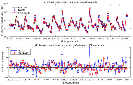
Figure 12.
Analysis of prediction quality at Zhapo station to verify the adaptability of the proposed scheme.
Figure 13 presents the statistical error characteristics of predictions and kernel density scatter fitting patterns for the Zhapo site from January 2012 to November 2024. The R2 index is incorporated to quantify the agreement between predicted values of the models and actual values [46]. Figure 13a compares the BIGRU and CNN-BiGRU models via residual statistical distributions. The residual distribution of BiGRU is discrete, with RMSE = 21.491 mm and MAE = 16.403 mm. By contrast, residuals of CNN-BiGRU are more concentrated, with RMSE = 16.230 mm and MAE = 13.129 mm. These indicator values collectively reflect the prediction accuracy, error distribution pattern, and overall fitting performance of CNN-BiGRU in sea level change prediction. In the kernel density scatter plot of Figure 13b, predicted values of CNN-BiGRU align more closely with actual values, with R2 = 0.9805 outperforming that of 0.9766. These two types of statistical results jointly reveal that CNN-BiGRU exhibits smaller errors and a higher fitting degree in sea level prediction at Zhapo Station, thus effectively verifying the scalability and adaptability of the model.
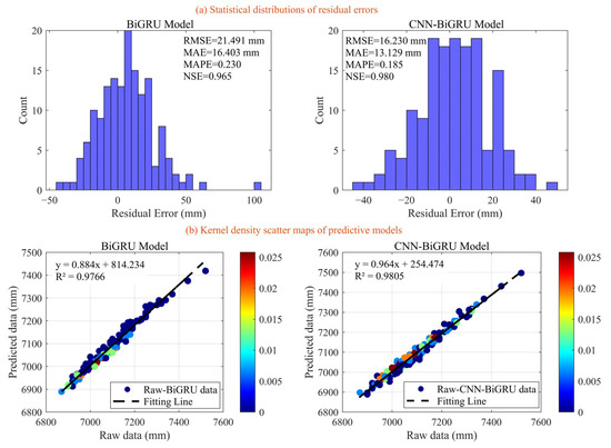
Figure 13.
Statistical characteristics and scatter fitting features of the Zhapo station to verify the adaptability of the proposed scheme.
5.4. Differences in Site Prediction and Regional Dynamics Insights
Figure 5, Figure 7, Figure 12 and Figure 13 show that the prediction accuracy at Kanmen Station (Zhejiang, along the East China Sea coast) is significantly higher than that at Zhapo Station (Guangdong, along the South China Sea coast). Kanmen Station achieves an RMSE of 13.857 mm and an NSE of 0.986, compared to an RMSE of 16.230 mm and an NSE of 0.980 at Zhapo Station. Moreover, the residual fluctuations at Kanmen Station (±15 mm) are notably smaller than those at Zhapo Station (±20 mm), indicating superior prediction stability of the model at the East China Sea coastal site.
The observed site-specific differences can be primarily attributed to the coupling between data characteristics and regional driving mechanisms. As noted by Mu et al., due to seawater thermal expansion and seasonal regulation from the Yangtze River runoff [6], the monthly mean sea level data at Kanmen Station exhibit low nonlinearity and strong periodic regularity, with a 6-month cycle accounting for up to 75%. This characteristic is well aligned with the selection of a feature window size of 6, enabling the CNN-BiGRU model to more accurately capture the combined features of stable periodicity and weak fluctuations. In contrast, Zhapo Station, located in the northwestern South China Sea, is subject to multiple unstable driving factors. First, typhoon activity in the northwestern Pacific induces storm surges during July to September each year, causing short-term sea level fluctuations of up to ±40 mm [5]. Second, interannual variations in the South China Sea circulation, such as fluctuations in the strength of the warm current, lead to sea level anomalies. These factors result in highly nonlinear, abruptly changing, and fragmented periodic patterns at Zhapo Station, where the 6-month cycle accounts for only 55%. Even after VMD dynamic optimization, there are still 1–2 high noise modes, which increase the prediction error. In addition, data integrity and observation environment also have an impact on the results: the data integrity of Kanmen Station (98.9%) is higher than that of Zhapo Station (98.2%), and it is located on the outer side of Hangzhou Bay. The tide gauge is less affected by coastal sediment deposition, and the observation data have a high signal-to-noise ratio [47]. However, Zhapo Station is close to the Pearl River Estuary, and due to the impact of suspended sediment brought by runoff, there is a small systematic deviation in some monthly observation data [48]. Despite the interpolation correction, it still introduces a slight error into the prediction. These factors work together to result in a significant difference in predictive performance between the two sites.
Significant differences exist in sea level dynamics between the East China Sea and the South China Sea. The northern East China Sea is characterized by a combination of long-term trends and stable periodicity, primarily driven by persistent climatic factors such as global warming and monsoons, resulting in high predictability. In contrast, the northwestern South China Sea exhibits a compound dynamic pattern of stable trends superimposed with episodic disturbances, strongly influenced by extreme events like typhoons and oceanic circulation anomalies, leading to greater prediction complexity. This contrast suggests that future regional sea level forecasting models should be tailored to the specific characteristics of each sea area: in the East China Sea, long-term early warning systems can be developed based on strong periodic signals, while in the South China Sea, models should integrate real-time dynamic factors such as typhoon tracks and circulation intensity to establish a dual-response framework that combines routine forecasting with emergency adjustment for extreme events, thereby supporting more accurate and adaptive coastal protection strategies.
6. Conclusions
To address the persistent challenges of mode aliasing and limited accuracy in sea level prediction, this study proposes a sea level prediction scheme combining dynamic optimization of variational mode decomposition and convolutional bidirectional gated recurrent units. The main contributions are summarized as follows:
- (1)
- Dynamic Optimization of Signal Decomposition: A dynamic VMD optimization strategy was developed to mitigate mode aliasing inherent in conventional decomposition methods. This approach reduced the RMSE of predictions by up to 33% (from 20.790 mm to 13.857 mm) and achieved an NSE of 0.986, establishing a high-fidelity foundation for subsequent forecasting.
- (2)
- Hybrid CNN-BiGRU Architecture for Feature Extraction: The CNN-BiGRU model captures both local spatial features and long-range bidirectional temporal dependencies within decomposed sea level components while accurately characterizing complex periodic fluctuations and nonlinear distortions, thereby improving dynamic tracking and error convergence.
- (3)
- Comprehensive Evaluation Protocol: Beyond standard accuracy metrics, a systematic evaluation protocol incorporating entropy criterion selection and feature time step analysis was employed. An optimal feature time step of six months was identified, which provided actionable guidance for robust model implementation.
- (4)
- Regional Predictability and Tailored Modeling Guidance: Comparative analysis revealed pronounced site-specific differences. The East China Sea (Kanmen Station), characterized by stable periodicity, exhibited high predictability, whereas the South China Sea (Zhapo Station), influenced by typhoons and circulation anomalies, presented greater challenges. These findings underscore the need to tailor forecasting models: leveraging long-term periodic signals for early warning in stable regions, while incorporating real-time dynamic factors to support adaptive coastal management in complex environments.
Validation across both sites confirms the robustness and superiority of the proposed scheme, demonstrating its capacity to capture nuanced regional dynamics. Future work will focus on integrating multi-source data—including meteorological and oceanographic observations, storm surge models, climate scenario projections, and satellite altimetry—to better capture extreme events and further enhance the model’s adaptability and generalizability.
Author Contributions
Methodology, Z.Z. and P.Z.; formal analysis, W.R.; data curation, Z.Z.; writing—original draft preparation, Z.Z. and P.Z.; writing—review and editing, W.R.; visualization, J.C.; supervision, P.Z. and J.C.; funding acquisition, G.C., P.Z. All authors have read and agreed to the published version of the manuscript.
Funding
This study was funded by the National Natural Science Foundation of China, grant number 42274012.
Data Availability Statement
The monthly mean sea level data used in this study were obtained from the PSMSL website (https://psmsl.org/, accessed on 30 May 2025).
Acknowledgments
The authors thank the anonymous reviewers for their constructive suggestions.
Conflicts of Interest
The authors declare no conflicts of interest.
References
- Bagnell, A.; DeVries, T. Global Mean Sea Level Rise Inferred from Ocean Salinity and Temperature Changes. Geophys. Res. Lett. 2023, 50, e2022GL101004. [Google Scholar] [CrossRef]
- Palmer, M.D.; Harrison, B.J.; Gregory, J.M.; Hewitt, H.T.; Lowe, J.A.; Weeks, J.H. A Framework for Physically Consistent Storylines of UK Future Mean Sea Level Rise. Clim. Change 2024, 177, 106. [Google Scholar] [CrossRef]
- Hamlington, B.D.; Fournier, S.; Thompson, P.R.; Marcos, M. Sea Level Rise in 2024. Nat. Rev. Earth Environ. 2025, 6, 246–248. [Google Scholar] [CrossRef]
- Abdelhafez, M.A.; Mahmoud, H.N.; Ellingwood, B.R. Adjusting to the Reality of Sea Level Rise: Reshaping Coastal Communities through Resilience-Informed Adaptation. Clim. Change 2024, 177, 110. [Google Scholar] [CrossRef]
- Cantelon, J.A.; LeRoux, N.K.; Mulligan, R.P.; Swatridge, L.; Kurylyk, B.L. Interrelated Coastal Flooding, Erosion, and Groundwater Salinization on a Barrier Island during Hurricane Fiona. J. Geophys. Res. Earth Surf. 2024, 129, e2023JF007551. [Google Scholar] [CrossRef]
- Mu, D.; Xu, T.; Yan, H. Sea Level Rise along China Coast from 1950 to 2020. Sci. China Earth Sci. 2024, 67, 802–810. [Google Scholar] [CrossRef]
- Liu, H.; Cheng, X.; Qin, J.; Zhou, G.; Jiang, L. The Dynamic Mechanism of Sea Level Variations in the Bohai Sea and Yellow Sea. Clim. Dyn. 2023, 61, 2937–2947. [Google Scholar] [CrossRef]
- Huang, W.-C.; Liu, W.-C.; Liu, H.-M. Uncertainty Analysis of Overflow Due to Sea Dike Failure during Typhoon Events. J. Mar. Sci. Eng. 2025, 13, 573. [Google Scholar] [CrossRef]
- Liu, W.; Fujii, K.; Maruyama, Y.; Yamazaki, F. Inundation Assessment of the 2019 Typhoon Hagibis in Japan Using Multi-Temporal Sentinel-1 Intensity Images. Remote Sens. 2021, 13, 639. [Google Scholar] [CrossRef]
- Sun, Q.; Wan, J.; Liu, S.; Jiang, J.; Muhammad, Y. A New Decomposition Model of Sea Level Variability for the Sea Level Anomaly Time Series Prediction. J. Oceanol. Limnol. 2023, 41, 1629–1642. [Google Scholar] [CrossRef]
- Raj, N.; Gharineiat, Z.; Ahmed, A.A.M.; Stepanyants, Y. Assessment and Prediction of Sea Level Trend in the South Pacific Region. Remote Sens. 2022, 14, 986. [Google Scholar] [CrossRef]
- Rashid, M.M.; Wahl, T. Predictability of Extreme Sea Level Variations along the U.S. Coastline. J. Geophys. Res. Oceans 2020, 125, e2020JC016295. [Google Scholar] [CrossRef]
- Wang, F.; Shen, Y.; Geng, J.; Chen, Q. Global Mean Sea Level Change Projections up to 2100 Using a Weighted Singular Spectrum Analysis. J. Mar. Sci. Eng. 2024, 12, 2124. [Google Scholar] [CrossRef]
- Ahmadi, F.; Tohidi, M.; Sadrianzade, M. Streamflow Prediction Using a Hybrid Methodology Based on Variational Mode Decomposition (VMD) and Machine Learning Approaches. Appl. Water Sci. 2023, 13, 135. [Google Scholar] [CrossRef]
- Shen, W.; Ying, Z.; Zhao, Y.; Wang, X. Significant Wave Height Prediction in Monsoon Regions Based on the VMD-CNN-BiLSTM Model. Front. Mar. Sci. 2024, 11, e1503552. [Google Scholar] [CrossRef]
- Zhang, Y.; Zhang, T.; Shen, W.; Ou, Z.; Zhang, J. Economic Loss Assessment of Typhoon-Induced Storm Surge Disasters in the South China Sea Based on GSA-BP Model. Front. Earth Sci. 2023, 11, e1258524. [Google Scholar] [CrossRef]
- Gholami Rostam, M.; Sadatinejad, S.J.; Malekian, A. Precipitation Forecasting by Large-Scale Climate Indices and Machine Learning Techniques. J. Arid. Land 2020, 12, 854–864. [Google Scholar] [CrossRef]
- Riahi-Madvar, H.; Dehghani, M.; Memarzadeh, R.; Gharabaghi, B. Short to Long-Term Forecasting of River Flows by Heuristic Optimization Algorithms Hybridized with ANFIS. Water Resour. Manag. 2021, 35, 1149–1166. [Google Scholar] [CrossRef]
- Elshewey, A.M. Enhancing Crop Yield Prediction Based on Dove Optimization Algorithm and Gradient Boosting Model. Signal Image Video Process. 2025, 19, 951. [Google Scholar] [CrossRef]
- Elshewey, A.M.; Osman, A.M. Orthopedic Disease Classification Based on Breadth-First Search Algorithm. Sci. Rep. 2024, 14, 23368. [Google Scholar] [CrossRef]
- Elshewey, A.M.; Abed, A.H.; Khafaga, D.S.; Alhussan, A.A.; Eid, M.M.; El-kenawy, E.-S.M. Enhancing Heart Disease Classification Based on Greylag Goose Optimization Algorithm and Long Short-Term Memory. Sci. Rep. 2025, 15, 1277. [Google Scholar] [CrossRef]
- Elshewey, A.M.; Alhussan, A.A.; Khafaga, D.S.; Elkenawy, E.-S.M.; Tarek, Z. EEG-Based Optimization of Eye State Classification Using Modified-BER Metaheuristic Algorithm. Sci. Rep. 2024, 14, 24489. [Google Scholar] [CrossRef] [PubMed]
- Sithara, S.; Pramada, S.K.; Thampi, S.G. Sea Level Prediction Using Climatic Variables: A Comparative Study of SVM and Hybrid Wavelet SVM Approaches. Acta Geophys. 2020, 68, 1779–1790. [Google Scholar] [CrossRef]
- Zahura, F.T.; Goodall, J.L.; Sadler, J.M.; Shen, Y.; Morsy, M.M.; Behl, M. Training Machine Learning Surrogate Models from a High-Fidelity Physics-Based Model: Application for Real-Time Street-Scale Flood Prediction in an Urban Coastal Community. Water Resour. Res. 2020, 56, e2019WR027038. [Google Scholar] [CrossRef]
- Yu, H.; Gong, H.; Chen, B. Analysis of the Superposition Effect of Land Subsidence and Sea-Level Rise in the Tianjin Coastal Area and Its Emerging Risks. Remote Sens. 2023, 15, 3341. [Google Scholar] [CrossRef]
- Bay, Y.Y.; Yearick, K.A. Machine Learning vs Deep Learning: The Generalization Problem. arXiv 2024, arXiv:2403.01621. [Google Scholar] [CrossRef]
- Tumse, S.; Alcansoy, U. Statistical and Deep Learning Approaches in Estimating Present and Future Global Mean Sea Level Rise. Nat. Hazard. 2025, 121, 10377–10404. [Google Scholar] [CrossRef]
- Uluocak, I. Comparative Study of Multivariate Hybrid Neural Networks for Global Sea Level Prediction through 2050. Environ. Earth Sci. 2025, 84, 79. [Google Scholar] [CrossRef]
- Ning, P.; Zhang, C.; Zhang, X.; Jiang, X. Short- to Medium-Term Sea Surface Height Prediction in the Bohai Sea Using an Optimized Simple Recurrent Unit Deep Network. Front. Mar. Sci. 2021, 8, 672280. [Google Scholar] [CrossRef]
- El-Rashidy, N.; Tarek, Z.; Elshewey, A.M.; Shams, M.Y. Multitask Multilayer-Prediction Model for Predicting Mechanical Ventilation and the Associated Mortality Rate. Neural Comput. Appl. 2025, 37, 1321–1343. [Google Scholar] [CrossRef]
- Raj, N.; Brown, J. Prediction of Mean Sea Level with GNSS-VLM Correction Using a Hybrid Deep Learning Model in Australia. Remote Sens. 2023, 15, 2881. [Google Scholar] [CrossRef]
- Li, X.; Zhou, S.; Wang, F. A CNN-BiGRU Sea Level Height Prediction Model Combined with Bayesian Optimization Algorithm. Ocean Eng. 2025, 315, 119849. [Google Scholar] [CrossRef]
- Yang, Y.; Cheng, Q.; Tsou, J.-Y.; Wong, K.-P.; Men, Y.; Zhang, Y. Multiscale Analysis and Prediction of Sea Level in the Northern South China Sea Based on Tide Gauge and Satellite Data. J. Mar. Sci. Eng. 2023, 11, 1203. [Google Scholar] [CrossRef]
- Huang, S.; Nie, H.; Jiao, J.; Chen, H.; Xie, Z. Tidal Level Prediction Model Based on VMD-LSTM Neural Network. Water 2024, 16, 2452. [Google Scholar] [CrossRef]
- Wang, L.; Liao, S.; Wang, S.; Yin, J.; Li, R.; Guan, J. Real-Time Prediction of Port Water Levels Based on EMD-PSO-RBFNN. Front. Mar. Sci. 2025, 12, 1537696. [Google Scholar] [CrossRef]
- Chen, H.; Lu, T.; Huang, J.; He, X.; Sun, X. An Improved VMD–EEMD–LSTM Time Series Hybrid Prediction Model for Sea Surface Height Derived from Satellite Altimetry Data. J. Mar. Sci. Eng. 2023, 11, 2386. [Google Scholar] [CrossRef]
- Tiu, E.S.K.; Huang, Y.F.; Ng, J.L.; AlDahoul, N.; Ahmed, A.N.; Elshafie, A. An Evaluation of Various Data Pre-Processing Techniques with Machine Learning Models for Water Level Prediction. Nat. Hazard. 2022, 110, 121–153. [Google Scholar] [CrossRef]
- Wu, J.; Guo, J.; Wu, J. Physics-Informed Hybrid Model for Scour Evolution Prediction around Pile Foundations under Tidal Currents. Phys. Fluids 2025, 37, e0267721. [Google Scholar] [CrossRef]
- Li, H.; Zhang, L.; Yao, Y.; Zhang, Y. Prediction of Water Levels in Large Reservoirs Base on Optimization of Deep Learning Algorithms. Earth Sci. Inf. 2024, 18, 121. [Google Scholar] [CrossRef]
- Li, A.; Zhu, X.; Zhang, Y.; Ren, S.; Zhang, M.; Zu, Z.; Wang, H. Recent Improvements to the Physical Model of the Bohai Sea, the Yellow Sea and the East China Sea Operational Oceanography Forecasting System. Acta Oceanolog. Sin. 2021, 40, 87–103. [Google Scholar] [CrossRef]
- Van Katwyk, P.; Fox-Kemper, B.; Seroussi, H.; Nowicki, S.; Bergen, K.J. A Variational LSTM Emulator of Sea Level Contribution from the Antarctic Ice Sheet. J. Adv. Model. Earth Syst. 2023, 15, e2023MS003899. [Google Scholar] [CrossRef]
- Alenezi, N.; Alsulaili, A.; Alkhalidi, M. Prediction of Sea Level in the Arabian Gulf Using Artificial Neural Networks. J. Mar. Sci. Eng. 2023, 11, 2052. [Google Scholar] [CrossRef]
- Adwait; Roshni, T. Mean Sea Level Modelling Using the Neural Network along the Chennai Coast. J. Water Clim. Change 2022, 14, 66–82. [Google Scholar] [CrossRef]
- Feng, J.; von Storch, H.; Jiang, W.; Weisse, R. Assessing Changes in Extreme Sea Levels along the Coast of China. J. Geophys. Res. Oceans 2015, 120, 8039–8051. [Google Scholar] [CrossRef]
- Zheng, Z.; Li, G.; Tang, C.; Zhou, X. Mean Sea Level Changes near Weizhou Island from 1969 to 2010. J. Ocean Univ. China 2014, 13, 369–374. [Google Scholar] [CrossRef]
- Karsavran, Y.; Erdik, T.; Ozger, M. An Improved Technique for Streamflow Forecasting between Turkish Straits. Acta Geophys. 2024, 72, 2831–2842. [Google Scholar] [CrossRef]
- Li, S.; Wahl, T.; Fang, J.; Liu, L.; Jiang, T. High-Tide Flooding along the China Coastline: Past and Future. Earth’s Future 2023, 11, e2022EF003225. [Google Scholar] [CrossRef]
- Li, B.; Cai, H.; Li, G.; Liu, J.; She, Z.; Wang, Y.; Ou, S.; Liu, F.; Zhao, T.; Lin, K. A General Unit Hydrograph Theory for Water Level and Tidal Range Distributions in the Modaomen Estuary, China. J. Hydrol. 2024, 643, 131933. [Google Scholar] [CrossRef]
Disclaimer/Publisher’s Note: The statements, opinions and data contained in all publications are solely those of the individual author(s) and contributor(s) and not of MDPI and/or the editor(s). MDPI and/or the editor(s) disclaim responsibility for any injury to people or property resulting from any ideas, methods, instructions or products referred to in the content. |
© 2025 by the authors. Licensee MDPI, Basel, Switzerland. This article is an open access article distributed under the terms and conditions of the Creative Commons Attribution (CC BY) license (https://creativecommons.org/licenses/by/4.0/).