Hindcasting Extreme Significant Wave Heights Under Fetch-Limited Conditions with Tree-Based Models

Abstract

Accurately hindcasting waves in semi-enclosed, fetch-limited basins remains challenging for reanalysis models, which tend to underestimate storm peaks near the coast. We developed interpretable ML models for Rijeka Bay (northern Adriatic) using only wind observations from two land-based wind stations to predict buoy H_m0 measurements spanning 2009–2011 (testing) and 2019–2021 (training and validation). The tested tree-based models included Random Forest, XGBoost, and Explainable Boosting Machine. This study introduces a novel approach in the literature by employing weighted schemes and feature engineering to enhance the predictive performance of interpretable, low-complexity machine learning models in hindcasting waves. Representing wind direction as sine–cosine components generally reduced RMSE and BIAS relative to traditional speed–direction inputs, while an exponential sample weight scheme that emphasized storm waves halved extreme H_m0 underprediction without inflating overall RMSE. The best-performing model, a Random Forest model, achieved an RMSE of 0.096 m and a correlation of 0.855 on the unseen test set—30% lower overall RMSE and 50% lower extreme wave RMSE than the MEDSEA and COEXMED hindcasts. Additionally, the underprediction was reduced by 90% compared to these reanalysis models. The method offers a computationally lightweight, transferable supplement to numerical wave guidance for coastal engineering and harbor operations.

1. Introduction

Accurate hindcasting of wave conditions, particularly significant wave heights (H_s), is essential for coastal and offshore engineering design [1,2], maritime operations [3], and coastal hazard mitigation [4,5,6]. Hindcasts reconstruct historical wave climates at high temporal resolution (often hourly), providing comprehensive datasets vital for coastal infrastructure design [7]. Such extensive datasets allow for confident long-term forecasting of significant wave heights and the determination of return periods (e.g., 50 years and 100 years). Reliable long-term wave databases are especially important for coastal seas, where data availability is generally limited compared to deeper ocean regions [8].

Long-term wave hindcasts are particularly valuable in fetch-limited seas—such as the Mediterranean or Adriatic—for designing coastal structures and understanding wave climate variability. Fetch-limited wave generation refers to conditions where wind-driven waves cannot reach full development because the wind’s fetch (distance) or duration is limited. In these enclosed basins, where wave buoys are often deployed only temporarily, and not for long-term campaigns [9], engineers frequently lack sufficiently long measurement records [7,10]. Hindcasting using historical wind and environmental data can extend short wave records, supporting design and safety assessments [10].

Traditionally, empirical models (e.g., SMB [11,12]), physics-based numerical models [13,14,15], or statistical analyses have been used [16,17]. However, these empirical methods often exhibit large uncertainties in fetch-limited conditions due to oversimplifications or sensitivity to complex local geographies [18,19], like island shielding effects in Aegean Sea [20]. On the other hand, wave numerical models require detailed inputs (e.g., bathymetry, white-capping coefficients, bed friction, etc.) and significant computational resources but provide physics-based predictions, especially wave reanalysis models [21,22,23]. Although the MEDSEA reanalysis model offers the most detailed spatial and temporal resolution of any Copernicus numerical model reanalysis in the Mediterranean, Korres et al. [21] still observed low accuracy when validating the reanalysis data to buoy measurements in well-sheltered areas. They found the model’s performance to be the worst in the Adriatic Sea. According to Korres et al. [21], the Adriatic Sea’s shallowness, enclosed basin, and intricate topography make it poorly represented by the coarse spatial resolution of wind forcing and possibly wave model. Nevertheless, locally downscaled wave hindcasts using regional reanalysis and SWAN have been shown to improve accuracy in these complex regions [24,25,26].

The application of machine learning to wave hindcasting and forecasting has grown rapidly over the past two decades [27]. Early studies showed that ML models can learn the complex nonlinear relationship between wind and waves better than fixed empirical formulas [27,28]. For wave forecasting and hindcasting purposes, used ML models include artificial neural networks (ANNs) [7,10,29,30,31], support vector machines (SVMs) [30,32,33], regression trees and related models [33,34,35,36,37], genetic algorithms/programming [3,38], and more complex RNN/LSTM models [2,35,37,39,40]. Machine learning models have been used when data is missing from the measured wave time series to fill the missing wave heights [9,10] or to find a mapping function between wave data on a nearshore location, by using data from one or more nearby offshore locations [38].

Amid the proliferation of ML techniques, a key distinction lies in model interpretability. Interpretable ML methods are those whose inner workings and input–output relationships can be readily understood by humans—an important feature when we wish to trust and learn from the model’s behavior [27]. In the context of wave hindcasting, interpretable models help researchers and engineers see how environmental factors (wind, air temperature, etc.) influence wave predictions, potentially revealing physical insights. Therefore, while ANNs and similarly complex ML typically conceal the input–output mapping, explainable models, such as a decision tree (DT), can explicitly show how wind speed, wind duration, fetch length, etc., lead to certain wave heights [16]. Furthermore, on the opposite side of the spectrum from black-box models such as ANN and RNN/LSTM, there are so-called glass-box models, such as Explainable Boosting Machine (EBM). Interpretable models are also faster and more efficient to train because of their lightweight design [27,34]. Additionally, interpretable methods also tend to guard against overfitting by virtue of their simplicity [27].

If the machine learning model design is simplistic, which is common for explainable models (glass-box), feature engineering can be carried out to prepare the inputs before feeding them to the machine learning model to improve predictive ability [27]. Besides wind speed, other environmental features such as wind direction, atmospheric pressure, air temperature, wind memory curve, wind lag components, and even seasonal indicators have been considered as inputs to ML models [41,42,43]. Nevertheless, the wind velocity remained commonly the dominant driver of wave generation [43], as is physically expected. Additionally, numerically derived H_s could also be used as an input parameter, thus using the ML model as a numerical model output corrector [7,36]. This hybrid strategy delivered more robust and accurate predictions, effectively “best of both worlds” by keeping the physical consistency of SWAN while using data-driven learning to fix errors [34].

Another major focus is on modeling extreme wave conditions (upper quantiles of H_s). Extreme waves, though infrequent, drive the design criteria for marine and coastal structures and coastal defenses, while standard ML training procedures can be dominated by the abundant moderate- or low-energy conditions, potentially under-fitting the tails of the distribution [2]. For example, Hu et al. [2] observed that their ML models, trained on long-term data where 75% of H_s were below 0.8 m, tended to underestimate the highest storm peaks. They [2] also note that weighted sampling (or oversampling storm peaks) can improve model fitting in the right-hand tail of the wave height distribution. On the other hand, there is a possibility to split the dataset and train separate ML models for low- and high-energy waves [34,44,45]. These methods highlight the importance of treating high-end outliers with special care.

This study aims to present the utility of explainable ML models using measured wind data at nearby meteorological stations to hindcast significant wave height in a fetch-limited location of Rijeka, Croatia. Three different ML models are considered in this study: Random Forest (RF), XGBoost (XGB), and Explainable Boosting Model (EBM). The novelty of this study is shown in the use of weight schemes and feature engineering to improve the predictive power of the explainable ML models, in order to compensate for ML complexity. The accuracy of the ML models is compared to MEDSEA reanalysis [21] and COEXMED reanalysis [46]. As a result, a verified ML model allows for the extension of the wave time series data past the initially available buoy measurement timeframe, with special focus given to the accuracy of storm waves, thereby providing a long-term time series for forecasting return periods ranging from 1 to 100 years for accurate coastal structure design requirements.

This article is organized as follows: Section 2.1 shows the characteristics of the study site and measured data, Section 2.2 presents the different input features for ML methods created through feature engineering, Section 2.3 shows the weighting schemes tested to increase the importance of high H_m0 in ML construction, and Section 2.4 describes the ML methods tested. The results section is separated into Section 3.1, which shows the comparison of measured wave data to hindcast reanalysis data from COEXMED [44] and MEDSEA [19]; Section 3.2, which presents the accuracy of the trained ML models to the test data; and Section 3.3, which presents the accuracy of ML models for storm scenarios. Finally, Section 4 presents a discussion of the results and comments on them in light of the published literature, and Section 5 concludes this paper.

2. Methodology

Section 2 outlines the methodological backbone of this study. Section 2.1 presents the location of this work, Rijeka Bay, a fetch-limited basin of the northern Adriatic; describes the buoy and twin land station wind records; and introduces the MEDSEA and COEXMED reanalysis hindcasts used for external comparison. Section 2.2 details the feature engineering effort, by composing input feature sets ranging from raw wind speed–direction pairs to physics-informed composites that embed effective fetch and friction velocity, each expanded with five-hour lags to capture wind duration. Section 2.3 provides the motivation behind the three sample-weight schemes, uniform, binary threshold, and exponential, designed to focus learning toward the rarely observed storm waves most relevant for coastal engineering design. Section 2.4 presents the data-driven hindcasting framework: three tree-based, interpretable algorithms (EBM, RF, and XGB) trained on 2019–2021 data and evaluated on an independent 2009–2011 test set to ensure genuine hindcast skill. Finally, Section 2.5 defines the error metrics.

2.1. Study Site and Environmental Data

This study focuses on the Rijeka Bay area in the northern Adriatic Sea (Croatia), where a wave buoy near the Port of Rijeka provides wave measurements and two co-located meteorological stations record wind data (

Table 1. Geographic location and basic characteristics of the two land-based wind stations whose data are used to hindcast significant wave height at the Rijeka Bay buoy.

	Name	Symbol	Latitude	Longitude	Altitude (m)	Distance from Wave Buoy (km)
1	Rijeka	Ri	45.34° N	14.44° E	120	4
2	Malinska	Ma	45.12° N	14.52° E	10	25

). Geographically, Kvarner Bay (which includes Rijeka Bay) is a semi-enclosed basin bordered by the Istrian coast to the west and the Vinodol–Velebit coast to the east, and segmented by a series of islands (Cres-Lošinj and Krk-Rab-Pag) into smaller sub-basins (Figure 1). This complex geography leads to fetch-limited wave growth, meaning the maximum wave height for a given wind is constrained by the limited distance (fetch) over which that wind blows over water; however, the available fetch varies greatly with wind direction due to the surrounding land. The water at the measurement site is relatively deep (open-water conditions in front of Rijeka’s harbor) [47], so depth-induced wave breaking is minimal.

Climatologically, the site experiences multiple wind regimes. The Bora (NE wind) can be very strong but blows from land toward the open sea, resulting in a short fetch at Rijeka (thus generating steep but relatively small waves locally). In contrast, Sirocco (SE wind) and Libeccio (SW wind) traverse longer fetches over the Rijeka Bay toward Rijeka, allowing larger waves to develop. Indeed, wind direction changes can dramatically affect wave growth: for example, a transition from SE to SW winds (common in this region) causes a noticeable rise in wave height at Rijeka’s breakwater as the wind passes through S-SE directions that offer the longest fetch [47]. This underscores the importance of incorporating wind direction and fetch effects in the model.

Measurements were taken with a standard DATAWELL Waverider DWR MKIII (Datawell BV, LM Haarlem, The Netherlands) wave buoy, deployed in collaboration with the Croatian Hydrographic Institute (45.33° N, 14.39° E). The fixed wave buoy records wave direction, height, and peak period. The buoy’s internal data logger stores the measurements, which are also transmitted to the shore-based RX-C receiver via the buoy’s HF antenna. Data collection and analysis software runs on the computer connected to the receiver. It also includes a GPS system for buoy location and tracking. The Waverider’s high-capacity battery allows for up to a year of operation without needing a replacement. The method for the internal calculation of H_m0 can be found on DATAWELL’s website or in their documentation.

The wave data spans two multi-year periods (1 June 2009–30 June 2011 and 6 December 2019–31 January 2021), which provides an eight-year gap to test model generalization. The buoy and anemometer record continuous time series of H_s and 10 m wind speeds/directions, respectively, at hourly intervals (with occasional gaps). A data quality control step removes periods with missing or obviously erroneous readings, so that only reliable simultaneous wind and wave observations are retained for analysis.

Furthermore, our analysis included wave reanalysis data close to the wave buoy’s position, obtained from the CMEMS MEDSEA [21] and COEXMED models [46]. The Copernicus Marine Environment Monitoring Service (CMEMS) provides a 40-year wave reanalysis product, MEDSEA, covering the period from 1985 to 2025 for the Mediterranean Sea. This wave reanalysis is based on the advanced third-generation wave model WAM Cycle 4.6.2 [13]. In addition, the reanalysis includes an assimilation scheme that uses the significant wave heights determined from altimeters and adjusts the wave spectrum at each grid point accordingly (originally developed by [48]). On the other hand, the COEXMED [46] wave model uses WWM-III [15] for a simulation period of 1950–2021.

Korres et al. [21] reported that the MEDSEA reanalysis model showed RMSE values of 0.23 ± 0.012 m and 0.24 ± 0.01 m, and BIAS values of −0.06 ± 0.022 m (7% ± 3% relative to the observed mean) and −0.05 ± 0.011 m (4% ± 1%), when compared to in situ and satellite observations, respectively, across the entire Mediterranean Sea. The predominantly negative BIAS reveals that the reanalysis underestimated wave heights. Near buoy 61217 in the Adriatic, model accuracy worsened, with RMSE increasing to 0.27 m and BIAS to −0.14 m [7]. Similarly, COEXMED also reports underestimation in the Adriatic. They state that the Adriatic Sea, being a narrow and semi-enclosed basin, is particularly sensitive to resolution limitations, which may result in misrepresentations of atmospheric forcing [49].

2.2. Feature Engineering of Input Feature Sets

To capture the physics of wind–wave generation, we use raw wind measurements to create several sets of predictive features. The raw data include wind magnitude and direction from two nearby wind stations (Table 1 and Figure 1) from which feature sets are derived (

Table 2. Composition of the four predictor sets evaluated in this study; a check mark indicates that the corresponding wind-related variable is included in the feature set: (1) raw wind speed and direction; (2) orthogonal wind vector components; (3) wind speed augmented with an effective fetch length; and (4) empirically motivated CEM-type inputs combining wind magnitude, fetch, and friction velocity.

N	Set Name	Wind Velocity Magnitude	Wind Velocity Direction	Wind Components	Fetch Length	Friction Velocity
1	Wind mag. and dir.	X	X
2	Wind components			X
3	Wind mag. and fetch		X		X
4	CEM-type inputs				X	X

). We build four progressively richer feature sets to test how far the model skill can be improved by moving from minimal, easily measured inputs to physics-informed composites that explicitly encode direction, fetch, and friction velocity. This staged design isolates the incremental value of each physical descriptor. By enriching the input feature set, it is assumed that the simplicity of the explainable ML methods (described in Section 2.4) could be offset and accuracy increased.

The basic inputs are the wind speed U (at 10 m height) and wind direction (bearing from which the wind blows). Wave growth is directly affected by wind strength and direction; stronger winds from particular directions lead to larger H_m0 values. However, using direction as a linear variable can be problematic due to its circular nature (e.g., 359° and 1° are near each other) in set 1. To address this, we convert wind direction, $U_{\mathsf{\Theta }}$, into continuous trigonometric features for set 2, such as wind components U_x and U_y. This preserves information on wind magnitude and direction in two orthogonal axes and ensures smoothness around the 0°/360° boundary. These wind components allow the ML model to learn the effects of winds from different directions without discontinuity. For example, a positive U_y (northward component) might favor wave growth if the open sea lies to the east of the site, whereas a negative U_y (southward wind) might correspond to offshore winds that produce small local waves.

For set 3, we calculate the effective fetch F in the direction of the wind. Fetch refers to the distance the wind travels over water before reaching the measuring point. Effective fetch length, F, is determined by projecting a ray from the site against the wind (in the direction of −Θ) to the nearest landmass, measuring the distance to that point. This is carried out for multiple neighboring rays to account for a range of angles (since winds can have a spread), and thus, effective fetch is obtained. The resulting F is a crucial feature because wave growth is fetch-limited in Rijeka Bay. Incorporating fetch allows the ML model to know, for example, that a 10 m/s NE wind (short fetch over the bay) cannot produce as large waves as a 10 m/s SE wind (long fetch over open sea). We include fetch both as a standalone feature and in combination with wind speed (see below).

In set 4, we turned to physical interpretation of the wind–wave growth process given inside CEM [12]. The assumption of a steady, uniform wind underlies many semi-empirical methods. Semi-empirical models can easily characterize local waves within regions exhibiting relatively simple geometries. The CEM method requires pre-processed input data. Equations (1) and (2) show that the CEM formulas for significant wave height predictions depend on the frictional wind speed:

$$C_D=0.001(1.1+0.035U_{10})$$

(1)

$$u_{*}=U_{10}{(C_D)}^{0.5}$$

(2)

$$H_{m_0}=4.13\times {10}^{-2}\left({\displaystyle \frac{u_{*}^2}{g}}\right){\left({\displaystyle \frac{gF}{u_{*}^2}}\right)}^{{\displaystyle \frac{1}{2}}}$$

(3)

By relating H_m0 to wind speed, fetch length, and (if applicable) water depth, one useful composite is the nondimensional fetch $gF/U^2$. Similarly, if depth, h, is a limiting factor, nondimensional depth $gh/U^2$ can be considered; in our case, depth is large enough that we assume deep-water conditions for most wave events. Integrating physics-based features helps the machine learning model accurately reflect wave generation, thus improving learning and prediction. These types of sets have already been applied in [18,34].

Before training, we generate five lagged components for each input feature in datasets 1 through 4 (Table 2). The components provide a five-hour environmental history, useful because Rijeka Bay’s wave saturation occurs roughly three hours after an 8 m/s wind begins (for fetch in the SE direction). This approach accounts for wind duration, a factor expected to influence wave height reconstruction [9,30].

2.3. Weighting Scheme

Because extreme wave heights (which are crucial for coastal engineering and safety) occur relatively rarely compared to mild sea states, a standard regression might be dominated by the numerous low-to-moderate H_m0 cases. Emphasizing high-wave events in training can improve the model’s accuracy for those extremes. We experiment with three sample weighting schemes: uniform, binary, and exponential.

Uniform weighting is considered a baseline case. Each training sample (each hourly observation) is weighted equally. Traditional loss minimization (e.g., mean squared error) under this scheme tends to fit the bulk of the data, which means it may underpredict rarely occurring events:

$$w_i=1$$

(4)

In binary weighting, we assign a higher weight to observations where H_m0 exceeds the storm event high threshold (H_tr = 95th quantile following [50]) and a lower weight to all other observations. Essentially, the model prioritizes peaks beyond a chosen cutoff. This binary (high vs. low) weighting forces the model to pay special attention to learning the relationship during storms or severe wave conditions, even if it slightly sacrifices accuracy during calm periods. It reflects the engineering priority that large waves (which cause damage) are “more important” to get right than small waves. The scheme can be summarized as follows:

$$w_i=\left\{\begin{array}{ll}800,\hfill & H_{m0}\ge H_{\mathrm{thr}}\hfill \\ 1,\hfill & \mathrm{otherwise}\hfill \end{array}\right.$$

(5)

Unlike the binary approach with its sharp cutoff, exponential weighting uses a smoothly increasing weight function, assigning greater weights to progressively higher waves. This scheme penalizes mis-prediction of big waves while virtually ignoring tiny errors on small waves. Exponential weighting ensures a continuum of emphasis, meaning a 2 m wave is weighed more than a 1.5 m wave, which is weighed more than a 1 m wave, etc., in proportion. As the weights can easily explode, the sample wights, w_i, are capped at 1000. The idea mirrors the weighted least squares fit used by [51] to fit wave height distributions, which is a related topic to that in this paper.

$$w_i=\exp \left[\beta \left(H_{m0}-H_{m0,\mathrm{median}}\right)\right]$$

(6)

During model training, these weights are applied to the loss function (for example, we minimize ${\displaystyle \frac{1}{N}}{\displaystyle \sum _i{w}_i},{(y_i-{\widehat{y}}_i)}^2$ for an MSE loss). Notably, by weighing, we do not discard any data; even low-wave cases are still used, but the model’s fitting process will be influenced more by the higher-weight (high H_m0) instances. This approach was suggested by [2], who noted that adding more storm peaks or weighting them more heavily can improve upper-quantile fitting. We will empirically choose the weighting scheme by validation testing—too high a weight might degrade overall accuracy, so a balance is needed.

2.4. Machine Learning Framework

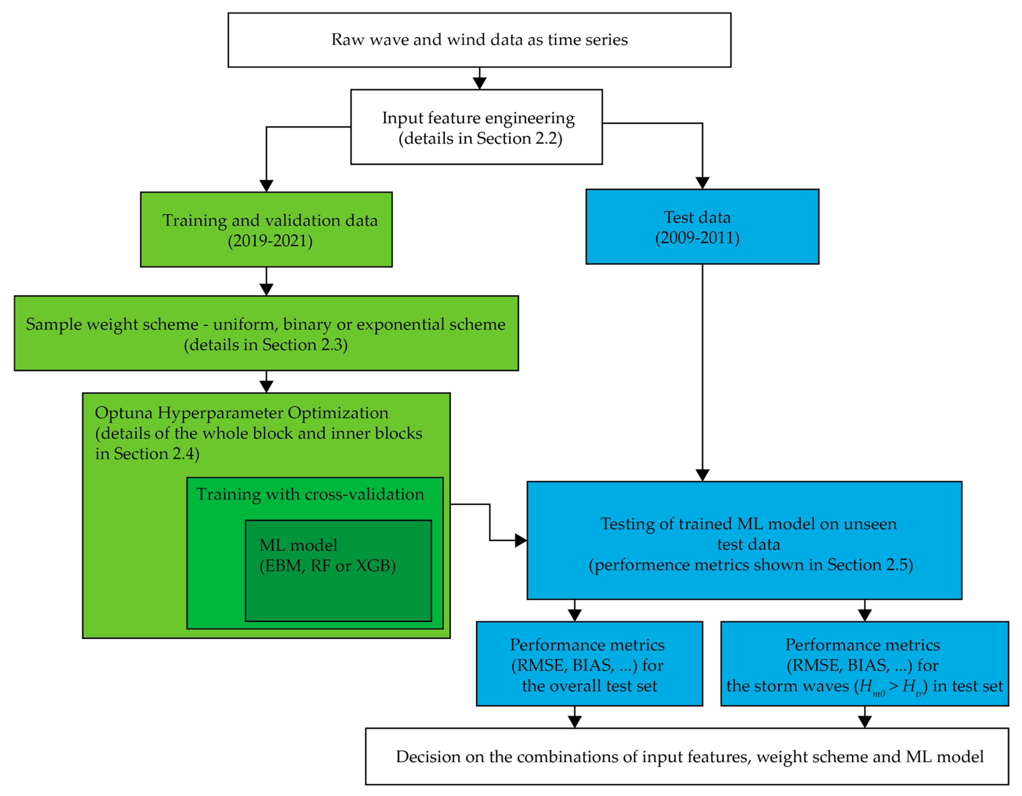
Figure 2 presents the complete workflow adopted in this study, moving from raw observations to final skill scores. At the top, we start with a continuous time series of buoy waves and land station wind measurements. Using the raw data, we create feature sets (the four different sets tested are described in Section 2.2.) that serve as inputs into the ML model, while H_m0 is always the model output. These data are split chronologically, where the green pathway on the left uses the recent 2019–2021 segment for model training with cross-validation, whereas the blue pathway on the right isolates the earlier 2009–2011 record for truly unseen testing (time series also visible in Figure 3).

Within the development branch, a user-selected sample-weight scheme—uniform, binary, or exponential (Section 2.3)—is first attached to the training/validation rows. The weighted data then enter an Optuna (version v4.4) hyperparameter search block, where each candidate setting of an Explainable Boosting Machine, Random Forest, or XGBoost model is trained with internal 5-fold cross-validation. The configuration that minimizes cross-validated RMSE is returned as the “best” model.

That trained model is next passed to the blue test branch, where it is evaluated on the untouched 2009–2011 observations. Two families of metrics, defined in Section 2.5, are reported, namely, overall statistics for every test hour and for storm wave conditions (H_m0 > H_tr). All test performance metrics are shown in

Table A1. Test matrix of different combinations of machine learning methods, input feature sets, weighting schemes, and their respective results on the test set 2009–2011 according to the performance metrics shown in Section 2.5.

N	ML Method	Feature Set	Weighting Scheme	RMSE (m)	BIAS (m)	R2	RMSE (m), Hm0 > Htr	BIAS (m), Hm0 > Htr
1	RF	Wind mag. and dir.	Uniform	0.100	−0.029	0.688	0.290	−0.199
2	RF	Wind mag. and dir.	Binary	0.103	0.008	0.668	0.240	−0.136
3	RF	Wind mag. and dir.	Exponential	0.104	−0.001	0.661	0.260	−0.042
4	XGB	Wind mag. and dir.	Uniform	0.101	−0.026	0.680	0.296	−0.201
5	XGB	Wind mag. and dir.	Binary	0.096	−0.012	0.708	0.264	−0.167
6	XGB	Wind mag. and dir.	Exponential	0.095	−0.007	0.715	0.255	−0.144
7	EBM	Wind mag. and dir.	Uniform	0.102	−0.032	0.670	0.294	−0.149
8	EBM	Wind mag. and dir.	Binary	0.105	−0.031	0.653	0.286	−0.128
9	EBM	Wind mag. and dir.	Exponential	0.127	−0.021	0.494	0.260	−0.107
10	RF	Wind components	Uniform	0.097	−0.027	0.701	0.290	−0.193
11	RF	Wind components	Binary	0.100	0.005	0.686	0.250	−0.131
12	RF	Wind components	Exponential	0.095	−0.002	0.715	0.240	−0.047
13	XGB	Wind components	Uniform	0.099	−0.025	0.691	0.296	−0.206
14	XGB	Wind components	Binary	0.095	−0.014	0.713	0.280	−0.200
15	XGB	Wind components	Exponential	0.091	−0.004	0.739	0.241	−0.139
16	EBM	Wind components	Uniform	0.099	−0.032	0.689	0.288	−0.206
17	EBM	Wind components	Binary	0.116	0.050	0.294	0.262	−0.164
18	EBM	Wind components	Exponential	0.122	0.092	0.531	0.250	−0.110
19	RF	Wind mag. and fetch	Uniform	0.098	−0.028	0.697	0.290	−0.192
20	RF	Wind mag. and fetch	Binary	0.099	0.003	0.693	0.240	−0.130
21	RF	Wind mag. and fetch	Exponential	0.100	−0.004	0.685	0.250	−0.046
22	XGB	Wind mag. and fetch	Uniform	0.100	−0.025	0.682	0.294	−0.189
23	XGB	Wind mag. and fetch	Binary	0.113	0.012	0.600	0.249	−0.150
24	XGB	Wind mag. and fetch	Exponential	0.095	−0.004	0.713	0.249	−0.138
25	EBM	Wind mag. and fetch	Uniform	0.104	−0.030	0.656	0.304	−0.127
26	EBM	Wind mag. and fetch	Binary	0.134	0.018	0.437	0.258	−0.154
27	EBM	Wind mag. and fetch	Exponential	0.120	−0.017	0.547	0.261	−0.103
28	RF	CEM-type inputs	Uniform	0.106	−0.023	0.645	0.300	−0.149
29	RF	CEM-type inputs	Binary	0.115	0.016	0.580	0.243	−0.079
30	RF	CEM-type inputs	Exponential	0.122	0.007	0.532	0.324	0.054
31	XGB	CEM-type inputs	Uniform	0.108	−0.019	0.630	0.310	−0.155
32	XGB	CEM-type inputs	Binary	0.127	0.032	0.489	0.259	−0.062
33	XGB	CEM-type inputs	Exponential	0.110	0.009	0.616	0.303	−0.045
34	EBM	CEM-type inputs	Uniform	0.107	−0.028	0.641	0.298	−0.143
35	EBM	CEM-type inputs	Binary	0.159	0.050	0.199	0.245	−0.076
36	EBM	CEM-type inputs	Exponential	0.136	0.015	0.412	0.298	−0.019

. Finally, a decision is made on which combination of input features, weight scheme, and ML model performs best.

We adopt a hindcasting approach to train a model on near-present observations of winds and waves to reproduce (hindcast) the wave heights from the given wind conditions in the past, rather than performing real-time forecasting. Specifically, we use the 2019–2021 subset for model training that includes a 5-fold cross-validation and then evaluate the trained model on the independent 2009–2011 subset, a strategy similar to that of previous studies. This split by time ensures that the model is truly predicting conditions it has not seen before, which is a stringent test of its hindcasting capability. The model skill is quantified by the standard error metrics shown in Section 2.5. on both the training and test sets.

We propose a data-driven hindcasting framework using three interpretable ML models—Random Forests (RF), Extreme Gradient Boosting (XGB), and Explainable Boosting Machine (EBM)—to predict hourly H_m0. We adopted these tree-based methods because they offer a deliberate progression in model complexity. EBM sits at the transparent end of the spectrum, as it fits a sum of one-dimensional step functions, so each predictor’s influence on H_m0 can be plotted directly and evaluated. Random Forests add one layer of sophistication by averaging hundreds of fully grown trees. This bagging captures higher-order interactions that an additive model may miss. XGB pushes the ensemble to its most expressive form by boosting trees sequentially, allowing the model to learn subtle residual patterns, while remaining explainable through gradient-based SHAP values and monotonic constraints. When considering the similarities between them, all three approaches inherit the core strengths of decision trees: they are non-parametric, require no a priori functional form, tolerate collinear and missing meteorological inputs, and accept per-sample weights—an essential feature for biasing the loss toward rare storm waves.

We expect that interpretability and generalization will trade off gradually along this hierarchy. Firstly, EBM should furnish the clearest physical insight but show the least predictive skill. RF should reduce bias and variance compared to EBM for most sea states, and XGB, while marginally more opaque, should deliver the lowest overall and extreme-wave errors. By analyzing all three, we obtain both a transparent diagnostic baseline and a performance ceiling, thereby demonstrating how much storm wave skill can be gained as the learning algorithm’s complexity increases while still retaining some post hoc explainability.

The methodology is designed to test different sets of input variables, as described in Section 2.2. Emphasis is placed on model interpretability and on strategies to improve performance for extreme waves (through sample weighting). This paper provides brief explanations of Random Forest (Section 2.4.1), Extreme Gradient Boosting (Section 2.4.2), and Explainable Boosting Machine (Section 2.4.3), with further details available in the cited references. All three ML models are implemented using open-source libraries (Scikit-learn [52], XGBoost [53] and InterpretML [54]). Hyperparameter tuning is performed via a Bayesian optimization with TPE (Tree-structured Parzen Estimator) implemented using the Optuna open-source optimization framework [55] on the training set (with internal 5-fold cross-validation). As demonstrated by Callens et al. [56], proper tuning (e.g., of tree depth, learning rates, etc.) can significantly improve model skill, so we automate this step. The final model configurations are chosen to maximize validation performance (e.g., lowest RMSE) while avoiding overfitting (monitored by performance on a validation set and compared to the test set).

2.4.1. Random Forest (RF)

Random Forest [57] is an ensemble of decision trees trained via bagging. Each tree in the forest is grown on a random subset of data and predictors, and the ensemble prediction is the average of all trees. RFs excel at capturing nonlinear interactions and typically have high accuracy and stability. They also provide measures of feature importance (based on a reduction in prediction error or impurity) which help interpret which inputs have the most influence on the output. Callens et al. [56] reported that RF could outperform neural nets in wave prediction performance. In our framework, RF serves as a robust baseline, and its partial dependence plots are used to verify physically sensible relationships (e.g., increasing H_m0 with higher wind speed).

2.4.2. Extreme Gradient Boosting (XGB)

Extreme Gradient Boosting is a gradient boosting tree model known for state-of-the-art predictive performance. Boosting builds an ensemble of shallow trees in sequence, where each new tree corrects errors of the previous ensemble (combination of all the previous trees). This typically yields higher accuracy than bagged forests, at the cost of a more complex model. XGBoost can also output feature importance and allows for post hoc interpretability analysis. In the wave prediction context, XGBoost has shown excellent results in [2], where it was shown that an XGBoost model gave the best overall performance for Lake Erie wave height and period hindcasts, beating a recurrent neural network in terms of error metrics. Similarly, our XGBoost model is expected to capture complex nonlinear links (like wind–wave interactions and fetch limitations) and serve as a high-accuracy benchmark. Technical details about gradient boosting trees can be found in [58].

2.4.3. Explainable Boosting Machine (EBM)

Explainable Boosting Machine is an interpretable Generalized Additive Model (GAM) enhanced with boosting [59,60]. The EBM fits a sum of feature-wise shape functions (and optionally some pairwise interaction terms) using cyclic gradient boosting. The result is a model of the form

H_m0 = f₁(feature1) + f₂(feature2) + … + c

where each f_i is a shape function learned from data but remains a simple function that can be plotted. We include EBM to prioritize interpretability—it provides transparent insights into how each input affects the prediction. The EBM is configured with moderate interaction terms (we allow the algorithm to discover 2–6 features that have a strong interaction) and a validation-based early stopping to prevent overfit. One advantage of EBM is that it could achieve accuracy comparable to black-box models while remaining a glass-box model [59,60]. By comparing EBM’s additive terms to known physical formulas (e.g., empirical wave growth laws), we can validate that the ML is learning sensible patterns.

2.5. Performance Metrics

After training each model with a given weighting scheme and input feature set, we evaluate performance on an independent test set obtained for the time period of 2009–2011. We report conventional regression metrics such as root mean square error (RMSE), mean absolute error (MAE), and coefficient of determination (R²) over the entire training and test set to gauge overall accuracy (Equations (7)–(10)):

$$\mathrm{RMSE}=\sqrt{{\displaystyle \frac{1}{n}}{\displaystyle \sum _{i=1}^n{(y_i-{\widehat{y}}_i)}^2}}$$

(7)

$$R^2=1-{\displaystyle \frac{{\displaystyle \sum _{i=1}^n{(y_i-{\widehat{y}}_i)}^2}}{{\displaystyle \sum _{i=1}^n{(y_i-\overline{y})}^2}}}$$

(8)

$$\mathrm{BIAS}={\displaystyle \frac{1}{n}}{\displaystyle \sum _{i=1}^n({\widehat{y}}_i-y_i)}$$

(9)

$$R={\displaystyle \frac{{\displaystyle \sum _{i=1}^n({\widehat{y}}_i-\overline{\widehat{y}})}(y_i-\overline{y})}{\sqrt{{\displaystyle \sum _{i=1}^n{({\widehat{y}}_i-\overline{\widehat{y}})}^2}{\displaystyle \sum _{i=1}^n{(y_i-\overline{y})}^2}}}}$$

(10)

where ${\widehat{y}}_i$ is the ith prediction, $y_i$ the ith observation, $\overline{y}$ is the average observation, and $\overline{\widehat{y}}$ is the average prediction. Special attention is given to assessing improvement in the high-wave regime (above storm threshold H_tr [50]). In the field of machine learning, assessing accuracy often involves the use of common performance metrics such as root mean squared error (RMSE) and BIAS, as referenced in [30,32,34,35]. To that end, we compute error statistics specifically for the upper tail of the distribution, such as RMSE and BIAS for H_m0 values above the 95th percentile of the test wave data. Ideally, a model with effective weighting will show minimal BIAS (no systematic underestimation) in this range. A key aspect of our evaluation is documenting the trade-off between overall accuracy and extreme-event accuracy. By construction, increasing the weight on extreme samples often improves error metrics for the high end at the cost of slightly worse performance at the low-to-moderate end [61]. An ideal outcome is one where extreme-wave errors drop significantly while the overall error increases only marginally.

3. Results

Section 3 evaluates hindcast skill in three stages. We begin in 3.1 by benchmarking the regional reanalysis models that serve as reference, MEDSEA [19] and COEXMED [44] (details about these models can be found in Section 2.1), against buoy observations to establish baseline error and bias in a fetch-limited setting. Section 3.2 then introduces our machine learning framework under a neutral (uniform) weighting scheme, examining how model choice and four alternative feature bundles influence overall accuracy relative to the reanalyses. Finally, Section 3.3 focuses on the upper five-percent tail of the wave height distribution, quantifying how well the same ML models with storm-specific weighting is applied reproduce storm peaks, which are an essential criterion for coastal design.

3.1. Comparison Between Measured Wave Data with MEDSEA and COEXMED Modeled Wave Data

Figure 4 compares the buoy measurements of significant wave height (H_m0) at Rijeka with two publicly available Mediterranean hindcast models. Panel (a) shows the comparison for the COEXMED model, while panel (b) presents the comparison for the MEDSEA model. Both datasets reproduce the overall variability reasonably well (R ≈ 0.82), yet the density clouds in the lower-left quadrant fall consistently above the 1:1 line, demonstrating a systematic negative BIAS for low-to-moderate sea states. Nevertheless, both products markedly underestimate the most energetic events, as many buoy peaks exceeding 2 m are below 1.3 m on the model axis, and the envelope of black storm points remain well above the 1:1 line (more on this in Section 3.3). Overall, this underprediction is 60% larger in COEXMED (−0.097 m) than in MEDSEA (−0.061 m), indicating that the MEDSEA reanalysis shows lower underprediction. The total scatter is also narrower in MEDSEA (RMSE = 0.133 m) than COEXMED (RMSE = 0.158 m).

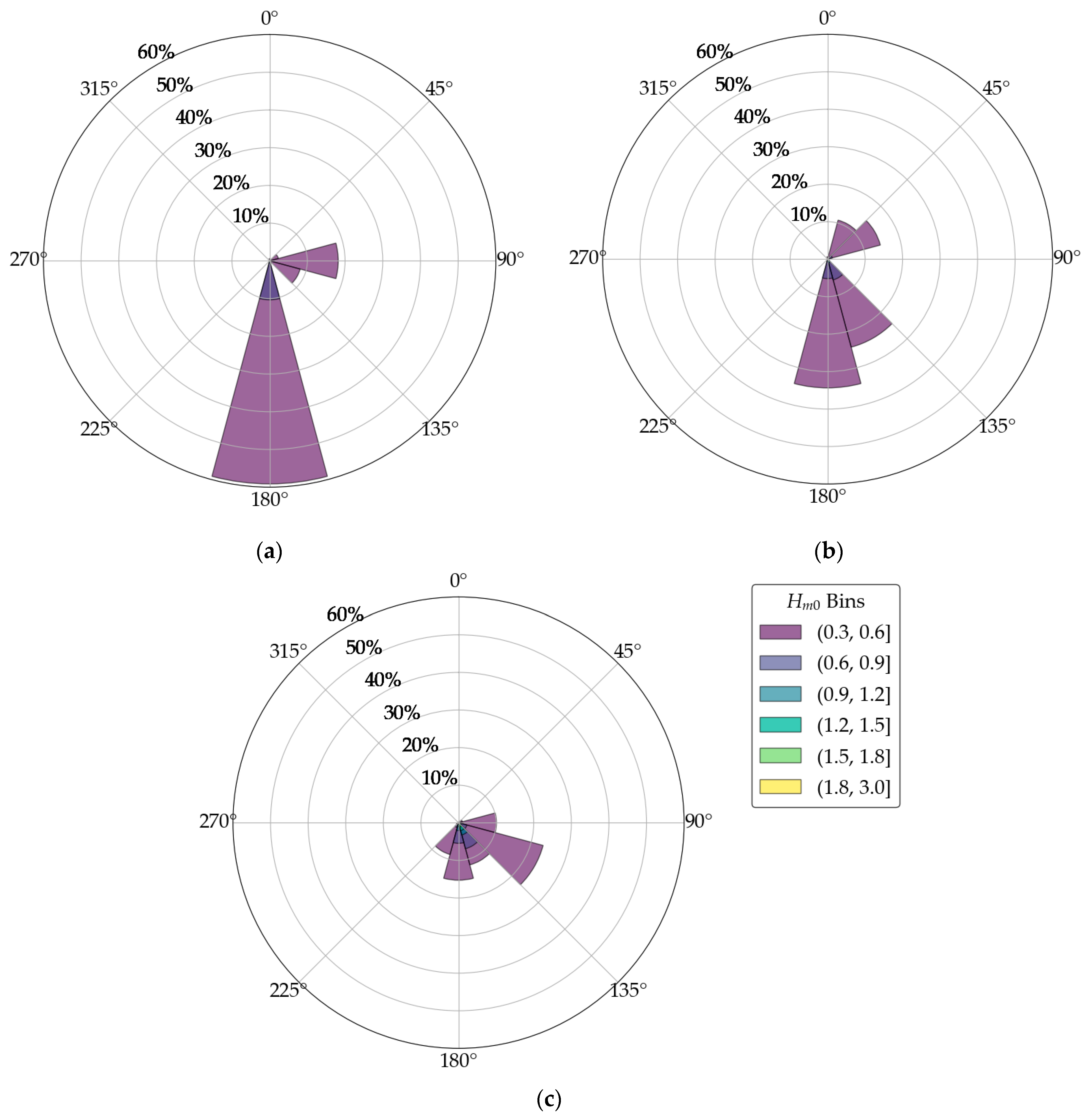
Figure 5 compares the directional wave-height climatology delivered by the two regional hindcasts to the buoy observations at Rijeka. Panel (a) shows the distribution simulated by COEXMED, panel (b) the corresponding distribution from the newer MEDSEA reanalysis, and panel (c) the wave roses derived from the measured series. In every polar diagram the azimuth indicates the direction from which waves travel, concentric circles give cumulative occurrence probability, and the wedge colors represent successive 0.3 m height classes, from 0.3–0.6 m (dark purple) up to 1.8–3.0 m (yellow).

The buoy data (panel c) show that more than two-thirds of all sea states arrive from the south-to-south–southeast sector (120–180°), where the Kvarner Gulf offers the longest uninterrupted fetch (Figure 1), while a secondary lobe centered near 90° records locally generated seas driven by episodic Bora (NE) winds. Importantly, every wave event exceeding about H_m0 = 1.2 m is confined to 135–185°.

COEXMED (panel a) reproduces the southerly dominance but collapses the spread into an unnaturally narrow beam around 180° and produces almost no energy in the southeastern quadrant. Because the model’s directional spread is too tight, high-wave counts are concentrated in a single direction, and the total frequency of low-to-moderate waves from 180° is overestimated (frequency of about 60%). MEDSEA (panel b) shows a slightly more accurate performance as it broadens the principal lobe toward 140–160°, so the overall shape resembles the observations more closely. Nevertheless, MEDSEA still under-represents the frequency of easterly waves, while showing a northeasterly wave direction, and shows too few storms from the acute SE sector around 90–130° that the buoy registers.

In summary, both MEDSEA and COEXMED reanalyses underestimate extreme waves in Rijeka’s fetch-limited setting, a limitation that motivates the site-specific, interpretable machine learning model shown in the subsequent sections (Section 3.2 and Section 3.3). Both hindcasts therefore capture the gross southerly control imposed by fetch geometry but remain unable to reproduce the full spread of storm wave directions.

3.2. Influence of Input Feature Preparation

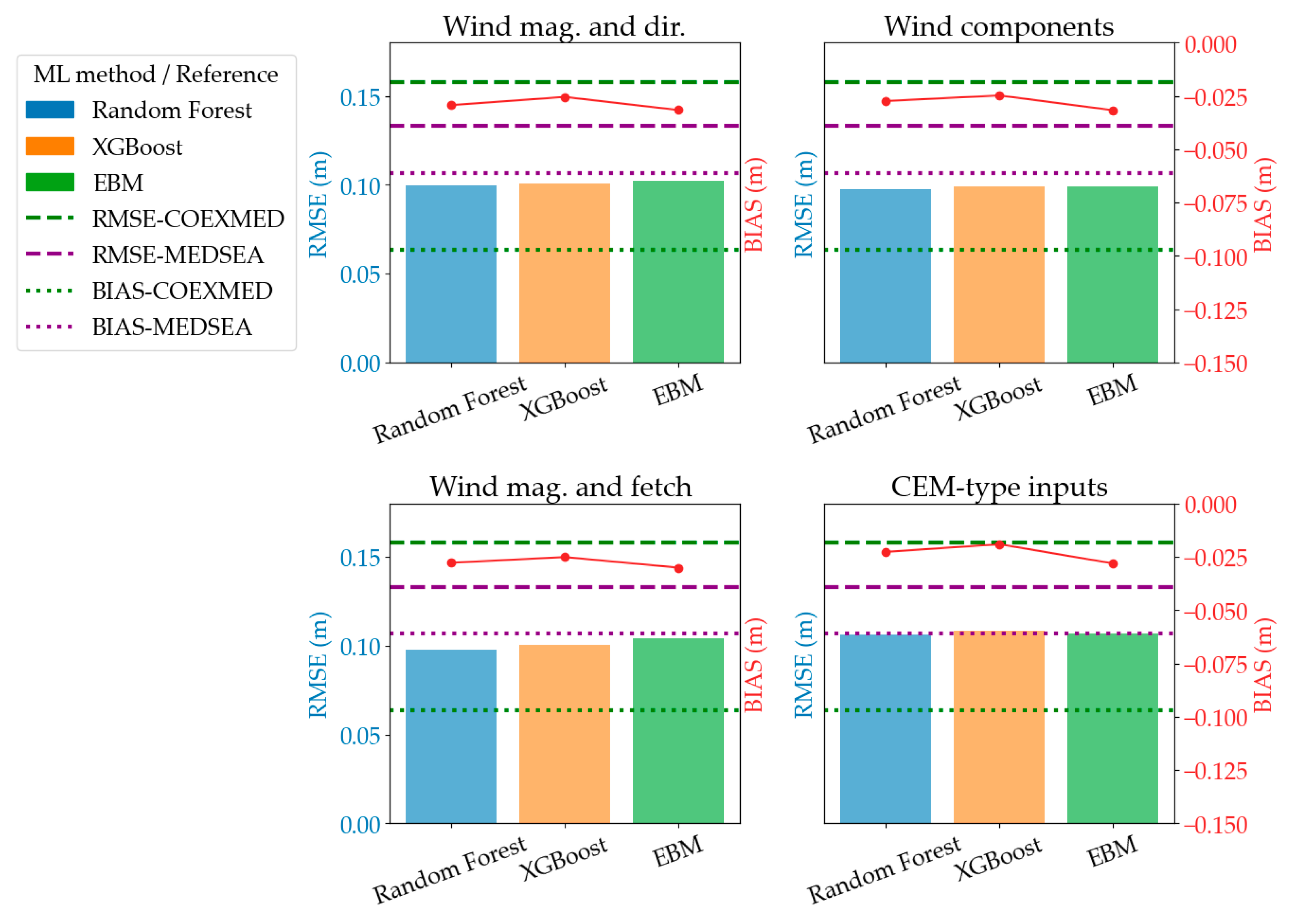
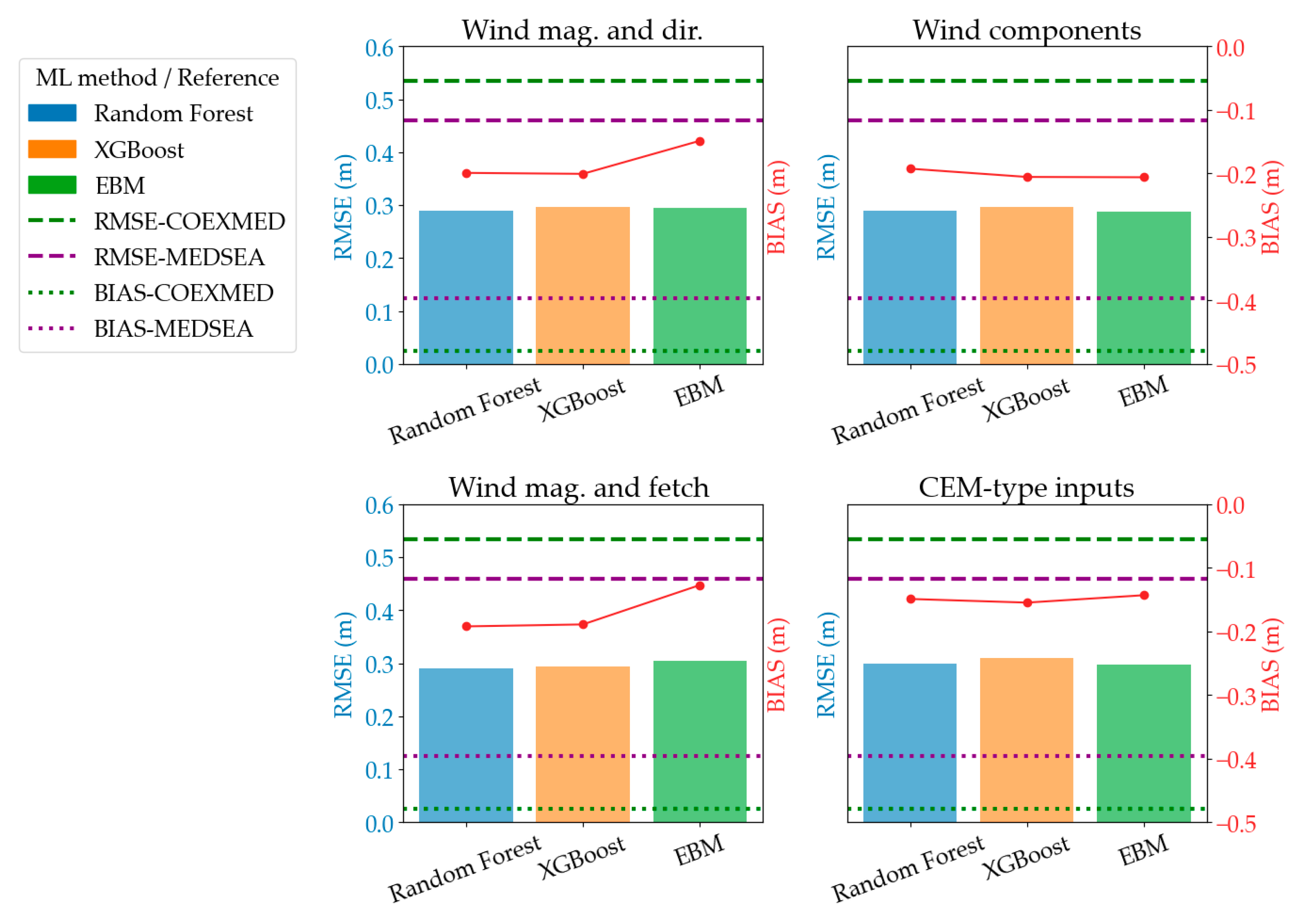
Figure 6 summarizes, for the uniform-weight experiments only, how four alternative feature bundles affect hindcast skill on the test set across the three tree-based algorithms. In every sub-panel, the colored bars show the overall RMSE obtained with Random Forest (blue), XGBoost (orange), and Explainable Boosting Machine (green); the red polyline traces the corresponding BIAS (right-hand axis). Horizontal dashed lines reproduce the error and BIAS levels of the regional hindcasts discussed earlier in Section 3.1—green for COEXMED and purple for MEDSEA—so that the ML models can be judged against these reanalysis models. In summary, the figure reveals that regardless of the specific machine learning model or feature engineering technique employed, the root mean squared error (RMSE) and BIAS values consistently fall within a 10% range, centering around an RMSE of approximately 0.1 m and a BIAS of approximately −0.25 m. Of critical importance is the clear demonstration that the performance metrics achieved by all the machine learning models and feature preparation methods detailed in this study are substantially better than those of the COEXMED and MEDSEA models, showing an improvement of roughly 25% from MEDSEA and 36%.

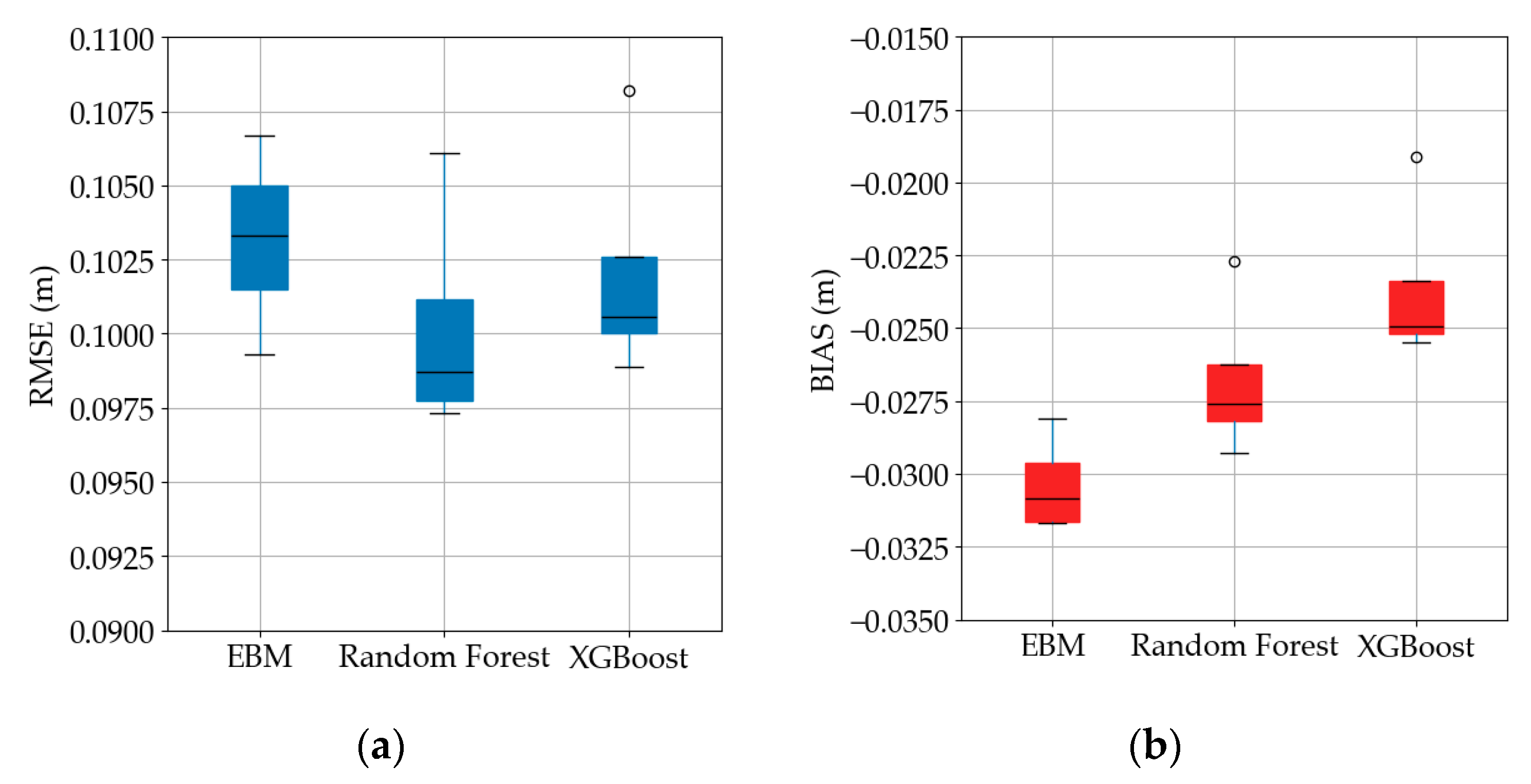
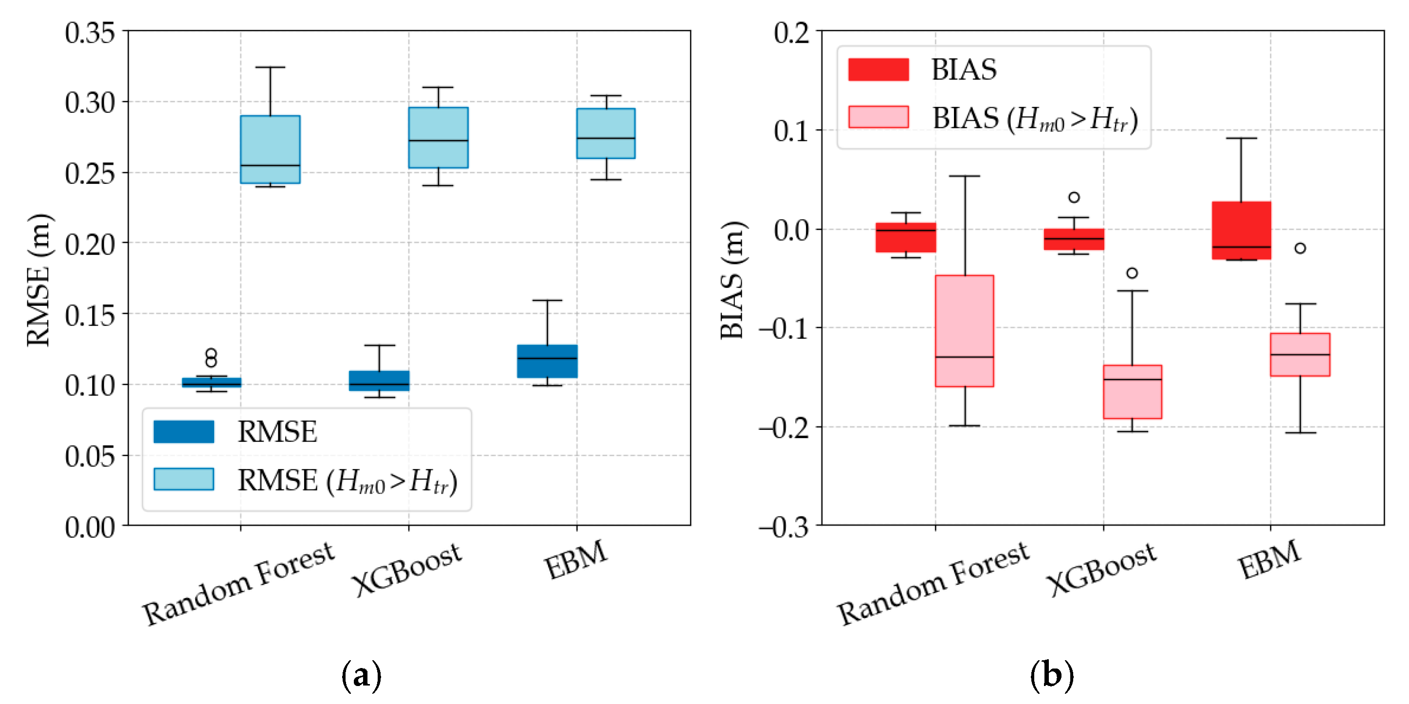
Figure 7 summarizes, with box-and-whisker statistics, the spread of overall error (left y-axis) and BIAS (right y-axis) obtained with the three learning algorithms regardless of feature set, while trained under a uniform weighting scheme. The Random Forest model exhibits the lowest and most stable error, with a median RMSE just at 0.980 m and an inter-quartile range of barely 0.003 m. XGBoost follows closely—its median is about 0.101 m and the central box is similarly tight, but one outlying fold reaches 0.108 m. The EBM shows the largest median value (≈0.103 m) and the widest inter-quartile span, indicating slightly higher and more variable residuals across the tests.

The BIAS distributions on Figure 7b confirm that all three models retain a small but systematic underprediction of significant wave height. Specifically, medians are clustered between −0.031 m and −0.025 m. EBM is the most negatively biased (median −0.031 m), Random Forest sits in the middle (≈−0.0275 m), and XGBoost is the least biased (≈−0.025 m). Taking together, the figure indicates that Random Forest and XGBoost offer comparable accuracy (RF for better RMSE, while XGB for better BIAS) for the present uniform-weight formulation. In this uniform weight scheme, EBM underperforms in both metrics.

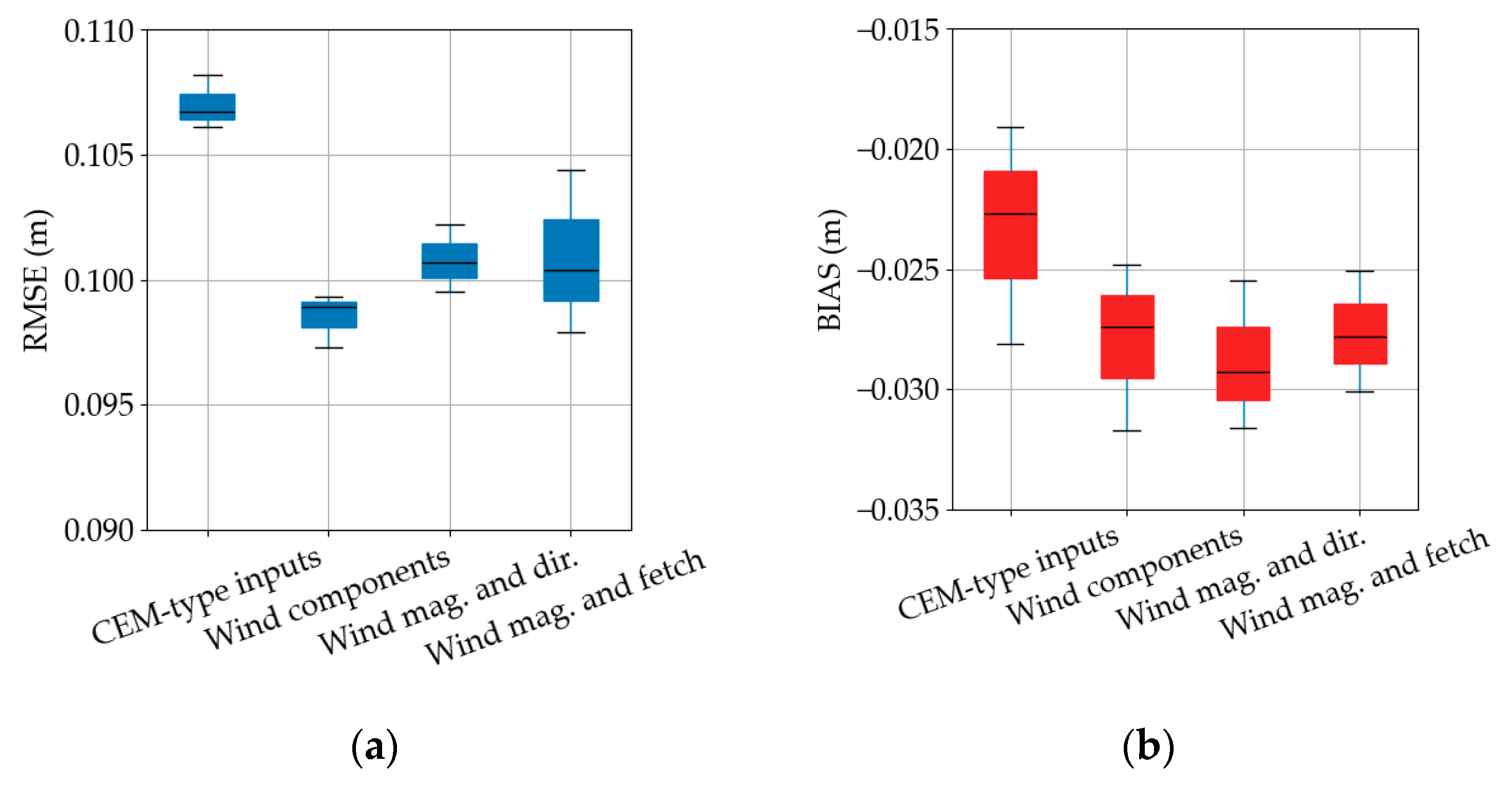
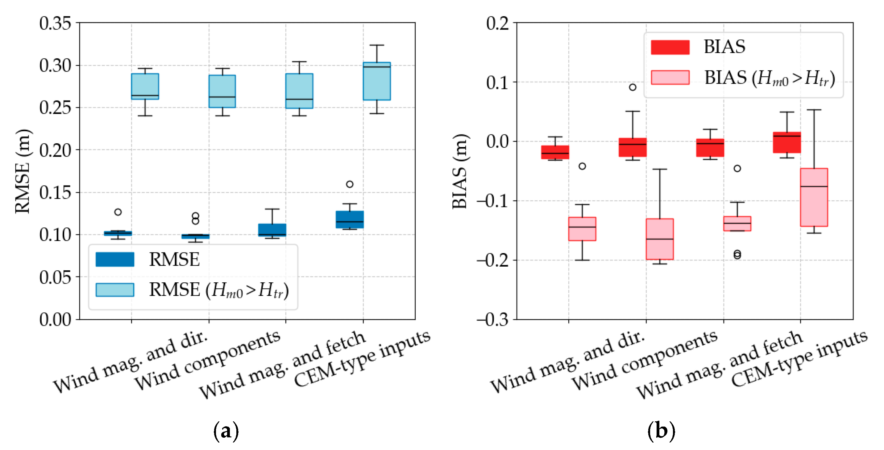
Figure 8 contrasts the predictive skill obtained with four alternative feature sets (described in Section 2.2.), with uniform weighting, regardless of ML model. The vector component formulation yields the lowest and most stable error, its median RMSE is just below 0.099 m, and the inter-quartile range is less than 0.0015 m. Both the magnitude-and-direction set and the magnitude-and-fetch set perform slightly worse (medians ≈ 0.101 m), with the fetch proxy also introducing greater variability. The CEM-type input set perform the worst, with a median RMSE of 0.107 m.

The BIAS values follow a similar pattern. All four formulations retain a small negative bias (underprediction), but the CEM-type feature set is best, with a median BIAS of −0.023 m. The other input feature sets show similar BIAS (medians ≈ 0.028 m).

Overall, the results show that the CEM-type feature set shows the lowest underprediction, while having the highest RMSE. On the other hand, converting wind speed and direction into continuous vector components shows improvement of 3% on the RMSE and 8% on BIAS.

3.3. Storm Wave Hindcast Accuracy

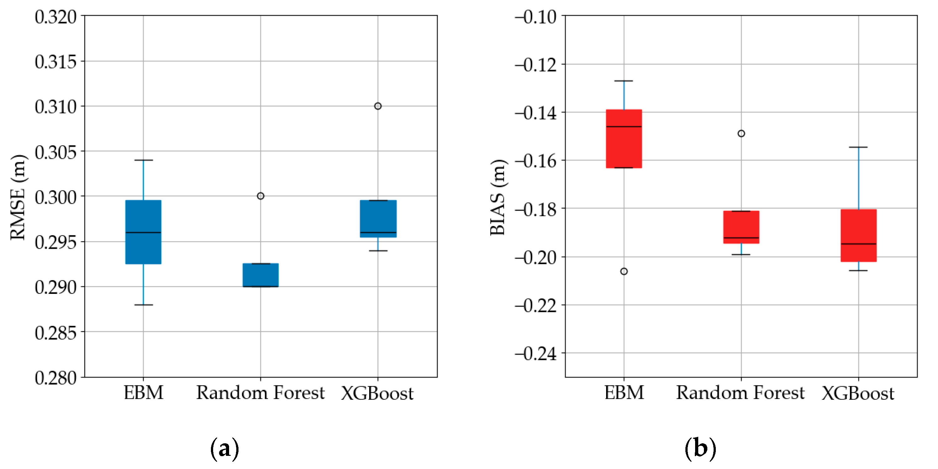
As described in Section 2.3., in this section, we analyze the performance metrics for storm waves (threshold is defined at H_tr = 95th quantile following [50]). Figure 9 presents how well each ML model reproduces the upper-tail sea states—those in the top five-percentile of the buoy record—under the uniform weighting scheme. Each sub-panel corresponds to one of the four feature bundles tested earlier. Within every panel, the colored bars display the tail RMSE of the three algorithms (Random Forest in blue, XGBoost in orange, and EBM in green). The horizontal dashed lines show the extreme-wave errors of the two reanalysis hindcasts (green = COEXMED, purple = MEDSEA) and their associated biases (green and purple dotted lines). Across all feature sets, every machine learning configuration outperforms the reanalysis by a wide margin. Specifically, tail RMSE falls at 0.53 m (COEXMED) and 0.46 m (MEDSEA) to the 0.25–0.35 m range, while the mean underprediction shrinks from about −0.39 (MEDSEA) and −0.46 m (COEXMED) to between −0.20 m and −0.27 m.

Figure 10 compares the three ML models when they are trained with uniform weights and evaluated only on the upper-five-percent tail of the wave-height distribution. Median RMSE remains near 0.30 m. Among the three algorithms, Random Forest performs best in this unweighted setting, its median RMSE lowering to ≈0.291 m and its spread confined to ±0.002 m. All models systematically underpredict storms, as shown in Figure 10b, with medians clustering between −0.14 m and −0.20 m. EBM is least negative (≈−0.15 m), while Random Forest and XGBoost show comparable BIAS at −0.19 m.

Figure 11 shows how the choice of input feature sets affects storm wave skill when the weighting scheme is kept uniform. The feature sets built from the orthogonal wind components performs best in terms of accuracy, its median extreme-wave RMSE lies at 0.29 m, and the inter-quartile range is narrower than 0.005 m. Adding fetch length data or using magnitude-and-direction set widens the error spread and raises the median to almost 0.295 m, whereas the purely empirical CEM-type composite parameters yield the poorest result, with median RMSE exceeding 0.30 m and a long upper whisker that reaches 0.31 m.

The CEM-type bundle shows the smallest underprediction (median ≈ −0.15 m) but pairs that virtue with the weakest RMSE. The wind component formulation, despite its superior RMSE, retains a slightly more negative BIAS (≈−0.21 m), though the distribution is tight. Both the magnitude feature sets yield intermediate performance, but they also exhibit broader BIAS ranges.

In combination, the panels confirm that converting wind direction to continuous vector components is essential for minimizing extreme-wave error but at the expense of higher underprediction, while relying on CEM-type parameters sacrifices accuracy even though it appears to reduce mean BIAS.

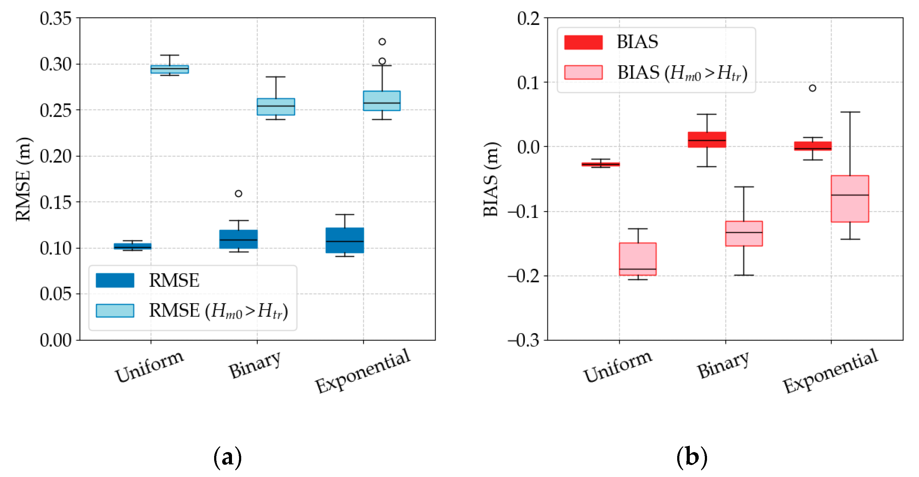
Figure 12 contrasts the three weighting strategies—uniform, binary, and exponential—across all ML methods and feature sets. The left panel plots box-and-whisker summaries of the overall RMSE (dark-blue bars) of the test set and, super-imposed in light blue, the RMSE calculated only for events exceeding the 95th-percentile threshold H_tr. The right panel shows the corresponding distributions of BIAS, with red boxes for the full test set and pink boxes for the storm wave subset.

With uniform weights, the model achieves the lowest median error on the full test set (≈0.10 m) but performs poorly on extremes. The storm-only RMSE is nearly triple the overall value, and the BIAS for large waves shows a strong underprediction of −0.17 m. Introducing binary weights—which assign extra weight to points above H_tr—decreases the extreme-wave RMSE down to ≈0.25 m and reduces 30% of the negative BIAS, while the overall BIAS becomes slightly positive. The exponential weighting scheme delivers the greatest improvement in tail accuracy. Specifically, its median storm RMSE falls to a comparable level as the binary scheme, but the BIAS reduces even further to ≈−0.07 m.

Figure 13 shows how the choice of predictor set influences hindcast skill when the model is trained across all weighting scheme and ML models. Most feature sets show similar performance metrics regarding extreme wave prediction accuracy, with only visible differences shown for CEM-type inputs, where, once more, RMSE (≈0.29 m) is sacrificed for an improved BIAS (≈−0.08 m).

Figure 14 contrasts the three ML algorithms across all feature sets and weight schemes. Random Forest yields the lowest RMSE for both overall and extreme conditions, and its median overall RMSE is just below 0.10 m, while the storm wave RMSE is at 0.25 m. XGBoost achieves a similar overall RMSE accuracy (≈0.10 m) but its tail error is higher (median ≈ 0.28 m). Explainable Boosting Machine lags behind, with its median storm wave RMSE clustering around 0.28 m, while overall RMSE is at 0.12 m.

All models retain some underprediction in the storm tail (≈−0.15 m), but Random Forest shows great variability with cases where the BIAS is completely diminished. Thus, Random Forest provides the most balanced performance—lowest and most stable RMSE together with the least BIAS—while XGBoost delivers comparable overall skill at the cost of greater storm wave underprediction, and EBM remains the least suited for heavily weighted storm prediction at this site.

Figure 15 presents density–scatter comparisons between buoy-measured significant wave height H_m0 and the values predicted by the best-performing ML model hindcast. The best-performing model is constructed using wind components as input features, using the Random Forest ML model and exponential weighting scheme. Appendix A Table A1, test case 12, details the performance metrics.

On the training set (Figure 15a), the cloud of points lies tightly along the 1 : 1 line from calm conditions up to about 1.6 m, with only a few isolated storm peaks (≈2.2 m) with slight underprediction. The summary statistics confirm the excellent fit, an RMSE of 0.067 m, a correlation coefficient R = 0.953, and a small positive BIAS of +0.022 m.

When the same model is applied to the test years (Figure 15b), skill remains high but naturally degrades. The point cloud is broader—especially at moderate heights—and several storm peaks are now underpredicted. Correspondingly the RMSE rises to 0.096 m and the correlation falls to R = 0.855, while the mean BIAS is at −0.006 m, revealing a slight underestimation. Even so, the test performance still surpasses that of the MEDSEA reanalysis by roughly 38% in RMSE and completely diminishes the overall BIAS, demonstrating that the model generalizes well across a decade-long gap. The storm wave metrics remain solid, with RMSE = 0.24 (50% decrease from MEDSEA) and BIAS = −0.047 (90% decrease from MEDSEA).

Figure 16 compares the measured evolution of significant wave height H_m0 during three representative winter storms inside the test data with the values produced by the regional hindcasts (COEXMED—blue; MEDSEA—red) and by the Random Forest model (green). Panel (a) covers the late-November 2009 storm sequence. Both regional products capture the timing of the three principal peaks but underestimate their amplitude throughout; the largest crest on 1 December reaches barely 0.9 m in COEXMED and 1.3 m in MEDSEA, whereas the buoy records 1.8 m. Random Forest reproduces the first two shorter storms almost exactly and tracks the third storm within ~0.4 m. Panel (b) shows a prolonged Sirocco episode in December 2009. Here, COEXMED severely damps the multi-day plateau, capping below 0.8 m, while MEDSEA reaches 1.0 m but still trails the buoy by ~1 m during the third storm. Random Forest traces the staircase-like growth pattern and maintains the elevated level for the correct duration, though it remains ∼0.5 m shy of the absolute maximum. Panel (c) portrays a storm on 20 February 2010 followed by two shorter fetch-limited bursts. Again, the reanalysis models lag behind as their main peak tops out at 0.7–0.8 m, whereas the buoy reaches 2.0 m. Random Forest attains 1.3 m—still an underprediction but a 60% reduction in peak error relative to MEDSEA—and captures both the timing and decay of the subsequent storms. Across the three cases, the Random Forest model consistently follows the observed phase and better approaches the true amplitude, particularly for rapid build-up and decay. COEXMED and MEDSEA reproduce the qualitative variability but underpredict considerably, underlining the benefit of site-specific, interpretable machine learning correction in a fetch-limited basin such as Rijeka Bay.

Figure 17 displays the permutation-based feature importances extracted from the best-performing Random Forest hindcast. Each bar quantifies the fractional increase in out-of-bag error that occurs when the corresponding predictor is randomly permuted, so taller bars denote variables that the model relies on most. The hierarchy is dominated by the meridional (V_y) wind component recorded at the Malinska wind station. The first-hour lag alone explains 17% of the model variance, the two- and three-hour lags add another 12% and 11%. The model therefore needs an accurate history of V_y over the past three hours to estimate how far wave growth has progressed. The instantaneous V_y measured near the buoy site (Rijeka) ranks fourth, showing that local winds refine but do not replace the broader-scale forcing captured by the Malinska station. In contrast, zonal components (V_x)—which distinguish eastward from westward winds—appear lower in the list and drop steeply beyond the third lag component. Below the top fifteen, further lags of both V_x and V_y at either station carry negligible weight. The importance profile corroborates a physically intuitive picture, in which significant wave height at Rijeka is governed primarily by the recent history of the south–north wind, with diminishing returns from older or east–west wind information.

4. Discussion

This work presents results demonstrating that a locally trained, interpretable machine learning hindcast model surpasses the performance of two established Mediterranean reanalysis datasets at a fetch-limited location, achieving a practically and statistically significant improvement in accuracy. When considering the model that showed best performance across all metrics (test number 12 in Table A1), we used the training dataset in the timeframe of 2019–2021 for a Random Forest (RF) model using only onshore wind vector components and an exponentially weighted upper tail of the wave height distribution. To test the accuracy of this model (and other tested models in Table A1), we used data 10 years prior to the training data (2009–2011) to rigorously test the hindcast accuracy of the model. On the training data, the RF model (test number 12) achieved a root mean square error of 0.067 m, a Pearson correlation of 0.953, and a negligible mean BIAS of +0.022 m. Testing the RF model on unseen 2009–2011 data increased the RMSE to 0.096 m and reduced the correlation to 0.855; however, the forecast remained superior to COEXMED and MEDSEA, which had RMSE errors of 0.14–0.16 m. Figure 15’s density–scatter diagrams show that the RF model closely tracks the one-to-one line across most data points, deviating only significantly at the highest peaks where observational uncertainties and few training examples increase scatter. Despite this, the RF prediction time series still tracks the phase of each event, in contrast to the regional products which show flattened peaks (Figure 16).

These quantitative gains are not outliers when viewed against the broader literature. The authors of [7] reported a 29% reduction in normalized RMSE after applying a multi-layer perceptron (ANN) to bias-correct a MEDSEA hindcast. Even though our improvement on the overall test dataset is slightly larger in absolute terms (reducing RMSE from 0.133 m for MEDSEA to 0.096 m for the RF), it is notable that this was achieved without a numerical model wave prediction as an input feature and uses an interpretable architecture allowing for inspection of individual feature effects. Further research by Hu et al. [2] revealed that an XGBoost model, utilizing open-lake buoy data from Lake Erie for training, produced correlation coefficients ranging from 0.95 to 0.97 and a MAPE between 15.6% and 22.89%. This study did not achieve the same accuracy, in part due to the input data. Hu et al.’s study utilized fifteen years of wind data from an offshore buoy (the same used for wave data), unlike our own data collected at the Rijeka wind station, which is located at 120 m a.s.l. in an area of exceptionally steep terrain. In contrast, the authors note that their basin’s practically boundless fetch makes it easier to model than the confined inlets we examined. Achieving a correlation of 0.855 and a mean absolute percentage error (MAPE) of 45% on the test set indicates comparable performance in a more geometrically challenging setting. However, concerning storm wave performance, Hu et al.’s ML models exhibited a normalized BIAS ranging from −3% to −10%, which is larger than the −1.3% BIAS of our study’s best-performing RF model. Abdelhady et al. [62] showed a machine learning framework, using land-based wind data and incorporated a complex ConvLSTM-1D ensemble to predict wave buoy measurements on the Great Lakes near Chicago. Despite its simplicity (only two wind stations and RF modeling), our model’s results are comparable to those of the more complex four-wind-station model, differing by less than 10% in RMSE and BIAS.

A significant contribution of this study is the systematic investigation of various weighting schemes. As illustrated in Figure 12, the prevalence of calm seas over storms in the dataset leads to an underestimation of the highest waves by roughly 0.17 m across all algorithms using uniform mean square loss. Using a binary weighting scheme (800 for observations above the 95th quantile) decreases underprediction to −0.13 m; however, the overall RMSE increases by 10%, and BIAS variability becomes larger. Using exponential weighting reduces the storm BIAS to −0.07 m, without negatively impacting other metrics compared to the binary method. Therefore, the binary scheme is the least useful option; however, if storm waves are truly significant, the exponential scheme should be selected, and if general climate conditions are important, a uniform scheme is most appropriate.

The analysis reveals that representing wind direction using continuous sine–cosine components, rather than the original directional numeric values, significantly improved the model accuracy; this is evidenced by a 3% decrease in the overall RMSE, a 2% reduction in storm wave RMSE (Figure 8 and Figure 11 illustrate these improvements), and an 8% decrease in overall underprediction. In contrast to the measurable benefits provided by vector component sets, incorporating a numeric variable that can effectively fetch data does not offer any discernible improvement or advantage. However, it is noteworthy that while CEM-type input features yield the worst RMSE scores of any feature set tested, they also achieve the lowest degree of underprediction in both the overall test set and the more specific subset of data focused exclusively on storm waves. Upon conducting a feature importance analysis on the top-performing Random Forest model, the results clearly demonstrate the dominance of meridional wind readings obtained from the more distant mainland weather station (Malinska wind station) as the most influential factors. The most prominent are the three-hour period before a buoy ‘current’ observation (in other words, the three lag V_y components observed in Malinska wind station), a fact which supports the idea that wave memory rarely surpasses the theoretical time needed for growth with a 30 km fetch and winds of about 10 m per second (CEM equations show that wave saturation in this area is around three hours). While the research conducted by Abdelhady et al. [62] indicates that incorporating data from extra wind stations into our machine learning model could significantly improve its performance, with up to a four-wind-station integration showing a substantial boost, the current lack of accessibility of this type of data for the Rijeka Bay unfortunately prevents us from implementing this improvement.

Among the tested ML approaches, Explainable Boosting Machine (EBM) stands out as a particularly interesting option due to its high level of explainability, a characteristic that earns it the designation of a glass-box model. Compared to the more complex and capable RF and XGB models, it performed significantly worse, failing to capture the intricate relationships between input and output. However, for storm waves, the EBM model showed a comparable RMSE to the other two models, and even a 25% lower rate of underprediction (BIAS = −0.14 m for EBM, and BIAS ∼ −0.19 m for RF and XGB in Figure 10), making the EBM still an interesting choice for storm wave prediction when no weight schemes are used. Like XGB, the EBM model performed poorly with sample weighting. For this reason, due to a better response of RF models to incorporate sample weights and focus on storm wave accuracy, we prefer RF (test number 12 in Table A1) with exponential weight schemes opposed to XGB (test number 15 in Table A1) with the same weight scheme. Test 12 showed 67% lower BIAS and similar RMSE for storm wave situations, while sacrificing 3% in overall R² and 5% in overall RMSE.

5. Conclusions

This study set out to determine whether an interpretable, data-driven hindcast can equal or surpass the skill of state-of-the-art regional wave products in a fetch-limited Mediterranean bay while preserving a clear link to physical understanding. Using only hourly wind observations from two on-land stations and a wave buoy in Rijeka Bay, we trained and compared three tree-based algorithms—Random Forest (RF), XGBoost (XGB), and Explainable Boosting Machine (EBM)—under three loss-weighting schemes and four input feature sets as a feature engineering effort.

Two findings stand out when tested on an unseen test set 2009–2011 period. First, recasting wind direction into continuous sine–cosine components (feature set 2 in Table 2) decreased both RMSE and BIAS, while proving to be the most reliable feature set. Second, explicitly weighting the loss toward large waves changed the hierarchy of models and sharply improved storm performance. Uniform weighting left models with a BIAS mainly between −0.14 m and −0.19 m (underprediction) for the top five-percent waves; an exponential weighting lowered that BIAS to −0.07 m and cut the tail RMSE to ≈0.25 m without significantly inflating the overall RMSE.

The best RF model achieved an RMSE of 0.096 m and a correlation of 0.855 (Table A1, test number 12)—approximately a one-third overall RMSE reduction relative to MEDSEA and COEXMED, while for storm wave data, the RMSE decreased by 50% and BIAS underprediction by 90% relative to MEDSEA [21] and COEXMED [46]. It is worth noting that MEDSEA and COEXMED are state-of-the-art regional wave reanalysis models. Time series comparisons for three winter storms confirmed that the RF hindcast tracks both the phase and amplitude of multi-peak events far more closely than either reanalysis models, trimming peak error by up to 60%. These improvements resulted from a model that offers real-time performance, trains rapidly within an hour, and provides transparency into each predictor’s impact. These quick and responsive tools, such as the RF model with sample weights, has a significantly higher accuracy and lower computational costs than a commonly used reanalysis wave models.

To meet growing regulatory demands for confidence intervals, future research could explore probabilistic approaches such as quantile regression forests and conformal prediction; this is vital for effective harbor management. Also, using regional downscaling or MEDSEA wave reanalysis with a local RF model and other ML models in an ensemble approach could create a fast and efficient operational system. This could significantly improve the accuracy of wave prediction for a relatively low computational cost.