Abstract
Inverting seawater sound speed profiles (SSPs) using Bayesian methods enables optimal parameter estimation and provides a quantitative assessment of uncertainty by analyzing the posterior distribution of target parameters. However, in nonlinear geophysical inversion problems like acoustic tomography, calculating the posterior distribution remains challenging. In this study, a Bayesian framework is used to construct the posterior distribution of target parameters based on acoustic travel-time data and prior information. A Hamiltonian Monte Carlo (HMC) approach is developed for SSP inversion, offering an effective solution to the computational issues associated with complex posterior distributions. The HMC algorithm has a strong physical basis in exploring distributions, allowing for accurate characterization of physical correlations among target parameters. It also achieves sufficient sampling of heavy-tailed probabilities, enabling a thorough analysis of the target distribution characteristics and overcoming the low efficiency often seen in traditional methods. The SSP dataset was created using temperature–salinity profile data from the Hybrid Coordinate Ocean Model (HYCOM) and empirical formulas for SSP. Experiments with acoustic propagation time data from the Kuroshio Extension System Study (KESS) confirmed the feasibility of the HMC method in SSP inversion.
1. Introduction
The sound speed profile (SSP) characterizes the variation law of wave propagation speed with depth, and serves as the basis for achieving accurate acoustic detection. Its precision determines the application effectiveness of marine acoustic technologies in sonar detection [1,2,3], marine environment monitoring [4,5,6], and seabed topographic exploration [7,8].
Since seawater temperature and salinity are influenced by factors like sunlight and precipitation, the SSP exhibits significant spatiotemporal variability. These features make large-scale and long-term measurements of the SSP using instruments very challenging [9,10,11]. In the 1970s, Munk and Wunsch introduced the concept of ocean acoustic tomography. They explained the fundamentals of forward problems, inverse problems, and observation technologies. They successfully derived the SSP by analyzing the travel time of acoustic waves over long distances in the ocean, which laid the foundation for SSP inversion [12]. SSP inversion involves estimating key parameters of the SSP from observed data like acoustic wave travel times. Compared to methods that directly measure the SSP with instruments, inversion techniques more effectively address the limitations faced in large-scale surveys [13].
From matched-field inversion techniques developed in the 1990s to recent advances in deep learning-based inversion, SSP inversion methods have consistently addressed challenges related to spatiotemporal resolution and dynamic response [14,15]. Scholars like Tolstoy and Skarsoulis introduced various SSP inversion approaches based on time reversal around the 1990s, including matched-field inversion and peak-matching of the theoretical sound field with the measured sound field. However, issues such as environmental parameter mismatch, statistical noise interference, and systematic model deviations remain prominent, which can easily lead to problems such as the non-uniqueness of inversion results or distorted evaluations [16,17]. In SSP inversion research, as depth increases, the number of parameters required during the inversion process rises significantly, and the demands for inversion accuracy also increase. This makes solving the inverse problem more difficult and nonlinear [18]. LeBlanc et al. proposed a method to represent SSP using Empirical Orthogonal Functions (EOFs). EOFs can characterize the main spatiotemporal variations of SSP with only the first few modes, reducing the number of parameters needed for SSP inversion and lowering the process’s complexity. This provides a feasible way to transform the SSP inversion problem into an optimization problem [19]. Inversion techniques combined with EOF decomposition remain the primary methods for SSP inversion at present [20,21].
Since the beginning of the 21st century, many scholars have integrated Bayesian concepts, heuristic algorithms, and deep learning methods into SSP inversion. This has significantly enhanced the ability to track changes in SSP characteristics and increased inversion efficiency, providing a strong technical foundation for future data-driven methods [22,23,24,25]. When using optimization algorithms for SSP inversion, traditional gradient-based techniques iteratively adjust parameters to minimize the objective function. These methods work well for low-dimensional parameter inversion but often become trapped in local optima in high-dimensional SSP inversion [26]. The probabilistic search of the simulated annealing algorithm helps alleviate the problem of local optima. However, its overall convergence is usually slow, and computational costs increase sharply as the parameter space expands [13]. With advances in data science, data-driven strategies have grown increasingly important for SSP inversion, with deep learning algorithms showing impressive performance. These methods can establish nonlinear mappings between acoustic field features, environmental parameters, and SSP without relying on complex physical models, enabling rapid inversion. However, they require large amounts of high-quality training data. Due to the complexity of the marine environment, collecting measured data faces challenges such as high costs and limited acquisition scope. Consequently, deep learning algorithms find it difficult to learn the complex laws governing the marine environment solely from high-quality training data, which significantly limits their ability to generalize [27,28].
Inversion methods based on a specific optimization criterion often provide only a single parameter solution, which frequently overlooks uncertainties caused by noise, errors in observed data, and prior information. Bayesian inversion introduces a new approach for quantifying uncertainties in the SSP inversion problem. Unlike traditional methods, Bayesian inversion examines the posterior distribution of parameters using its moments, providing not only optimal parameter estimates but also a quantitative assessment of the confidence level in the inversion results [29,30,31,32]. In nonlinear geophysical inversion problems like acoustic tomography, a key challenge of Bayesian inversion is the numerical calculation of the posterior distribution. The development of the Markov Chain Monte Carlo (MCMC) algorithm has offered an effective solution to this challenge [33,34,35,36,37].
Based on the Bayesian inversion framework, this paper introduces a method for inverting seawater SSP using the Hamiltonian Monte Carlo (HMC) algorithm. The proposed method has significant research implications: 1. The inversion solution derived from this approach does not yield a single value but instead provides the posterior distribution of the target being inverted. 2. This paper demonstrates the feasibility of using the HMC algorithm to explore the complex distributions of unknown SSP parameters and ultimately enables analysis of the inversion results and their uncertainties through statistical moments. 3. It also discusses the advantages and disadvantages of the HMC algorithm in SSP inversion, offering valuable guidance for future research.
The rest of the paper is organized as follows: Section 2 mainly discusses the forward model of SSP, the solution to the SSP inverse problem, and the HMC algorithm. Section 3 focuses on applying the proposed method to measured data and analyzing the results. Finally, Section 4 offers conclusions and recommendations.
2. Methods
2.1. Forward Model
A forward model is a deterministic system that predicts experimental observations d using theories or physical laws based on known parameters m. In the inversion of SSP, the observation d is the round-trip propagation time, and the model parameter m is the sound speed parameter to be estimated. The forward model explains how to calculate the total round-trip acoustic propagation time with known sound speeds, where the following equation defines the total acoustic propagation time :
where represents the total round-trip time of the acoustic wave in the vertical direction from the sea surface to the instrument’s position, is the initial position of acoustic wave emission, is the depth of the receiving point, denotes the sound speed variation with depth z, i.e., SSP, and is the error term.
As the depth of seawater increases, the number of parameters αₖ to be inverted for the SSP grows nonlinearly. This paper reduces the required number of parameters by decomposing a single SSP using EOF:
where represents the average sound speed in the target region. and are the Empirical Orthogonal Function (EOF) coefficients and the Empirical Orthogonal Function of the SSP, among which is reconstructed via the least squares method.
By interpolating the N SSPs in the target region at equal intervals into M vertical standard layers to form a sound speed matrix, the covariance matrix can be defined by the following equation:
Here, is the perturbation matrix, where . The average sound speed matrix can be defined by the following equation:
where is the discretized representation of the continuous sound speed function , and is the index of the discrete nodes, . After performing EOF decomposition on the covariance matrix in Equation (3), the eigenvalues and eigenvectors can be obtained. Arrange the eigenvalues in descending order. Then, the eigenvectors corresponding to the first -order eigenvalues can be selected to represent the SSP.
Using Formula (2), we transform the problem of inverting a single SSP into the problem of inverting the first k-order EOF coefficients. At this point, the model parameter to invert is m, which equals the vector , where the cumulative contribution rate of the first k-order EOF eigenvalues is represented as
where quantifies the explanatory power of the first k-order EOF components for the original data. It is generally considered that if is greater than 95%, the explanatory power is sufficient [38].
2.2. Solution to the SSP Inverse Problem Under Bayesian Inference
Within the Bayesian framework, the solution to the seawater SSP inverse problem is not a single definitive value but a posterior distribution that combines observational data and prior knowledge [31,37]. As shown by Bayes’ theorem, the conditional distribution of the model parameter m given the observational data d is expressed by Bayes’ theorem as follows:
Here, represents the posterior distribution of the model parameter m given the observational data d. The conditional distribution embodies the relationship between observational variables and model parameters, and is our existing knowledge about the model parameter before obtaining the observational data. is a normalization constant and is independent of the model parameter m. Thus, Equation (6) can be written as follows:
In the SSP inversion problem, our goal is to invert the SSP parameters using the total round-trip time of acoustic wave propagation. Thus, in Equation (7), the observed variable d can be replaced with the observation vector of acoustic propagation time. Given the observation vector , the conditional distribution is numerically equal to the likelihood function , and the posterior probability density can be expressed as the following equation:
The likelihood function represents the level of support that observational data provide for model parameters. In measuring acoustic propagation time data, noise is often not an ideal Gaussian distribution but shows heavy-tailed characteristics. We assume that the observation time error follows a Laplace distribution, whose tails decay more slowly than those of the Gaussian distribution and thus can better match the actual observational data’s characteristics. The likelihood function can be expressed as the following equation:
where is a scale parameter that controls the degree of dispersion of time errors. In general, it is set equal to the data error. represents the time difference, where , and denotes the theoretical propagation time calculated by the forward model of the SSP.
Ultimately, based on the observed variables, the posterior distribution of the model parameter m can be expressed as
In SSP inversion, this paper assumes that the prior distribution is a uniform distribution. Equation (10) provides the solution to the SSP inverse problem; however, due to the complexity of nonlinear problems, the posterior distribution in Equation (10) is difficult to solve directly through an analytical approach. Therefore, we turn to numerical methods to compute the posterior distribution of the model parameter m.
2.3. Hamiltonian Monte Carlo
The MCMC algorithm samples by constructing a Markov chain that converges to the posterior distribution. This method does not require knowing the exact form of the target distribution, and the main features of the distribution can be understood from the statistical properties of the samples. When sampling complex posterior distributions, traditional MCMC algorithms often have difficulty efficiently exploring the distribution structure due to low efficiency [39]. To improve the performance of traditional MCMC algorithms in complex distributions, Duane proposed the HMC algorithm, which combines classical Hamiltonian mechanics. By using gradient information to enable “directed leaps” during sampling, it greatly enhances exploration efficiency in complex distributions and offers a new approach for exploring such distributions [35,36].
Figure 1 illustrates the sampling trajectories of the Metropolis–Hastings (M-H), Gibbs, and HMC algorithms in a two-dimensional Gaussian distribution. Starting from the same initial point [4.8245, 5.4051], the number of steps is 25, the HMC algorithm is the first to reach the high-probability sampling region, and it also has a higher acceptance rate than the M-H and Gibbs algorithms.
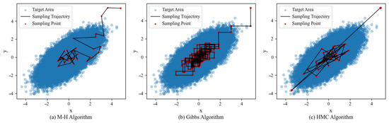
Figure 1.
Sampling trajectories of three MCMC algorithms in a two-dimensional Gaussian distribution . (a) Sampling trajectory of the M-H algorithm; (b) sampling trajectory of the Gibbs sampler; (c) sampling trajectory of the HMC algorithm.
The main idea of HMC is to turn the sampling problem into an evolution process of a dynamic system by using dynamic simulations in physical systems. HMC considers the target model parameter m as the position of a particle, and the potential energy function U(m) of the particle is defined as the negative logarithm of the target posterior distribution :
For the inverse problem of the SSP, the target posterior distribution is defined by Equation (10).
It is usually necessary to artificially introduce a momentum variable p to form a complete Hamiltonian system, where the kinetic energy K(p) is defined as
Here, M represents a mass matrix. Generally, we utilize a quadratic form of kinetic energy [36,40].
The total Hamiltonian energy of the system is determined by both the potential energy and the kinetic energy:
The total Hamiltonian energy remains constant during the system’s evolution, and the system evolves according to Hamiltonian’s equations:
Here, represents the integration time. The HMC algorithm updates the position and momentum by integrating Equation (14) over time.
In practice, the HMC algorithm utilizes the gradient information of the target distribution for momentum updates, and typically employs the Leapfrog method to simulate the updates of particle positions and kinetic energy. Let represent the step size of particle motion; then, the position m and momentum p of the particle are updated according to the following equations:
The trajectory of particle motion simulated using the Leapfrog method is constructed based on the geometric structure of the target distribution. Consequently, it enables directed exploration, thereby effectively reducing the inefficiency incurred by the random walk behavior inherent in traditional MCMC algorithms.
When simulating the particle trajectory with the Leapfrog method, the process will generate some errors due to time discretization. Therefore, it is necessary to include a rejection–acceptance step for correction.
Here, represents the new state obtained after simulating L steps of Hamiltonian mechanics with a step size of starting from the initial state . This state is accepted as the next state with the probability given in Formula (16); if the proposed state is not accepted, the next state remains the same as the current state.
The pseudocode for the HMC algorithm is shown in Appendix A. The HMC algorithm, based on classical Hamiltonian mechanics and incorporating the Metropolis correction, constructs a phase space that includes position and momentum variables. It moves through this phase space using information from the target posterior distribution, ultimately disregarding the momentum to generate samples from the model parameters’ posterior distribution. With enough runtime, the sample mean will approach the expected value.
3. Experiments and Results Analysis
3.1. Experimental Data
3.1.1. Acoustic Propagation Time Data
The acoustic propagation time data used in the experiments of this paper are derived from the Kuroshio Extension System Study (KESS) (https://www.po.gso.uri.edu/dynamics/KESS/CPIES_data.html, accessed on 18 July 2025). This study focuses on the East Sea of Japan as the survey area, with the specific scope defined as 28.5–39° N, 141–148° E. A total of 46 PIES instruments were deployed in the measured sea area. The study area (shown as the blue area in the left panel) and the deployment locations of the PIES instruments are displayed in Figure 2.
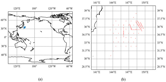
Figure 2.
Map of the study area and diagram showing instrument deployment. (a) Map of the study area, with the blue area representing the study zone; (b) diagram illustrating instrument deployment, with the red dots indicating the locations of PIES instruments.
The experimental data on the total round-trip sound propagation time selected in this paper were collected by instruments deployed at two different locations in 2005, with instrument numbers H6_SN166 and C6_SN173. During operation, the measurement interval for both instruments was set to 1 h. Detailed information about the two PIES instruments is shown in Table 1.

Table 1.
Information on the experimental instruments.
3.1.2. Hybrid Coordinate Ocean Model Data
To verify the effectiveness of the method proposed in this paper, the historical Hybrid Coordinate Ocean Model (HYCOM) reanalysis data for the target sea area were selected for validation. The data used are from the official HYCOM website (https://www.hycom.org/). In this paper, temperature–salinity profile data for the entire year of 2005 were chosen to reconstruct the SSP at the measurement point. The spatial coverage extends from 40° S to 40° N with a resolution of 0.08°. Vertically, it is divided into 40 layers, and the temporal resolution is every 3 h. The downloaded data are shown in Figure 3.
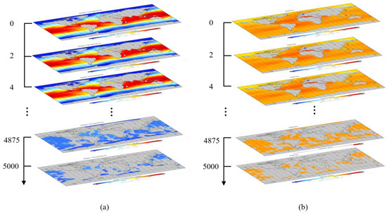
Figure 3.
Original HYCOM data. (a) Temperature data; (b) salinity data.
3.2. Data Processing
For the downloaded original HYCOM data, first, the data for the target area are extracted based on the longitude and latitude of the selected target instruments. After extraction, the data at each time point include nine sets of temperature and salinity profiles each, and the extracted temperature and salinity data are shown in Figure 4.
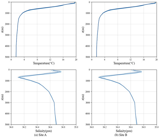
Figure 4.
Temperature–salinity profiles after preprocessing at 00:00 on 1 January 2005. (a) Temperature–salinity profile at Site A; (b) temperature–salinity profile at Site B.
To reconstruct the SSP using the temperature and salinity data extracted above, it is first essential to select an appropriate empirical formula for seawater sound speed. Since the 20th century, researchers in marine science have proposed various empirical formulas to calculate seawater sound speed for SSP reconstruction [41]. Based on the extracted temperature and salinity data, this paper chooses the Mackenzie empirical formula, considering the applicable range of different formulas for sound speed. The Mackenzie empirical formula is suitable for most sea regions worldwide and can be expressed as follows:
In the formula, c is the sound speed measured in m/s, T is the temperature in degrees Celsius, S is the salinity in psu, and z is the seawater depth in meters. The maximum depth for applying the Mackenzie empirical formula for sound speed is 8000 m.
Based on the extracted temperature and salinity data, the SSP of the target research area is calculated using the Mackenzie empirical formula for sound speed. An analysis of the reconstructed SSP shows that its maximum depth is 5000 m. However, the deployment depths of the target PIES instruments all exceed 5000 m. For research convenience, this paper interpolates the SSP of the target research area within the ranges of [0, 5853] and [0, 5961] at 1 m intervals. The interpolated SSP in the research area is shown in Figure 5.
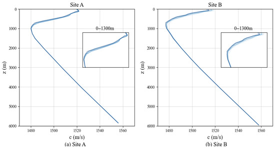
Figure 5.
Interpolated Mackenzie SSPs at Site A and Site B at 00:00:00 on January 1, 2005. (a) SSP at Site A; (b) SSP at Site B.
3.3. Dimensionality Reduction of Seawater Sound Speed Profile
After the data processing described in Section 3.2, we obtain 2920 SSPs in the target study area. To reduce the number of parameters to be inverted, this paper uses the EOF method to decompose the interpolated SSPs separately. EOF models the relationship of SSP variation with depth and ultimately summarizes the main variations in the original data with a small number of modes.
The main process of decomposing SSP using EOF is outlined in Figure 6. It starts with calculating the average SSP, then finding the difference. Next, the covariance matrix R is obtained through decomposition, followed by eigenvalue decomposition of R. The eigenvalues are sorted in descending order, and the relevant eigenvectors are chosen as basis functions based on their contribution rate. The eigenvalues linked with these basis functions become the parameters to be inverted.
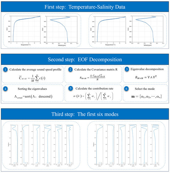
Figure 6.
Flowchart of EOF decomposition.
Figure 7 presents the proportion analysis of the first six modes following EOF decomposition in the SSP. The analysis indicates that the first six eigenvalues account for 98.83% and 99.39% of the total, respectively. When performing SSP inversion, it is important to consider factors such as computational resources; therefore, selecting the first three eigen coefficients as parameters is recommended [42,43].
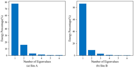
Figure 7.
Analysis diagram of energy proportion of the first twelve modes at Site A and Site B. (a) Energy proportion analysis diagram of Site A; (b) energy proportion analysis diagram of Site B.
Figure 8 displays the first six basis functions obtained from EOF decomposition. Analysis of the figure reveals that, for monitoring Sites A and B, perturbations in the SSP are primarily concentrated within the 0–2000 m range, with abrupt changes in the surface layer. Variations are minimal below 2000 m; at a certain depth, governed by the stable temperature–salinity structure, parameter fluctuations tend to stabilize, and the sound speed shows clear vertical stratification.
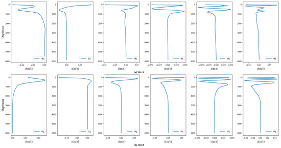
Figure 8.
Analysis diagram of the first six modes at Site A and Site B. (a) First six modes of Site A; (b) first six modes of Site B.
3.4. Inversion Experiment of the Measured Seawater Sound Speed Profile
This paper performs inversion experiments of measured SSPs for Site A and Site B, as listed in Table 1. The experimental process follows Figure 9. All tests were carried out on a ThinkBook 14 G6+ IMH laptop. Its hardware configuration mainly includes an Intel Core Ultra 9 185H processor (with a base clock speed of 2.30 GHz), 32.0 GB of RAM (31.6 GB available during the experiments), multiple GPUs with a total dedicated video memory of 8 GB, 954 GB of internal storage, and Windows 11 Home Chinese Edition (Version 24H2, OS Build 26100.4652).
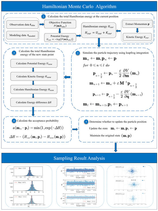
Figure 9.
Flowchart of the experiment for SSP inversion based on the HMC algorithm.
The acoustic propagation time data, measured by the two PIES instruments at different times on 5 April, are used for the experiments. The selected data and their corresponding times are shown in Table 2. For the inversion, the HMC algorithm uses 80 steps for Site A and 120 steps for Site B, with step sizes of [1 × 10⁻², 1 × 10⁻⁴, 1 × 10⁻³] for both. The total number of samples for the two sites is 50,000.
Table 2.
Acoustic propagation experimental data.
Specifically, Figure 10 and Figure 11 display the sampling histograms of the HMC algorithm at different times for Sites A and B, respectively, while Figure 12 and Figure 13 illustrate the sampling trajectories. It can be seen from the sampling histograms that the posterior distributions of the target parameters are all unimodal, smooth, and symmetric, indicating that the HMC algorithm adequately samples the posterior distributions and can effectively characterize the probability distribution characteristics of the model parameters. From the sampling trajectory diagrams of the two sites, it is clear that the sampling results converge to a stable state, confirming that the HMC algorithm can efficiently and sufficiently explore the posterior distributions of the target parameters.
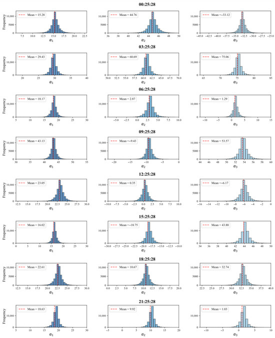
Figure 10.
Sampling histogram of Site A.
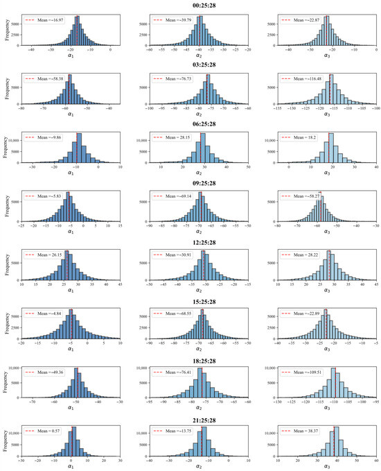
Figure 11.
Sampling histogram of Site B.
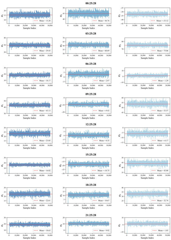
Figure 12.
Sampling trajectory plot of Site A.
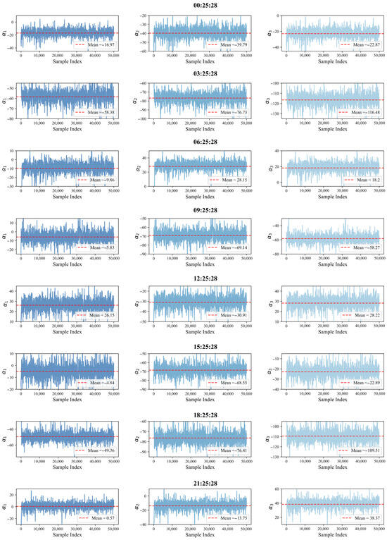
Figure 13.
Sampling trajectory plot of Site B.
Analysis of the histograms shows that, at the same time, the distributions of some parameters vary in width. A wider distribution signifies greater uncertainty in the parameter, while a narrower one indicates lower uncertainty. For the same parameter, the histograms at Site B are consistently wider than those at Site A. For example, at 6:25:28, the distribution of parameter at Site B is narrower, reflecting higher uncertainty in its parameter estimates.
Figure 14 and Figure 15 show error bar plots for Sites A and B. Compared to the error bar plot for Site B, the parameter points at some times in the error bar plot for Site A are more tightly clustered, and the error range (length of the blue lines) is smaller, indicating lower parameter uncertainty and more stable estimation. This is supported by the sharp peak and narrow distribution features of the corresponding histograms.
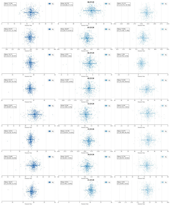
Figure 14.
Error bar plot of Site A.
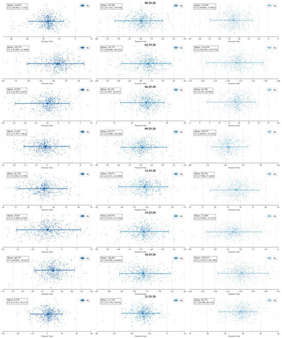
Figure 15.
Error bar plot of Site B.
For the same parameter at different times within the same site, the length of error bars and the distribution of points vary significantly. For example, at Site A, the error bar of at 00:25:28 is longer than that at 03:25:28; this phenomenon may be caused by changes in environmental factors.
At the same time, the error bars of parameter at Site A are all smaller than those of , indicating that is less affected by the model and environment and its estimation is more reliable, while is more sensitive to perturbations. This may be because corresponds to the deep-layer parameter of the SSP, which is significantly influenced by ocean dynamic processes.
Figure 16 presents the comparison diagram of inverted SSPs at different times for the two sites. Combined with the error bar plots and histograms, it can be observed that the fitting degree between the interpolated SSP (solid line) and the HMC-inverted SSP (dashed line) varies dynamically with sites and times. Due to the more stable marine environment and higher data quality at Site B, the fitting degree of its inverted curves is consistently higher than that at Site A.
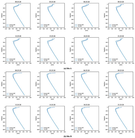
Figure 16.
SSP inversion results of Sites A and B. (a) SSP inversion result of Site A; (b) SSP inversion result of Site B.
Table 3 shows the mean values, acceptance rates, and RMSE of the first three Empirical Orthogonal Function values inverted at various times for the two sites using the same number of samples. The acceptance rate at Site A is lower than at Site B, indicating that the HMC algorithm has greater exploration capability at Site B and can generate samples more efficiently. In terms of Root Mean Square Errors (RMSEs), the average RMSE at Site A is about 3.82 m/s, while at Site B, it is approximately 3.53 m/s, implying that the accuracy of the inverted SSP at Site B is better than at Site A.
Table 3.
Inversion results of the two sites.
4. Discussion and Conclusions
4.1. Discussion
Although the experimental results in this paper have demonstrated the feasibility of inverting the seawater SSP using the HMC algorithm, due to limitations in the experimental design and the inherent defects of the HMC algorithm, there are still some shortcomings in the application of this method to practical problems.
In this study, we used the Mackenzie empirical sound speed formula. Compared to more accurate empirical formulas like the UNESCO empirical formula, the Mackenzie formula primarily considers factors such as temperature, salinity, and depth, while ignoring subtle influences like pressure at different latitudes and longitudes on sound speed. In situations with deep-sea high pressure, high temperature, and high salinity, using depth as an approximation for pressure in the Mackenzie formula can lead to deviations between the inverted and actual sound speeds. Additionally, the UNESCO empirical formula explicitly includes the interactive effects of temperature, salinity, and pressure, but the Mackenzie formula does not adequately account for the interactions among these variables. This limitation may cause the inverted SSP in regions with significant temperature and salinity changes to fail in accurately reflecting the true sound speed layer structure.
Step size and the number of steps are crucial hyperparameters of the HMC algorithm. During SSP inversion using HMC, we observed that setting these parameters greatly impacts the results. When the number of steps remains fixed, a very small step size can cause the sampler to get stuck in local optima, while an excessively large step size can lead to many samples being rejected, wasting computational resources. Fixing the step size and varying the number of steps show that too few steps do not explore the sample space adequately, whereas too many steps waste unnecessary resources. The need for manual tuning of the step size and number of steps makes the HMC algorithm less practical for real-world problems. Luckily, its improved version, the No-U-Turn Sampler (NUTS), automatically adjusts these parameters, greatly improving the algorithm’s adaptability. Future research will focus on using NUTS to enhance the accuracy and efficiency of SSP inversion.
The HMC algorithm assumes that the parameter space is a Euclidean space, and the kinetic energy of its auxiliary variables often has a fixed mass matrix. However, in the SSP inversion problem, the posterior distribution of the target parameters shows extremely large curvatures in different directions. In such cases, HMC struggles to adapt to the local curvatures of the posterior distribution, leading to low sampling efficiency and a small number of effective sampling points.
Unlike the HMC algorithm, the Riemannian Manifold Hamiltonian Monte Carlo (RMHMC) algorithm can adaptively match the geometric features of the parameter space by using a mass matrix that depends on the current parameters. Therefore, it can explore the distribution of the target parameters more efficiently. In future research, we will further examine the performance of RMHMC in SSP inversion.
4.2. Conclusions
This paper introduces a method for inverting seawater SSP based on the HMC algorithm, which integrates EOF dimensionality reduction technology to enable real-time reconstruction of seawater SSP inversion. Experimental results show that the average RMSE of SSP inversion using the HMC algorithm can reach 3.82 m/s and 3.53 m/s, respectively, confirming the feasibility of using the HMC algorithm for SSP inversion. For the EOF coefficients of SSP, the HMC algorithm can analyze uncertainty from their posterior distribution, calculate confidence intervals, and quantify the credibility of the inversion results, helping researchers make objective and comprehensive decisions within a certain range.
Author Contributions
Conceptualization, S.M. and J.Z.; methodology, J.Z. and S.M.; software, J.Z.; validation, J.Z.; formal analysis, J.Z.; investigation, S.M. and J.Z.; resources, S.M., J.Z. and Q.L.; data curation, J.Z.; writing—original draft preparation, J.Z.; writing—review and editing, J.Z. and S.M.; visualization, J.Z.; supervision, J.Z. and S.M.; project administration, S.M. and Q.L. All authors have read and agreed to the published version of the manuscript.
Funding
This research was funded by National Natural Science Foundation of China (Grant No.42176197).
Data Availability Statement
The authors thank the Hybrid Coordinate Ocean Model (HYCOM) for providing temperature and salinity profile data (https://www.hycom.org/, accessed on 18 July 2025), and the Kuroshio Extension System Study (KESS) project for providing acoustic propagation time data (https://www.po.gso.uri.edu/dynamics/KESS/CPIES_data.html, accessed on 19 July 2025).
Acknowledgments
The authors thank the reviewers and editors for their constructive comments on this work.
Conflicts of Interest
The authors declare no conflicts of interest.
Appendix A
The pseudocode of the HMC algorithm used in SSP is shown in Algorithm A1 (Pseu-docode for HMC).
| Algorithm A1 Hamiltonian Monte Carlo |
| Output: Target parameter samples Q do |
do 11: if (l < L) then 13: end if 14: end for )) then 21: else |
| 23: end if 25: End for |
References
- Klausner, N.H.; Azimi-Sadjadi, M.R. Performance Prediction and Estimation for Underwater Target Detection Using Multichannel Sonar. IEEE J. Ocean. Eng. 2020, 45, 534–546. [Google Scholar] [CrossRef]
- Ghafoor, H.; Noh, Y. An Overview of Next-Generation Underwater Target Detection and Tracking: An Integrated Underwater Architecture. IEEE Access 2019, 7, 98841–98853. [Google Scholar] [CrossRef]
- Luo, J.; Han, Y.; Fan, L. Underwater Acoustic Target Tracking: A Review. Sensors 2018, 18, 112. [Google Scholar] [CrossRef]
- Cato, D.; McCauley, R.; Rogers, T.; Noad, M. Passive Acoustics for Monitoring Marine Animals—Progress and Challenges. In Proceedings of the Australian Acoustical Society Conference (ACOUSTICS 2006), Christchurch, New Zealand, 20–22 November 2006. [Google Scholar]
- Cominelli, S.; Bellin, N.; Brown, C.D.; Rossi, V.; Lawson, J. Acoustic Features as a Tool to Visualize and Explore Marine Soundscapes: Applications Illustrated Using Marine Mammal Passive Acoustic Monitoring Datasets. Ecol. Evol. 2024, 14, e10951. [Google Scholar] [CrossRef]
- Guan, S.; Brookens, T.; Vignola, J. Use of Underwater Acoustics in Marine Conservation and Policy: Previous Advances, Current Status, and Future Needs. J. Mar. Sci. Eng. 2021, 9, 173. [Google Scholar] [CrossRef]
- Liu, Y.; Li, S.; Zou, Z.; Sun, Y. Techniques and Methods for Seafloor Topography Mapping: Past, Present, and Future. Intell. Mar. Technol. Syst. 2025, 3, 8. [Google Scholar] [CrossRef]
- Yu, X.; Zhai, J.; Zou, B.; Shao, Q.; Hou, G. A Novel Acoustic Sediment Classification Method Based on the K-Mdoids Algorithm Using Multibeam Echosounder Backscatter Intensity. J. Mar. Sci. Eng. 2021, 9, 508. [Google Scholar] [CrossRef]
- Edelmann, G.F.; Lingevitch, J.F.; Gemba, K.L. Through the Sensor Estimation of Sound Speed Profiles. J. Acoust. Soc. Am. 2024, 155, 1534–1545. [Google Scholar] [CrossRef]
- Li, J.; Shi, Y.; Yang, Y.; Chen, C. Comprehensive Study of Inversion Methods for Sound Speed Profiles in the South China Sea. J. Ocean Univ. China 2022, 21, 1487–1494. [Google Scholar] [CrossRef]
- Cho, B.; Makris, N.C. Predicting the Effects of Random Ocean Dynamic Processes on Underwater Acoustic Sensing and Communication. Sci. Rep. 2020, 10, 4525. [Google Scholar] [CrossRef]
- Munk, W.; Wunsch, C. Ocean Acoustic Tomography: A Scheme for Large Scale Monitoring. Deep Sea Res. Part A Oceanogr. Res. Pap. 1979, 26, 123–161. [Google Scholar] [CrossRef]
- Huang, W.; Zhou, J.; Gao, F.; Lu, J.; Li, S.; Wu, P.; Wang, J.; Zhang, H.; Xu, T. Underwater Sound Speed Profile Construction: A Review. J. Mar. Sci. Eng. 2024, 12, 2356. [Google Scholar] [CrossRef]
- Bianco, M.J.; Gerstoft, P.; Traer, J.; Ozanich, E.; Roch, M.A.; Gannot, S.; Deledalle, C.-A. Machine Learning in Acoustics: Theory and Applications. J. Acoust. Soc. Am. 2019, 146, 3590–3628. [Google Scholar] [CrossRef] [PubMed]
- Carriere, O.; Hermand, J.-P.; Candy, J.V. Inversion for Time-Evolving Sound-Speed Field in a Shallow Ocean by Ensemble Kalman Filtering. IEEE J. Ocean. Eng. 2009, 34, 586–602. [Google Scholar] [CrossRef]
- Tolstoy, A.; Diachok, O.; Frazer, L.N. Acoustic Tomography via Matched Field Processing. J. Acoust. Soc. Am. 1991, 89, 1119–1127. [Google Scholar] [CrossRef]
- Skarsoulis, E.K.; Athanassoulis, G.A.; Send, U. Ocean Acoustic Tomography Based on Peak Arrivals. J. Acoust. Soc. Am. 1996, 100, 797–813. [Google Scholar] [CrossRef]
- Qu, K.; Piao, S.-C.; Zhu, F.-Q. A noval method of constructing shallow water sound speed profile based on dynamic characteristic of internal tides. Acta Phys. Sin. 2019, 68, 124302. [Google Scholar] [CrossRef]
- Zhang, C.; Zhu, Z.-N.; Xiao, C.; Zhu, X.-H.; Liu, Z.-J. Acoustic Tomographic Inversion of 3D Temperature Fields with Mesoscale Anomaly in the South China Sea. Front. Mar. Sci. 2024, 11, 1350337. [Google Scholar] [CrossRef]
- Huang, W.; Zhou, J.; Gao, F.; Wang, J.; Xu, T. Experimental Results of Underwater Sound Speed Profile Inversion by Few-Shot Multi-Task Learning. Remote Sens. 2023, 16, 167. [Google Scholar] [CrossRef]
- Radhakrishnan, S.; Anilkumar, K. Inversion for Water Column Sound Speed Profile from Acoustic Travel Times Using Empirical Orthogonal Functions. J. Acoust. Soc. Am. 2024, 156, 4061–4072. [Google Scholar] [CrossRef]
- Wu, P.; Zhang, H.; Shi, Y.; Lu, J.; Li, S.; Huang, W.; Tang, N.; Wang, S. Real-Time Estimation of Underwater Sound Speed Profiles with a Data Fusion Convolutional Neural Network Model. Appl. Ocean Res. 2024, 150, 104088. [Google Scholar] [CrossRef]
- Earl, D.J.; Deem, M.W. Parallel Tempering: Theory, Applications, and New Perspectives. Phys. Chem. Chem. Phys. 2005, 7, 3910. [Google Scholar] [CrossRef]
- Gerstoft, P.; Mecklenbräuker, C.F. Ocean Acoustic Inversion with Estimation of a Posteriori Probability Distributions. J. Acoust. Soc. Am. 1998, 104, 808–819. [Google Scholar] [CrossRef]
- Fichtner, A.; Zunino, A.; Gebraad, L. Hamiltonian Monte Carlo Solution of Tomographic Inverse Problems. Geophys. J. Int. 2019, 216, 1344–1363. [Google Scholar] [CrossRef]
- Lytaev, M. Automatically Differentiable Higher-Order Parabolic Equation for Real-Time Underwater Sound Speed Profile Sensing. J. Mar. Sci. Eng. 2024, 12, 1925. [Google Scholar] [CrossRef]
- Xu, G.; Qu, K.; Li, Z.; Zhang, Z.; Xu, P.; Gao, D.; Dai, X. Enhanced Inversion of Sound Speed Profile Based on a Physics-Inspired Self-Organizing Map. Remote Sens. 2025, 17, 132. [Google Scholar] [CrossRef]
- Liu, Y.; Chen, Y.; Chen, W.; Meng, Z. Inversion of Sound Speed Profile in the Luzon Strait by Combining Single Empirical Orthogonal Function and Generalized Regression Neural Network. IEEE Geosci. Remote Sens. Lett. 2024, 21, 1502405. [Google Scholar] [CrossRef]
- Dosso, S.E.; Nielsen, P.L. Quantifying Uncertainty in Geoacoustic Inversion. II. Application to Broadband, Shallow-Water Data. J. Acoust. Soc. Am. 2002, 111, 143–159. [Google Scholar] [CrossRef]
- Dosso, S.E. Quantifying Uncertainty in Geoacoustic Inversion. I. A Fast Gibbs Sampler Approach. J. Acoust. Soc. Am. 2002, 111, 129–142. [Google Scholar] [CrossRef]
- De Figueiredo, L.P.; Grana, D.; Roisenberg, M.; Rodrigues, B.B. Multimodal Markov Chain Monte Carlo Method for Nonlinear Petrophysical Seismic Inversion. Geophysics 2019, 84, M1–M13. [Google Scholar] [CrossRef]
- Dettmer, J.; Dosso, S.E.; Holland, C.W. Uncertainty Estimation in Seismo-Acoustic Reflection Travel Time Inversion. J. Acoust. Soc. Am. 2007, 122, 161–176. [Google Scholar] [CrossRef]
- Wu, P.; Sun, J. A Method for Velocity Inversion of Deep-Sea Water Body Using Wave Equation Traveltime. IEEE Trans. Geosci. Remote Sens. 2025, 63, 4200208. [Google Scholar] [CrossRef]
- De Figueiredo, L.P.; Grana, D.; Roisenberg, M.; Rodrigues, B.B. Gaussian Mixture Markov Chain Monte Carlo Method for Linear Seismic Inversion. Geophysics 2019, 84, R463–R476. [Google Scholar] [CrossRef]
- Betancourt, M. A Conceptual Introduction to Hamiltonian Monte Carlo. arXiv 2018, arXiv:1701.02434. [Google Scholar] [CrossRef]
- Neal, R.M. MCMC Using Hamiltonian Dynamics. arXiv 2012, arXiv:1206.1901. [Google Scholar] [CrossRef]
- Dosso, S.E.; Holland, C.W.; Sambridge, M. Parallel Tempering for Strongly Nonlinear Geoacoustic Inversion. J. Acoust. Soc. Am. 2012, 132, 3030–3040. [Google Scholar] [CrossRef]
- Davis, R.E. Predictability of Sea Surface Temperature and Sea Level Pressure Anomalies over the North Pacific Ocean. J. Phys. Oceanogr. 1976, 6, 249–266. [Google Scholar] [CrossRef]
- Metropolis, N.; Rosenbluth, A.W.; Rosenbluth, M.N. Equation of State Calculations by Fast Computing Machines. J. Chem. Phys. 1953, 21, 1087–1092. [Google Scholar] [CrossRef]
- Zunino, A.; Ghirotto, A.; Armadillo, E.; Fichtner, A. Hamiltonian Monte Carlo Probabilistic Joint Inversion of 2D (2.75D) Gravity and Magnetic Data. Geophys. Res. Lett. 2022, 49, e2022GL099789. [Google Scholar] [CrossRef]
- Mackenzie, K.V. Nine-Term Equation for Sound Speed in the Oceans. J. Acoust. Soc. Am. 1981, 70, 807–812. [Google Scholar] [CrossRef]
- Golubović, D.; Vukmirović, N.; Erić, M.; Simić-Pejović, M. Method for Noise Subspace Determination in HFSWR’s High-Resolution Range-Doppler Map Estimation. In Proceedings of the 2023 10th International Conference on Electrical, Electronic and Computing Engineering (IcETRAN), East Sarajevo, Bosnia and Herzegovina, 5–8 June 2023; IEEE: Piscataway, NJ, USA; pp. 1–6. [Google Scholar]
- Golubović, D.; Marjanović, D. An Experimentally-Based Method for Detection Threshold Determination in HFSWR’s High-Resolution Range-Doppler Map Target Detection. In Proceedings of the 2025 24th International Symposium INFOTEH-JAHORINA (INFOTEH), East Sarajevo, Bosnia and Herzegovina, 19–21 March 2025; IEEE: Piscataway, NJ, USA; pp. 1–6. [Google Scholar]
Disclaimer/Publisher’s Note: The statements, opinions and data contained in all publications are solely those of the individual author(s) and contributor(s) and not of MDPI and/or the editor(s). MDPI and/or the editor(s) disclaim responsibility for any injury to people or property resulting from any ideas, methods, instructions or products referred to in the content. |
© 2025 by the authors. Licensee MDPI, Basel, Switzerland. This article is an open access article distributed under the terms and conditions of the Creative Commons Attribution (CC BY) license (https://creativecommons.org/licenses/by/4.0/).