Analysis of the Impact of Curvature Correction Factor f_c on the Flow Past a Two-Dimensional Bluff Body

Abstract

This paper presents an improved k-ω SST turbulence model to enhance the simulation accuracy of Bluff Body Bypassing Problems (BBBPs) within the Reynolds-Averaged Navier–Stokes (RANS) framework. Although RANS methods are computationally efficient, they are limited in resolving instantaneous turbulent fluctuations, which often results in significant errors when predicting turbulent kinetic energy variations in complex flows. To address this, a curvature correction factor (f_c) is introduced into the production term (P_k) of the turbulent kinetic energy equation. This factor is derived from the local fluid rotational rate, enabling the model to better account for streamline curvature effects and unsteady vortex dynamics. The modified model, along with the baseline k-ω SST formulation, is applied to two-dimensional (2D) square column flow cases. Numerical results show that the corrected model significantly improves predictive accuracy, reducing the error in the time-averaged drag coefficient (C_D) from 24% to 8.3%, thereby demonstrating its effectiveness in capturing key flow characteristics around bluff bodies.

1. Introduction

Flow past a bluff body is a classical problem in fluid dynamics that is frequently encountered in engineering applications, such as wind flow around buildings [1], river flow past bridge piers [2,3,4], cooling tower ventilation [5], the descent of ships and aircraft in water, and biological phenomena such as whale falls. When the fluid bypasses the surface of a bluff body, vortices are generated and shed in the wake region, producing periodic pressure fluctuations. These fluctuations can induce structural vibrations, which become particularly dangerous when the vibration frequency approaches the natural frequency of the structure, potentially leading to resonance, fatigue, and even catastrophic structural failure. A notable historical example is the collapse of the Tacoma Narrows Bridge in the United States, which was attributed to torsional oscillations triggered by wind-induced vortex shedding. This highlights the importance of understanding the mechanisms and influencing factors of flow past bluff bodies, especially the formation of vortices and strategies to suppress or control induced vibrations.

In recent decades, both experimental and computational studies on bluff body flows have been extensively conducted. Sen [6] and Zhu and Holmedal [7] examined the mechanical characteristics of elliptical cylinders, while Chaitanya [8] and Miran and Sohn [9] focused on the flow behavior around two-dimensional (2D) square columns. Yadav et al. [10], Liu et al. [11], and Masoudi et al. [12] investigated flow fields around prismatic geometries. Two primary research approaches are widely adopted: experimental methods and computational fluid dynamics (CFD).

For experimental studies, Larose and D’Auteuil [13], Dutta et al. [14], van Hinsberg et al. [15], and others have explored the key parameters affecting square column flow, including the Reynolds number, incidence angle, and corner radius. Lyn [16], Durao [17], and Lee [18] employed laser Doppler anemometry to measure drag and lift coefficients at Reynolds numbers ranging from 2.2 × 104 to 1.4 × 104 and 1.76 × 105. These results often serve as benchmarks for CFD validation. The experimental method is highly accurate, but with a long research period and substantial infrastructure requirements. With the rapid development of computer hardware technology, the CFD method based on viscous hydrodynamics is widely used in the study of the flow past airfoils and bluff bodies because of its low cost and high computational efficiency and reliability.

Common CFD approaches include Direct Numerical Simulation (DNS) [19], Large-Eddy Simulation (LES) [20], and Reynolds-Averaged Navier–Stokes (RANS) [21] methods. DNS resolves all scales of turbulent motion and provides the highest accuracy but is limited by its extreme computational cost, making it impractical for most engineering applications. LES captures large-scale turbulent structures and models the sub-grid scales, providing a balance between accuracy and computational feasibility. For instance, Kim et al. [22] used LES to simulate vortex shedding behind square columns, achieving results in good agreement with experimental data. Wu [23] applied LES under sliding boundary conditions to simulate square column bypassing, while Ricardo et al. [24] compared RANS, LES, and hybrid RANS/LES simulations against experimental results to assess their relative accuracy and computational performance. In recent studies, machine learning techniques have also been combined with LES [25,26,27] to improve prediction accuracy and computational efficiency. However, LES still requires a high mesh resolution and significant computational resources, particularly for transient simulations.

To improve the computational efficiency, a variety of simplification methods have been developed in the field of fluid dynamics, among which the RANS equation model is a tested method suitable for engineering solutions. For the flow past a bluff body, a fluid mass that passes around the surface of a bluff body produces a vortex due to strong rotation, and the turbulent kinetic energy varies periodically. The RANS method can obtain the mean flow field, but it cannot obtain the instantaneous turbulent fluctuations, which makes it difficult to capture the variation rule of turbulent kinetic energy in the flow field; hence, the computational accuracy is lower than that of the DNS and LES. In this paper, to accurately predict the variation rule of turbulent kinetic energy in the bluff body problems and to increase the simulation accuracy of the RANS method for solving the flow past a bluff body, we propose certain modifications to the original k-ω SST turbulence model, i.e., using a closed set of equations for the k-ω SST turbulence model and introducing a streamline curvature correction factor (f_c). This modification corrects the turbulent kinetic energy resultant term (P_k) in the transport equation of the k-ω SST turbulence model based on the rotational rate of local fluid mass, therefore making it feasible to accurately capture instantaneous flow field characteristics. The effectiveness of the proposed correction is investigated in three stages. First, the influence of f_c on airflow around airfoils is evaluated using published experimental data for two-dimensional airfoils. Second, the impact of f_c on bluff body flow is analyzed using experimental data for the flow past a two-dimensional square cylinder. Finally, a parametric study is conducted to examine the effect of f_c on the flow around a 2D square cylinder under various Reynolds numbers and angles of attack.

Compared with the experimental data in the literature, the k-ω SST turbulence model has a high simulation accuracy in solving 2D airfoil bypassing flow problems in which the rotational motion of the fluid plasmas is not intense, and the accuracy is improved after correction by f_c, but the magnitude is limited; the curvature correction factor plays a significant role in solving 2D bluff bypassing flow problems in which vortices vary significantly. However, in the 2D blunt body bypassing problem, where the rotational motion of the fluid plasmas is violent, f_c has a significant effect on the improvement in numerical simulation accuracy, and the prediction error of the time-averaged drag coefficient (C_D) of the 2D square column’s flow reduces from 24% to 8.3% because the k-ω SST turbulence model corrected using f_c can more accurately capture the rotational motion of the fluid mass, the simulated velocity and pressure fields are more realistic, and the time-averaged pressure coefficient (C_P) at the back of the bluff body is closer to the experimental value.

The innovation of this paper lies in its introduction of a correction term, μ_t f_cS², to the P_k equation for improving the k-ω SST turbulence model, which effectively improves the accuracy of the RANS method in solving the flow past a 2D bluff body.

In this paper, Section 2 introduces the turbulence model correction method and mesh parameters; Section 3 analyzes the effect of the f_c on the flow past a 2D airfoil; and Section 4 and Section 5 analyze the effect of f_c on the flow past a 2D bluff body. The simulations in this study were carried out using STAR-CCM+.

2. CFD Simulation Method

2.1. Numerical Method

RANS equations involve averaging the unsteady flow-governing equations over time, capturing only large-scale time-averaged flow behavior. They have been widely applied in CFD analyses in hydrodynamics and aerodynamics. The general form of the RANS equations is expressed as follows:

$${\displaystyle \frac{\partial \left(\rho U\right)}{\partial t}}+\nabla \cdot \left(\rho U\otimes U\right)=\rho f+\nabla \cdot \left\{-p\delta +\mu \left\{\nabla U+{\displaystyle \frac{1}{3}}{\left(\nabla U\right)}^T\right\}\right\}-\nabla \cdot \left(\rho \overline{U}\otimes \overline{U}\right)$$

(1)

Compared with the Navier–Stokes (N-S) equations, which describe the instantaneous flow field, RANS equations are almost identical except for the presence of additional Reynolds stress terms. These terms account for the non-zero fluctuating velocities during the time-averaging process. The challenge in solving flow field problems using RANS equations lies in the fact that the number of unknowns exceeds the number of equations, resulting in an unclosed system. To address this closure problem, turbulence models are introduced to relate the Reynolds stresses to the mean flow quantities and thereby close the equations.

2.2. Turbulence Model

Turbulence models can be classified into several categories, including zero-equation, one-equation, and two-equation models. Among them, two-equation models, such as the k-ε and k-ω models, are the most widely used in engineering applications.

The k-ε model is a semi-empirical formula approach that, in many cases, yields satisfactory results in flow field analyses. However, it can encounter convergence difficulties when applied to rotational flows or flows involving significant boundary layer separation.

The k-ω model solves the transport equations for turbulent kinetic energy (k) and turbulence frequency (ω) to determine turbulent eddy viscosity. The k-ω model has been algorithmically optimized to address issues of boundary layer separation caused by adverse pressure gradients, making it particularly effective in flow problems dominated by turbulent boundary layers. In the k-ω model, k is as follows:

$${\displaystyle \frac{\partial \rho k}{\partial t}}+\nabla \cdot \left(\rho \overline{\mathit{U}}k\right)=\nabla \cdot \left\{\left(\mu +{\sigma }_k{\mu }_t\right)\nabla k\right\}+P_k-{\beta }^{\prime }\rho k\omega$$

(2)

ω is as follows:

$${\displaystyle \frac{\partial \rho \omega }{\partial t}}+\nabla \cdot \left(\rho \overline{\mathit{U}}\omega \right)=\nabla \cdot \left\{\left(\mu +{\sigma }_{\omega }{\mu }_t\right)\nabla \omega \right\}+P_{\omega }-\beta \rho {\omega }^2$$

(3)

where

• $\overline{\mathit{U}}$ is the average velocity;
• $\mu$ is the dynamic viscosity;
• ${\mu }_t$ is the eddy viscosity, ${\mu }_t=\rho {\displaystyle \frac{k}{\omega }}$;
• $P_k$ is the result term of the turbulent kinetic energy, $P_k=-{\displaystyle \frac{2}{3}}\rho k\nabla \cdot \overline{\mathit{U}}-{\displaystyle \frac{2}{3}}{\mu }_t{\left(\nabla \cdot \overline{\mathit{U}}\right)}^2$;
• $P_{\omega }$ is the turbulence frequency result term, $P_{\omega }=\rho \gamma \left[\left(S^2-{\displaystyle \frac{2}{3}}{\left(\nabla \cdot \overline{\mathit{U}}\right)}^2\right)-{\displaystyle \frac{2}{3}}\omega \nabla \cdot \overline{\mathit{U}}\right]$;

$S$ is the modulus of the average strain rate tensor S, $S=\left|\mathit{S}\right|=\sqrt{2\mathit{S}:{\mathit{S}}^T}=\sqrt{2\mathit{S}:\mathit{S}}$;

$$\mathit{S}={\displaystyle \frac{1}{2}}\left(\nabla \overline{\mathit{U}}+\nabla {\overline{\mathit{U}}}^T\right).$$

The constant values in the k-ω model are shown in

Table 1. Constant values of the k-ω model.

${\sigma }_k$	${\sigma }_{\omega }$	$\beta$	${\beta }^{\prime }$
0.5	0.5	0.072	0.09

.

Menter [28] demonstrated that the transport equation for the turbulence dissipation rate (ε) in the k-ε model can be transformed into a transport equation for ω through a variable substitution. This transformed equation is similar to that in the k-ω model but includes an additional non-conservative cross-diffusion term, which incorporates the dot product. By incorporating this term into the transport equation of the k-ω model, the high sensitivity issue of the k-ε model in calculating free streams within the boundary layer is addressed. Furthermore, Menter corrected the linear constitutive equations. By deriving constitutive relations from Reynolds stress models, the k-ω model achieves a higher simulation accuracy in anisotropic turbulence. This modified turbulence model is named the k-ω SST (Shear Stress Transport) model. The model coefficients are specified in Equations (4)–(8):

$${\sigma }_k=F_1{\sigma }_{k_1}+\left(1-F_1\right){\sigma }_{k_2}$$

(4)

$${\sigma }_{\omega }=F_1{\sigma }_{{\omega }_1}+\left(1-F_1\right){\sigma }_{{\omega }_2}$$

(5)

$$\beta =F_1{\beta }_1+\left(1-F_1\right){\beta }_2$$

(6)

$${\beta }^{\prime }=F_1{{\beta }^{\prime }}_1+\left(1-F_1\right){\beta }_2^{\prime }$$

(7)

$$F_1=\tanh \left({\left[\min \left(\max \left({\displaystyle \frac{\sqrt{k}}{0.09wd}},{\displaystyle \frac{500v}{d^2\omega }}\right),{\displaystyle \frac{2k}{d^{2}C{D}_{kw}}}\right)\right]}^4\right)$$

(8)

where

• $d$ is the distance between the grid node and the wall surface;
• $\nu$ is the kinematic viscosity;
• $C{D}_{kw}$ is the cross-diffusion coefficient, $C{D}_{kw}=\max \left({\displaystyle \frac{1}{\omega }}\nabla k\cdot \nabla \omega ,{10}^{-20}\right)$.

The required constant values for each coefficient are shown in

Table 2. Constant values of the k-ω SST model.

${\sigma }_{k_1}$	${\sigma }_{k_2}$	${\sigma }_{{\omega }_1}$	${\sigma }_{{\omega }_2}$	${\beta }_1$	${\beta }_2$	${\beta }_1^{\prime }$	${\beta }_2^{\prime }$
0.85	1	0.5	0.856	0.075	0.0828	0.09	0.09

.

Dramatic changes in streamline curvature as flow passes around a bluff body significantly influence the evolution of turbulent quantities. However, due to inherent limitations in their formulation, single-equation and two-equation turbulence models are not intrinsically sensitive to curvature effects. To address this deficiency, we introduce a streamline curvature correction factor (f_c) to enhance the turbulent kinetic energy production term (P_k). The construction of f_c follows a philosophy similar to previously developed rotation and curvature correction models (Arolla & Durbin [29]), where invariants and limiting functions are employed to improve the applicability of turbulence models under rotational and curved flows. This modification is intended not to propose an entirely new functional form but rather to adapt and incorporate such a correction into the k-ω SST framework to better capture the characteristics of bluff body flows. With this correction, the expression for P_k is reformulated as

$$P_k={\mu }_t{f}_c{S}^2-{\displaystyle \frac{2}{3}}\rho k\nabla \cdot \overline{\mathit{U}}-{\displaystyle \frac{2}{3}}{\mu }_t{\left(\nabla \cdot \overline{\mathit{U}}\right)}^2$$

(9)

$$f_c=\min \left(C_{\max },{\displaystyle \frac{1}{C_{r_1}\left(\left|\eta \right|-\eta \right)+\sqrt{1-\min \left(C_{r_2},0.99\right)}}}\right)$$

(10)

where

$$\eta =T^2\left(\mathit{S}:\mathit{S}-\mathit{W}:\mathit{W}\right);$$

$$T=\max \left(T_1,T_2\right);$$

$$T_1={\displaystyle \frac{1}{\beta \ast \omega }};$$

$$T_2={\left(T_1^{1.625}{T}_3\right)}^{{\displaystyle \frac{1}{1.625+1}}};$$

$$T_3=6\sqrt{{\displaystyle \frac{\nu }{\beta \ast k\omega }}}.$$

W is the absolute rotation rate tensor;

• $\mathit{W}={\mathit{W}}^l+{\mathit{W}}^f+\left(C_{ct}-1\right){\mathit{W}}^S$, where ${\mathit{W}}^l$, ${\mathit{W}}^f$, and ${\mathit{W}}^S$ represent the contributions generated by vortices calculated from the local reference coordinate system, rotating reference coordinate system, and streamline curvature, respectively:

$${\mathit{W}}^l={\displaystyle \frac{1}{2}}\left(\nabla \overline{\mathit{U}}-\nabla {\overline{\mathit{U}}}^T\right);$$

$${\mathit{W}}^f=\mathit{E}\cdot {\mathit{\omega }}^f;$$

$${\mathit{W}}^S={\mathit{W}}^f-\mathit{E}\cdot \left({\mathit{A}}^{-1}\cdot \mathit{\omega }\right);$$

$$\mathit{A}=\mathit{I}-{\displaystyle \frac{3{\mathit{S}}^2}{2\mathit{S}:\mathit{S}}};$$

E is the Levi-Civita tensor;

$$\mathit{\omega }=\mathit{E}\cdot {\displaystyle \frac{\mathit{S}\cdot \left(D_t\mathit{S}\right)-\left(D_t\mathit{S}\right)\cdot \mathit{S}}{2\mathit{S}:\mathit{S}}};$$

D_tS is the total derivative tensor of strain rate.

For the model constants $C_{\max }$, $C_{r_1}$, $C_{r_2}$, and $C_{ct}$, the values are taken as 1.25, 0.04645, 0.25, and 2, respectively.

2.3. Wall Treatment Methods

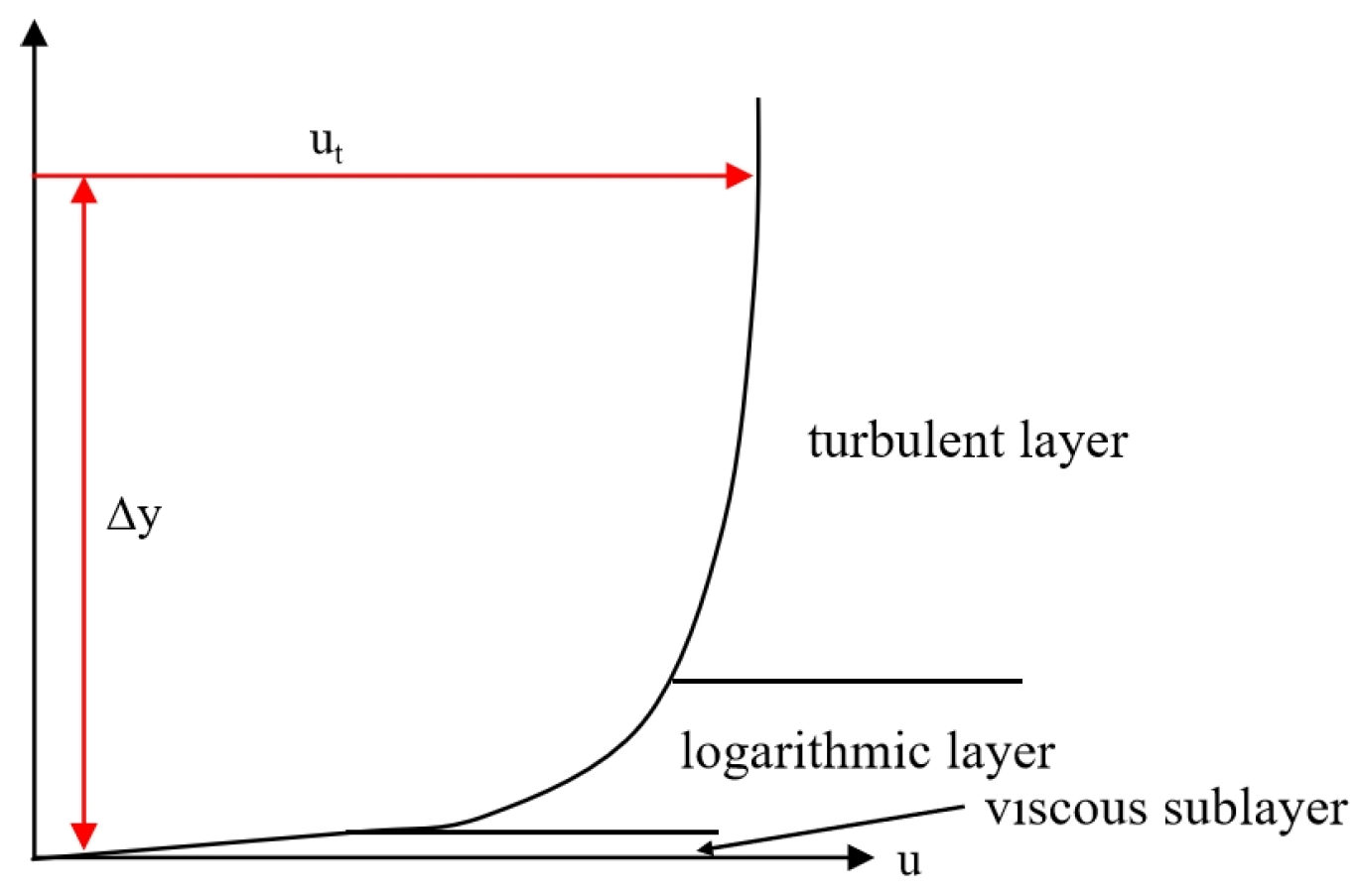
Based on the non-dimensional wall distance (Y+), wall treatment methods in CFD can be categorized into three types: low Y+, high Y+, and all Y+ (also known as hybrid or blended) approaches. The low Y+ method resolves the entire boundary layer, including the thin viscous sublayer, by placing all computational nodes within it, as illustrated in Figure 1. This approach requires a very fine mesh to accurately capture the near-wall gradients and flow characteristics, resulting in high computational costs but also high simulation accuracy. For the near-wall grid cells, Y+ values are typically around 1. The high Y+ employs wall functions to approximate boundary conditions for the governing equations. Wall shear stress, turbulence quantities, and dissipation rates are derived from the equilibrium theory of turbulent boundary layers. This method does not resolve the viscous sublayer, making it suitable for coarser meshes and more efficient in terms of computational resources. In this case, Y+ values near the wall are generally greater than 30. The all Y+ treatment is a hybrid method that combines the advantages of both the low Y+ and high Y+ approaches. It behaves like the low Y+ method when the mesh is sufficiently refined and like the high Y+ method when the mesh is coarse. This approach strikes a balance between simulation accuracy and computational stability. In this study, considering both accuracy and computational efficiency, the all Y+ treatment method is adopted for near-wall modeling.

2.4. Grid Type and Parameters

Meshes in computational fluid dynamics (CFD) are typically categorized into structured and unstructured types according to their geometric arrangement. Structured meshes are composed of orthogonal hexahedral elements, which provide enhanced orthogonality, computational efficiency, and numerical accuracy. However, generating structured meshes becomes challenging for geometries with complex shapes or significant local curvature, where mesh conformity is difficult to maintain. Unstructured meshes, although generally less efficient and slightly less accurate than structured ones, provide much greater flexibility. They are well-suited for domains with intricate geometries due to their adaptability and ability to conform to complex boundaries. Among unstructured mesh types, tetrahedral meshes are the most commonly used. There are two primary methods for generating tetrahedral meshes: the Delaunay method and the Advancing Front method. The Delaunay method generates high-quality tetrahedral elements by incrementally inserting points into the domain. It ensures that the mesh conforms to the triangulated boundary surfaces, making the quality of the initial surface mesh critical for obtaining a high-quality volume mesh. This method is both efficient and resource-conserving and is widely adopted in commercial solvers such as STAR-CCM+ and Pointwise. The Advancing Front method, also known as the front advancing method, builds meshes by advancing from the boundary inward. It produces well-ordered triangular surface meshes and high-quality tetrahedral elements. This approach offers excellent adaptability to complex geometric boundaries but is generally less efficient than the Delaunay method and requires tighter control over various parameters to maintain the mesh’s quality. In this study, a hybrid meshing strategy is adopted: structured meshes are used in the far-field region, while tetrahedral unstructured meshes, generated using the Delaunay method, are applied near the wall. The specific mesh parameters are detailed as follows:

• Total thickness of boundary layer (δ): $\delta \ge 0.064 L {\mathrm{Re}}^{-1/7}$;
• Thickness of the first boundary layer (Δδ): $\Delta \delta \le L{Y}^{+}\sqrt{80} {\mathrm{Re}}^{-13/14}$;
• Number of boundary layers (N): N ≥ 15;
• Face mesh scale (S): S ≤ δ; partial encryption takes 0.5 S and 0.25 S;
• Volume mesh scale (V): V = 20 S; encrypts the 2 S in the near-wall area.

L is the characteristic length, and Re is the Reynolds number based on length.

2.5. Watershed Parameters

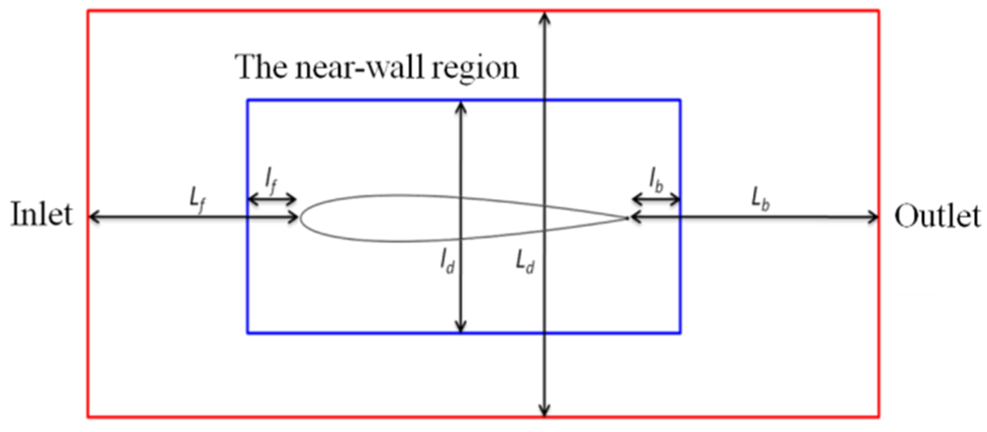
Sohankar [30] and others, through their computational studies on low-Re flow problems, have summarized the parameters for setting up the flow domain, as shown in Figure 2. The settings are as follows:

• The distance from the inlet boundary to the front edge of the simulation model (L_f) should be no less than 15 times the characteristic length (L);
• The distance from the outlet boundary to the rear edge of the simulation model (L_b) should be no less than 25 L;
• The mutual distance between the side boundaries (L_d) should be no less than 20 L;
• The distance from the front end of the near-wall region to the front edge of the simulation model (lf) should be no less than 1.5 L;
• The distance from the rear end of the near-wall region to the rear edge of the simulation model (lb) should be no less than 2.5 L;
• The mutual distance between the side boundaries in the near-wall region (L_d) should be no less than 2 L.

3. Analysis of the Impact of Curvature Correction Factor (${\mathit{f}}_{\mathit{c}}$) on 2D Airfoil Flow

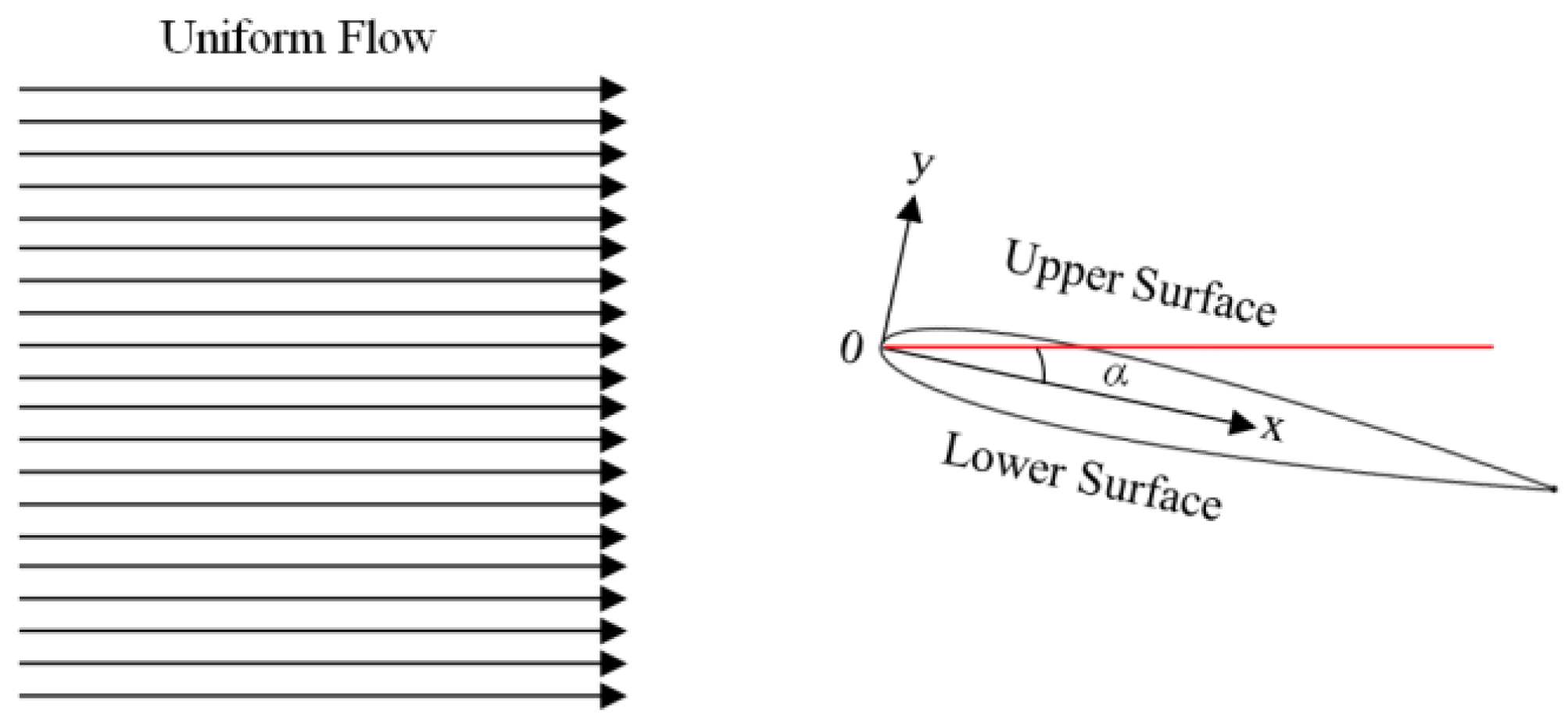
This section presents numerical simulation results for the 2D NACA0012 airfoil at different angles of attack (α) of 6°, 8°, 10°, 12°, 14°, and 16° at Re = 2.88 × 106. These results are compared with wind tunnel experimental results shown by Gregory [31] and others in the literature. Flow conditions around the airfoil at different α values are illustrated in Figure 3.

In the wind tunnel experiments conducted by Gregory [31] and others, the chord length (c) of the NACA0012 airfoil is 760 mm. In this section, numerical simulations for the NACA0012 airfoil are carried out using both the standard k-ω SST turbulence model and the k-ω SST turbulence model corrected using f_c (i.e., the curvature-corrected turbulence model) developed in this study. The comparison of the average lift coefficient (C_L) under different angles of attack with the wind tunnel experimental data from Gregory [31] is presented in

Table 3. Comparison of average lift coefficient (C_L) of NACA0012 at different attack angles.

α (°)	6	8	10	12	14	16
Results of the experiment	0.6801	0.8843	1.0992	1.3000	1.4563	1.5868
Results of standard k-ω SST	0.6471	0.8538	1.05167	1.235925	1.3946	1.5111
Calculation error	−4.9%	−3.4%	−4.3%	−4.9%	−4.2%	−4.8%
Results of k-ω SST corrected using fc	0.6474	0.8539	1.05389	1.239177	1.4020	1.5286
Calculation error	−4.8%	−3.4%	−4.1%	−4.7%	−3.7%	−3.7%

.

The data indicates that although the introduction of the curvature correction factor f_c enhances the prediction of turbulent kinetic energy and improves the simulation accuracy for airfoil flow problems, the degree of improvement remains limited. This is primarily because the flow field variations around the airfoil are relatively mild, and the k-ω SST turbulence model already provides a high accuracy for such cases, particularly in capturing surface-related physical quantities.

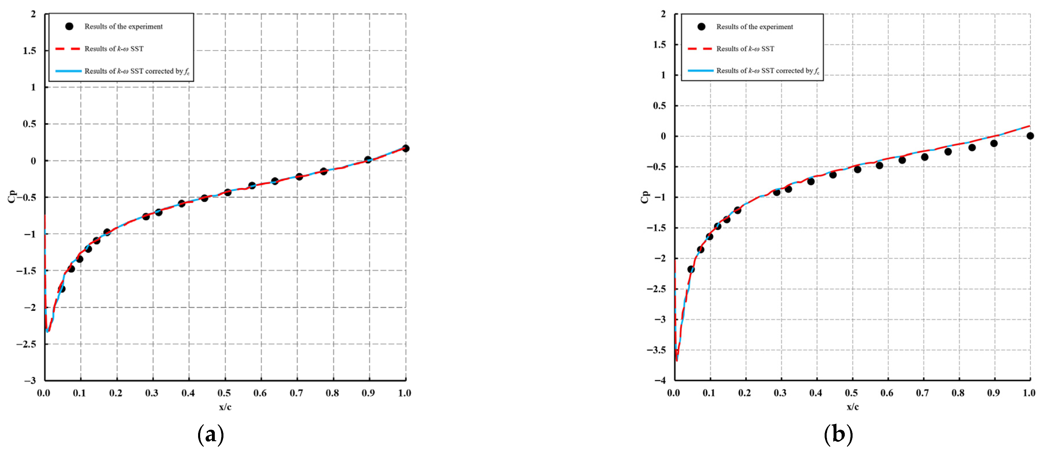
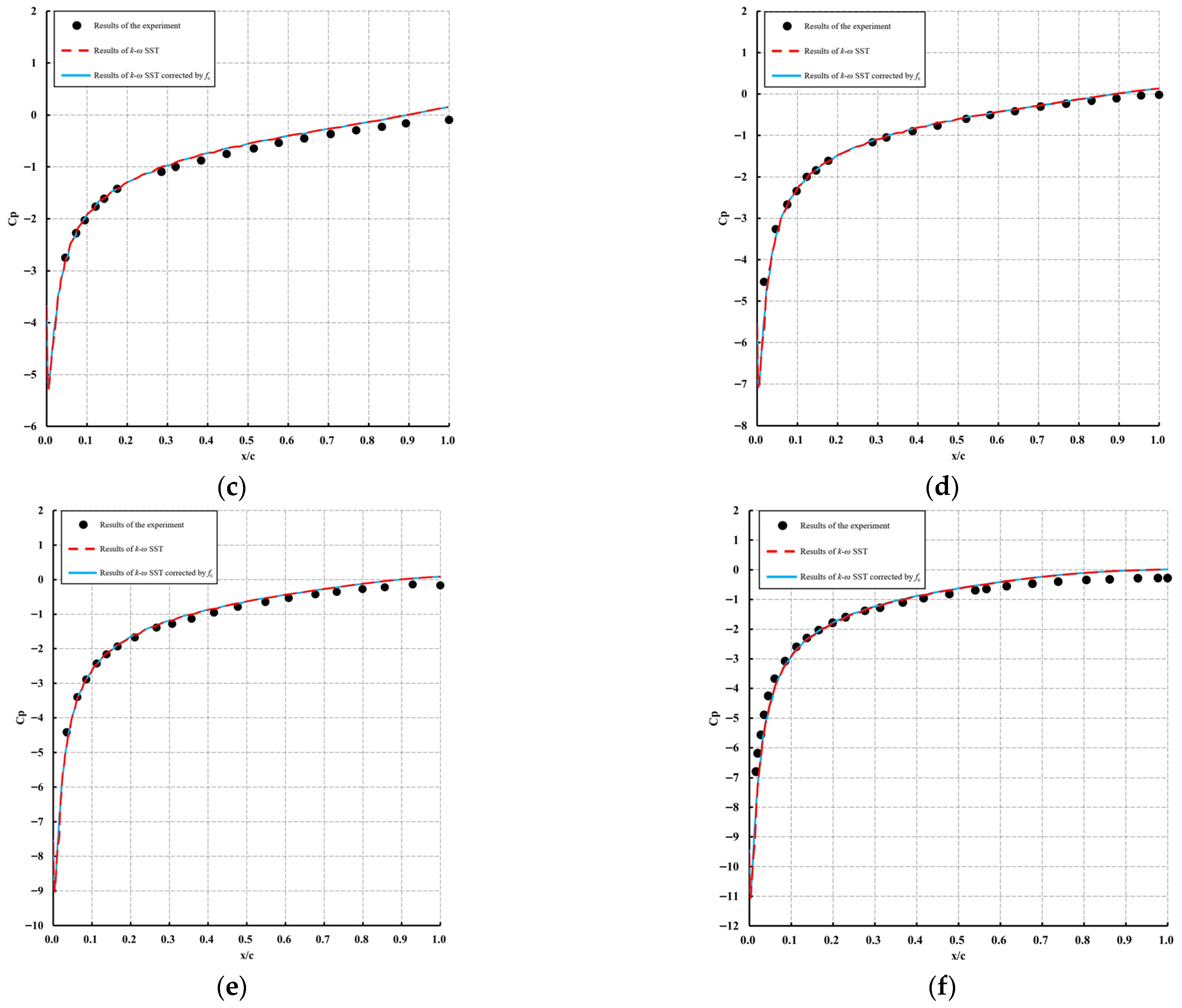
Figure 4 presents the distribution of the time-averaged pressure coefficient (C_P) along the upper surface of the NACA0012 airfoil at various angles of attack. The comparison includes experimental data from Gregory (black solid circles), predictions from the standard k-ω SST turbulence model (blue solid line), and outcomes obtained from the proposed curvature-corrected turbulence model (red solid line). The x-axis denotes the non-dimensional chordwise position, defined as the ratio of the surface coordinate to the chord length c.

As illustrated in Figure 4, the time-averaged pressure coefficient (C_P) distributions obtained using the curvature-corrected turbulence model closely match those predicted by the standard k-ω SST turbulence model and exhibit good agreement with experimental data. This consistency suggests that both turbulence models are capable of accurately capturing the flow characteristics around a two-dimensional airfoil. However, when the x/c is in the range of [0.8, 1], the computed C_P values from both models are slightly lower than the experimental measurements, which may lead to a minor underprediction of the lift coefficient C_L. 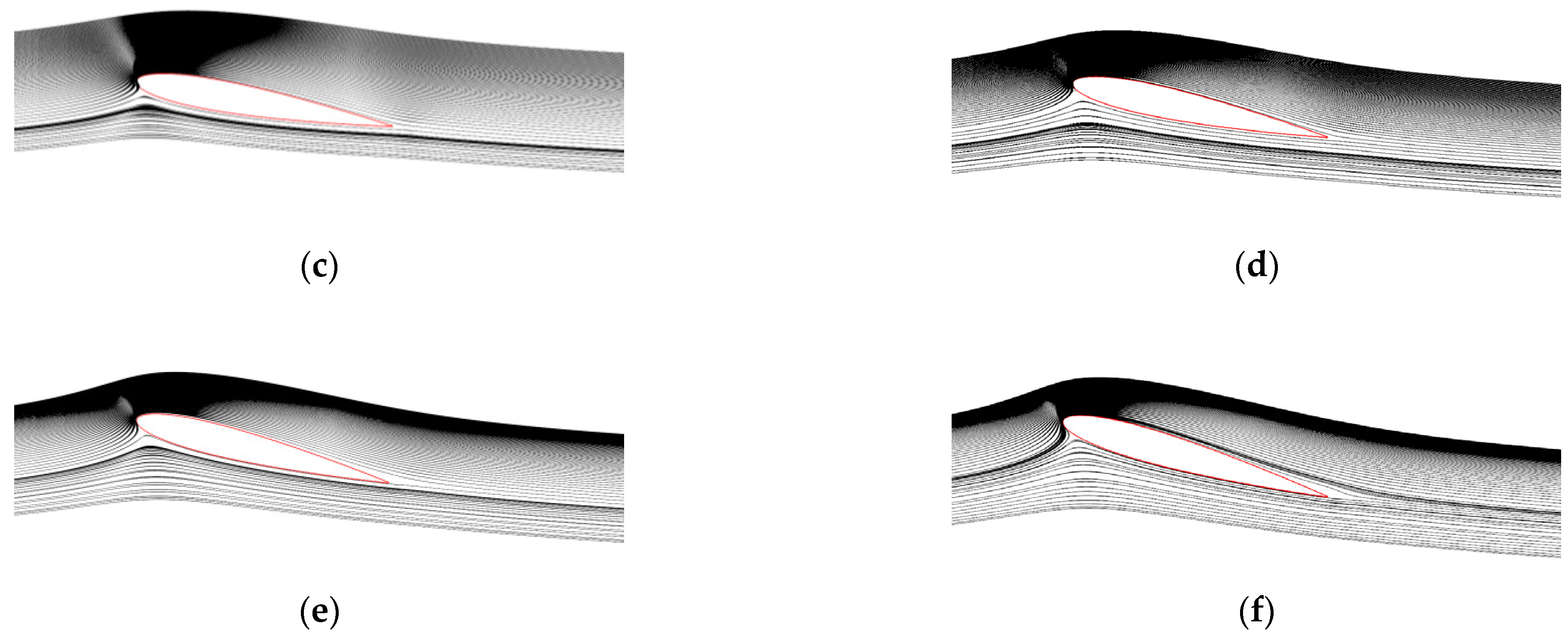Figure 5 presents the streamline patterns around the NACA0012 airfoil at various angles of attack. This case study further confirms that the proposed curvature correction has only a minor effect on non-bluff body flows.

4. Analysis of the Impact of Curvature Correction Factor (${\mathit{f}}_{\mathit{c}}$) on Flow Around a 2D Square Column

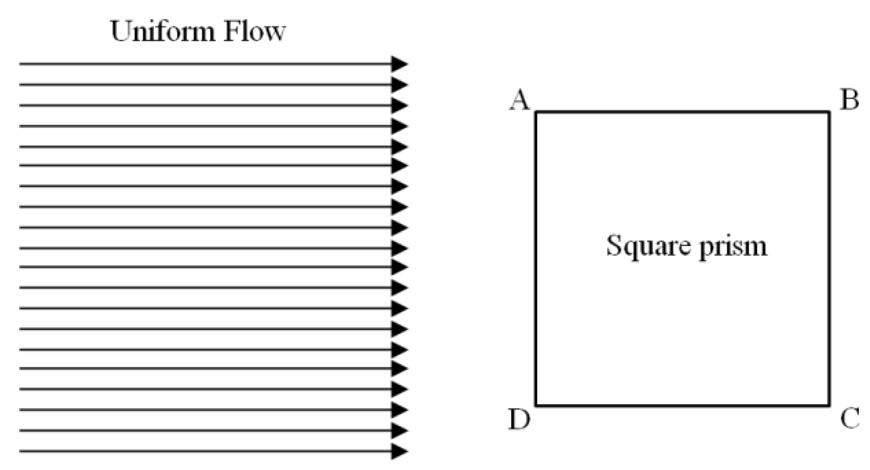
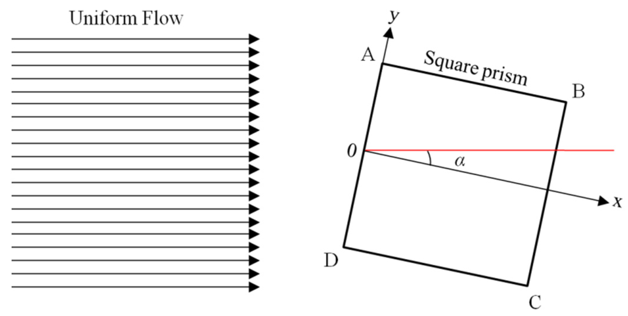
In this section, numerical simulation results for flow past a 2D square column at Re = 1.76 × 10⁵ are presented. These results will be compared with the wind tunnel model experiment results obtained by Lee [18], as documented in the literature. A schematic representation is as show in Figure 6:

To verify the reliability and accuracy of the numerical simulation results, a grid independence analysis was conducted.

Table 4. Steady-state drag coefficient under different cavity boundary grid sizes.

Grid size along cavity boundary (m)	0.00565	0.00400	0.00285	0.00200	0.00125	0.00100	0.00075	0.00050
Steady-state CD coefficient	2.592	2.207	2.611	2.269	2.295	2.231	2.286	2.384

presents the calculated steady-state drag coefficient (C_D) under different grid sizes along the cavity boundary.

The table shows that when the grid size along the boundary is reduced from 0.00565 m to 0.002 m, C_D decreases from 2.59 to 2.27, indicating a noticeable variation. However, when the boundary grid is further refined to 0.001 m or smaller, the variation in C_D becomes significantly smaller, with values stabilized within the range of 2.23–2.39, and the relative error is controlled within 5%. This indicates that the results gradually converge and basically meet the requirements of grid independence.

Considering both numerical accuracy and computational efficiency, this study finally adopted a grid size of 0.02 × 0.05 m along the cavity boundary. This grid ensures stable and reliable results while significantly reducing the computational cost. Therefore, the selected grid system is considered reasonable and reliable.

In the wind tunnel experiments conducted by Lee [18] and others, the square column had a side length of [165 × 165] mm. In this section, numerical simulations for this specific square column are carried out using both the standard k-ω SST turbulence model and the curvature-corrected model developed in this study. The comparison of the mean drag coefficient (C_D) with the wind tunnel experimental data from Lee [18] is presented in

Table 5. The comparison of the mean drag coefficient (C_D).

Results of the Experiment	Results of Standard k-ω SST	Calculation Error	Results of k-ω SST Corrected Using fc	Calculation Error
2.04	2.53	24%	2.21	8.3%

.

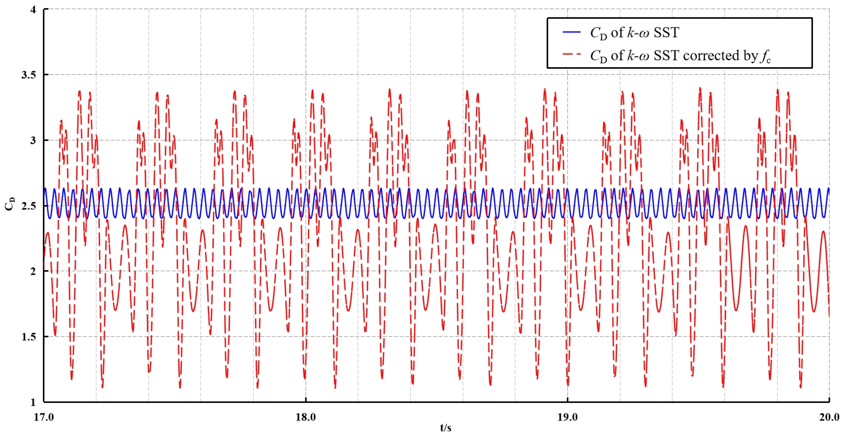
The data clearly shows that for this problem, the curvature-corrected model significantly enhances simulation accuracy. f_c corrects P_k in the transport equation of the k-ω SST turbulence model according to the rotation rate of local fluid mass, which results in a more precise capturing of the vortices formed in the wake as fluid flows around the square column, leading to broader variations in the velocity and pressure fields and consequently, a greater range of C_D variation, as depicted in Figure 7. In this figure, the blue solid line and the red dashed line, respectively, represent the time history curve of C_D from the standard k-ω SST turbulence model and the curvature-corrected turbulence model.

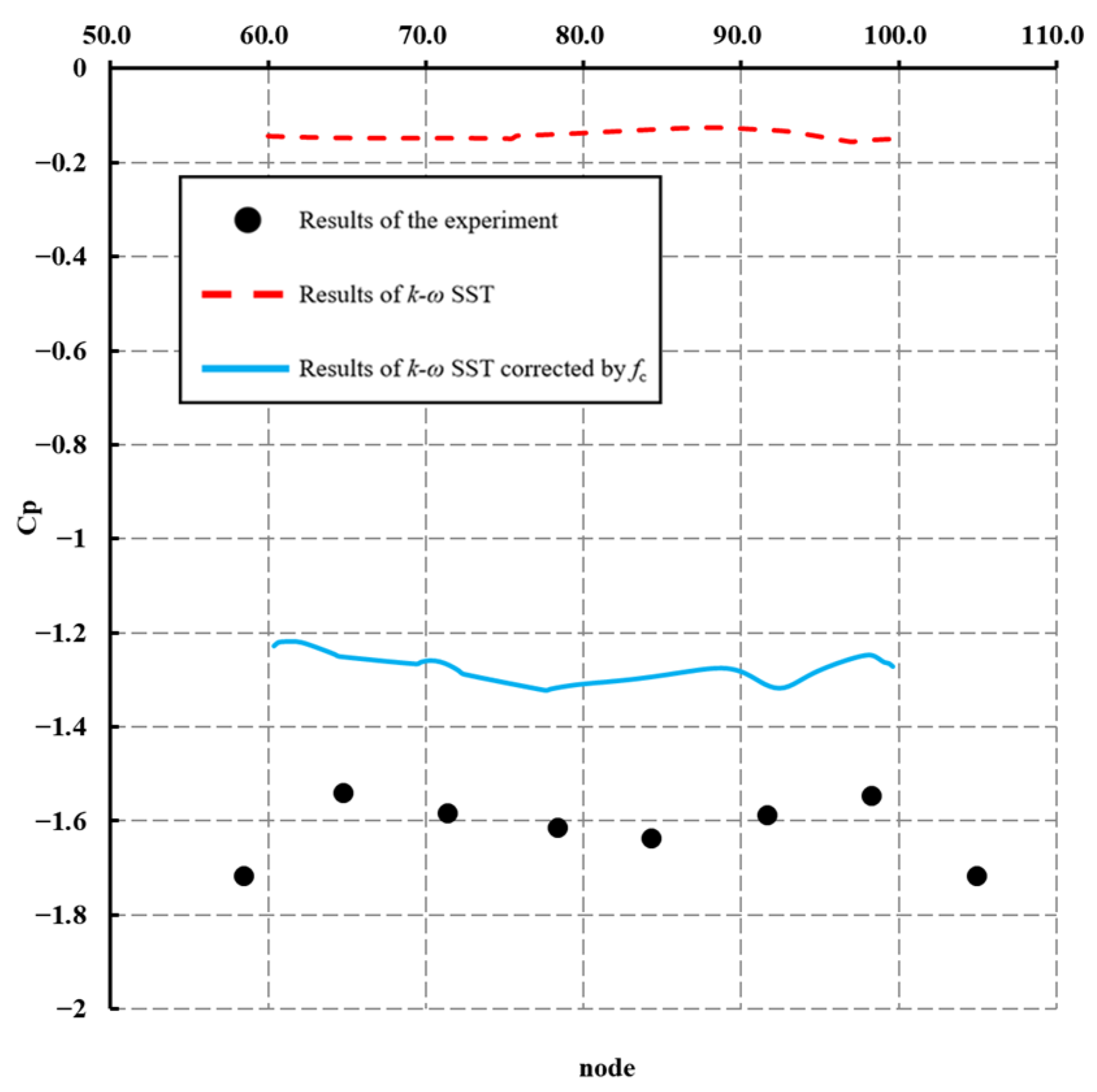
The curvature-corrected turbulence model demonstrates an improved capability in capturing the wake vortices formed downstream of the two-dimensional square column. This results in a more accurate estimation of the pressure coefficient (C_P) along the rear surface (BC edge) of the square column. This improvement is the primary reason why the drag coefficient (C_D) predicted by the curvature-corrected model shows better agreement with experimental results.

Figure 8 presents the C_P distributions obtained from both the standard k-ω SST turbulence model (red dashed line) and the curvature-corrected model (blue solid line), along with experimental data from Lee’s study (black solid circles). The C_P profile predicted by the curvature-corrected model exhibits closer agreement with the experimental results, indicating that the incorporation of the correction factor f_c enhances the accuracy of drag prediction.

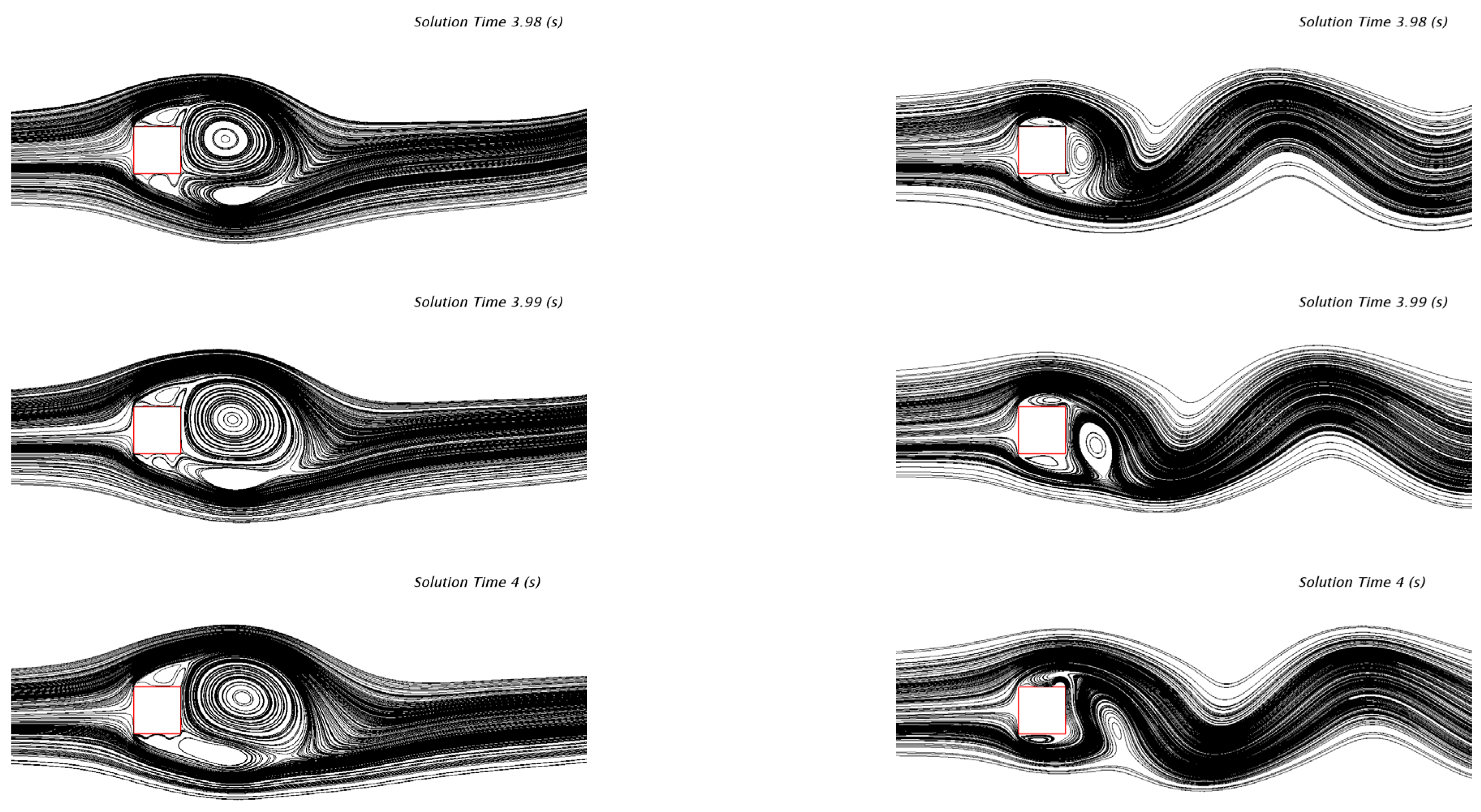
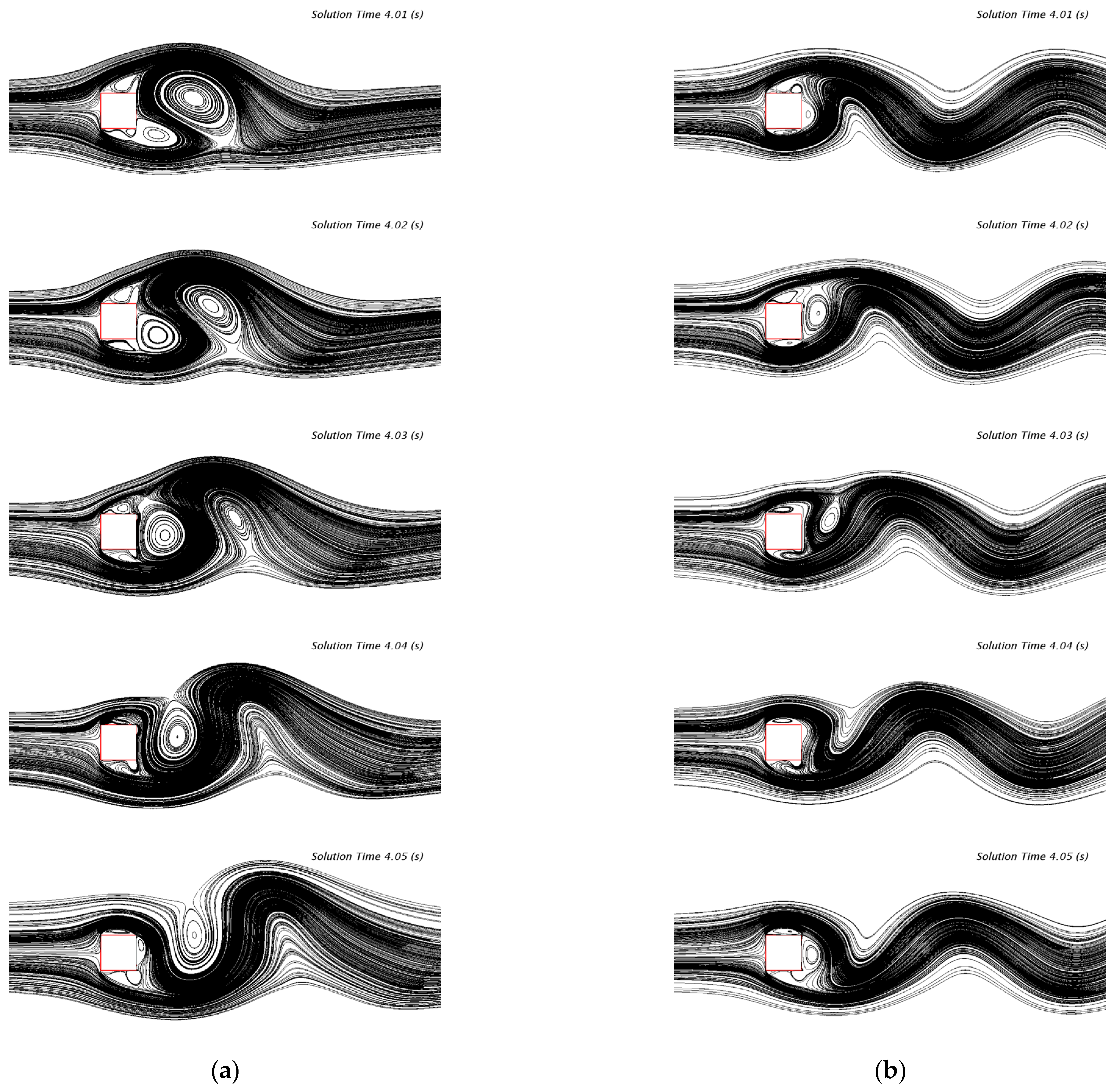
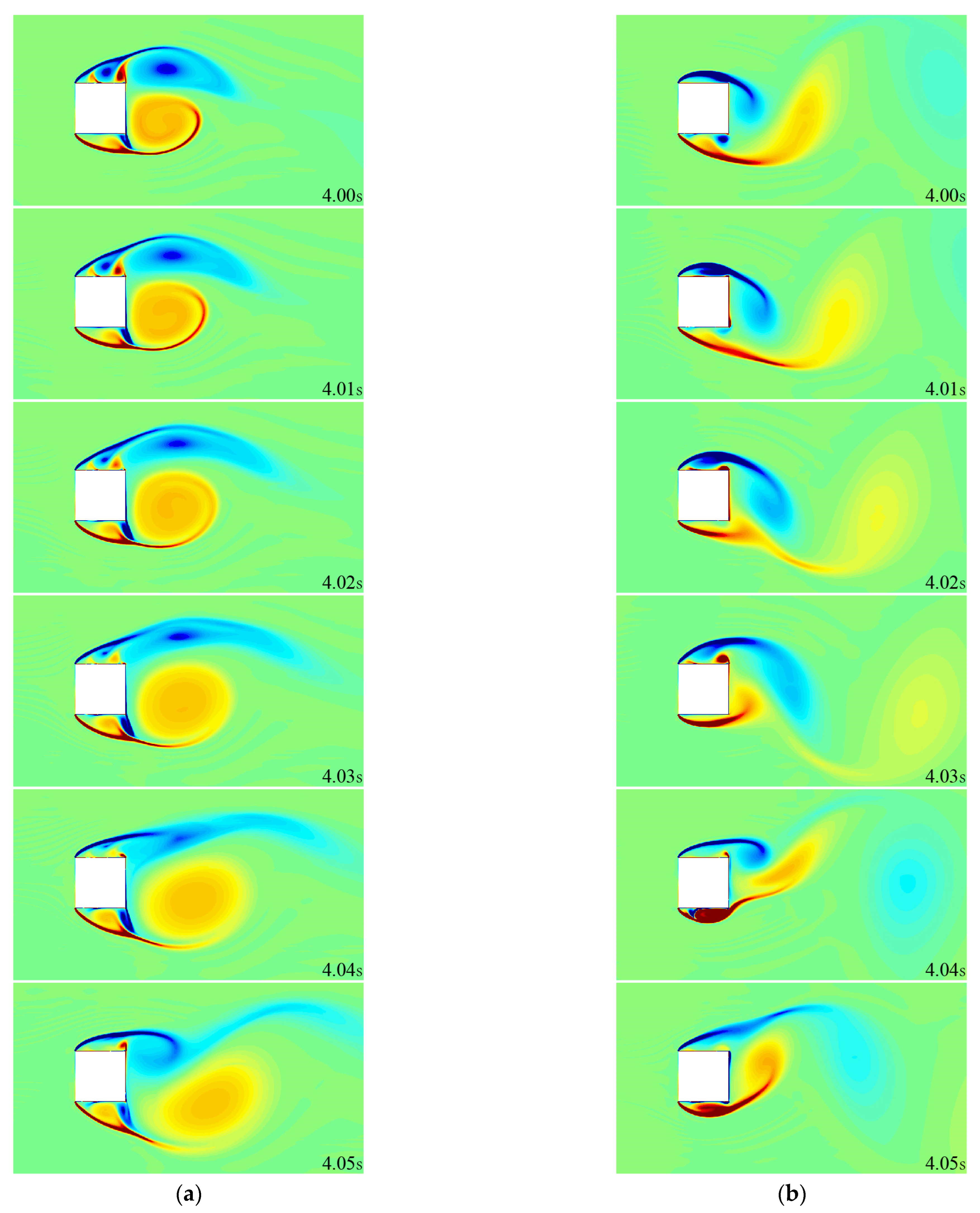
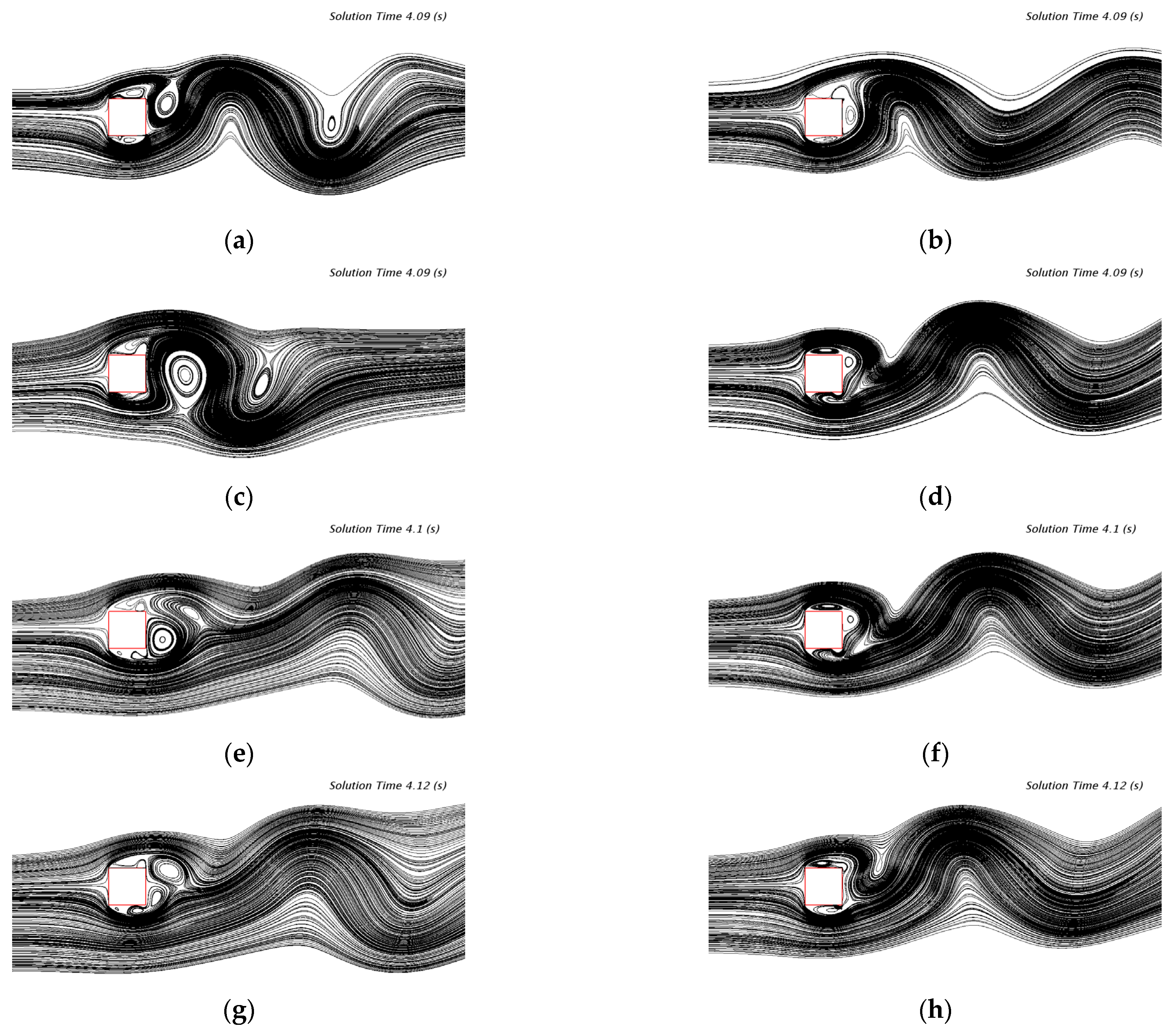
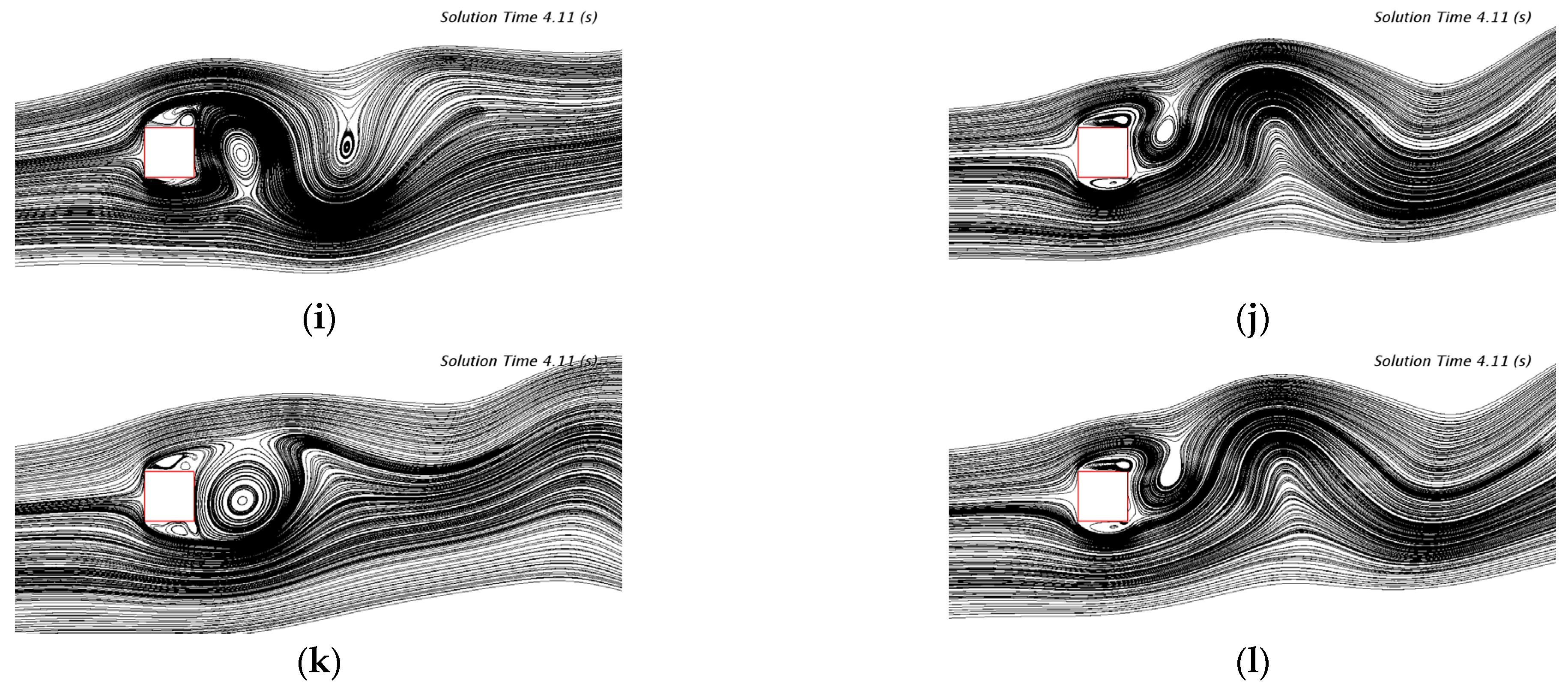
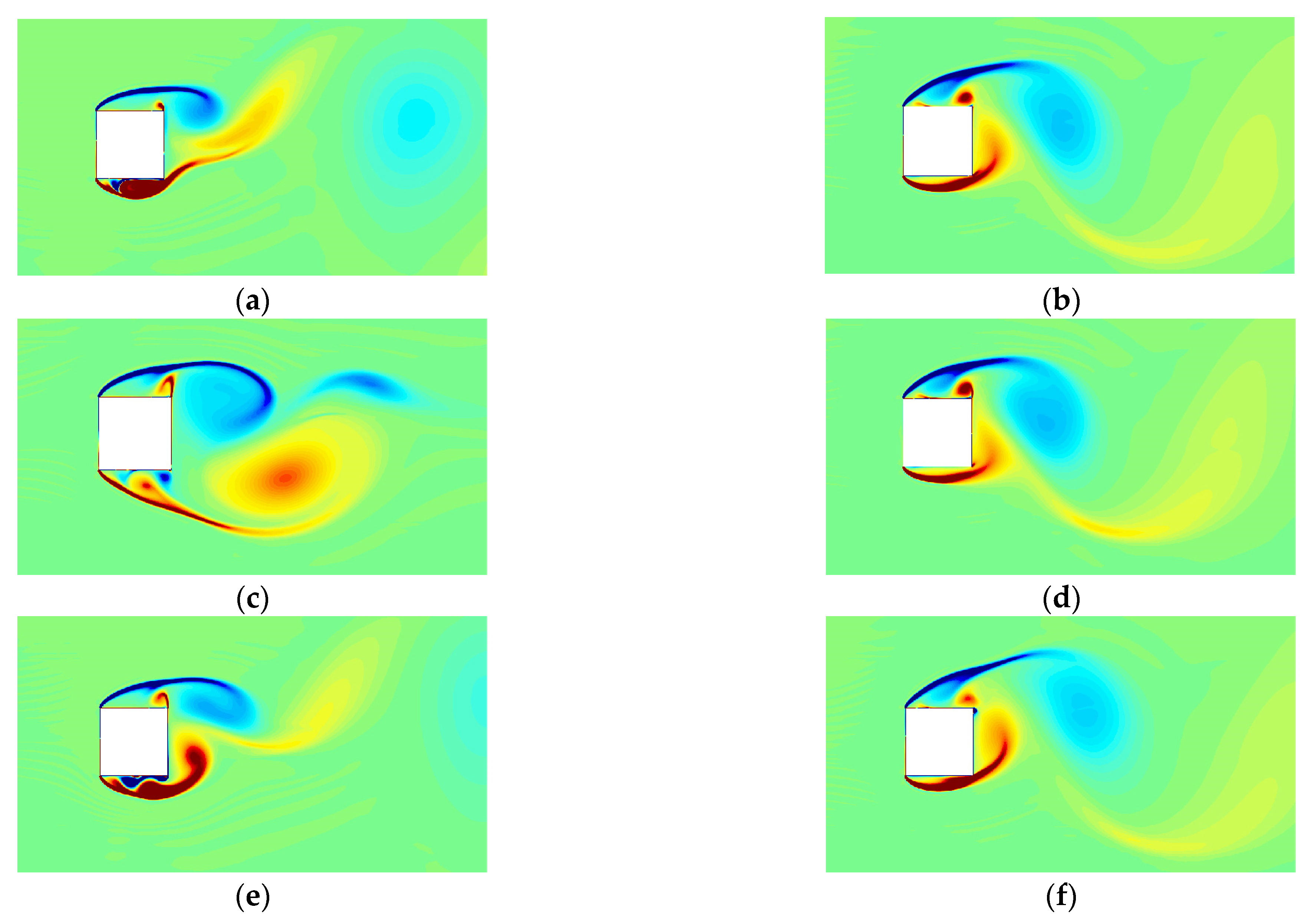
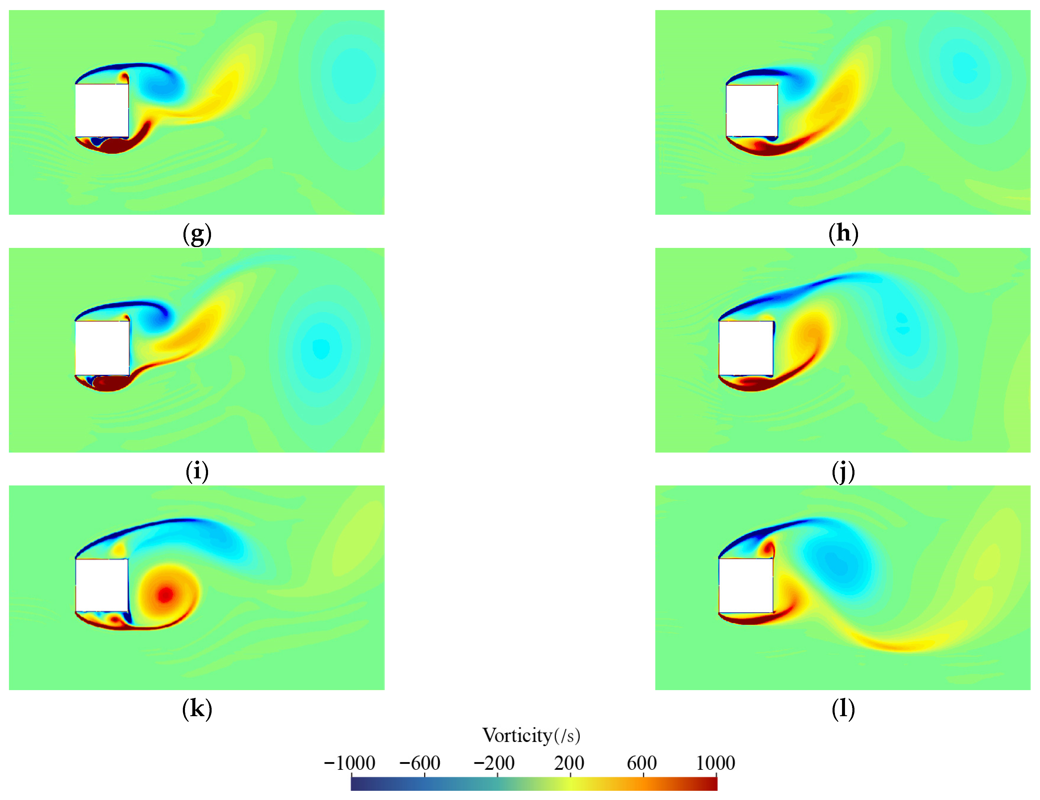
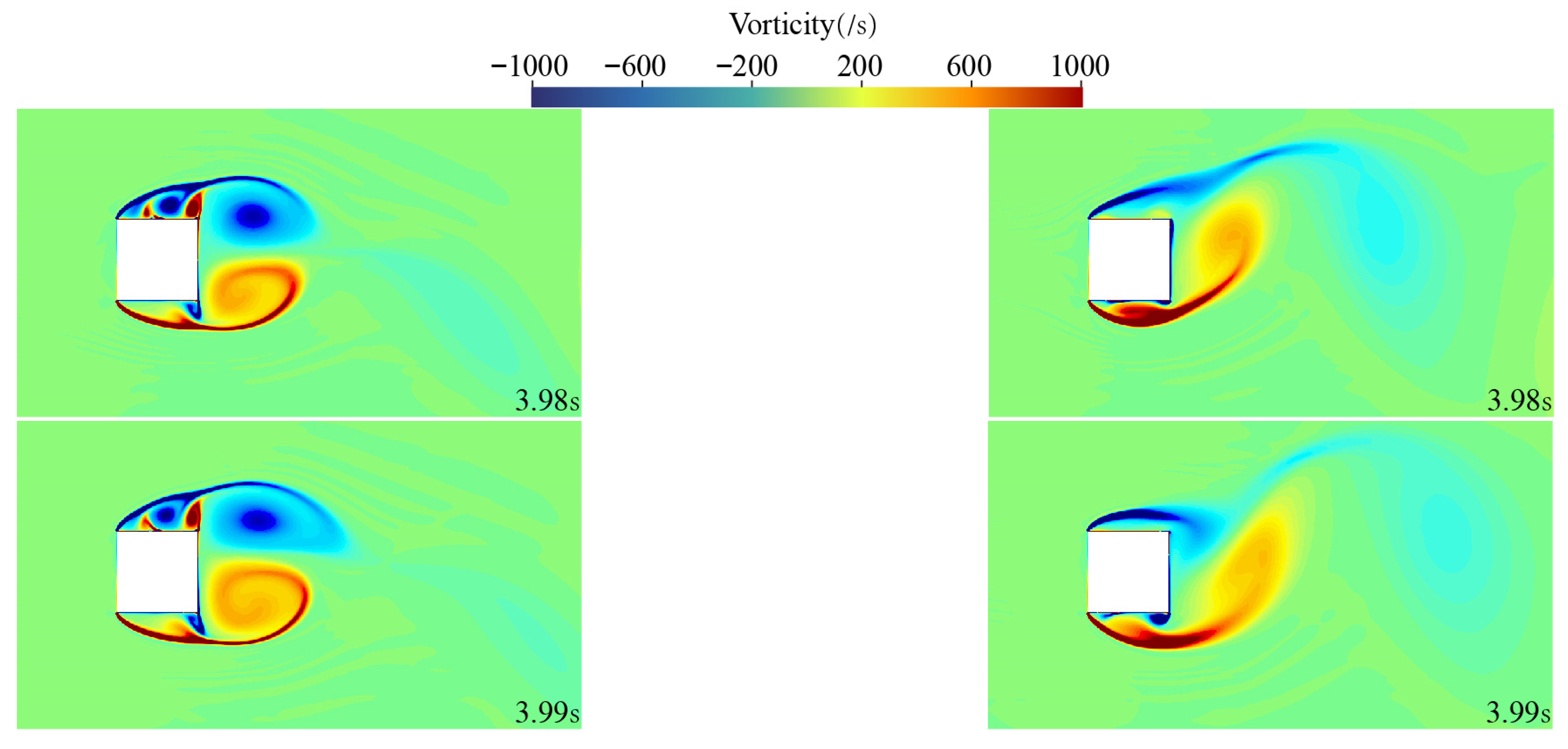
Figure 9 and Figure 10 present the streamline and vorticity distributions obtained using the standard k-ω SST turbulence model and the curvature-corrected turbulence model over the time interval from 3.98 to 4.05 s. The images on the left side represent the flow field calculation results from the curvature-corrected turbulence model, while the images on the right side show the results from the k-ω SST turbulence model. It is evident that the curvature-corrected model has an improved capability in capturing and describing vortex structures, particularly velocity and pressure variations, that better reflect the physical reality. Consequently, the predicted pressure coefficient (C_P) and drag coefficient (C_D) show improved agreement with experimental data.

5. Analysis of the Impact of Curvature Correction Factor ${\mathit{f}}_{\mathit{c}}$ on Flow Around a 2D Square Column at Different Attack Angles

This section presents the numerical simulation results for a 2D square column at α = 1°, 2°, 3°, 4°, 5°, and 6° and Re = 1.76 × 105. The analysis focuses on understanding the influence of f_c on the flow past the square column at different αs. The flow conditions around the square column for each α value are illustrated in Figure 11.

The comparison C_D results under different α values in the k-ω SST turbulence model and the curvature-corrected turbulence model are shown in

Table 6. Comparison of average drag coefficient (C_D) at different attack angles.

α (°)	Results of Standard k-ω SST	Results of k-ω SST Corrected Using fc
1	2.546	2.322
2	2.621	2.364
3	2.619	2.418
4	2.626	2.463
5	2.622	2.505
6	2.625	2.549

. The data indicate that within the range of α = 1–6°, in the k-ω SST turbulence model, the C_D does not change significantly; whereas in the curvature-corrected turbulence model, the C_D increases with α. Furthermore, in the curvature-corrected turbulence model, the C_D is consistently lower than that in the k-ω SST turbulence model for the entire range of α, aligning with the conclusions of the previous section and showing a uniform trend.

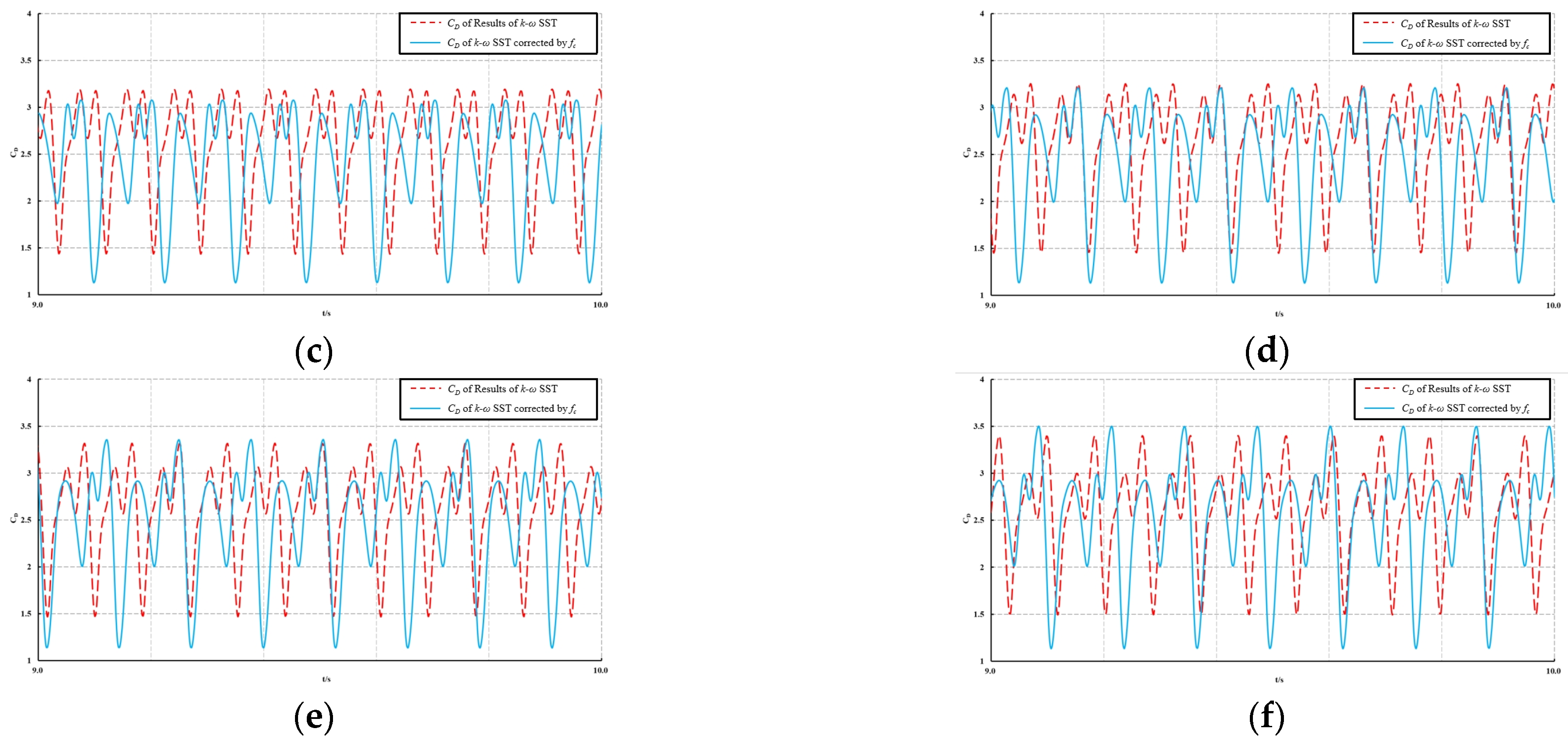
Figure 12 presents the time history curves of the drag coefficient (C_D) at different angles of attack (α) for both the standard k-ω SST turbulence model (blue solid line) and the curvature-corrected turbulence model (red solid line). As α increases, the amplitude of fluctuations in the C_D time history predicted by the standard model also increases, suggesting that larger angles of attack promote the formation of vortices. Under a varying α, the curvature-corrected model consistently captures the wake vortices more accurately, resulting in broader variations in the velocity and pressure fields and a corresponding increase in the fluctuation range of C_D. These findings agree with the conclusions drawn in the previous section.

Figure 13 and Figure 14 illustrate the streamlines and vorticity distribution maps at different α values for both the curvature-corrected turbulence model and the standard k-ω SST turbulence model. In each figure, the left-hand panels show the results obtained from the curvature-corrected model, while the right-hand panels display those from the standard k-ω SST turbulence model.

It can clearly be observed that the curvature-corrected turbulence model has an improved capability in capturing and describing vortex structures across the range of α values, further demonstrating the effectiveness of the correction factor (f_c) in enhancing the original k-ω SST turbulence model’s ability to simulate flow around a two-dimensional square column.

6. Conclusions

Based on the validation studies involving flow past a two-dimensional airfoil and square column, it can be concluded that the k-ω SST curvature-corrected turbulence model referred to in this study modifies the production term P_k. This correction enables more accurate resolution of flow field characteristics and thereby enhances the overall simulation accuracy. The key findings are summarized as follows:

• The impact of f_c on improving the simulation accuracy for flow over two-dimensional airfoils is limited. This is attributed to the relatively weak vorticity generated in such flows, where the rotational motion of fluid particles is not pronounced. In these cases, the standard k-ω SST model already provides satisfactory results.
• The inclusion of f_c significantly improves the simulation accuracy for flow past a two-dimensional square column. For the case with an angle of attack of zero, the simulation error is reduced from 24% (unmodified model) to 8.3% (with curvature correction). For cases with non-zero angles of attack, a similar trend is observed, further validating the robustness and effectiveness of the proposed correction for bluff body flow scenarios.

Future work will extend this study to three-dimensional bluff bodies. Both numerical and experimental investigations will be conducted to assess the applicability and effectiveness of the curvature-corrected model for three-dimensional square column configurations.