A Modified Body Force Model for a Submerged Waterjet

Abstract

The submerged waterjet exhibits advantages such as uniform inflow, minimal flow distortion, and excellent acoustic performance, making it particularly suitable for high-speed vessels. This study investigates the open-water characteristics of the submerged waterjet and develops a body force model for the submerged waterjet propulsion system. First, under uniform inflow conditions, numerical simulations were performed using the body force method by replacing the rotor with a virtual blade and simultaneously replacing both the rotor and stator. The results of the body force model were then compared in detail with those obtained using the sliding mesh method. Second, the influence of the inflow velocity plane position on the results of the body force model was analyzed. The results indicate that the body force method, which replaces both the rotor and stator with a virtual blade, fails to accurately simulate the forces acting on various components of the propeller and the true distribution of the propeller’s flow field. In contrast, the method that replaces only the rotor with a virtual blade produces results for component forces and flow fields that are largely consistent with the results of the sliding mesh method, demonstrating the stability and reliability of the body force model. Additionally, the position of the inflow velocity plane has no significant effect on the model’s computational results.

1. Introduction

Waterjet propulsion has become the preferred propulsion mode for high-speed and high-performance ships due to its advantages of high propulsion efficiency, good anti-cavitation performance, low underwater radiation noise, good maneuverability and no appendages outside the ship suitable for shallow water navigation [1]. Compared with the conventional tail plate waterjet propeller, the submerged waterjet propeller is installed on the bottom plate of the hull stern. The propeller is integrated in the groove at the bottom of the stern, and the nozzle is completely immersed in water. It has the advantages of uniform inflow, small flow deformation and good acoustic performance. In addition, submerged waterjet propulsion combines the characteristics and advantages of conventional propeller propulsion and stern-plate waterjet propulsion. It has important application value and good development potential, and is an important development direction of new propulsion technology for surface ships. Currently, research on waterjet propulsion primarily relies on two approaches: experimental model testing and numerical simulation.

In terms of experimental studies, Gong et al. [2] employed a vehicle-mounted three-dimensional underwater particle image velocimetry (PIV) system to measure the velocity distribution at the intake port during a self-propulsion test of a waterjet-driven ship model in a towing tank. Their findings indicated that the pumping action of the waterjet induced a transverse velocity vector on the cross-section, increasing inflow heterogeneity. Seo et al. [3] conducted a series of model tests to evaluate the performance of waterjet propulsion in a towing tank, including resistance tests, waterjet system tests, and self-propulsion tests, based on a high-speed ship dynamic prediction program.

Despite their reliability, ship model tests have several limitations, including high time and labor requirements, significant costs, constrained experimental conditions, and limited data acquisition capabilities. Computational fluid dynamics (CFD) offers an efficient and cost-effective alternative by enabling full-field flow data acquisition through numerical simulation. Moreover, CFD allows flexible simulation of various operating conditions, effectively overcoming the limitations of traditional experiments and providing more comprehensive technical support for ship design and optimization. With rapid advancements in CFD methodologies and computing power, numerical simulation has become the primary research tool, while model testing is increasingly used for validation purposes. Han et al. [4] numerically predicted the six-degree-of-freedom self-propelled maneuvers of the submarine model BB2 using the CFD method, including steady-state steering maneuvers and space spiral maneuvers. Based on the published test results of the tank model, they verified the effectiveness of the CFD steady-state steering maneuver prediction and conducted the space spiral maneuver prediction on this basis. Ma et al. [5] took the KRISO container ship as the research object, adopted the RANS equation, and respectively used the fluid volume method and the physical force method to study the hydrodynamic characteristics of the model-scale ship and the full-size ship passing through the limited water area at low speed. The results show that the variations of the model and the full-scale vessel in shock force, sway force and yaw moment are basically the same.

Several studies have leveraged CFD to analyze waterjet propulsion systems. Park et al. [6] conducted numerical simulations to investigate the complex three-dimensional viscous flow phenomena, including interactions among the intake duct, rotor, stator, and contraction nozzle. Donyavizadeh et al. [7] discussed the influence of stator blade curvature and thickness on the hydrodynamic performance of a waterjet propeller. Yi et al. [8] conducted resistance and self-propulsion tests on submerged waterjet propulsion ships and used numerical simulations to obtain force distribution data for each component and flow field information. Their results showed strong agreement between computed ship resistance and shaft thrust values and those obtained from experiments, validating the reliability of the numerical approach. Additionally, Cao et al. [9] compared the performance of a single jet pump under uniform inflow conditions with that of a complete jet propulsion system under non-uniform inflow conditions using steady-state simulations. Huang et al. [10] examined the effect of vortex generators on flow separation at the inlet of a waterjet propulsion system, demonstrating that the generators suppressed flow separation along the inlet ramp wall and improved flow uniformity before entering the pump.

Further developments in waterjet propulsion research include novel propulsion configurations and performance enhancements. Yang et al. [11] introduced a new type of waterjet propulsion system centered on a positive displacement pump, comparing its advantages and disadvantages against traditional negative displacement pump systems. Zhao et al. [12] used three-dimensional numerical simulations to study the hydrodynamic characteristics and flow fields of waterjet propulsion under mooring conditions. Cai et al. [13] proposed an integrated propulsion system combining the propeller, power source, and shafting, which was attached to the hull via thrust transmission, and developed a method for measuring thrust in waterjet propulsion. Carlo et al. [14] used computational fluid dynamics (CFD) to study the scale effect of open-water propeller performance. The results showed that the open-water characteristics had a significant scale effect. When the transition model was applied to the numerical simulation of the model scale, the scale effect was significantly reduced. Mikulec et al. [15] presented the verification and validation of full-scale ship trials and CFD simulations. In accordance with industry standards, speed/power trials were conducted under three different power settings. Full-scale unsteady RANS CFD simulations were performed. The results demonstrated good agreement between the numerical predictions and experimental data, confirming the applicability of the numerical method for evaluating full-scale ship performance.

The propeller body force model is an effective approach for evaluating propeller performance. Unlike conventional methods that require detailed geometric modeling and complex rotational motion simulations, the body force method introduces propeller forces as source terms in the momentum equation, simplifying modeling while maintaining high computational efficiency. This method enables accurate prediction of flow field characteristics and is widely applied in propeller propulsion studies. Wu et al. [16] utilized the body force method to predict hull self-propulsion performance, while Fu et al. [17] implemented it for ship self-propulsion calculations at model scale. Hao et al. [18] applied the body force method to simulate ship turning maneuvers. Liu et al. [19] proposed an inside-outflow coupling simulation strategy by integrating lift line theory with the body force method to analyze lift and drag characteristics in an aerodynamic propulsion coupling configuration. Marko et al. [20] introduced a modified body force method that extended its application to azimuth thrusters, addressing the traditional model’s inability to account for lateral forces. Their results demonstrated that the modified approach effectively reproduced force and flow field characteristics while significantly reducing computational workload.

In recent years, with the increasing adoption of waterjet propulsion, research on body force methods for waterjet propulsion systems has expanded. Hino and Ohashi [21] compared and analyzed free-surface variations near the hull of a waterjet-propelled ship under light-body and propeller conditions. They used the body force method to examine the effects of waterjet propulsion and duct structures on the surrounding flow field. Takai et al. [22] applied the body force method to numerically simulate the self-propelled Joint High-Speed Sealift (JHSS) ship. Liu et al. [23] employed the body force method to investigate the influence of waterjets on a waterjet-propelled amphibious ship, comparing the method’s predictions against experimental results and those obtained via the discrete propeller method. Their findings indicated that the body force method achieved higher prediction accuracy. Eslamdoost et al. [24] proposed three different body force models for waterjet propulsors. The first model geometrically removes the impeller and stator blades, applying only the axial forces generated by both the rotor and stator within the body force model. The second model adds tangential forces to the axial forces applied in the first model. The third model replaces only the impeller blades while retaining the stator blades, duct, and other components, applying both the axial and tangential forces generated by the rotor within the body force model. Furthermore, simulations were conducted using methods such as the sliding mesh method and the moving reference frame method. Comparisons of the results from these methods with those from the body force models demonstrated that the third model (retaining the stator and replacing the impeller blades with body forces) provided superior simulation performance. Additionally, compared to the sliding mesh method, the body force method significantly reduced computational time.

The development of a reliable body force model is crucial for the design and performance evaluation of submerged propulsion systems. While previous studies have primarily focused on applying the body force method to simulate ship self-propulsion, research on the construction and application of body force models specifically for waterjet propellers remains limited. In this study, a series of numerical investigations on a submerged waterjet propeller are conducted using CFD. An uncertainty analysis is performed to validate the numerical methodology. By analyzing the open-water characteristics of submerged jet propulsion, a body force model tailored to submerged waterjet propulsion systems is developed. Additionally, the influence of inflow velocity plane position on the model’s results is examined. The reliability of the proposed body force model is validated by comparing its results with those obtained from the sliding mesh method under uniform flow conditions.

2. Geometries Studied

To validate the research methodology, a type of propeller suitable for a submerged waterjet propulsion ship is employed, which is composed of duct, rotor and rear stator. The number of rotor blades is 5, and the number of rear stator blades is 7. The geometry model of the propeller is shown in Figure 1, the main parameters are shown in

Table 1. Main parameters of the waterjet propeller.

Main Parameter	Symbol	Units	Value
Diameter of the rotor	$D_R$	m	0.166
Diameter of the Hub	$D_{Shaft}$	m	0.021
Hub diameter ratio	$D_R/D_{Shaft}$	-	0.25
Length of the duct	$L_D$	m	0.251
Inlet diameter	$D_1$	m	0.174
Outlet diameter	$D_2$	m	0.164
Blades number of rotor	$N_D$	-	5
Blades number of stator	$N_R$	-	7
Rotation direction	-	-	Right-handed

.

3. Computational Method

3.1. Governing Equation and Turbulence Model

In this study, numerical simulations of incompressible viscous flow are performed using star ccm+ 202302.0001. The CFD method is used to solve the unsteady RANS equations to simulate the flow characteristics of a submerged waterjet propulsion system. The governing equations of the URANS method are expressed as follows:

$${\displaystyle \frac{\mathsf{\partial }{(U}_i)}{\mathsf{\partial }{x}_i}}=0$$

(1)

$${\displaystyle \frac{\mathsf{\partial }{U}_i}{\mathsf{\partial }t}}+U_j{\displaystyle \frac{\mathsf{\partial }{U}_i}{\mathsf{\partial }{x}_j}}=-{\displaystyle \frac{1}{\rho }}{\displaystyle \frac{\mathsf{\partial }p}{\mathsf{\partial }{x}_i}}+{\displaystyle \frac{1}{\rho }}{\displaystyle \frac{\mathsf{\partial }}{\mathsf{\partial }{x}_j}}\left(\mu {\displaystyle \frac{\mathsf{\partial }{U}_i}{\mathsf{\partial }{x}_j}}-\rho \overline{u_i{u}_j}\right)$$

(2)

where $U_i$ (i = 1, 2, 3) is the time-averaged velocity component and $u_i$ (i = 1, 2, 3) refers to the fluctuation velocity component; $\rho$ is the density; P is the time-averaged pressure; $\mu$ is the dynamic viscosity; and $\rho \overline{u_i{u}_j}$ is the Reynolds stress term.

To achieve turbulence closure, the shear-stress transport (SST) k-ω turbulence model, originally proposed by Menter [25], is employed.

The SST k-ω model enhances the accuracy of flow separation prediction and is well-suited for resolving complex flow fields. In the numerical simulations, a pressure-based coupling approach is employed for solving the governing equations. The convective terms are discretized using a second-order upwind scheme to enhance numerical stability and accuracy, while the diffusive terms are discretized using a second-order central difference scheme.

3.2. Body Force Model

The body force method is a special model that simulates the motion of a thruster, without real geometry, by adding the model at grid points within a given range to output force and torque. The application of the body force method can change the rotational motion of propeller from unsteady state to steady state. In addition, there is no need to divide the grid according to the real geometry, which greatly reduces the requirements on the mesh quantity and time step in the numerical simulation, greatly improves the computing speed and saves computing resources.

The body force method is designed to model the thrust, torque and other effects of the rotating part of the propeller, and it is not necessary to directly solve the motion of the actual rotating part. The application range of the body force region is a cylinder. This method distributes the body force $f_b$ axially in the cylinder region, and follows a certain distribution in the radial direction. The distribution of force in this paper adopts Goldstein optimal distribution, and the relevant formulas are as follows:

$$f_{bx}=A_x{r}^{*}\sqrt{1-r^{*}}$$

(3)

$$f_{b\theta }=A_{\theta }·{\displaystyle \frac{r^{*}\sqrt{1-r^{*}}}{r^{*}\left(1-r_h^{\prime }\right)+r_h^{\prime }}}$$

(4)

$$r^{*}={\displaystyle \frac{{r^{\prime }-r}_h^{\prime }}{1-r_h^{\prime }}}, r_h^{\prime }={\displaystyle \frac{R_H}{R_P}},r^{\prime }={\displaystyle \frac{r}{R_P}}$$

(5)

where $f_{bx}$ and $f_{b\theta }$ represent the axial and tangential components of the body force, respectively. r is the radial coordinate; $R_H$ is the radius of the hub; $R_P$ indicates the radius of the tip circle. $A_x$ and $A_{\theta }$ are constants, which can be defined as follows:

$$A_x={\displaystyle \frac{105}{8}}·{\displaystyle \frac{T}{\pi ∆\left(3R_H+4R_P\right)\left(R_P-R_H\right)}}$$

(6)

$$A_{\theta }={\displaystyle \frac{105}{8}}·{\displaystyle \frac{Q}{\pi ∆R_P\left(3R_H+4R_P\right)\left(R_P-R_H\right)}}$$

(7)

where $T$ is propeller thrust; $Q$ represents propeller torque; $∆$ indicates the thickness of the body force virtual disk.

3.3. Computational Domain and Boundary Condition

An appropriate computational domain measuring 15$D_R$ (length) × 6$D_R$ (diameter) is created for the propeller open-water simulations, the boundary conditions are shown in Figure 2. The velocity inlet is 5$D_R$ upstream from the center of the rotor, and the pressure outlet is 10$D_R$ downstream from the center of the rotor. The side of the computational domain is set as a symmetrical plane; the propeller surface is defined as a non-slip wall.

The grid of the propeller open-water calculation is shown in Figure 3. To accurately simulate the flow field information during the rotation of the propeller rotor and meet the requirements of the selected turbulence model, the thickness of the near-wall mesh is set to 1.45 × 10⁻⁵ m, the number of boundary layers is not less than 16, as shown in Figure 3. The dimensionless wall distance Y+ distribution on the propeller surface is generally less than 1. The grid distribution is shown in Figure 4.

3.4. Numerical Validation

To verify the accuracy and reliability of the numerical method, based on the public test data, the uncertainty analysis is carried out by using the safety factor method proposed by Xing and Stern [26]. According to the regulations recommended by ITTC [27], the uncertainty of CFD numerical calculation can be expressed as

$$U_{SN}=\sqrt{{U_G}^2+{U_T}^2+{U_O}^2}$$

(8)

where $U_G$ is the grid uncertainty; $U_T$ is the time step uncertainty; and $U_O$ represents the uncertainty caused by other factors, which can be ignored in subsequent analysis.

The refinement ratio $r_k$ between solutions is assumed as

$$r_k={\displaystyle \frac{∆x_2}{∆x_1}}={\displaystyle \frac{∆x_3}{∆x_2}}$$

(9)

where $∆x_i$ (i = 1, 2, and 3) are the coarse, medium, and fine grids or time steps, respectively.

According to the ITTC recommended procedures for uncertainty analysis in simulation calculations, the convergence coefficients $R_k$ (k = G denotes grid and k = T denotes time step) are used to assess the convergence of grid and time step settings. The convergence factor $R_k$ is defined as follows:

$$R_k={\displaystyle \frac{{\epsilon }_{32}}{{\epsilon }_{21}}}$$

(10)

where ${\epsilon }_{21}={\widehat{S}}_m$ – ${\widehat{S}}_c$, ${\epsilon }_{32}={\widehat{S}}_f$ – ${\widehat{S}}_m$; ${\widehat{S}}_f$, ${\widehat{S}}_m$, ${\widehat{S}}_c$ refer to the results of fine, medium and coarse, respectively.

Based on the convergence factor $R_k$ for grid or time step, the convergence can be determined.

(1) $0<R_k<1$ Monotonic convergence (MC).

(2) $-1<R_k<0$ Oscillatory convergence (OC).

(3) $\left|R_k\right|>1$ Divergence.

To conduct prediction analysis and validation of the hydrodynamic performance of a certain type of waterjet propulsion unit designed by the MARIC (Marine Design and Research Institute of China). The propulsion unit consists of a duct, a rotor, and a post-stator; the rotor has 6 blades, and the post-stator has 8 blades, with its geometric model shown in Figure 5.

Before conducting the waterjet simulations, the present numerical method has been verified and validated. In this study, the thrust coefficient for the propeller model is analyzed. The following coefficients are defined:

Advance coefficient:

$$J={\displaystyle \frac{V}{nD}}$$

(11)

Thrust and torque coefficient:

$$K_T={\displaystyle \frac{T}{\rho n^2{D}^4}}$$

(12)

where V is the inflow velocity, n is the rotation speed, and T is the thrust.

The rotor thrust coefficient is $K_T$ when the advance coefficient J = 0.8 is selected for numerical uncertainty analysis and calculation. The numerical results were compared with experimental fluid dynamics (EFD) data for the waterjet propeller, as presented in

Table 2. Uncertainty analysis of a waterjet propeller.

	Grids Number (Million)	${\mathit{K}}_{\mathit{T}}$	Error (%)	Time Step (s)	${\mathit{K}}_{\mathit{T}}$	Error (%)
EFD	-	0.5608	-	-	0.5608	-
${\widehat{S}}_f$	11.891	0.5590	−0.32	1.26 × 10−4	0.5601	−0.12
${\widehat{S}}_m$	8.696	0.5574	−0.61	2.53 × 10−4	0.5574	−0.61
${\widehat{S}}_c$	6.537	0.5550	−1.03	5.05 × 10−4	0.5512	−1.70
$R_k$	-	0.6974	-	-	0.4487	-
Convergence		MC			MC

.

As shown in Table 2. The grid density and time step independence verification for $K_T$ of the propulsor both showed monotonic convergence. The simulation results obtained using a medium grid size and a medium time step exhibited an error of −0.61% compared to the EFD data, which is within the numerical uncertainty range. This further validates the reliability of the numerical method employed in this study for predicting the hydrodynamic performance of the propeller.

For the submerged waterjet propeller studied in this paper, the advance coefficient J = 1.1 and rotational speed $n$ = 16 rps are selected, with the thrust coefficient $K_T$ as the target value for conducting sensitivity analyses of grid and time step size. A grid refinement ratio $r_k=\sqrt{2}$ and a time step refinement ratio $r_k=\sqrt{2}$ are chosen to estimate numerical uncertainty. The coarse, medium, and fine grids consist of 4.756 million, 6.432 million, and 8.706 million grid nodes, respectively. Time steps are set to 0.000694, 0.000347 and 0.000174 s, corresponding to 4, 2 and 1 degrees of propeller rotation per time step, respectively. The calculation results are shown in

Table 3. Uncertainty analysis of waterjet propeller.

	Grids Number (Million)	KT	Error (%)	Time Step (s)	KT	Error (%)
Coarse	4.756	0.2968	1.55	0.000694	0.2958	1.23
Medium	6.435	0.2922	-	0.000347	0.2922	-
Fine	8.706	0.2897	−0.87	0.000174	0.2991	−0.11

.

The sensitivity analysis of grid and time step size is shown in Table 3. The computational results from three different grid density schemes and three different time step schemes demonstrate good convergence, further indicating the reliability of the numerical method used in this study for predicting the hydrodynamic performance of the propulsor. Considering both computational accuracy and cost, the medium grid size and medium time step configuration are selected for subsequent calculations.

4. Construction of Body Force Model

4.1. Open-Water Characteristics of the Discretized Propeller

To analyze the hydrodynamic performance of the propeller, the sliding mesh method was employed to predict its hydrodynamic characteristics. This method requires direct grid discretization of the rotor geometry, allowing for an accurate representation of both the rotor’s shape and its actual motion in the numerical simulation. Consequently, it effectively captures the real flow conditions within the flow channel.

The hydrodynamic simulation of the propeller was conducted using a fixed rotational speed approach while varying the incoming flow velocity. In this study, the propeller operated at a constant speed of n = 16 rps, with the incoming flow velocity $V_A$ ranging from 0.2656 m/s to 3.4528 m/s. The time step for the rotor’s rotational simulation was set to 0.000347 s, corresponding to a 2° rotation per time step at 16 rps.

The open-water performance results of the propeller are presented in Figure 6, where $J$ represents the advance coefficient; $K_{TR}$ is the rotor thrust coefficient; $K_{TA}$ is the combined rotor and stator thrust coefficient; $K_Q$ is the torque coefficient; and $\eta$ denotes the propeller efficiency, defined as

$$J={\displaystyle \frac{V_A}{n{D}_R}}$$

(13)

$$K_{TR}={\displaystyle \frac{T_R}{\rho n^2{D}_R^4}}$$

(14)

$$K_{TA}={\displaystyle \frac{T_R+T_S}{\rho n^2{D}_R^4}}$$

(15)

$$K_Q={\displaystyle \frac{Q}{\rho n^2{D}_R^5}}$$

(16)

$$\eta ={\displaystyle \frac{J{K}_T}{2\pi K_Q}}$$

(17)

where $T_R$ is the thrust of propeller rotor, $T_S$ is the stator thrust, $\rho$ represents the fluid density, $Q$ is torque, and rotor and stator thrust $T_A$ = $T_R+T_S$.

4.2. Body Force Method

When constructing the body force model, the actual geometric structure of the propeller components does not need to be considered. Instead, the body force is assumed to be uniformly distributed along the axial direction on a virtual cylindrical disk. In this study, based on the open water results calculated by the sliding mesh method, a modified body force method is employed to analyze two scenarios: replacing only the rotor, and replacing both the rotor and stator.

The inlet section of the propeller duct is selected as the inflow velocity plane for the body force method. The incoming flow velocity $V_A$ is corrected using the average flow velocity at the inlet of the propeller duct, $V_{inlet}$, to refine the open-water curve. The corrected advance coefficient, $J_{inlet}$, is defined as

$$J_{inlet}={\displaystyle \frac{V_{inlet}}{n{D}_R}}$$

(18)

where n is the rotational speed and $D_R$ is the rotor diameter.

Figure 7 presents the average velocity distribution across the inlet section of the duct at different inflow velocities, while the modified open-water characteristic curve is shown in Figure 8.

5. Verification for the Results

5.1. Body Force Method Replaces Rotor Geometry

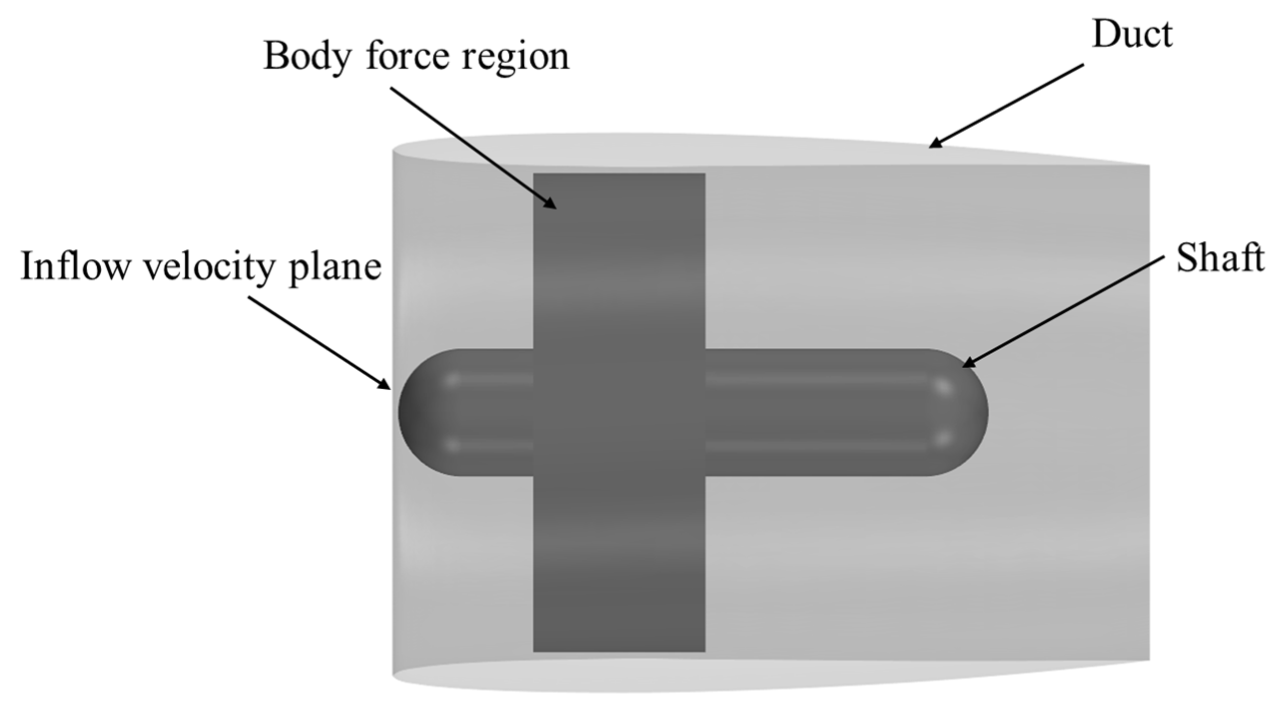
The rotor blade is replaced (referred to as AD-R) using the modified body force method described earlier, while keeping the shafting, stator blades, and duct intact. As shown in Figure 9, the applied body force region is modeled as a cylinder, where its diameter corresponds to the rotor blade diameter, and its thickness is the axial length of the rotor blade. The input for the body force method consists of ${J_{inlet}\text{-}K}_{TR}$ and ${J_{inlet}\text{-}K}_Q$. The section at the inlet of the propeller duct is selected as the inflow velocity plane for AD-R.

For the simulation of the replacement rotor blade, the fixed body force speed $n$ = 16 rps is consistent with the simulation of the sliding mesh method, with different flow speeds varied within the range of 1.062 m/s to 3.4528 m/s. The comparison of the thrust coefficient and torque coefficient of the propeller rotor calculated by AD-R and the sliding mesh method is presented in

Table 4. Comparison of propeller performance between the sliding mesh method and AD-R.

${\mathit{V}}_{\mathit{A}}$ (m/s)	${\mathit{K}}_{\mathit{T}\mathit{R}1}$	${\mathit{K}}_{\mathit{T}\mathit{R}0}$	δ (%)	$10{\mathit{K}}_{\mathit{Q}1}$	$10{\mathit{K}}_{\mathit{Q}0}$	δ (%)
1.0624	0.5745	0.5646	1.754	1.5419	1.5283	0.889
1.3280	0.5360	0.5280	1.525	1.4604	1.4489	0.790
1.5936	0.5054	0.4903	3.094	1.3952	1.3661	2.129
1.8592	0.4632	0.4530	2.243	1.3048	1.2839	1.626
2.1248	0.4210	0.4146	1.548	1.2140	1.1983	1.311
2.3904	0.3763	0.3760	0.070	1.1169	1.1137	0.289
2.6560	0.3298	0.3352	−1.606	1.0149	1.0239	−0.878
2.9216	0.2823	0.2922	−3.410	0.9087	0.9296	−2.249
3.1872	0.2353	0.2465	−4.523	0.8011	0.8276	−3.194
3.4528	0.1921	0.1981	−3.043	0.6977	0.7178	−2.804

. Here, the numerical simulation results of the sliding mesh method are represented by subscript 0, the numerical simulation results of AD-R are represented by subscript 1, δ represents the parameter change rate of the former relative to the latter.

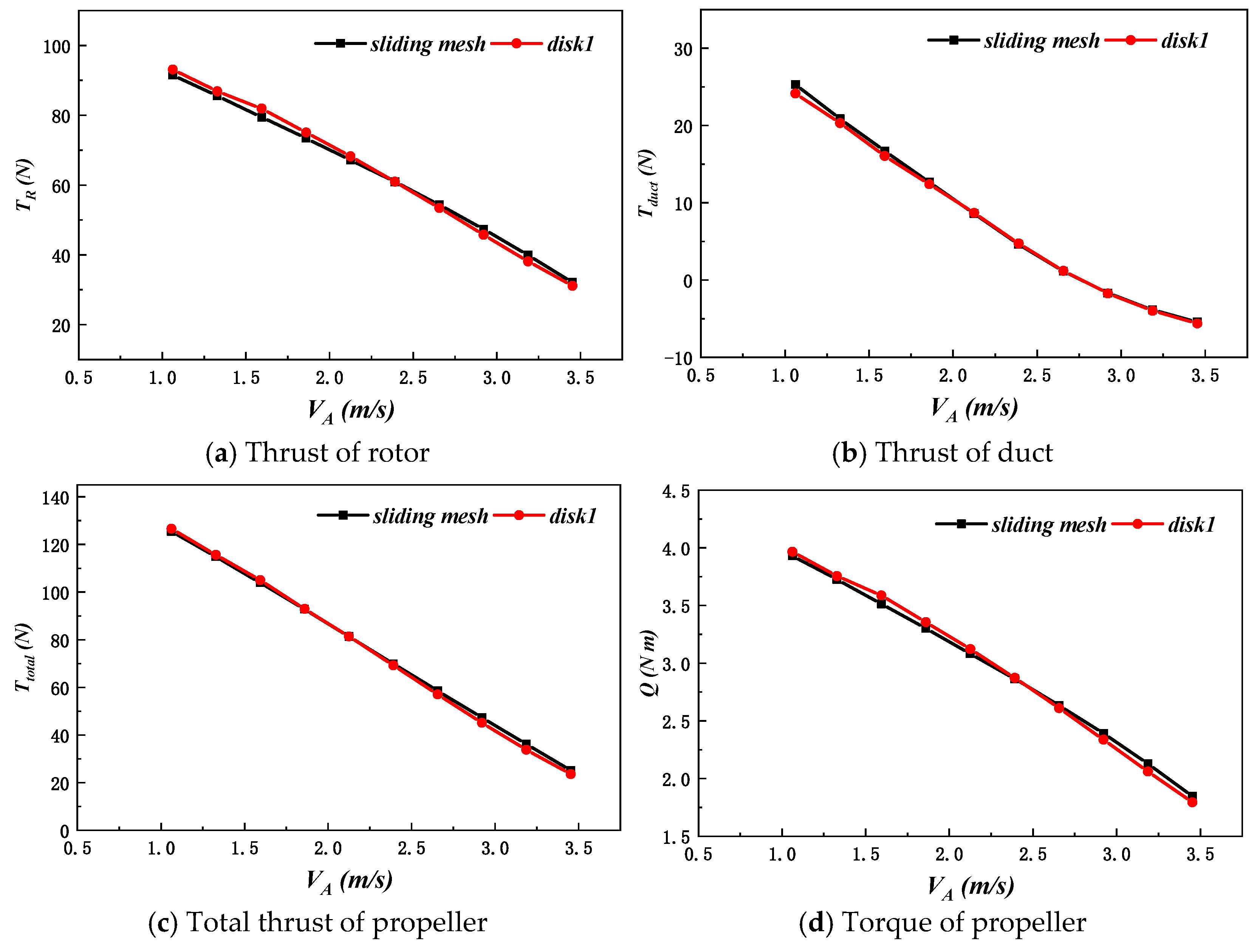
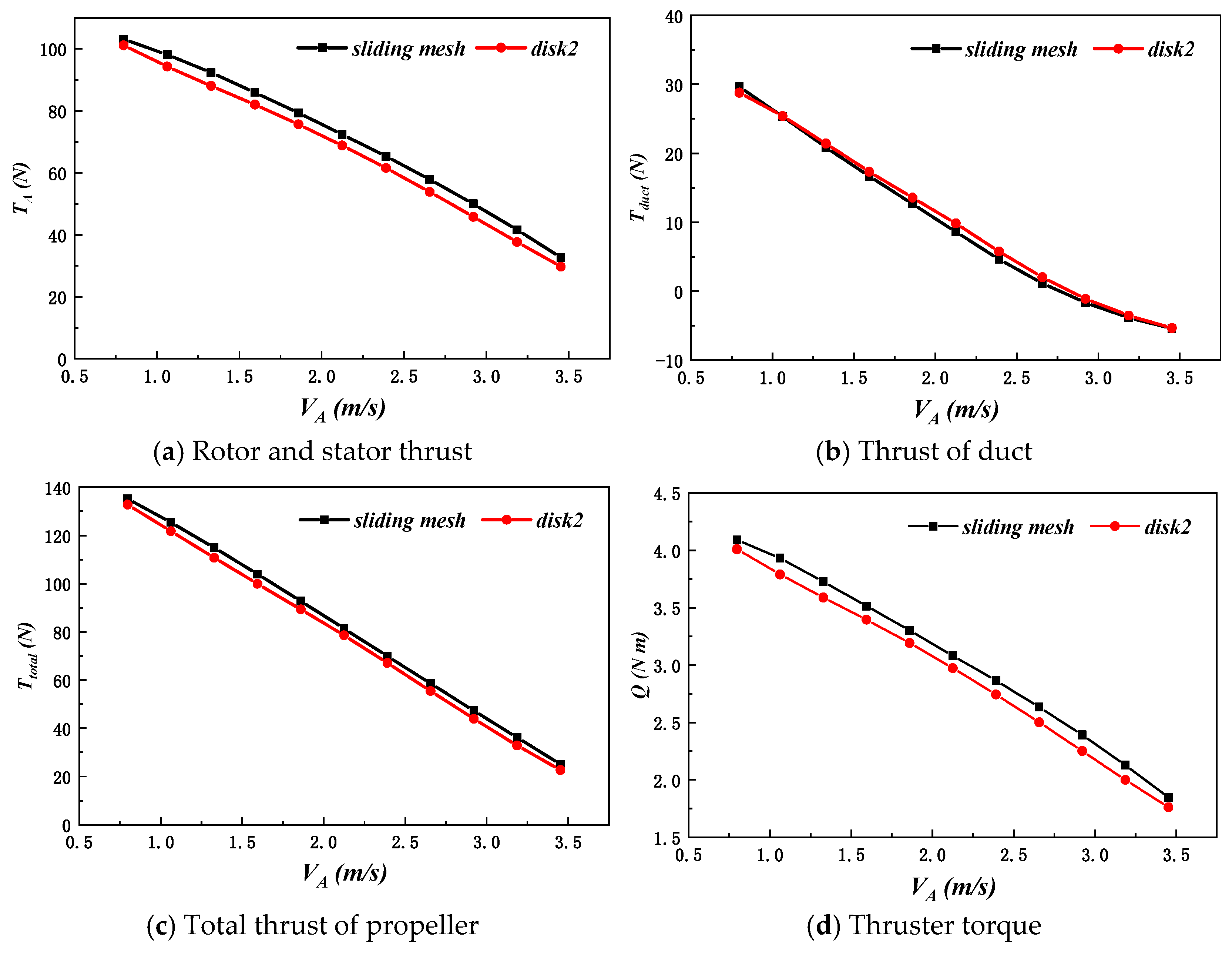
From Table 4, it can be observed that AD-R can accurately simulate the rotation of the rotor. The thrust coefficients calculated by both methods are within a 5% difference, and the error in the torque coefficient is less than 5%.

The forces of each component of propeller under the simulation of two methods are compared and analyzed. The comparison between the total thruster thrust calculated by AD-R and the sliding mesh method and the force on the conduit and other components is shown in Figure 10. Where $T_{duct}$ represents the force of the propeller duct, and $T_{total}$ represents the total thrust of the propeller.

As shown in Figure 10, AD-R can effectively simulate the forces on the entire propeller and its components. In most of the velocity range, the total thrust error between AD-R and the sliding mesh method is less than 5%. Additionally, the forces on the duct and rotor are in good agreement.

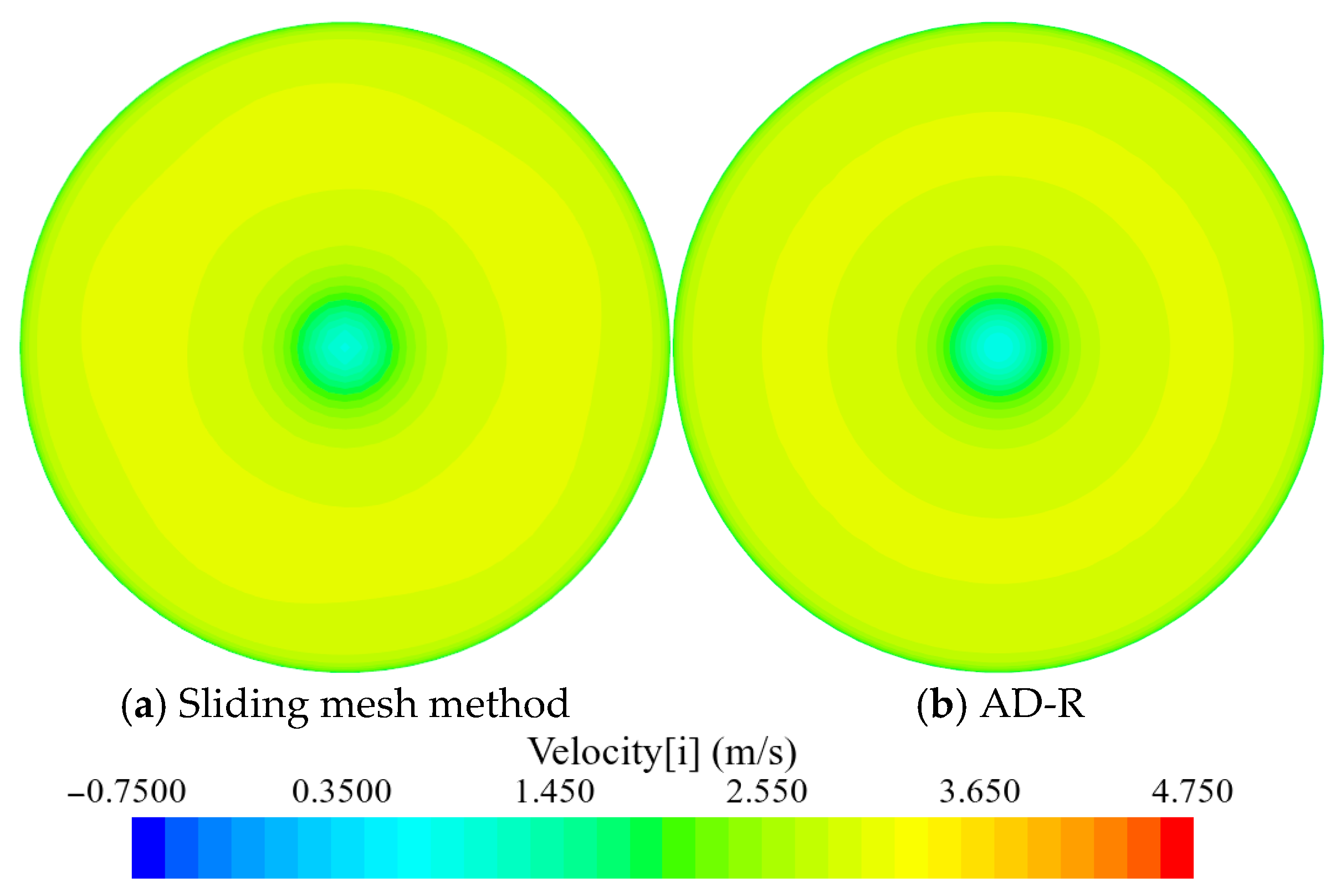
The flow field of AD-R during the simulation of propeller motion was also analyzed. A comparison of the flow field performance of the sliding mesh method and body force method was conducted at the same incoming flow velocity. When the flow velocity is 2.656 m/s, the comparison of the velocity distribution of the two methods at the same cross-section is shown in Figure 11 and Figure 12. As seen in the figures, the longitudinal velocity distribution at the inlet and outlet sections of the duct is nearly identical for both methods.

Additionally, the average axial velocity at both the inlet and outlet sections of the duct is calculated for different inflow velocities. The comparison between the two methods is shown in

Table 5. Comparison of the average axial velocity of the inlet and outlet sections of the duct.

${\mathit{V}}_{\mathit{A}}$ (m/s)	${\mathit{V}}_{\mathit{i}\mathit{n}\mathit{l}\mathit{e}\mathit{t}1}$ (m/s)	${\mathit{V}}_{\mathit{i}\mathit{n}\mathit{l}\mathit{e}\mathit{t}0}$ (m/s)	δ (%)	${\mathit{V}}_{\mathit{o}\mathit{u}\mathit{t}\mathit{l}\mathit{e}\mathit{t}1}$ (m/s)	${\mathit{V}}_{\mathit{o}\mathit{u}\mathit{t}\mathit{l}\mathit{e}\mathit{t}0}$ (m/s)	δ (%)
1.062	2.553	2.619	−2.50	2.881	2.951	−2.39
1.328	2.603	2.651	−1.83	2.939	2.989	−1.70
1.594	2.646	2.692	−1.71	2.989	3.036	−1.57
1.859	2.705	2.736	−1.14	3.059	3.089	−0.98
2.125	2.764	2.784	−0.70	3.130	3.147	−0.56
2.390	2.825	2.841	−0.57	3.197	3.211	−0.44
2.656	2.892	2.908	−0.55	3.269	3.282	−0.42
2.922	2.970	2.984	−0.50	3.350	3.363	−0.38
3.187	3.061	3.071	−0.31	3.446	3.452	−0.18
3.453	3.170	3.165	0.17	3.561	3.550	0.33

. Here, $V_{inlet}\text{\_}$ AD-R and $V_{outlet}\text{\_}$ AD-R represent the average axial velocities of the inlet and outlet sections of the duct, respectively, using the AD-R method. Meanwhile, $V_{inlet}$ and $V_{outlet}$ represent the average axial velocities at the inlet and outlet sections of the duct calculated using the sliding mesh method.

Under open-water conditions, the inflow at the duct inlet of the propeller is significantly influenced by the duct. Since AD-R retains the geometric shape of the propeller duct, as seen in Figure 11. And Table 5, the velocity distributions at the duct inlet cross-section obtained by both methods remain highly consistent. Furthermore, across different inflow velocities, the maximum error in the average axial velocity at the duct inlet cross-section computed by AD-R, compared to that obtained by the sliding mesh method, is only −2.50%.

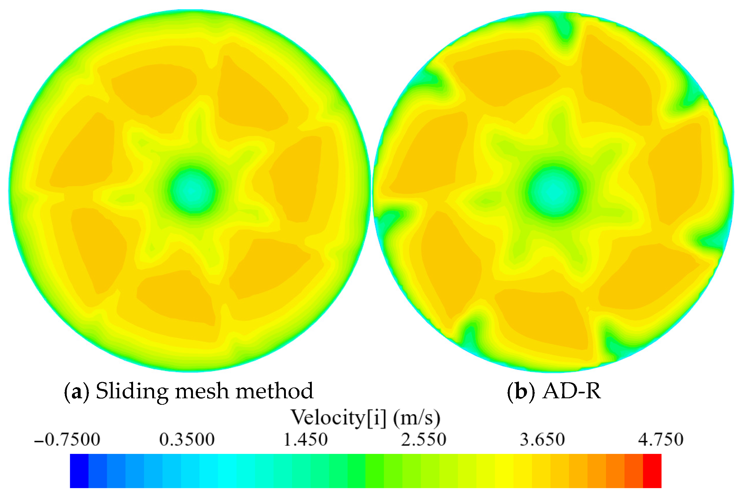
Different from the flow at the inlet of the duct, the outlet section of the duct is located at the end of the propeller, and the water flow at the outlet will be affected by the suction effect caused by the rotation of the rotor. At the same time, the existence of the rear stator will have a rectification effect on the fluid flowing through the rotating rotor, making the propeller outflow uniform. As shown in Figure 12 and Table 5, due to the rectification effect of the rear stator, the velocity distribution of the duct outlet section under the two methods is basically the same. Furthermore, under different inflow velocities, the maximum error between the average axial velocity of the duct outlet section calculated by AD-R and the sliding mesh method is only −2.39%, and the error gradually decreases with the increase of the inflow velocity.

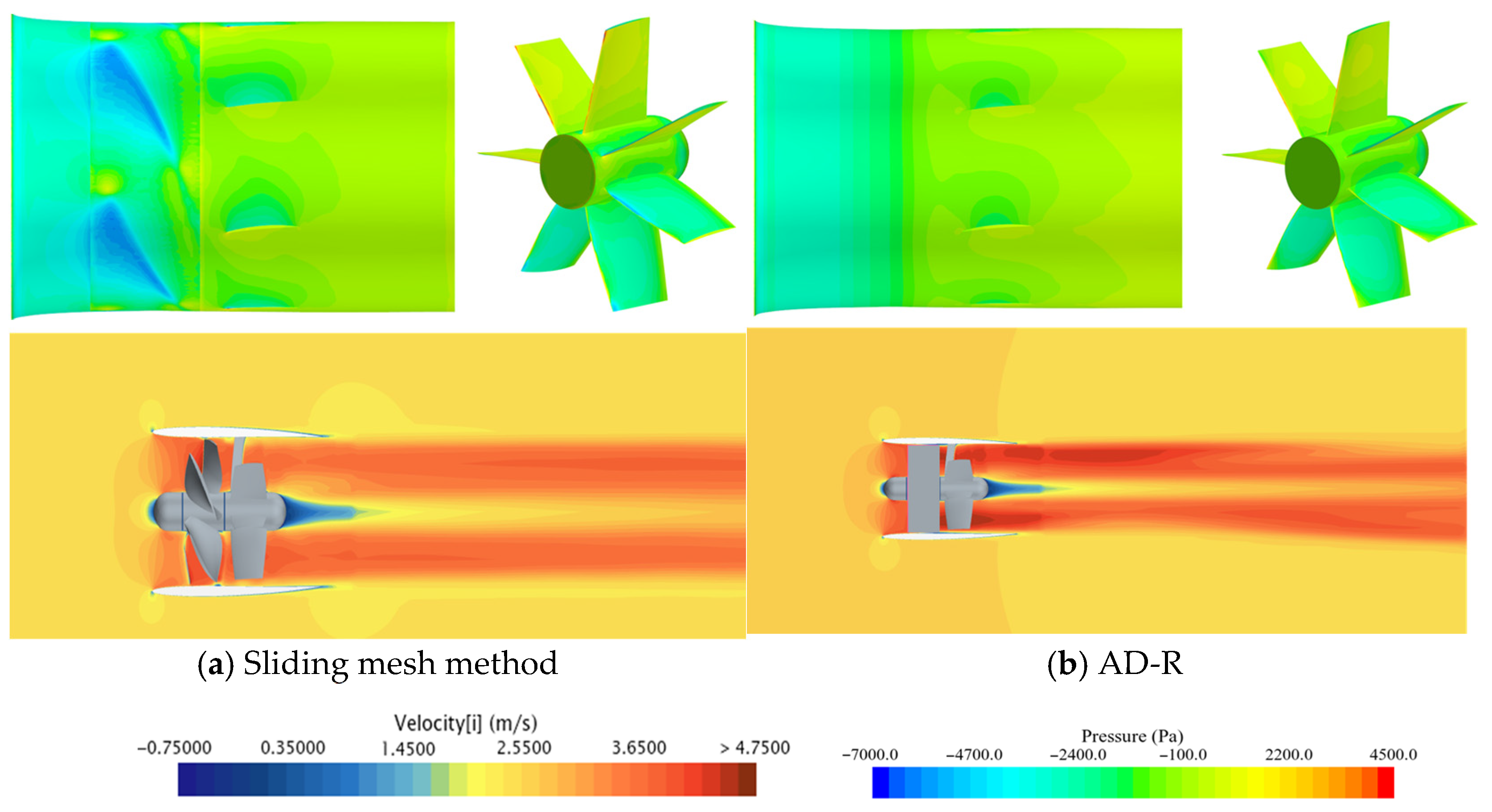
Figure 13 shows the comparison of the longitudinal velocity distribution on the XY plane, as well as the pressure distribution on the inner tube and stator surface, calculated by both methods.

As shown in Figure 13, when the incoming flow velocity is 2.656 m/s, and the velocity fields calculated by both methods are nearly identical, indicating that AD-R can effectively simulate both the internal and external flow fields of the propeller. However, noticeable differences are present in the pressure distributions along the inner duct and stator surfaces between the two methods.

Firstly, the sliding mesh method accurately simulates the actual rotor rotation. The gap between the rotor and the duct inner wall, along with the flow field variations induced by the rotor’s motion, creates distinct low-pressure regions near the rotor-adjacent duct walls. Additionally, the non-uniform flow field distribution downstream of the rotating rotor leads to localized high-pressure zones at the stator’s leading edge.

In contrast, the AD-R method substitutes the rotor geometry with an equivalent disk of the same diameter. This approach fundamentally differs from the unsteady flow characteristics created by physical blade rotation. As a result, AD-R yields a more uniform pressure distribution along the virtual disk-adjacent duct walls and lower absolute pressures on the stator blades.

5.2. Body Force Method Replaces Rotor and Stator Geometry

To assess the applicability of the modified body force method for replacing both the rotor and stator blades, the body force model (designated as AD-RS) is used to replace the rotor and stator blades, while retaining the shafting and duct. The schematic configuration of AD-RS is shown in Figure 14.

The rotational speed of the fixed body force is set to 16 rps, with a flow velocity range from 0.7968 to 3.4528 m/s. A comparison of the thrust coefficient and torque coefficient calculated by AD-RS and the sliding mesh method is provided in

Table 6. Comparison of propeller performance between the sliding mesh method and AD-RS.

${\mathit{V}}_{\mathit{A}}$ (m/s)	${\mathit{K}}_{\mathit{T}\mathit{A}2}$	${\mathit{K}}_{\mathit{T}\mathit{A}0}$	δ (%)	$10{\mathit{K}}_{\mathit{Q}2}$	$10{\mathit{K}}_{\mathit{Q}0}$	δ (%)
1.062	0.5819	0.5646	−3.90	1.4734	1.5283	−3.59
1.328	0.5432	0.5280	−4.65	1.3950	1.4489	−3.72
1.594	0.5062	0.4903	−4.59	1.3201	1.3661	−3.37
1.859	0.4669	0.4530	−4.63	1.2410	1.2839	−3.34
2.125	0.4246	0.4146	−4.89	1.1560	1.1983	−3.53
2.390	0.3798	0.3760	−5.83	1.0664	1.1137	−4.25
2.656	0.3324	0.3352	−6.92	0.9725	1.0239	−5.02
2.922	0.2829	0.2922	−8.30	0.8750	0.9296	−5.87
3.187	0.2326	0.2465	−9.42	0.7774	0.8276	−6.06
3.453	0.1836	0.1981	−9.18	0.6844	0.7178	−4.65

. The numerical simulation results of the sliding mesh method are represented by subscript0; the numerical simulation results of AD-RS are represented by subscript2.

As shown in Table 6, the thrust and torque coefficients of AD-RS are generally consistent with those of the sliding mesh method at lower flow velocities. However, as the flow velocity increases, the error between the two methods gradually increases.

To explore the reason of the large error in AD-RS at medium and high incoming flow velocities, the force and flow field characteristics of each propeller component simulated by both methods are compared. The comparison of the total thrust of the propeller and the forces on components such as the duct during the simulation calculations of AD-RS and the sliding mesh method is shown in Figure 15.

Based on the results in Table 6 and Figure 15, it is evident that the large error in the total thrust of the propeller is due to the significant discrepancies in the thrust and torque output of AD-RS at medium and high flow speeds. At an incoming flow velocity of 3.4528 m/s, the total thrust error of the propeller reaches −9.73%.

The comparison of the XY plane longitudinal velocity cloud diagram, pressure distribution on the inner tube surface, and velocity distribution at the outlet section of the duct calculated by AD-RS and the sliding mesh method is shown in Figure 16.

Both the rotor and stator blades are replaced geometrically in AD-RS, treating the rotor and stator as equivalent rotating components. Yet, this simulation cannot accurately replicate the effect of the rotor and stator on the flow field. As shown in Figure 16, since AD-RS replaces the stator’s actual geometric blades in the simulation, the stator’s rectifying action is entirely neglected. Consequently, the calculated flow field distribution at the conduit outlet does not match the actual flow field distribution at the thruster outlet, leading to an inaccurate simulation of the flow field inside the thruster. Furthermore, as the body force area in the AD-RS simulation is modeled as a cylinder and lacks the real rotor and stator blade geometries, the pressure distribution on the inner tube wall tends to be uniform across the entire section.

In conclusion, compared with AD-R, AD-RS treats the rotor and stator geometries as a unified rotating component, disregarding the stator’s rectifying role in the propeller. This approach results in an inability to accurately simulate the forces on each component of the propeller, the true distribution of the flow field within the propeller, and the flow behavior at the propeller’s outlet.

5.3. Influence of Different Inflow Velocity Planes on Body Force Method

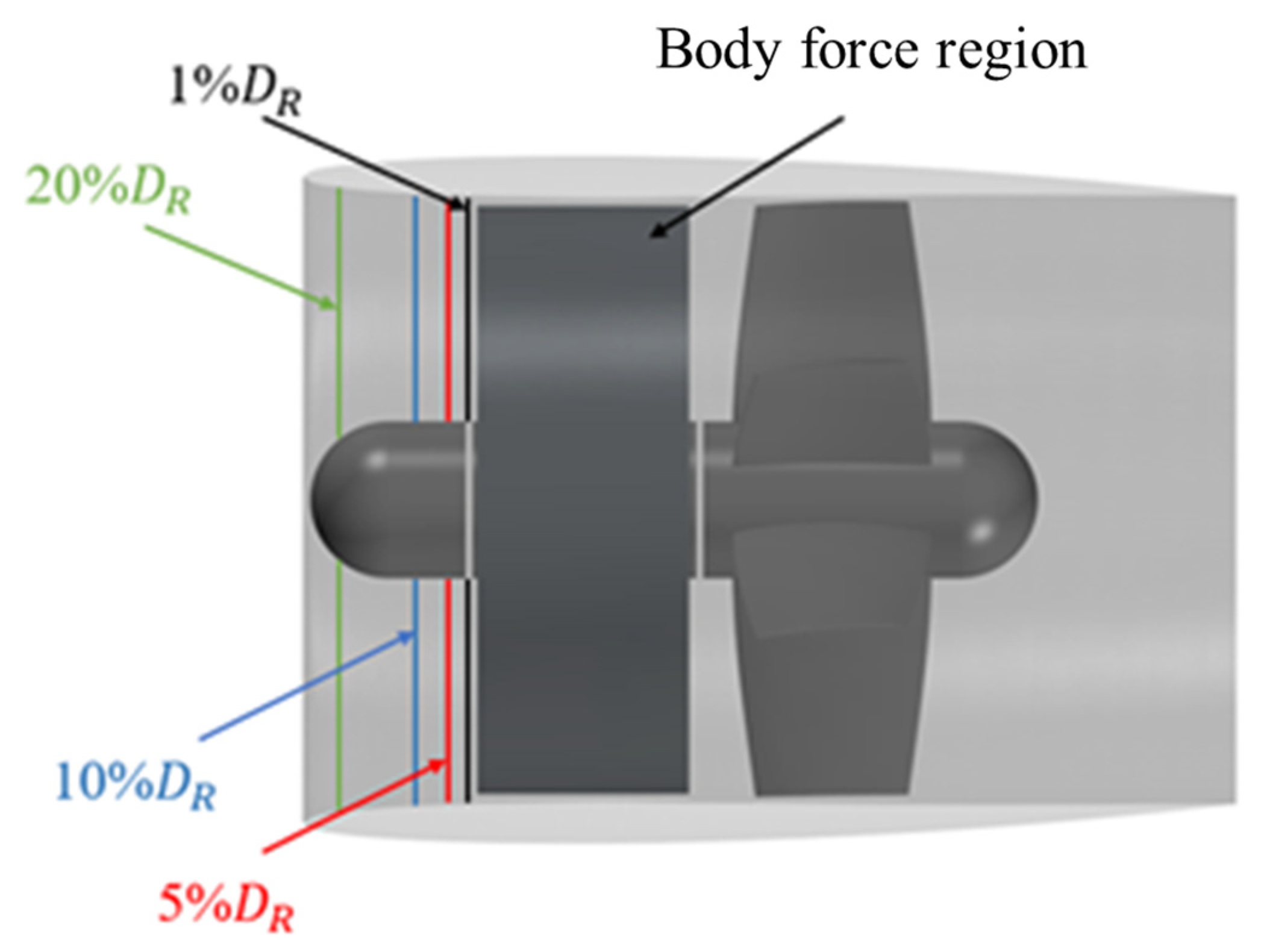
Based on the analysis of the body force method replacing the rotor, the position of the inflow velocity plane is adjusted to study the influence of inflow velocity plane placement on the results of the body force method. As shown in Figure 17, the improved body force method is used to simulate inflow velocity planes at four different positions. Each disk surface is offset by 1%$D_R$, 5%$D_R$, 10%$D_R$ and 20%$D_R$ relative to the propeller disk surface. The radius of each inflow velocity plane is the radius of the inner duct at the longitudinal position of the plane.

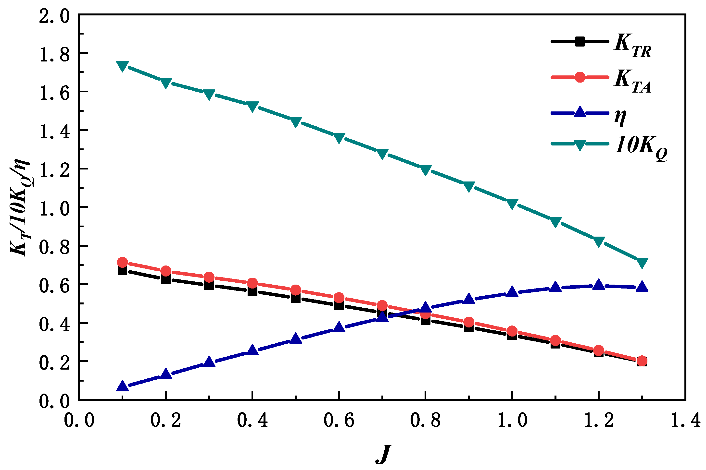
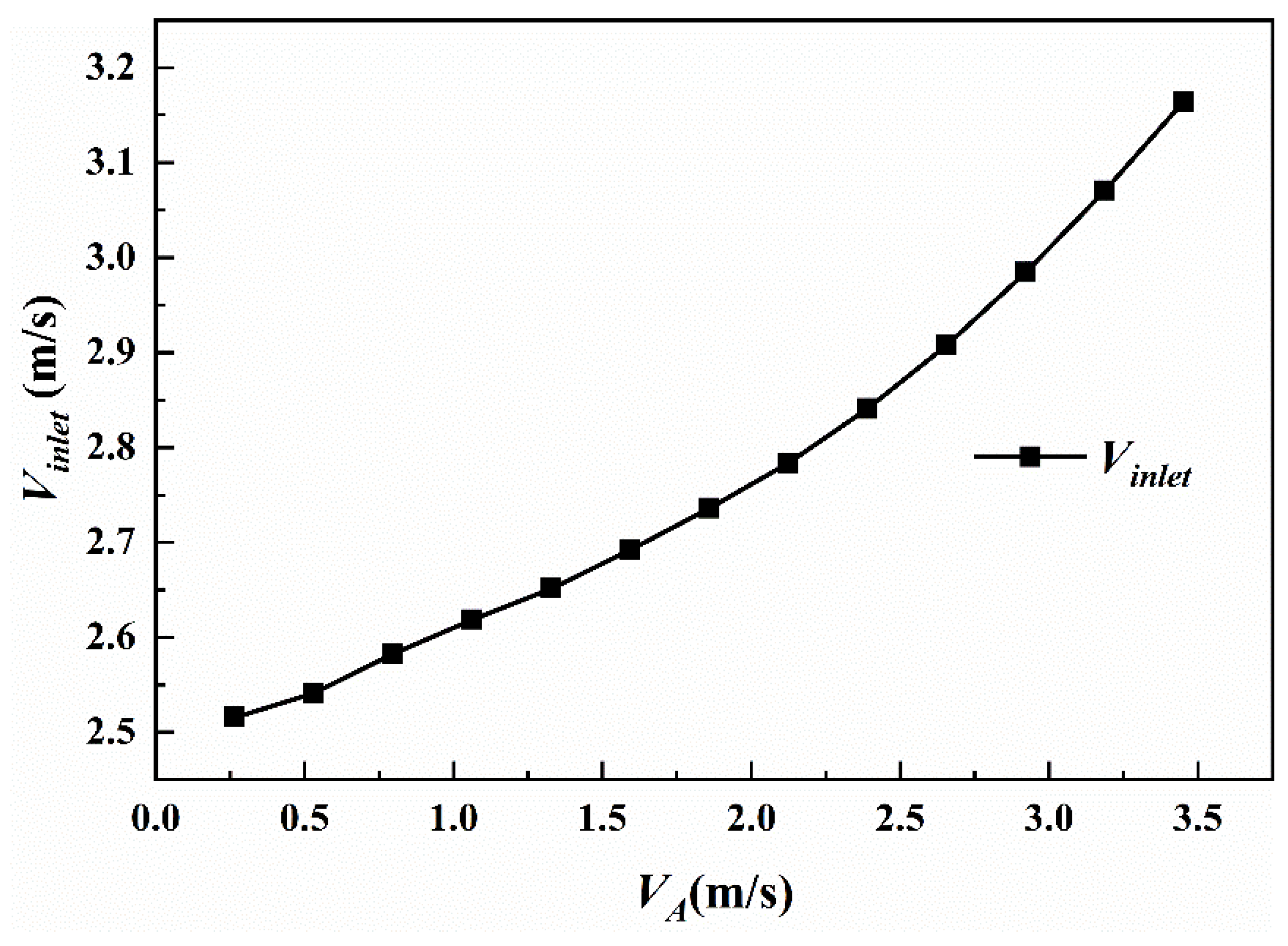
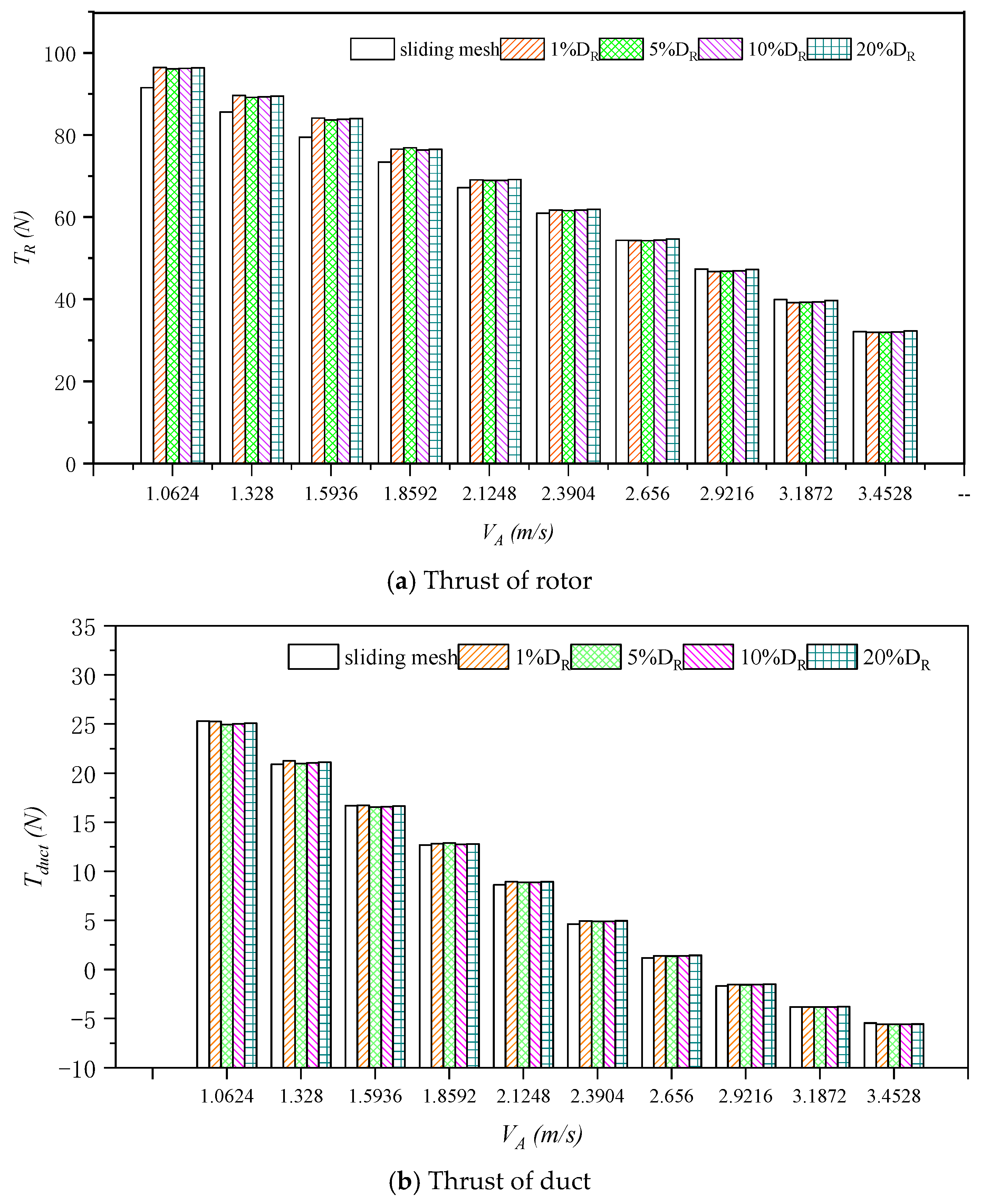
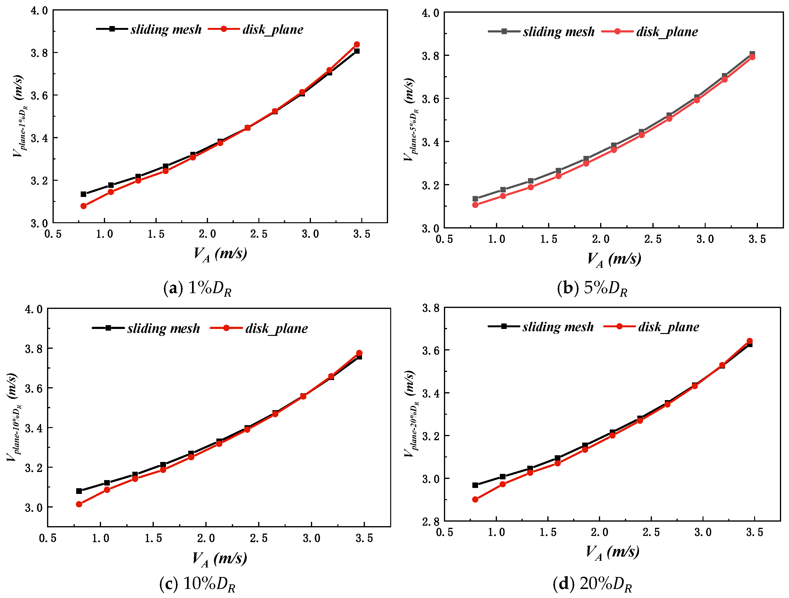
The flow velocity $V_A$ is modified using the average velocity $V_{plane}$ at the inflow velocity plane, which further adjusts the open water curve. Figure 18 shows the section-averaged velocity $V_{plane}$ distributions across the disk surfaces at different inflow velocities. As the offset increases from 1%$D_R$ to 20%$D_R$, the average cross-sectional velocity of the disk surface gradually decreases. This is due to the rotation and suction effect of the rotor, which accelerates the near flow field. Therefore, the closer the disk is to the propeller, the higher the average velocity at that disk.

Consistent with Section 5.1, the body force method is used to replace the rotor blades, and the shafting, stator blades and ducts are retained. The rotational speed of the fixed body force is 16 rps, and the velocity range is from 1.062 m/s to 3.453 m/s by changing the different incoming flow velocity $V_A$.

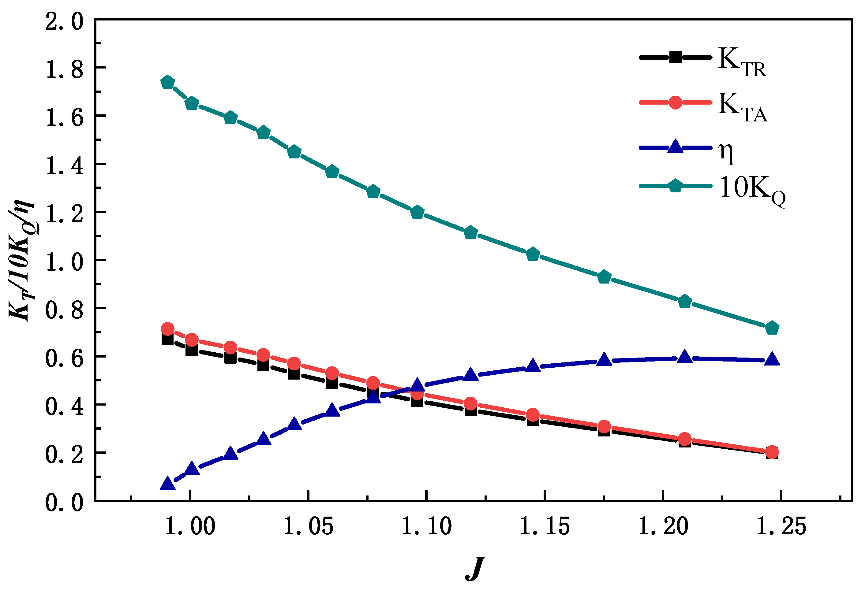
The open water characteristic curves corresponding to the four inflow velocity planes are input into the body force model to analyze the influence of the inflow velocity plane position on the results of the body force method. The hydrodynamic performance of the propeller is calculated for inflow velocity plane positions of 1%$D_R$, 5%$D_R$, 10%$D_R$ and 20%$D_R,$ respectively. The comparison of the thrust coefficient and torque coefficient of the propeller, as calculated by the body force method and the sliding mesh method, is shown in

Table 7. Comparison of thrust coefficient and torque coefficient between two methods.

(a) Thrust Coefficient
${\mathit{V}}_{\mathit{A}}$ (m/s)	${\mathit{K}}_{\mathit{T}\mathit{R}0}$	${\mathit{K}}_{\mathit{T}}\text{\_}\mathbf{1}\mathbf{\%}{\mathit{D}}_{\mathit{R}}$	${\mathit{K}}_{\mathit{T}}\mathbf{\text{\_}}\mathbf{5}\mathbf{\%}{\mathit{D}}_{\mathit{R}}$	${\mathit{K}}_{\mathit{T}}\mathbf{\text{\_}}\mathbf{10}\mathbf{\%}{\mathit{D}}_{\mathit{R}}$	${\mathit{K}}_{\mathit{T}}\mathbf{\text{\_}}\mathbf{20}\mathbf{\%}{\mathit{D}}_{\mathit{R}}$
1.062	0.5646	0.5889	0.5862	0.5877	0.5885
1.328	0.5280	0.5466	0.5458	0.5448	0.5476
1.594	0.4903	0.5066	0.5063	0.5048	0.5071
1.859	0.4530	0.4660	0.4668	0.4648	0.4683
2.125	0.4146	0.4259	0.4204	0.4254	0.4266
2.390	0.3760	0.3807	0.3800	0.3808	0.3822
2.656	0.3352	0.3351	0.3349	0.3357	0.3373
2.922	0.2922	0.2887	0.2889	0.2895	0.2913
3.187	0.2465	0.2420	0.2425	0.2429	0.2448
3.453	0.1981	0.1971	0.1971	0.1975	0.1995
(b) Torque Coefficient
${\mathit{V}}_{\mathit{A}}$ (m/s)	${\mathit{K}}_{\mathit{Q}\mathbf{0}}$	${\mathit{K}}_{\mathit{Q}}\mathbf{\text{\_}}\mathbf{1}\mathbf{\%}{\mathit{D}}_{\mathit{R}}$	${\mathit{K}}_{\mathit{Q}}\mathbf{\text{\_}}\mathbf{5}\mathbf{\%}{\mathit{D}}_{\mathit{R}}$	${\mathit{K}}_{\mathit{Q}}\mathbf{\text{\_}}\mathbf{10}\mathbf{\%}{\mathit{D}}_{\mathit{R}}$	${\mathit{K}}_{\mathit{Q}}\mathbf{\text{\_}}\mathbf{20}\mathbf{\%}{\mathit{D}}_{\mathit{R}}$
1.0624	0.1528	0.1585	0.1582	0.1583	0.1586
1.3280	0.1449	0.1496	0.1492	0.1493	0.1496
1.5936	0.1366	0.1424	0.1420	0.1421	0.1424
1.8592	0.1284	0.1324	0.1330	0.1322	0.1326
2.1248	0.1198	0.1225	0.1225	0.1224	0.1228
2.3904	0.1114	0.1127	0.1126	0.1127	0.1131
2.6560	0.1024	0.1027	0.1027	0.1028	0.1033
2.9216	0.0930	0.0923	0.0925	0.0925	0.0930
3.1872	0.0828	0.0816	0.0819	0.0819	0.0825
3.4528	0.0718	0.0710	0.0712	0.0712	0.0718

.

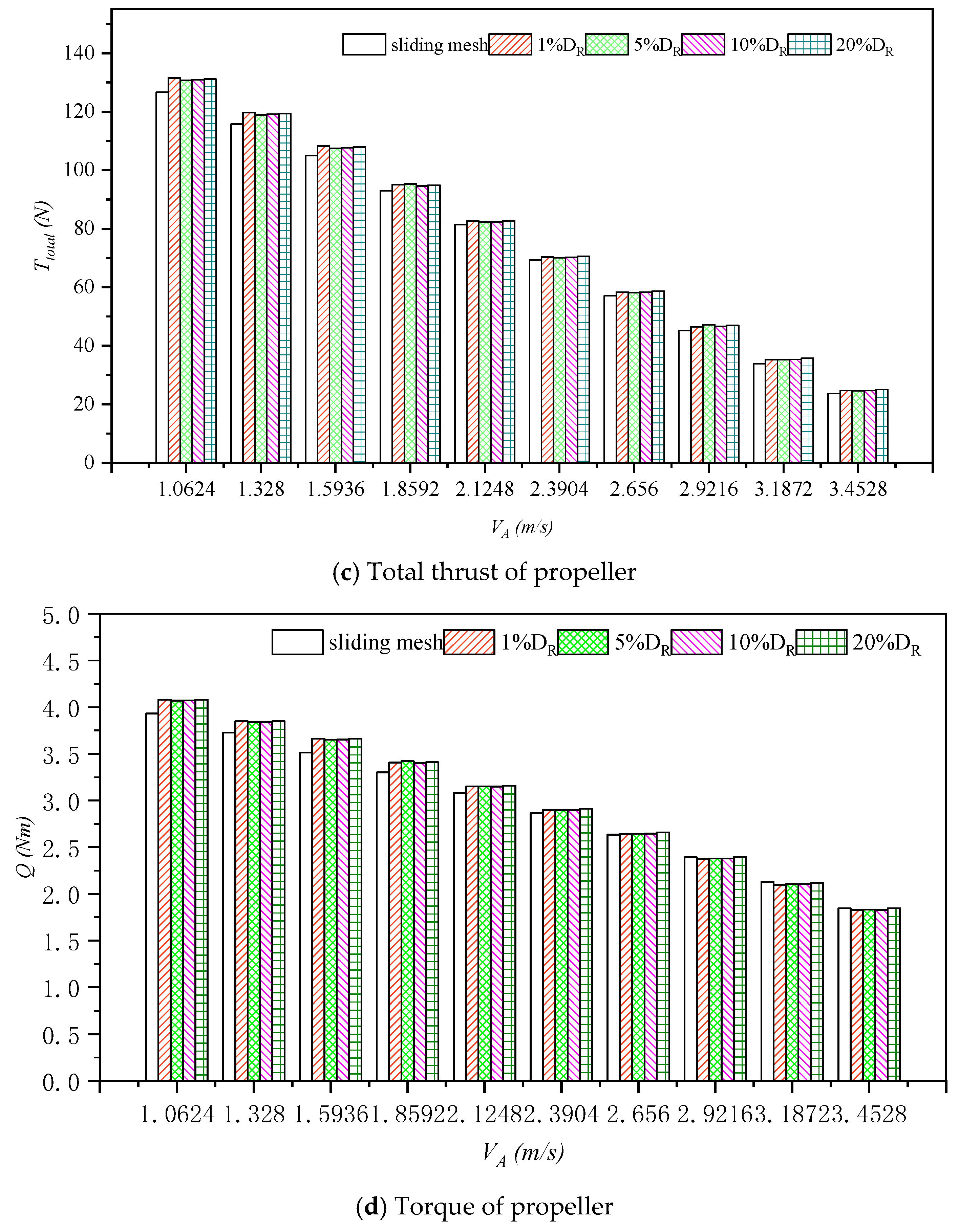
It can be seen from Table 7 that in the numerical simulation, when the body force method employs different inflow velocity planes, the calculated thrust coefficient and torque coefficient are consistent with changes in the inflow velocity, Moreover, the error compared to the sliding mesh method remains consistently minor across all cases.

In order to analyze the accuracy of the body force method to simulate the open-water performance of the propeller when the inflow velocity plane at different positions is calculated, the force of each component of the propeller is compared and analyzed when the inflow velocity plane at different positions is calculated. The force on each component of the propeller is shown in Figure 19. It can be seen from the results in Figure 19 that when the inflow velocity planes at different positions are taken in the body force method, the force results of each component obtained by numerical simulation are not much different, and are in good agreement with the calculation results of the sliding mesh method.

Additionally, to analyze the flow field characteristics when the body force method is applied at different inflow velocity planes for propeller motion simulation, the flow field performance of the body force method after calculation stability is compared and analyzed at the same inflow velocity.

At different inflow velocities, the average axial velocity at each inflow velocity plane, calculated by the two methods, is shown in Figure 20. Here, $V_{plane-1\%D_R}$, $V_{plane-5\%D_R}$, $V_{plane-10\%D_R}$ and $V_{plane-20\%D_R}$ denote the average axial velocity at the inflow velocity plane with offsets of 1%, 5%, 10%, and 20%, respectively. The velocities calculated by body force method are in good agreement with those calculated by the sliding mesh method. The maximum errors are as follows: −1.77% for $V_{plane-1\%D_R}$, −2.2% for $V_{plane-5\%D_R}$, 2.16% for $V_{plane-10\%D_R}$, and 3.28% for $V_{plane-20\%D_R}$.

In addition, the average axial velocity of the duct outlet section of the propeller calculated by different inflow velocity planes is compared, as shown in

Table 8. Average axial velocity of duct outlet section.

${\mathit{V}}_{\mathit{A}}$ (m/s)	${\mathit{V}}_{\mathit{o}\mathit{u}\mathit{t}\mathit{l}\mathit{e}\mathit{t}0}$ (m/s)	${\mathit{V}}_{\mathit{o}\mathit{t}-1\mathbf{\%}{\mathit{D}}_{\mathit{R}}}$ (m/s)	${\mathit{V}}_{\mathit{o}\mathit{t}-5\mathbf{\%}{\mathit{D}}_{\mathit{R}}}$ (m/s)	${\mathit{V}}_{\mathit{o}\mathit{t}-10\mathbf{\%}{\mathit{D}}_{\mathit{R}}}$ (m/s)	${\mathit{V}}_{\mathit{o}\mathit{t}-20\mathbf{\%}{\mathit{D}}_{\mathit{R}}}$ (m/s)
1.062	2.951	2.929	2.915	2.917	2.919
1.328	2.989	2.978	2.968	2.970	2.972
1.594	3.036	3.019	3.011	3.013	3.015
1.859	3.089	3.079	3.081	3.075	3.077
2.125	3.147	3.142	3.139	3.139	3.142
2.390	3.211	3.209	3.205	3.207	3.210
2.656	3.283	3.282	3.280	3.281	3.285
2.922	3.363	3.366	3.364	3.366	3.369
3.187	3.452	3.462	3.461	3.462	3.466
3.453	3.550	3.574	3.572	3.573	3.577

. Here,$V_{ot-1\%D_R}$, $V_{ot-5\%D_R}$, $V_{ot-10\%D_R}$ and $V_{ot-20\%D_R}$ represent the average axial velocity of the duct outlet section with the inflow velocity plane offset of 1%$D_R$, 5%$D_R$, 10%$D_R$ and 20%$D_R$, respectively.

It can be seen from Table 8 that the error between the average axial velocity of the duct outlet section of the propeller and the calculation result of the sliding mesh method is small when the inflow velocity plane is different.

Figure 21 shows the comparison of the longitudinal velocity distribution of the XY plane, the pressure distribution of the inner duct, and the velocity distribution of the outlet section of the duct calculated by body force method under different inflow velocity planes. The results indicate that the inflow velocity plane position has little effect on the flow field of the propeller.

In summary, when varying the positions of the inflow velocity plane, there is minimal impact on the calculation results of the improved body force method. Therefore, when simulating the propeller in open water, any plane between the duct inlet and the propeller disk surface can be chosen as the inflow velocity plane for the improved body force method. The average cross-sectional velocity at this plane can be used to correct the open water curve. This approach ensures the accuracy of the force on each component of the propeller when using the body force method for numerical simulations, and the flow field remains consistent with that calculated by the sliding mesh method.

6. Conclusions

This paper investigates the construction of the body force model for a submerged waterjet. A series of numerical simulations using the RANS method were conducted, and the numerical results showed good agreement with experimental data, verifying the reliability of the numerical method. A body force model suitable for submerged waterjet propulsion systems was developed, and the results were compared with those of the sliding mesh method under uniform inflow conditions. Additionally, the influence of the inflow velocity plane position on the results of the body force model was analyzed. The main conclusions are as follows:

(a)

A body force model (AD-R) was developed to independently characterize rotor and stator forces. Under uniform inflow conditions, AD-R predicted rotor thrust and torque within 5% error compared to the sliding mesh method, with force distributions on propeller components and flow fields showing essential agreement.

(b)

Compared with AD-R, AD-RS treats both rotor and stator geometries as a single rotating component, neglecting the stator’s rectifying effect. Consequently, while yielding acceptable accuracy at low inflow speeds, this model exhibits significantly increasing errors with rising flow velocity. It is therefore unsuitable for simulating submerged waterjet propulsion systems.

(c)

The influence of inflow velocity plane position on model accuracy was analyzed. Results demonstrate that the AD-R model maintains consistent performance across varying inflow plane locations, confirming its robustness for engineering simulations.

This study primarily focused on uniform inflow conditions, and future research can address the following areas: (1) optimizing the body force model to handle complex conditions such as non-uniform inflow and turbulence, and evaluating its applicability, and (2) studying the multi-field coupling effects between the propeller, hull, and other systems, and analyzing their influence on hydrodynamic performance. Such efforts would promote the broader application of the body force model in engineering practice and provide theoretical support for the design and optimization of submerged waterjet propellers.