Energy-Efficient Scheduling for Resilient Container-Supply Hybrid Flow Shops Under Transportation Constraints and Stochastic Arrivals

Abstract

Although dynamic, energy-efficient container-supply hybrid flow shops have attracted increasing attention, most existing research overlooks how transportation within container production affects makespan, resilience, and sustainability. To bridge this gap, we frame a resilient, energy-efficient container-supply hybrid flow shop (TDEHFSP) scheduling model that utilizes vehicle transportation to maximize operational efficiency. To address the TDEHFSP model, the study proposes a Q-learning-based multi-swarm collaborative optimization algorithm (Q-MGCOA). The algorithm integrates a time gap left-shift scheduling strategy with a machine on–off control mechanism to construct an energy-saving optimization framework. Additionally, a predictive–reactive dynamic rescheduling model is introduced to address unexpected task disturbances. To validate the algorithm’s effectiveness, 36 benchmark test cases with varying scales are designed for horizontal comparison. Results show that the proposed Q-MGCOA outperforms benchmarks on convergence, diversity, and supply-chain resilience while lowering energy utilization. Moreover, it achieves about an 8% reduction in energy consumption compared to traditional algorithms. These findings reveal actionable insights for next-generation intelligent, low-carbon container production.

1. Introduction

The Hybrid Flow Shop Problem (HFSP) refers to a production workshop where multiple processes are arranged in a flow line, with at least one process involving multiple machines. The primary challenge is organizing the job sequencing and machine scheduling. HFSP involves multiple processing stages and is known for its flexibility. It is particularly suited for scheduling small batch, multi-variety production tasks, making it widely applicable in manufacturing. To tackle environment conservation and emission reduction concerns, the energy-optimization process of HFSP will be an important research focus.

For energy-efficient hybrid flow shop scheduling (EHFSP), most studies aim to optimize both the makespan ${ (C}_{max})$ and the total energy consumption (TEC). Most studies on energy-efficient hybrid flow shop scheduling (EHFSP) focus on a single energy-efficient strategy, such as speed-scaling, turn-on/off mechanisms, or time-of-use pricing.

The speed-scaling strategy refers to the dynamic adjustment of processing speeds during processing. Wang et al. [1] used the speed-scaling strategy for machines and an extended non-dominated sorting genetic algorithm (NSGA-II) to reduce $TEC$ without affecting work efficiency. Wang et al. [2] provided an energy-efficient strategy on account of speed selection that optimizes both $TEC$ and $C_{max}$, taking into account the characteristics of EHFSP. Goli et al. [3] introduced a new meta-heuristic algorithm for determining batch size and speed per machine to minimize $TEC$ and $C_{max}$ simultaneously.

Time-of-use pricing mechanisms aim to reduce $TEC$ and carbon emission costs by optimizing electricity usage time. Geng et al. [4] researched the distributed heterogeneous re-entrant HFSP issue with the following dependent times under time-of-use pricing constraints and issued a multi-objective artificial bee colony algorithm to deal with the challenge. Ho et al. [5] proposed an exact method based on logical Benders decomposition to tackle the two-machine issue with time-of-use pricing to minimize TEC. Complementing energy-saving efforts inside container terminals, the ship side is also moving toward alternative fuels to comply with the forthcoming Maritime ETS. Sun et al. [6] analyze shipping alliances and show that deploying LNG-powered vessels can cut ETS allowance costs by roughly 12–18% while enhancing inter-alliance competitiveness. Their work reinforces the need to couple vessel-fuel decisions with landside scheduling models targeting CO₂/TEU reduction, thereby justifying the sustainability objective adopted in this study.

In contrast to the speed-scaling strategy, there has not been that much attention paid to the turn-on/off mechanism. Mu et al. [7] considered the turn-on/off mechanism, established a model for the collaborative scheduling of heterogeneous multi-stage HFSP, and proposed a method combining the moth firefly optimization algorithm (NSGA-II-MFO). The study puts forward an energy-efficient strategy derived from the “left shift” of time intervals to minimize TEC, considering the previously discussed turn-on/off strategy.

The HFSP machining process affects the manufacturing plant’s productivity and the production plan’s implementation, so some scholars have studied the dynamic shop scheduling DHFSP. The most common dynamics are the emergence of recent work demands and equipment failure. Tao et al. [8] developed the NSGA-II with Q-learning to solve the disruption of the arrival of new work. Wang et al. [2] developed research on the DEHFSP scheduling issue of machine failures and proposed an improved multi-objective firefly algorithm that guarantees to reduce $TEC$ without affecting productivity. Jiang et al. [9] put forward a multi-faceted immune system-inspired algorithm combining a Q-learning algorithm to optimize $TEC$, $C_{max}$ and average agreement index with three objectives by simultaneously considering the effects of the above two dynamics.

Dynamic scheduling can be categorized as fully responsive planning, anticipation-based adaptable planning, and resilient forward-looking planning.

Fully responsive scheduling deals with changing circumstances by continuously observing the state of the job shop and does not require a predefined scheduling scheme. Luo et al. [10] introduced a ubiquitous manufacturing environment with immediate data feedback channels, information exchange, and alignment mechanisms, and a multi-cycle hierarchical scheduling system to solve the HFSP scheduling issue with continuous new jobs. Ghaleb et al. [11] proposed an active–passive spontaneous scheduling model to deal with uncertain, unknown workloads and machine breakdown.

Robust, proactive scheduling refers to generating predetermined scheduling plans based on a pre-training process to ameliorate system instability caused by frequent rescheduling. Ashraf et al. [12] study the importance of leveraging technology and distance learning solutions to ensure continuity in education, emphasizing the need for innovative and sustainable approaches to teaching and learning in crisis situations. ElMekkawy et al. [13] exploited the machine’s flexibility and predicted equipment malfunctions, creating an anticipatory scheduling way to tackle the real-time scheduling challenges of a versatile job shop with potential machinery failures.

Unlike robust proactive scheduling, predictive–reactive scheduling adopts a pre-scheduling scheme in a static environment. Then, it modifies the pre-scheduling scheme to acquire a new scheduling arrangement according to the latest situation after a scenario emerges or at a fixed period. There are also three predictive–reactive scheduling methods: partial scheduling, complete rescheduling, and insertion rescheduling. Predictive–reactive scheduling approaches primarily include partial schedule adjustment, full rescheduling, and task insertion. Duan et al. [14] analyzed manufacturing system robustness under disruptions while balancing ${ C}_{max}$, $TEC$, and resource reusability. A dynamic HFSP framework was introduced by Luo et al. [15], combining complete rescheduling strategies with a hybrid parallel genetic algorithm to manage new job arrivals. Ghaleb et al. [16] designed a genetic algorithm hybridizing predictive and reactive phases to optimize disruption recovery costs and tardiness penalties in complex scenarios. In this paper, the three predictive–responsive scheduling methods are applied simultaneously, and the most robust method is selected for rescheduling based on an instability measure.

With the increasing research on shop scheduling, some scholars began to explore the impact of the transportation process on shop scheduling problems. Li et al. [17] take the transportation time of AGVs into account and offer an innovative way to solve the synthesis, production, and transportation scheduling in the HFSP environment. Luo et al. [18] incorporated transport resource constraints into the Distributed Assembly Flow Shop Scheduling Problem (DAFSP), enhancing a decomposition-based multi-objective evolutionary algorithm (IMOEA/D) for $C_{max}$ optimization. Cai et al. [19] investigated the distributed assembly HFSP scheduling issue, which consists of manufacturing and transportation, and offered a shuffled frog learning algorithm (QSFLA) with Q-learning to minimize the completion time. While much of the research in flow shop scheduling focuses on distributed flow shops, there is comparatively less research on transportation energy consumption. Zhang et al. [20] issue a decomposition-based three-stage multi-objective approach (TMOA/D) to solve the EHFSP model by combining three scenarios: the energy used by machinery during standby and preparation periods and work during transportation for the first time.

The emergence of various incidents and the transportation of jobs within the shop scheduling are unavoidable in real production processes. However, no research has been conducted to address both situations in a multi-stage HFSP configuration. The study examines an energy-efficient hybrid flow shop scheduling issue (TDEHFSP) that accounts for the untimely introduction of new jobs and the transportation process between processing stages, with the objective of simultaneously minimizing $C_{max}$ and $TEC$.

For years, reinforcement learning techniques have gained a surge in interest in solving optimization problems. There are two main applications for shop scheduling. The first is to use reinforcement learning as an advanced hyper-heuristic to guide the finding of the set of low-level heuristics. Zhang et al. [21] suggested a Q-learning-based hyper-heuristic evolutionary algorithm (QLHHEA) to solve the DABFSP problem aiming at minimization. Zhang et al. [22] developed the Q-learning advanced strategy to find out the most appropriate low-level heuristic (LLH) from a pre-designed set based on the insights provided by the efficacy of the low-level heuristic. However, the hyper-heuristic algorithm is less suitable for dynamic scheduling research because it requires targeted design of LLHs and has high computational complexity.

The second one is reinforcement learning combined with meta-heuristic algorithms, which can enhance the search efficacy and performance of the algorithm. Jia et al. [23] developed a Q-learning-driven multi-swarm pattern mining algorithm (MPMA) to address distributed assembly HFSP with adaptive preventive maintenance. Li et al. [24] tackled energy-efficient HFSP by minimizing delays, energy costs, and carbon trading expenses through a dual Q-table reinforcement learning mechanism integrated with a generalized variable neighborhood search-enhanced NSGA-II. Zhang et al. [25] focused on the heterogeneous DEHFSP and simultaneously optimized ${ C}_{max}$ and $TEC$ by utilizing Q-learning to guide the variable neighborhood search. Additionally, they proposed a multi-objective modal factorization algorithm combining particle swarm optimization PSO and Q-learning local search to improve the exploration capability of PSO.

These studies demonstrate that the algorithm combining Q-learning and PSO to drive the meta-heuristic process is expected to enhance exploration capability. MGPSO is a multiple swarm particle swarm optimization algorithm proposed based on PSO. Q-learning in this study is employed to learn the optimal behavior on the part of the operators, ensuring the selection of a suitable local search operator throughout the iterative procedure.

The specific value of this paper is threefold. First, we propose a novel energy-efficient hybrid flow shop scheduling problem (TDEHFSP) that simultaneously accounts for dynamic job arrivals and transportation processes, addressing the gap in optimizing both transportation energy consumption and dynamic disturbances in multi-stage HFSP. Second, we develop a multi-objective MINLP model integrating a time interval left-shift strategy and machine turn-on/off mechanisms, providing a quantitative tool for low-carbon production. Third, the proposed Q-MGCOA algorithm dynamically selects search operators via Q-learning, significantly improving convergence and diversity. This research not only reduces makespan and energy consumption but also offers new insights for real-time scheduling and cost control in port container supply chains.

2. Materials and Methods

2.1. Mathematical Modeling

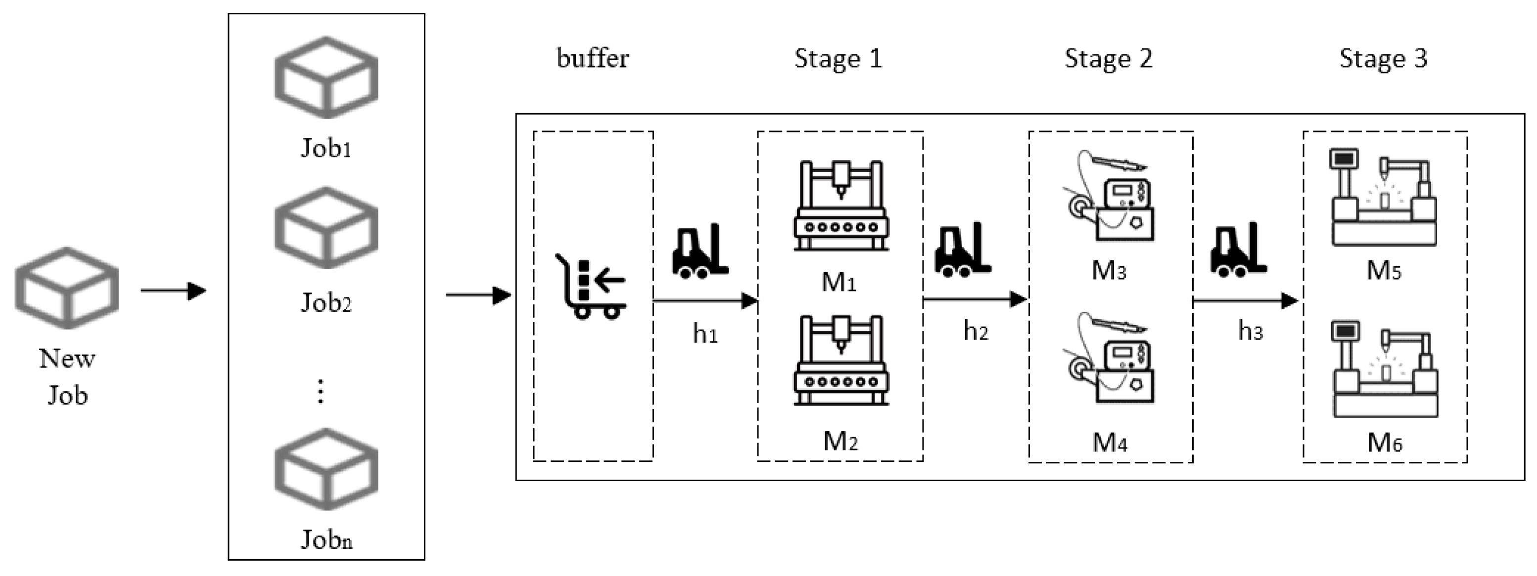
2.1.1. Problem Formulation

This paper studies a multi-stage TDEHFSP. A framework diagram of a hybrid flow shop dynamic scheduling optimization system considering the transportation process is shown in Figure 1. Each machining stage includes one or more machining machines with the same function but varying efficiency. There is a buffer zone before machining stage 1, and all the jobs are stored in the buffer zone at the beginning for use in later processes. Additionally, the study encompasses the transportation of jobs between the various stages of the process, with corresponding transport vehicles established between the stages.

The TDEHFSP framework involves processing a collection of jobs across sequential phases, where each phase utilizes m dedicated machines. Each job consists of an ordered chain of operations and exhibits dynamic arrival patterns, meaning new jobs may emerge unpredictably after initial scheduling execution. Inter-phase material transfer is managed by a specialized transport unit that operates in three distinct modes: no-loading, loading, and idle waiting. Notably, energy consumption characteristics differ between loaded and unloaded transit modes due to varying operational speeds and power requirements, while the standby mode maintains zero energy expenditure.

The assumptions are as follows:

• Each machine can process only one task at any given moment.
• Every job must be processed by exactly one designated machine per operation.
• Job processing must proceed continuously once initiated, without suspension or interruption.
• All resources (machines/transport units) remain fully operational and available throughout the production timeline.
• Each operation can be executed on any eligible machine from the available set.
• Machines operate in four distinct modes: active processing, standby, maintenance, and shutdown, each with unique energy consumption patterns.
• Transport speed varies between the loaded and unloaded states of the transfer unit.
• Initial locations of all jobs and transport units reside in an unbounded-capacity buffer zone.
• Transportation assignments are exclusive—each task requires dedicated transporter allocation, and each transporter handles only one task concurrently.
• Potential conflicts or collision avoidance between transporters are excluded from consideration.
• Transport distance computations employ Manhattan metric principles.
• Existing schedules remain reconfigurable for unprocessed operations when new jobs arrive.
• New job arrivals occur stochastically without predefined temporal patterns.

2.1.2. Modeling Building

In order to establish a multi-objective optimization framework for the TDEHFSP, which is suited for container-supply situations, targeting dual minimization of $C_{max},$ and $TEC$, a model by previous studies of Zhang et al. [26] has been referred to, which is established as follows, which the notations are given in

Table 1. Notations of present study.

Parameters	Definition	Parameters	Definition
$n$	Sum of jobs number.	$e$	The $e$-th transport task, ($e=1,\dots ,\mathrm{g}$)
$s$	Sum of stages number	$h_j$	Transport vehicle $\mathrm{i}\mathrm{n}\mathrm{d}\mathrm{e}\mathrm{x}$, ${(h}_j=1,\dots ,\mathrm{q})$
$m$	Sum of corresponding workshop machines	$v_{zn},v_{zl}$	No-load/load transport speed of transport vehicles
$j$	Stage index $(j=1,\dots ,s)$	$O_{ij}$	$j$-th operation of job $i$
$i$	Job index $(i=1,\dots ,n)$	$x_b$	Horizontal coordinate of the buffer
$N\_i$	New job index $(N\_i=1,\dots ,\mathrm{r})$	$(x_{k_j},y_{k_j})$	Coordinates of $k_j$
$k_j$	$\mathrm{M}\mathrm{a}\mathrm{c}\mathrm{h}\mathrm{i}\mathrm{n}\mathrm{e}\mathrm{i}\mathrm{n}\mathrm{d}\mathrm{e}\mathrm{x}(k_j=1,\dots ,m$)	$P_{k_j},{IP}_{k_j}$	Processing/standby power of $k_j$
$C_i$	Transportation time of the first job	$C_{is}$	Ending time of final stage jobs
$P_{Zn},P_{Zl}$	No-load/load transport power of transport vehicles	$P_{k_j}^{on}{,P}_{k_j}^{off}$	Turn-on/off power of $k_j$
$T_{k_j}^{on},T_{k_j}^{off}$	Turn-on/off time of $k_j$	$T_{k_j}$	Time constant
$T_{ij{i}^{\mathrm{*}}j}^{k_j}$	Idle time of $k_j$	$T_{N\_i}^{on}$	Time to start processing of new jobs
$t_{ij}^{k_j}$	Processing time of $O_{ij}$ on $k_j$	$T_{N\_i}^A$	Arrival time of new jobs
$NS{T}_{ij},NE{T}_{ij}$	Starting/ending time of the no-load transport task $O_{ij}$	$LS{T}_{ij},LE{T}_{ij}$	Starting/ending time of the load transport task $O_{ij}$
Variables
$a_{ij}^{k_j}$	1 if the operation $O_{ij}$ is dealt with on the machine $k_j$, 0 otherwise.
$b_{i^{\mathrm{*}}}^{k_j}$	1 if job $i^{\mathrm{*}}$ is the subsequent job of job $i$ dealt with by machine $k_j$, 0 otherwise.
$c_{i{k}_j}^{h_j}$	1 if job $i$ is dealt with on the machine $k_j$ and is transported by the transport vehicle $h_j$, 0 otherwise.
$d_{ie{i}^{\mathrm{*}}{e}^{\mathrm{*}}}^{h_{j^{\mathrm{*}}}}$	1 if operation ${ O}_{i^{\mathrm{*}}{j}^{\mathrm{*}}}$ is $O_{ij}$ is a post-operation dealt with on machine $k_j$, 0 otherwise.
$e_{i{k}_j}^{k_{j^{\mathrm{*}}}}$	1 if the subsequent operation of job $i$ after processing in machine $k_j$ is carried out in machine $k_{j^{\mathrm{*}}}$, 0 otherwise.

.

Minimize the defining equation:

$$min{C}_{max}=\mathrm{m}\mathrm{i}\mathrm{n}\left(C_i+\sum _{i=1}^n\mathrm{m}\mathrm{a}\mathrm{x}\left(C_{is}\right)\right)$$

(1)

$$minTEC=\min \left(E_1+E_2+E_3+E_4+E_5\right)$$

(2)

$$E_1=\sum _{k_j=1}^m\sum _{i=1}^n\sum _{j=1}^s{a}_{ij}^{k_j}·t_{ij}^{k_j}·P_{k_j}$$

(3)

$$E_2=\sum _{k_j=1}^m\sum _{i=0,i^{\mathrm{*}}=1}^n\sum _{j=1}^s{b}_{i^{\mathrm{*}}j}^{k_j}·\left(T_{k_j}^{off}·P_{k_j}^{off}+T_{k_j}^{on}·P_{k_j}^{on}\right), T_{ij{i}^{\mathrm{*}}j}^{k_j}>T_{k_j}$$

(4)

$$E_3=\sum _{k_j=1}^m\sum _{i=1,i^{\mathrm{*}}=0}^n\sum _{j=1}^s{b}_{i^{\mathrm{*}}}^{k_j}·T_{ij{i}^{\mathrm{*}}j}^{k_j}·{IP}_{k_j},{ T}_{ij{i}^{\mathrm{*}}j}^{k_j}<T_{k_j}$$

(5)

$$E_4=\sum _{i=1}^n[\sum _{j=1,j^{\mathrm{*}}=2}^s\sum _{k_j=1,k_{j^{\mathrm{*}}}=1}^m\sum _{h_j=1}^q({\displaystyle \frac{\left|x_{k_{j^{\mathrm{*}}}}-x_{k_j}\right|+\left|y_{k_{j^{\mathrm{*}}}}-y_{k_j}\right|}{v_{zl}}})·e_{i{k}_j}^{k_{j^{\mathrm{*}}}}·c_{ij{k}_{j^{\mathrm{*}}}}^{h_{j^{\mathrm{*}}}}+\sum _{k_1=1}^m\sum _{h_1=1}^q{\displaystyle \frac{\left|x_{k_1}-x_b\right|}{v_{zl}}}·a_{i1}^{k_1}·c_{i1k_1}^{h_1}]{·P}_{Zl}$$

(6)

$$\begin{array}{c}{E}_5={\displaystyle \sum _{i=1,i^{\mathrm{*}}=2}^n}[{\displaystyle \sum _{j=1,j^{\mathrm{*}}=2}^s}{\displaystyle \sum _{k_j=1,k_{j^{\mathrm{*}}}=1}^m}{\displaystyle \sum _{h_j=1}^q}{\displaystyle \sum _{e=1,e^{\mathrm{*}}=2}^g}({\displaystyle \frac{\left|x_{k_{j^{\mathrm{*}}}}-x_{k_j}\right|+\left|y_{k_{j^{\mathrm{*}}}}-y_{k_j}\right|}{v_{zn}}})·b_{i^{\mathrm{*}}}^{k_j}·a_{i^{\mathrm{*}}j}^{k_j}·a_{i{j}^{\mathrm{*}}}^{k_{j^{\mathrm{*}}}}·e_{i^{\mathrm{*}}{k}_j}^{k_{j^{\mathrm{*}}}}·d_{ie{i}^{\mathrm{*}}{e}^{\mathrm{*}}}^{h_{j^{\mathrm{*}}}}\\ +{\displaystyle \sum _{k_1=1}^m}{\displaystyle \sum _{h_1=1}^q}{\displaystyle \sum _{e^{\mathrm{*}}=3,e=2}^g}{\displaystyle \frac{\left|{x_b-x}_{k_1}\right|}{v_{zn}}}·a_{i1}^{k_1}·d_{i^{\mathrm{*}}f{i}^{\mathrm{*}}{f}^{\mathrm{*}}}^{h_1}]{·P}_{zn} \end{array}$$

(7)

Equations (3)–(5) quantify machine energy consumption during processing, turn-on/off, and standby states, where idle duration ${ T}_{k_j}$ determines power cycling decisions. Equations (6) and (7) define transporter energy profiles for unloaded and loaded movements.

$$\begin{array}{c}{C}_{ij}+a_{ij}^{k_j}·t_{ij}^{k_j}+b_{i^{\mathrm{*}}}^{k_j}·T_{ij{i}^{\mathrm{*}}j}^{k_j}\le C_{i^{\mathrm{*}}{j}^{\mathrm{*}}}+\left(1-b_{i^{\mathrm{*}}}^{k_j}\right)·L,\\ i,i^{\mathrm{*}}=1,\dots ,n;j,j^{\mathrm{*}}=1,\dots ,s;k_j=1,\dots ,m\end{array}$$

(8)

$$\begin{array}{c}{C}_{i(j-1)}+a_{ij}^{k_j}·t_{ij}^{k_j}+b_{i^{\mathrm{*}}}^{k_j}·T_{ij{i}^{\mathrm{*}}j}^{k_j}\le C_{ij}+\left(1-e_{i{k}_j}^{k_{j^{\mathrm{*}}}}\right)·L,\\ i,i^{\mathrm{*}}=1,\dots ,n;j,j^{\mathrm{*}}=1,\dots ,s;k_j,k_{j^{\mathrm{*}}}=1,\dots ,m\end{array}$$

(9)

$$\begin{array}{c}NS{T}_{i^{\mathrm{*}}{j}^{\mathrm{*}}}+\left(1-d_{ie{i}^{\mathrm{*}}{e}^{\mathrm{*}}}^{h_{j^{\mathrm{*}}}}\right)\ge LE{T}_{ij},\\ i,i^{\mathrm{*}}=1,\dots ,n;j,j^{\mathrm{*}}=1,\dots ,s;h_{j^{\mathrm{*}}}=1,\dots ,q;e,e^{\mathrm{*}}=1,\dots ,\mathrm{g}\end{array}$$

(10)

$$\begin{array}{c}LS{T}_{ij}\ge \max \left(LE{T}_{ij},C_{i\left(j-1\right)}\right),\\ i=1,\dots ,n;j=2,\dots ,s\end{array}$$

(11)

$$\begin{array}{c}{S}_{i^{\mathrm{*}}{j}^{\mathrm{*}}}\ge \mathrm{m}\mathrm{a}\mathrm{x}\{\mathrm{m}\mathrm{a}\mathrm{x}(LE{T}_{i^{\mathrm{*}}{j}^{\mathrm{*}}},C_{\left(i\right)\left(j\right)}+T_{ij{i}^{\mathrm{*}}j}^{k_j}\},\\ i,i^{\mathrm{*}}=1,\dots ,n;j,j^{\mathrm{*}}=1,\dots ,s\end{array}$$

(12)

$$\sum _{k=1}^m{a}_{ij}^{k_j}=1,\hspace{1em}i=1,\dots ,n;j=1,\dots ,s$$

(13)

$$\sum _{i=1}^n\sum _{j=1}^s{a}_{ij}^{k_j}=1,\hspace{1em}{k}_j=1,\dots ,m$$

(14)

$$\sum _{i^{\mathrm{*}}=1}^n{b}_{i^{\mathrm{*}}}^{k_j}=1,\hspace{1em}{k}_j=1,\dots ,m$$

(15)

$$\sum _{h_j=1}^q{c}_{ij{k}_j}^{h_j}=1,\hspace{1em}i=1,\dots ,n;k_j=1,\dots ,m$$

(16)

$$\sum _{i=1}^n\sum _{j=1}^s{c}_{ij{k}_j}^{h_j}=1,\hspace{1em}{k}_j=1,\dots ,m;h_j=1,\dots ,q$$

(17)

$$T_{N\_i}^{on}>T_{N\_i}^A\hspace{1em}{N}_i=1,\dots ,r$$

(18)

Equations (8) and (9) enforce operation sequencing rules. Equation (10) mandates sequential task completion per transporter. Equation (11) ties machine progression to transporter arrival, while Equation (12) ensures task initiation only after material delivery and predecessor completion. Equation (13) binds each operation to one machine; Equation (14) prohibits machine multitasking. Equation (15) restricts non-initial operations to single predecessors per machine. Equations (16) and (17) enforce one-to-one task-transporter mapping with no concurrent assignments. Equation (18) governs new job insertion timing under arrival uncertainty.

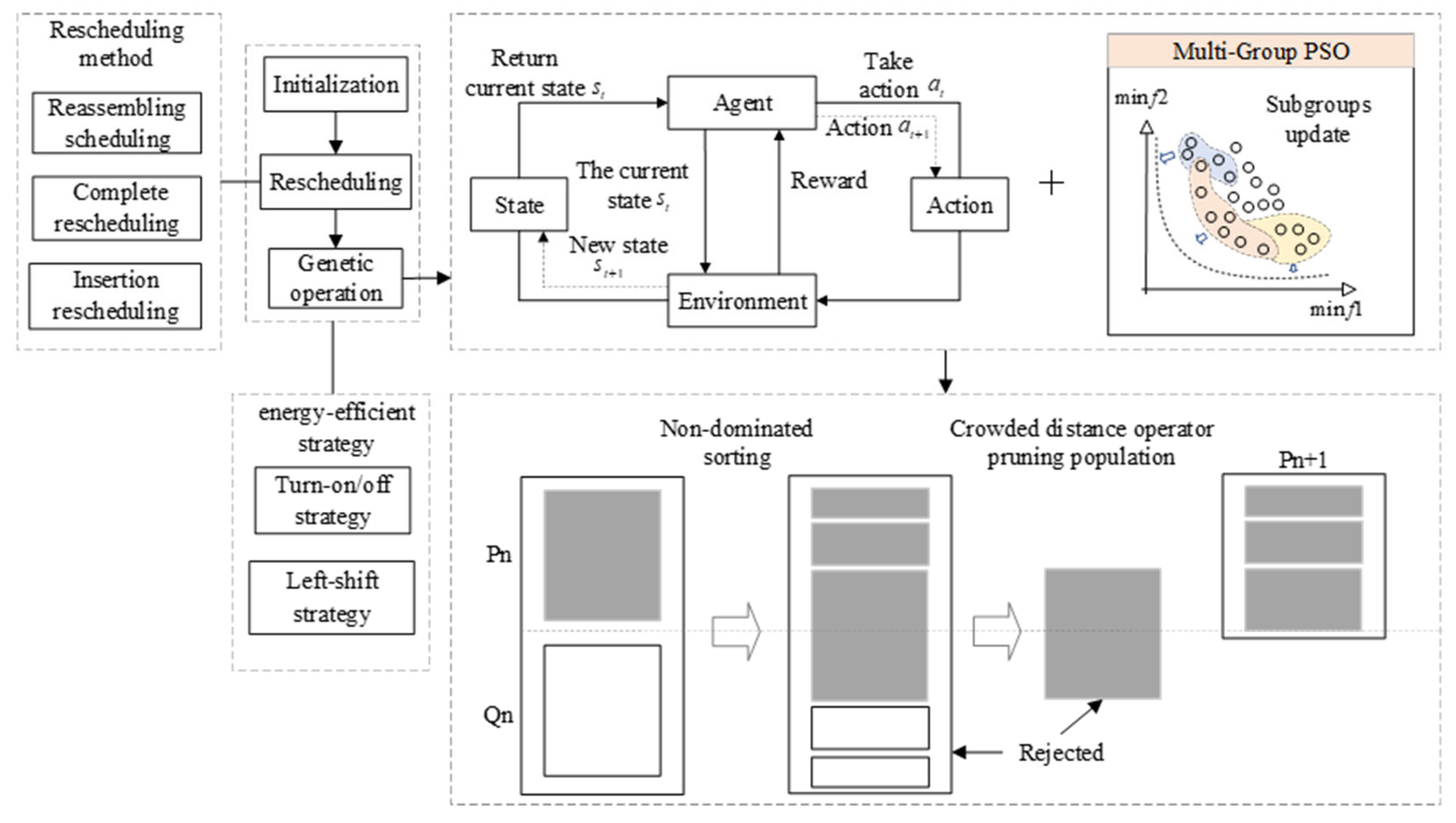
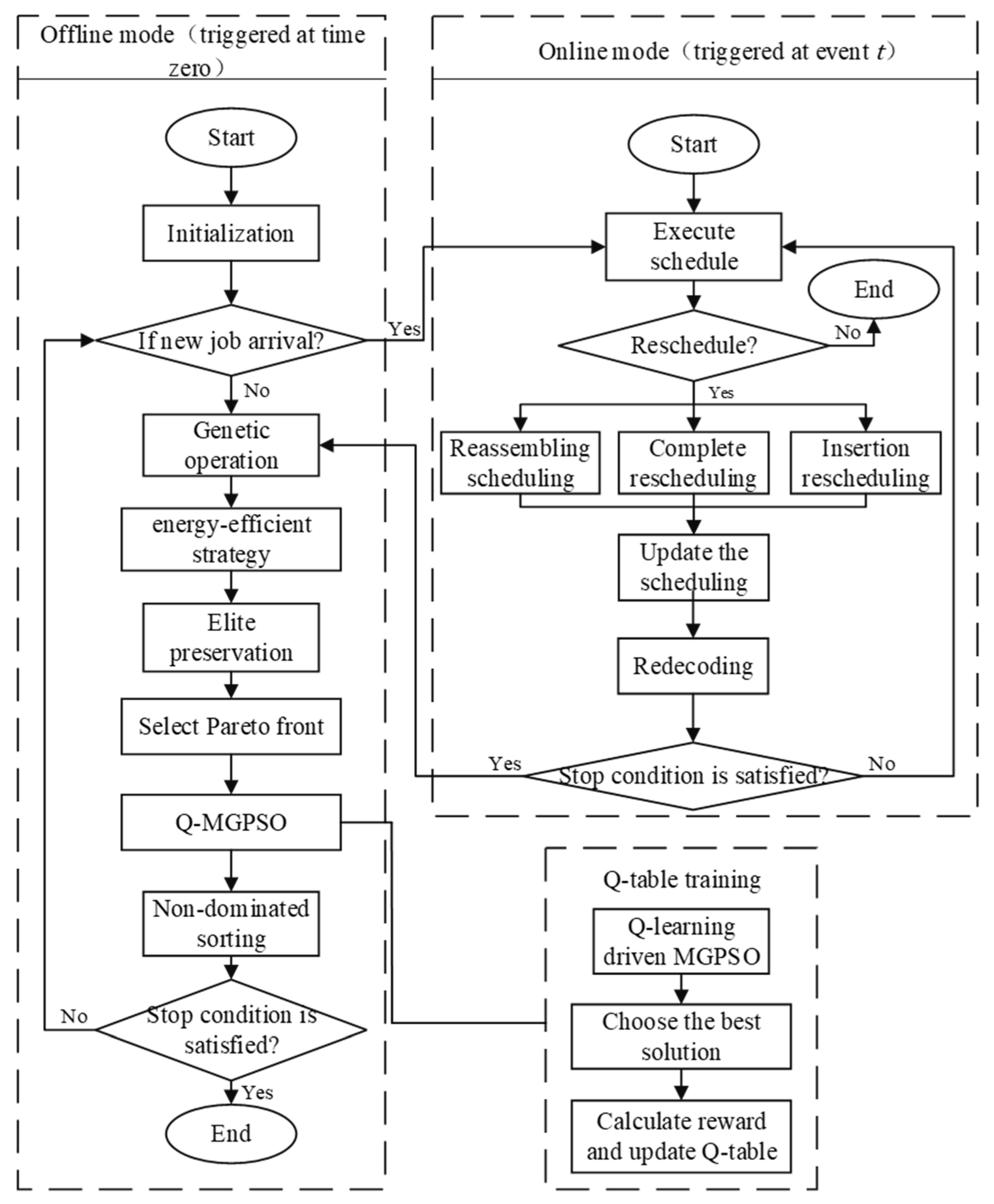
2.2. Rescheduling Strategies

Unlike the research by Zhang et al. [27], this paper adopts three rescheduling methods combined with dynamic strategies to address the new job arrival problem. The descriptions of the three dynamic rescheduling methods are as follows:

• Reassembling scheduling: When new jobs arrive, the original schedule is preserved, but the system dynamically selects the optimal machine based on real-time load balancing and future time-unit predictions.
• Complete rescheduling: This method reorganizes all pending tasks and new jobs upon events rather than fixed intervals. It employs heuristics to dynamically adjust task assignments based on real-time device availability and delay risks, leveraging sliding window convolution for future gap detection.
• Insertion rescheduling: By leveraging sliding window algorithms, the system identifies idle time slots on each machine. New tasks are inserted into the earliest feasible slot to reduce makespan.

The expression for the robustness metric $S_{min}$ of the rescheduling strategy is as follows [28]:

$$S_{min}={\displaystyle \frac{\sum _{i=1}^n\sum _{j=1}^{O_{ij}}{T}_{i,j}}{\sum _{i=1}^n{O}_{ij}}}$$

(19)

$$T_{i,j}=\left\{\begin{array}{c}1, if both O_{ij}^{pre} and K_j of O_{ij} are changed \hfill \\ 0.5, if one of the O_{ij}^{pre} and K_j changs\hfill \\ 0, if both O_{ij}^{pre} and K_j of O_{ij} remain same \hfill \end{array}\right.$$

(20)

where $T_{i,j}$ represents the instability coefficient, the value of ${ T}_{i,j}$ is subject to two variables, that is, the machining machine $K_j$ of the operation ${ O}_{ij }$ and the previous operation ${ O}_{ij}^{pre}$ on the same machine ${ K}_j$.

2.3. Energy-Efficient Strategy

Based on the founded MINLP model and the attributes of TDEHFSP, the “left-shift” strategy and turn-on/off strategy are proposed to reduce TEC. For the “left-shift” strategy, during solution decoding, a temporal gap utilization strategy is implemented by analyzing the idle periods ${\mathrm{k}}_{\mathrm{j}}^{\mathrm{i}\mathrm{d}\mathrm{l}\mathrm{e}}\mathrm{o}\mathrm{f} \mathrm{m}\mathrm{a}\mathrm{c}\mathrm{h}\mathrm{i}\mathrm{n}\mathrm{e} {\mathrm{k}}_{\mathrm{j}}$ assigned to operation ${\mathrm{O}}_{\mathrm{i}\mathrm{j}}$ and its predecessor’s completion time ${\mathrm{T}}_{\mathrm{i}(\mathrm{j}-1)}$. Candidate scheduling gaps ${\mathrm{I}}_{{\mathrm{k}}_{\mathrm{j}}}\left(\mathrm{h}\right),\left(\mathrm{h}\in \left[1,{\mathrm{N}}_{{\mathrm{k}}_{\mathrm{j}}}\right]\right)$ are dynamically generated, with operation ${\mathrm{O}}_{\mathrm{i}\mathrm{j}}$ inserted into ${\mathrm{I}}_{{\mathrm{k}}_{\mathrm{j}}}\left(\mathrm{h}\right)$ only if the condition ${\mathrm{I}}_{{\mathrm{k}}_{\mathrm{j}}}^{\mathrm{s}}\left(\mathrm{h}\right)+t_{ij}^{proc}+t_{ij}^{trans} \le {\mathrm{I}}_{{\mathrm{k}}_{\mathrm{j}}}^{\mathrm{e}}\left(\mathrm{h}\right)$ is satisfied, where $t_{ij}^{proc}$ and $t_{ij}^{trans}$ denote processing and transportation durations. This mechanism optimizes both $\mathrm{T}\mathrm{E}\mathrm{C}$ and ${\mathrm{C}}_{\mathrm{m}\mathrm{a}\mathrm{x}}$ by leveraging idle machine intervals.

The “left shift” approach decreases the machine’s idle waiting time, while the turn-on/off method plays a crucial role [29] minimizes the energy used by unavoidable machine idle waiting time. When the energy consumption during machine standby idling exceeds that of turning the machine off and back on, the optimal choice is to temporarily shut down the machine and restart it just before the next job is dealt with. Instead, the machine is kept in standby mode.

3. Q-MGCOA Algorithm

To address the proposed mathematical model, this study combines Q-learning’s learning mechanism with multi-group optimization, proposing the Q-MGCOA algorithm to dynamically select search operators. Figure 2 illustrates the overall architecture of the proposed algorithm.

3.1. Encoding and Decoding

The coding scheme for the TDEHFSP problem needs to include four decisions: job sequencing, machine assignment, transport vehicles assignment, and machine switch selection. To address these needs, an effective coding scheme is employed that encompasses arrangement, ordering, and turn-on/off decision determinations throughout every phase. The coding scheme encodes only the sequence of jobs π = {1,2,…,n} and uses list scheduling (LS) to generate job alignments for subsequent stages.

LS allocates tasks to machines and transporters using the Earliest Completion Time (ECT) strategy. It is important to note that in a unified parallel machine setup, the ECT approach generates distinct scheduling outcomes based on the first available machine (FAM) principle. Even when a job is directed to the first available machine and transporter, its completion time may still exceed the ECT-predicted value due to variations in processing speeds across uniform parallel machines. Under the LS framework, jobs are sequentially processed, with each task assigned to the machine and transporter at the earliest available completion time. This mechanism inherently aligns with the intention to minimize the total makespan. The job list for subsequent stages is dynamically updated based on the completion times of tasks from prior stages.

The active decoding process in this study incorporates two distinct methodologies: initial decoding and rescheduling decoding. The decoding method discussed above corresponds to the initial decoding phase, which constructs a full scheduling plan. Rescheduling decoding serves as an extension of the initial approach, specifically designed to handle adjustments following dynamic events such as unexpected task arrivals or machine failures.

3.2. Initialization

This section presents a novel NEH-based initialization method tailored for the TDEHFSP. Unlike traditional NEH algorithms [30] that focus solely on minimizing makespan, our approach integrates multi-objective optimization by simultaneously considering $C_{max}$ and TEC. The initialization process consists of two distinct steps:

Step 1: Dual-Objective Initial Population Generation.

Objective 1: Generate an individual using $C_{max}$ as the minimization target, following the classic NEH heuristic.

Objective 2: Generate another individual using TEC as the minimization target, incorporating energy-aware scheduling rules. This dual-objective approach ensures a diverse initial population that balances efficiency and sustainability.

Step 2: Residual Population Construction.

The remaining individuals in the population are randomly generated to maintain genetic diversity. This step prevents premature convergence and enhances the algorithm’s exploration capability.

3.3. Genetic Operation and Elite Preservation

Evolutionary processes, such as recombination and variation, serve as the foundation for investigating the feasible region and averting suboptimal local solutions. Because of the ordered nature of job sequences, this paper uses two-point order crossover and swap sequence mutations that have been widely used in HFSP.

The assessment of multi-solution quality utilizes rapid non-dominated sorting (FNS) and congestion distance estimation to formulate the Pareto dominance comparator for solution evaluation. The operators “≺” and “≻” symbolize “less optimal” and “more optimal”, respectively. In minimization-focused problems, a reduced objective value equates to an improved solution, and conversely.

Definition 1.

If a solution $x_1$Pareto is better than another solution${ x}_2$, it obeys

$$f_j\left(x_1\right)\prec f_j\left(x_2\right),\forall j\in \left\{\mathrm{1,2},3\cdots \right\}.$$

(21)

Definition 2.

If a solution $i$is better than $j$, it obeys

$$i{\prec }_n:if\left(i_{rank}<j_{rank}\right)or\left(i_{rank}=j_{rank} and{ i}_{distance}>j_{distance}\right),$$

(22)

where $i_{rank }$ and ${ i}_{distance}$ are the solution rank and congestion distance, respectively. $f_j\left(\cdot \right)$ is the objective function.

3.4. Neighborhood Structure and Local Search

In the proposed Q-MGCOA algorithm, the search process is driven by Q-learning integrated into the multi-group particle swarm optimization (MGPSO) framework, which selects the most suitable search operators during the evolutionary process [8]. To adjust the search range and strategy of the particles in real-time, a simple perturbation operator is introduced as the neighborhood structure, i.e., Destruction–Construction (DC). In addition, the MGPSO extends the velocity update equation to include a collaborative archive mechanism to facilitate information exchange between subpopulations.

Adopting a collaborative archive mechanism in local search, where particles refer to solutions in the archive to adjust their positions and velocities, facilitates information exchange between subpopulations and further enhances the efficacy of localized search. The local search operator is key to improving the method. This paper uses three search operators, namely critical swap (CSwap), critical insertion (CInsr), and critical inverse (CInv).

The MGPSO extended velocity update equation can be stated as

$$\begin{array}{c}{V}_i\left(t+1\right)=\omega V_i\left(t\right)+c_1{r}_1\left(y_i\left(t\right)-x_i\left(t\right)\right)+{{\lambda }_{i}c}_2{r}_2\left({\widehat{y}}_i\left(t\right)-x_i\left(t\right)\right)\\ +(1-{\lambda }_i)c_3{r}_3({\widehat{a}}_i\left(t\right)-x_i\left(t\right)),\end{array}$$

(23)

In this equation, $V_i\left(t\right)$ denotes the velocity of particle $i$ at iteration $t$, $\omega$ represents the inertia weight $c_1$, $c_2$, and $c_3$ symbolize acceleration coefficients, and $r_1$, $r_2$, and $r_3$ are arbitrary vectors with components uniformly distributed between 0 and 1. The terms $x_i\left(t\right)$ and $y_i\left(t\right)$ i signify the position of particle $i$ and its optimal position at iteration $t$-th, respectively. Furthermore, ${\widehat{y}}_i\left(t\right)$ and ${\widehat{a}}_i\left(t\right)$ are the global best position and neighborhood optimal position, respectively, while ${\lambda }_i$ stands for the exploitation trade-off coefficient associated with particle $i$.

This study redefines the state and action sets of Q-learning. The state set S1 represents different motion modes and damage–construction strategies of the particle swarm. For example, different inertia weights, velocity updating rules, and DC strategies can form the state set $S_1$, denoted as $S_1=\{{IW}_1,{IW}_2, \dots ,{IW}_N, D_1, D_2, \dots ,D_M\}$. On the other hand, the set of states represents different methods of local search operations, i.e., $S_2$= {CSwap, CInsr, CInv,}. The action set is the same as the state set, i.e., $A_1$ $=$ $S_1$ and $A_2=$ $S_2$. For detailed information, refer to Figure 3.

To address multiple objectives in reward allocation, the reward function is adapted to a multi-objective version through normalization, together with the total number. The new reward function not only considers the improvement of the objective function but also introduces the investigation of the improvement of the method in the archive. Specifically, the reward function can be stated as

$$r_t=\sum _k{\displaystyle \frac{f_k^{min}}{f_k\left(x_t\right)}}\left({\displaystyle \frac{f_k\left(x_t\right)-f_k\left(x_{t+1}\right)}{f_k^{max}-f_k^{min}}}\right)+\beta \times {∆}_{archive} ,$$

(24)

where $x_t$ is the solution at time t, and $x_{t+1}$ is the new solution. $f_k( )$ denotes the $k$-th objective function, $f_k^{max}$ and $f_k^{min}$ are the worst and best values of the currently found $k$-th objective function, respectively. ${∆}_{archive}$ denotes the improvement of the new solution on the set of solutions in the archive, and $\beta$ is the moderating factor.

Algorithm 1 is the detailed procedure of MGPSO with Q-learning, made up of two steps. Step 1 is particle search and Q1 training. Evaluate the new position of each particle perturbation and update the Q1 table. Step 2 is the local search and Q2 training phase, which utilizes the collaborative archive to guide the local search and update Q2.

Algorithm 1: MGPSO with Q-Learning process

Input: parameters learning factor $\alpha$, discount factor $\gamma$, Epsilon-greedy factor $\epsilon$, initial solution $x_0$, state set $S_1$, $S_2$, action set $A_1$, $A_2$, the number of episodes $E$, Non-progressing iterations highest number: Iter_Max Output: Best solution $x^{\mathrm{*}}$, Q-tables Q1, Q2 1: Initialise Q-tables Q1, Q2 as zero matrices 2: Initialise global best solution $x^{\mathrm{*}}$ = $x_0$ 3: Divide particles into $M$ subpopulations 4: Initialise particle positions and velocities Initialise personal best positions pi for each particle Initialise neighbourhood structure for each particle # Particle Search and Q1 Training 5: For $t=1$: Max-iter do 6:  For each subpopulation m in $1:M$ do 7:    For each particle $i$ in subpopulation $m$ do 8:      Select action $a_1$ from $A_1$ using Epsilon-greedy(Q1) 9:      Apply Destruction-Construction to particle $i$ based on $a_1$ 10:      Evaluate new position $x_i\mathrm{\prime }$ 11:      Update personal best position pi if $x_i\mathrm{\prime }$ is better 12:      Calculate reward $r$ 13:      Update Q1 using Q-learning $(\alpha ,\gamma ,s_1,a_1,r)$ 14:    End for 15:  End for # Local Search and Q2 Training 16:  Identify and update global best solution $x^{\mathrm{*}}$ 17:  Update collaborative archive with new non-dominated solutions 18:  For each particle $i$ in $1:P$ do 19:    Select action $a_2$ from $A_2$ using Epsilon-greedy(Q2) 20:    Apply local search operator to particle $i$ based on $a_2$ 21:    Evaluate new position $x_i\mathrm{\prime }$ 22:    Update personal best position pi if $x_i\mathrm{\prime }$ is better 23:    Calculate reward $r$ 24:    Update Q2 using Q-learning $(\alpha ,\gamma ,s_2,a_2,r)$ 25:  End for # Update Velocity and Position 26:  For each particle $i$ in $1:P$ do 27:    Update velocity $v_i$ and position $x_i$ using PSO equations and collaborative archive 28:  End for # Check for Stopping Criteria 29:  If no improvement in $x^{\mathrm{*}}$ for Max-iter iterations then 30:    Break 31:  End if 32: End for 33: Return best solution $x^{\mathrm{*}}$

The complexity of DC is $O (d+dn\sum _{j=1}^s{l}_j)$, $\sum _{j=1}^s{l}_j$ signifies the machine number. The worst-case complexity of the Q-learning process is $O \left(d_{max}\right)$. The complexity of the three local search operators in computing the critical path is $O \left(n\sum _{j=1}^s{l}_j\right)$. The complexity of the Q-learning update is $O (3$). So, the total complexity is $O \left(E\right(d+dn\sum _{j=1}^s{l}_j+d_{max}+n\sum _{j=1}^s{l}_j+3)$. The simplified complexity is $O \left(n\sum _{j=1}^s{l}_j\right)$.

The Q-MGCOA algorithm proposes an event-triggered reinforcement learning rescheduling model for dynamic events, integrating offline and online modes to address static scheduling and dynamic scheduling with new job arrivals, respectively. For the offline mode, an MGPSO algorithm based on perturbation operators and a Q-learning-driven mutation mechanism is employed to drive population evolution while transitioning to the online mode upon detecting dynamic events. In the online mode, three rescheduling heuristic algorithms are activated to respond to dynamic events and adaptively adjust the original scheduling. The complete workflow is illustrated in Figure 4.

4. Experiment Validation and Result Analysis

This section generates benchmark test instances of the TDEHFSP problem, followed by systematic experimentation of parameter adjustments identifies crucial parameters of Q-MGCOA.

4.1. Experiment Settings

Due to scarce prior research on TDEHFSP benchmark instances, random test cases were produced. Instances follow the format “jobs-stages-machines per stage-new job arrivals”. For instance, 10-3-4-2 represents 10 jobs, 3 stages, 4 machines each, and 2 new job arrivals, and 3 new job arrivals, expressed as “10-3-4-3”. These instances are abstracted from the manufacturing process of container production—specifically, the assembly of containers. The simplified process includes five stages: material preparation, cutting, welding (machine welding and manual touch-up), assembly, and painting.

Table 2. Test example parameter settings (Zhang et al. [26]).

Factors	Levels
Sum of jobs	{10, 20, 50}
Sum of stages	{3, 5}
Sum of machines per stage	{3, 4, 5}
Number of new jobs arrived	{3, 5}
Number of transport vehicles per stage	2
Processing time per operation	$U$ (20, 30) min
Power of machine	$U$ (5, 10) $\times {10}^3$ W
Speed of no-load/load transport vehicles	30\20 m/min
Power of no-load/load transport vehicles	100\200 W
Standby power of the machine	2
Reset power of the machine	4

provides the experimental setup (Zhang et al. [26]).

The parameter settings in the present study are based on classic research in the field of hybrid flow shop scheduling (Luo et al. [31]), as these scales effectively balance computational complexity and the diversity of real-world production scenarios.

4.2. Evaluation Indicators

GD, IGD, and Spread are adopted to evaluate the convergence, comprehensiveness, and distribution uniformity of Pareto fronts, respectively. These metrics are widely used in multi-objective optimization to holistically assess algorithm performance.

Spacing Matrix (SM): A lower value of SM shows a more equitable distribution of solutions of Pareto frontier solutions. The formula is as follows:

$$SM=\sqrt{{\displaystyle \frac{{\sum }_{i=1}^A(d_{min}^i-\overline{d_{min}^i}{)}^2}{\left|A\right|}}} ,$$

(25)

where $d_{min}^i$ represents the minimal aggregation of absolute discrepancies in standardized goal function outputs of the $i$-th solution in the obtained non-dominated set A and any other solution, and $\overline{d_{min}^i}$ denotes the average value of $d_{min}^i$.

Generation Distance (GD) represents the average distance between the obtained Pareto front ($PFa$) and the actual Pareto front (${PF}^{*}$), reflecting the degree of proximity between them. The formula is as follows:

$$GD={\displaystyle \frac{\sqrt{\sum _{i=1}^{n_{PFa}}{d}_i^2}}{n_{PFa}}},$$

(26)

where $d_i$ signifies the smallest Euclidean distance between the $i$-th individual in $PFa$ and an individual in ${PF}^{*}$. While $n_{PFa}$ is the count of individuals in $PFa$. This study employs the maximum minimization technique for normalization, with ${PF}^{*}$ symbolizing the combined Pareto front derived from all algorithms in the given scenario. The max–min normalization technique scales objective values to [0, 1] for fair comparison across heterogeneous objectives. Compared to Z-score normalization, this method reduces computational instability.

The inverse generational distance (IGD) serves as an inclusive metric for assessing the aggregation and variability dimensions of a resolution collection produced by an algorithm. The expression is below:

$$IGD={\displaystyle \frac{\sum _{i=1}^{n_{P{F}^{\mathrm{*}}}}{d}_i^{\mathrm{*}}}{n_{{PF}^{\mathrm{*}}}}}$$

(27)

where $d_i^{\mathrm{*}}$ is the smallest Euclidean distance between the $i$-th solution in $P{F}^{\mathrm{*}}$ and an individual in $PFa$. $n_{P{F}^{\mathrm{*}}}$ is the number of individuals in $P{F}^{\mathrm{*}}$.

The spatial metric (Spread) quantifies the dispersion of solutions along the Pareto front, indicating the variety within the acquired set. A reduced Spread value implies a more even dispersion of outcomes, thereby suggesting enhanced diversity in the solution set generated by the optimization method. The expression is as follows:

$$Spread={\displaystyle \frac{d_f+d_l+{\sum }_{i=1}^{n-1}|d_i^{i+1}-\overline{d_i^{i+1}|}}{d_f+d_l+\left(n-1\right)\overline{d_i^{i+1}}}},$$

(28)

Here, $d_f$ represents the Euclidean distance between the smallest and largest objective function values in the obtained set, while $d_l$ signifies the distance from the nearest solution to the true Pareto frontier. $d_i^{i+1}$ is the Euclidean distance between adjacent solutions within the set, and $\overline{d_i^{i+1}}$ is the mean distance across neighboring solution pairs.

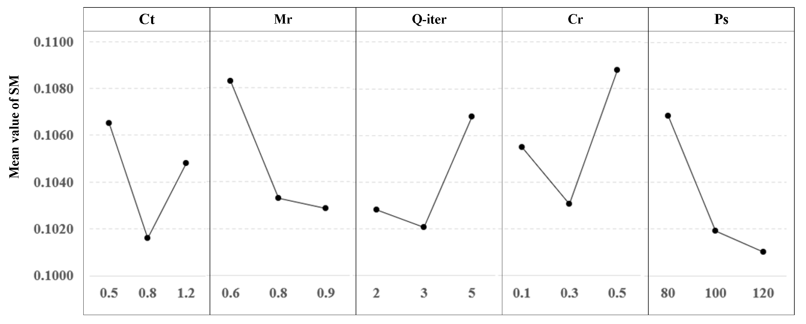
4.3. The Result of Parameter Tuning

To obtain the optimal parameter combination more quickly, we set up three groups of parameter combinations (low, medium, high) for the Taguchi experiment, including termination threshold (Q-$iter$), population size ($Ps$), mutation rate ($Mr$), crossover rate ($Cr$), and computational budget coefficient (Ct). The orthogonal array of parameter settings is shown in

Table 3. Parameter levels (Zhang et al. [26]).

Factors	Factor Levels
	1	2	3
$Ct$	0.5	0.8	1.2
$Mr$	0.6	0.8	0.9
Q-$iter$	2	3	5
$Cr$	0.1	0.3	0.5
$Ps$	80	100	120

, with five factors selected, each at three levels (Zhang et al. [26]). Peize et al. [24] obtained the optimal parameter settings for solving this type of problem as follows: the number of generations $Max\_Gen=100$, learning factor $\alpha =0.1,$ offset factor $\epsilon =0.1$, discounting factor $\lambda =0.1$, and maximum DC depth is 8.

Parametric analysis in Figure 5 demonstrates the dominant influences of Ct and Q-$iter$ over $Ps$ on optimization performance for the 20-3-3-3 instance. The calibrated Q-MGCOA configuration achieves optimality at $Ps=120$, $Mr=0.9$, $Cr=0.3$, $Q$-$iter=3$, and $Ct=0.8$. Benchmark tests enforce standardized settings: uniform genetic operators, $Ps=120,$ and $Ct\times n\times m$ termination criterion to ensure equitable comparisons.

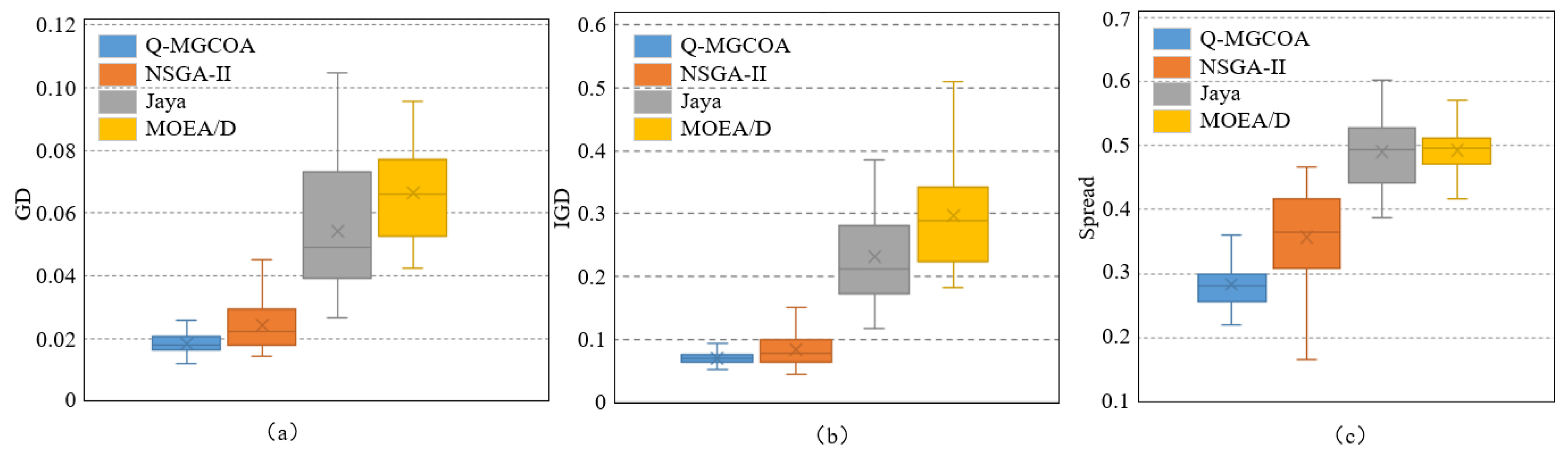
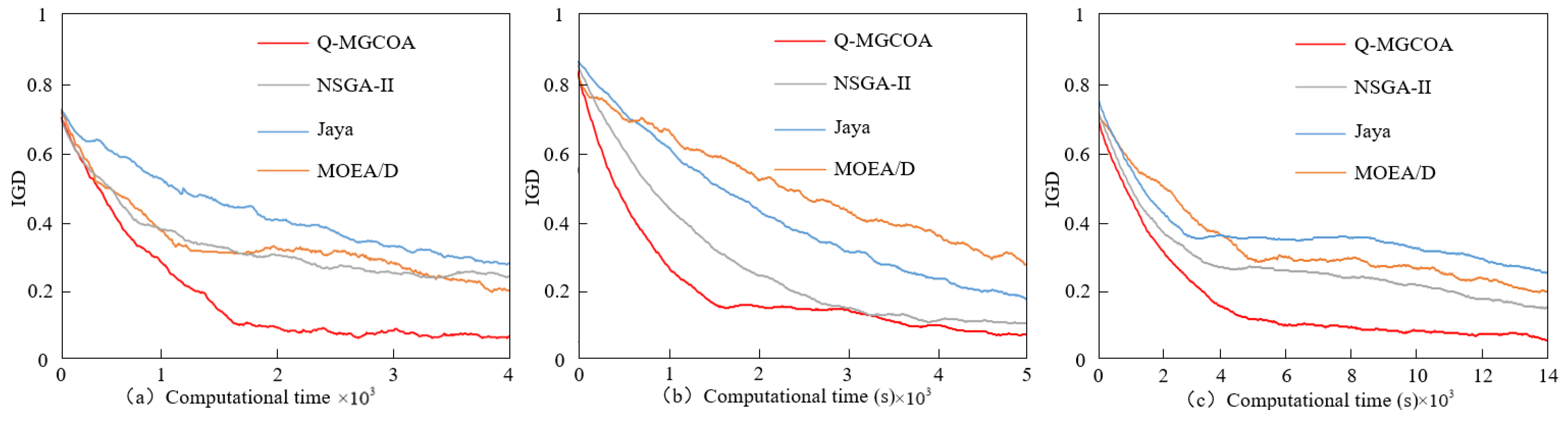
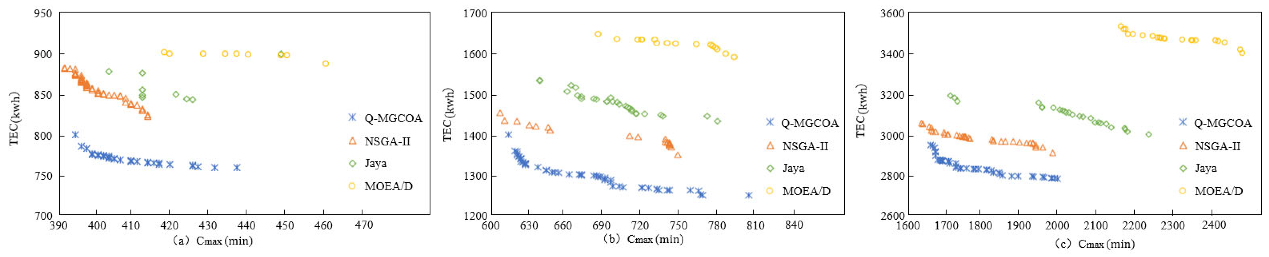
4.4. Algorithm Comparison and Analysis

Contrasting Q-MGCOA with traditional NSGA-II [25] and multi-objective evolutionary algorithms (MOEAs) like improved Jaya [32] and MOEA/D [33]. Reveals performance differences in optimization tasks.

Across the 36 produced scenarios, every algorithm underwent execution independently for five iterations. The AVG and STD of the evaluation metrics GD, IGD, and Spread were computed for each algorithm. The analysis outcomes are presented in

Table 4. The analysis outcome of GD.

	NSGA-II		Jaya		MOEA/D		Q-MGCOA
	AVG	STD	AVG	STD	AVG	STD	AVG	STD
10-3-3-3	0.0196	0.0084	0.0372	0.0071	0.0614	0.0179	0.0253	0.0082
10-3-3-5	0.0239	0.0066	0.0404	0.0239	0.0484	0.0155	0.0384	0.0209
10-3-4-3	0.0269	0.0051	0.0573	0.0277	0.0457	0.0136	0.0187	0.0034
10-3-4-5	0.0290	0.0123	0.0763	0.0255	0.0614	0.0191	0.0218	0.0022
10-3-6-3	0.0624	0.0138	0.0406	0.0206	0.0552	0.0104	0.0205	0.0113
10-3-6-5	0.0236	0.0051	0.0397	0.0179	0.0716	0.0400	0.0185	0.0039
10-5-3-3	0.0678	0.0630	0.0858	0.0412	0.0531	0.0070	0.0164	0.0021
10-5-3-5	0.0332	0.0145	0.0616	0.0255	0.0501	0.0186	0.0232	0.0078
10-5-4-3	0.0208	0.0054	0.1047	0.0627	0.0515	0.0238	0.0232	0.0084
10-5-4-5	0.0204	0.0064	0.0459	0.0200	0.1732	0.1732	0.0189	0.0020
10-5-6-3	0.0449	0.0364	0.0649	0.0372	0.0770	0.0586	0.0207	0.0022
10-5-6-5	0.0295	0.0064	0.0745	0.0572	0.1732	0.1732	0.0147	0.0021
20-3-3-3	0.0168	0.0050	0.0272	0.0055	0.0611	0.0463	0.0175	0.0028
20-3-3-5	0.0176	0.0026	0.0265	0.0059	0.0659	0.0602	0.0191	0.0068
20-3-4-3	0.0158	0.0033	0.0344	0.0064	0.0661	0.0604	0.0177	0.0032
20-3-4-5	0.0184	0.0038	0.0451	0.0170	0.0641	0.0204	0.0173	0.0023
20-3-6-3	0.0225	0.0079	0.0465	0.0256	0.0476	0.0288	0.0185	0.0022
20-3-6-5	0.0252	0.0088	0.0534	0.0254	0.0424	0.0119	0.0309	0.0101
20-5-3-3	0.0389	0.0318	0.0459	0.0141	0.0771	0.0209	0.0179	0.0033
20-5-3-5	0.0293	0.0153	0.0454	0.0133	0.0734	0.0570	0.0166	0.0032
20-5-4-3	0.0305	0.0083	0.0747	0.0277	0.0765	0.0552	0.0215	0.0044
20-5-4-5	0.0216	0.0050	0.0643	0.0267	0.0956	0.0612	0.0206	0.0045
20-5-6-3	0.0213	0.0032	0.0401	0.0316	0.1183	0.0335	0.0162	0.0039
20-5-6-5	0.0292	0.0081	0.1732	0.1732	0.0551	0.0251	0.0184	0.0049
50-3-3-3	0.0150	0.0045	0.0516	0.0227	0.0910	0.0522	0.0177	0.0038
50-3-3-5	0.0162	0.0021	0.0757	0.0571	0.1081	0.0477	0.0176	0.0051
50-3-4-3	0.0260	0.0082	0.0386	0.0054	0.0749	0.0250	0.0172	0.0039
50-3-4-5	0.0192	0.0073	0.0580	0.0288	0.0662	0.0175	0.0159	0.0035
50-3-6-3	0.0162	0.0039	0.0390	0.0125	0.0672	0.0175	0.0151	0.0077
50-3-6-5	0.0144	0.0022	0.0539	0.0243	0.0522	0.0194	0.0134	0.0013
50-5-3-3	0.0219	0.0048	0.0781	0.0563	0.0732	0.0273	0.0132	0.0039
50-5-3-5	0.0217	0.0072	0.0368	0.0072	0.0674	0.0138	0.0160	0.0018
50-5-4-3	0.0282	0.0101	0.1732	0.1732	0.0801	0.0578	0.0169	0.0033
50-5-4-5	0.0170	0.0045	0.0358	0.0095	0.0476	0.0153	0.0125	0.0018
50-5-6-3	0.0158	0.0044	0.0312	0.0058	0.0912	0.0496	0.0121	0.0013
50-5-6-5	0.0248	0.0114	0.0782	0.0534	0.0507	0.0161	0.0204	0.0122
Hit rate	9/36	8/36	0/36	0/36	0/36	0/36	27/36	28/36

,

Table 5. The analysis outcome of IGD.

	NSGA-II		Jaya		MOEA/D		Q-MGCOA
	AVG	STD	AVG	STD	AVG	STD	AVG	STD
10-3-3-3	0.0438	0.0061	0.1414	0.0303	0.2610	0.0717	0.0696	0.0045
10-3-3-5	0.0821	0.0211	0.1818	0.1108	0.2132	0.0706	0.1240	0.0392
10-3-4-3	0.0898	0.0388	0.2151	0.1456	0.2077	0.0697	0.0797	0.0192
10-3-4-5	0.0783	0.0336	0.3230	0.1192	0.2984	0.1078	0.0724	0.0100
10-3-6-3	0.0436	0.0106	0.1348	0.0501	0.2470	0.0769	0.0546	0.0195
10-3-6-5	0.0649	0.0130	0.1742	0.0908	0.2939	0.1698	0.0633	0.0171
10-5-3-3	0.2684	0.3571	0.3379	0.1383	0.2118	0.0627	0.0637	0.0074
10-5-3-5	0.1182	0.0644	0.2754	0.1194	0.2219	0.0853	0.0924	0.0295
10-5-4-3	0.0630	0.0201	0.5256	0.3428	0.2248	0.1433	0.0828	0.0232
10-5-4-5	0.0678	0.0142	0.1907	0.0672	0.9000	0.9000	0.0790	0.0055
10-5-6-3	0.1144	0.1033	0.2749	0.1819	0.3808	0.3120	0.0698	0.0088
10-5-6-5	0.0880	0.0334	0.3570	0.3119	0.9000	0.9000	0.0543	0.0033
20-3-3-3	0.0598	0.0211	0.1173	0.0279	0.2583	0.1792	0.0669	0.0146
20-3-3-5	0.0761	0.0217	0.1221	0.0304	0.3086	0.3312	0.0832	0.0302
20-3-4-3	0.0670	0.0159	0.1604	0.0390	0.3145	0.3283	0.0704	0.0158
20-3-4-5	0.0527	0.0043	0.1962	0.0974	0.2874	0.0833	0.0599	0.0095
20-3-6-3	0.0870	0.0322	0.2120	0.1345	0.2098	0.1350	0.0677	0.0139
20-3-6-5	0.0716	0.0333	0.2224	0.1197	0.1825	0.0491	0.1247	0.0544
20-5-3-3	0.1500	0.1264	0.2209	0.0647	0.3240	0.0845	0.0728	0.0151
20-5-3-5	0.1300	0.0855	0.1845	0.0688	0.3514	0.3114	0.0715	0.0163
20-5-4-3	0.1202	0.0315	0.3405	0.1305	0.3656	0.3022	0.0819	0.0282
20-5-4-5	0.0875	0.0102	0.2852	0.1302	0.4374	0.3031	0.0867	0.0239
20-5-6-3	0.0983	0.0206	0.1830	0.1516	0.5681	0.1927	0.0657	0.0109
20-5-6-5	0.1084	0.0303	0.9000	0.9000	0.2380	0.1072	0.0717	0.0245
50-3-3-3	0.0611	0.0222	0.2466	0.1233	0.4474	0.2762	0.0711	0.0136
50-3-3-5	0.0576	0.0063	0.3677	0.3066	0.5104	0.2527	0.0705	0.0201
50-3-4-3	0.0976	0.0364	0.1773	0.0313	0.3253	0.1463	0.0740	0.0132
50-3-4-5	0.0723	0.0204	0.2678	0.1182	0.2776	0.0697	0.0657	0.0160
50-3-6-3	0.0633	0.0216	0.1867	0.0710	0.2880	0.0862	0.0607	0.0341
50-3-6-5	0.0619	0.0122	0.2538	0.1252	0.2183	0.0759	0.0561	0.0070
50-5-3-3	0.0917	0.0253	0.3859	0.2989	0.3329	0.1387	0.0562	0.0201
50-5-3-5	0.0940	0.0322	0.1652	0.0367	0.3044	0.0736	0.0675	0.0077
50-5-4-3	0.1259	0.0453	0.9000	0.9000	0.3886	0.3059	0.0701	0.0173
50-5-4-5	0.0734	0.0247	0.1688	0.0510	0.2128	0.0755	0.0549	0.0110
50-5-6-3	0.0646	0.0153	0.1562	0.0284	0.4282	0.2778	0.0524	0.0065
50-5-6-5	0.1094	0.0576	0.3813	0.2926	0.2245	0.0670	0.0858	0.0503
Hit rate	11/36	10/36	0/36	0/36	0/36	0/36	25/36	26/36

and

Table 6. The analysis outcome of the Spread.

	NSGA-II		Jaya		MOEA/D		Q-MGCOA
	AVG	STD	AVG	STD	AVG	STD	AVG	STD
10-3-3-3	0.3013	0.0928	0.4808	0.0739	0.5019	0.0256	0.2482	0.0227
10-3-3-5	0.2856	0.0383	0.3869	0.0783	0.5320	0.0338	0.4257	0.0262
10-3-4-3	0.4361	0.0736	0.4980	0.0581	0.5195	0.0519	0.2832	0.0695
10-3-4-5	0.3800	0.0922	0.5257	0.0695	0.5937	0.0370	0.2994	0.0433
10-3-6-3	0.1667	0.0393	0.4326	0.0856	0.5990	0.0460	0.1766	0.0309
10-3-6-5	0.3450	0.1039	0.4333	0.0642	0.5241	0.0786	0.2322	0.0554
10-5-3-3	0.4227	0.0814	0.4346	0.0492	0.4929	0.0387	0.2542	0.0378
10-5-3-5	0.4275	0.1076	0.5295	0.0846	0.4958	0.0702	0.2929	0.0330
10-5-4-3	0.2501	0.0557	0.4325	0.1146	0.5131	0.0167	0.2833	0.0816
10-5-4-5	0.3934	0.0649	0.5342	0.0574	0.4790	0.0971	0.2633	0.0307
10-5-6-3	0.4020	0.1018	0.4387	0.0677	0.4874	0.1029	0.3210	0.0357
10-5-6-5	0.2842	0.0376	0.4373	0.0474	0.5429	0.0491	0.1806	0.0254
20-3-3-3	0.2844	0.0949	0.4016	0.0367	0.5696	0.0467	0.2204	0.0382
20-3-3-5	0.3248	0.0462	0.4592	0.0162	0.5076	0.0728	0.2804	0.0440
20-3-4-3	0.2339	0.0495	0.4603	0.0619	0.4689	0.0607	0.2566	0.0510
20-3-4-5	0.3481	0.0452	0.5097	0.1092	0.4727	0.0543	0.3489	0.0632
20-3-6-3	0.3671	0.1033	0.5195	0.0687	0.5073	0.0664	0.2959	0.0500
20-3-6-5	0.4153	0.0563	0.5119	0.0954	0.4566	0.0506	0.3598	0.0538
20-5-3-3	0.3886	0.0970	0.5797	0.0797	0.4451	0.0575	0.2714	0.0597
20-5-3-5	0.4510	0.0516	0.4707	0.0880	0.5026	0.0990	0.2967	0.0228
20-5-4-3	0.3528	0.0487	0.4711	0.0657	0.5122	0.1099	0.3582	0.0461
20-5-4-5	0.3458	0.0835	0.4149	0.0424	0.4965	0.0907	0.3221	0.0228
20-5-6-3	0.3160	0.0518	0.5113	0.1079	0.4629	0.1117	0.2546	0.0765
20-5-6-5	0.4670	0.0570	0.5314	0.0440	0.4167	0.0327	0.2705	0.0409
50-3-3-3	0.3265	0.0624	0.4936	0.0617	0.4900	0.0653	0.3163	0.0591
50-3-3-5	0.2469	0.0363	0.4700	0.0718	0.4970	0.1210	0.2615	0.0688
50-3-4-3	0.4303	0.0389	0.5199	0.0950	0.4732	0.0334	0.2924	0.0346
50-3-4-5	0.4173	0.0824	0.5723	0.0441	0.4913	0.0622	0.2765	0.0236
50-3-6-3	0.3619	0.0620	0.5538	0.0643	0.5094	0.0323	0.2842	0.0616
50-3-6-5	0.3846	0.0403	0.5293	0.0467	0.5255	0.0560	0.2695	0.0425
50-5-3-3	0.4619	0.1154	0.5527	0.0906	0.4637	0.0493	0.2952	0.0788
50-5-3-5	0.3318	0.0547	0.5187	0.0880	0.5210	0.0688	0.2525	0.0376
50-5-4-3	0.4240	0.0690	0.4457	0.0536	0.5073	0.0859	0.3274	0.0410
50-5-4-5	0.3732	0.0719	0.4947	0.0674	0.4490	0.0942	0.2770	0.0648
50-5-6-3	0.3067	0.0369	0.6015	0.0375	0.4715	0.0607	0.2268	0.0380
50-5-6-5	0.3864	0.0490	0.4828	0.1024	0.4364	0.0534	0.2517	0.0558
Hit rate	7/36	7/36	0/36	2/36	0/36	6/36	29/36	21/36

, where bolded values indicate the best performance among the three, and the hit rate reflects how often each algorithm achieved the best results across all instances. Box plots of the GD, IGD, and Spread test results across different algorithms are displayed in Figure 6. From the GD results in Table 4, Q-MGCOA achieves 27 optimal AVGs and 28 optimal STDs, indicating that Q-MGCOA can obtain a solution set closer to the optimal Pareto boundary.

Table 4 compares the Generation Distance (GD) of NSGA-II, Jaya, MOEA/D, and Q-MGCOA across 36 scenarios. GD measures the proximity to the true Pareto front. Q-MGCOA shows superiority, achieving 27 optimal AVGs and 28 optimal STDs, indicating it can obtain a solution set closer to the optimal Pareto boundary.

Table 5 presents the inverse generational distance (IGD) analysis of four algorithms in 36 scenarios. IGD assesses solution set quality comprehensively. Q-MGCOA performs best with 25 optimal AVGs and 26 optimal STDs, suggesting it generates Pareto frontiers with better convergence and diversity.

Table 6 displays the Spread metric results for NSGA-II, Jaya, MOEA/D, and Q-MGCOA in 36 cases. Spread measures solution dispersion on the Pareto front. Q-MGCOA gets the majority of optimal AVGs and STDs, meaning its Pareto frontiers have better dispersal unification.

The boxplot in Figure 6 not only validates the aforementioned conclusions but also visually demonstrates the superiority of the proposed algorithm across the three evaluation metrics: GD, IGD, and Spread. The results show that Q-MGPSO-NSGA-II performs well across three evaluation metrics, outperforming in approximately 75%, 69%, and 81% of instances. In summary, compared to NSGA-II, Jaya, and MOEA/D, Q-MGCOA demonstrates superior overall performance, assessing the efficacy and prominence of the method for solving TDEHFSP problems.

Figure 7 visualizes the convergence performance of the algorithms by plotting the IGD values over time for three instances: 10-5-3-3, 20-5-3-3, and 50-5-3-3. The IGD metric was selected because it is a comprehensive metric. As shown in Figure 7a, Q-MGCOA converges to the minimum value faster in the small-scale instances, indicating a well-balanced global exploration and local exploitation. Figure 7b shows that Q-MGCOA slightly outperforms NSGA-II, consistent with the results in Table 6 for medium-scale instances. Additionally, Figure 7c shows that the convergence curve of Q-MGCOA is smoother than that of the other algorithms, demonstrating its robustness in solving large-scale instances. In summary, these results suggest that Q-MGCOA is more efficient in solving TDEHFSP problems.

To further evaluate the algorithm’s performance, we selected three test instances, namely 10-5-3-3, 20-5-3-3, and 50-5-3-3, for the experiments. The Pareto front comparison diagram obtained is shown in Figure 8. As shown in the image, the scheduling outcomes obtained by the Q-MGPSO algorithm demonstrate significantly lower values in both maximum makespan and total energy consumption compared to the Jaya and MOEA/D algorithms. On the other hand, while the NSGA-II algorithm can achieve a lower maximum makespan, at the same level of maximum makespan, the scheduling results produced by the Q-MGPSO algorithm reduce the total energy consumption. As shown in

Table 7. The lowest TEC (kwh) results.

$\mathbf{TEC} \left(\mathbf{k}\mathbf{w}\mathbf{h}\right)$	NSGA-II	Jaya	MOEA/D	Q-MGCOA
10-5-3-3	823	847	878	758
20-5-3-3	1348	1447	1596	1236
50-5-3-3	2908	3004	3321	2745

, the minimum energy consumption (TEC) values achieved by Q-MGCOA are 8%, 8%, and 6% lower than those of NSGA-II for the three instances. Therefore, this further confirms the efficacy of the proposed energy-saving strategies and rescheduling. Moreover, this validates that the proposed Q-MGPSO algorithm can explore more feasible solutions without losing the current optimal solutions, demonstrating strong optimization capabilities and delivering practical guidelines for smart, green container-terminal operations.

5. Conclusions

Optimizing energy-efficient job sequencing in container-oriented hybrid flow shops has become critical for container production resilience and sustainability. First, a MINLP model for the Resilient Container-supply TDEHFSP (RC-TDEHFSP) is established, jointly minimizing makespan, total energy consumption and a novel supply-chain resilience index, and an energy-efficient strategy to reduce $TEC$ without affecting productivity is proposed. To address the scheduling challenges caused by the delayed introduction of new jobs in TDEHFSP, a novel algorithm, Q-MGCOA is developed to solve this model by leveraging the strengths of multiple algorithms, ensuring adaptability and efficiency in dynamic scenarios.

To evaluate the viability of the suggested method, the optimized Q-MGCOA is compared with NSGA-II, improved Jaya, and MOEA/D in this paper. Compared to the other three algorithms, the percentage of performance dominance of Q-MGCOA on the three evaluated metrics (GD, IGD, and Spread) is about 75%, 69%, and 81% in 36 computational instances of different sizes. Moreover, it achieves about an 8% reduction in energy consumption compared to traditional algorithms. The comparative analysis reveals that the algorithm demonstrates superior performance in addressing TDEHFSP, notably outperforming the other three approaches.

Still, this study has several notable limitations. First, the scheduling framework exclusively accounts for dynamic job arrivals as the primary uncertainty factor, neglecting potential disruptions from other sources. Second, the material transfer analysis focuses solely on transport vehicles without incorporating auxiliary handling systems like overhead cranes that play vital roles in specialized production environments. Subsequent investigations should expand the model’s adaptability by integrating complementary dynamic variables and diversified material transfer mechanisms.

References

1. Wang, Y.J.; Li, J.; Wang, G.G. Fuzzy correlation entropy-based NSGA-II for energy-efficient hybrid flow-shop scheduling problem. Knowl.-Based Syst. 2023, 277, 110808. [Google Scholar] [CrossRef]
2. Wang, Z.; Shen, L.; Li, X.; Gao, L. An improved multi-objective firefly algorithm for energy-efficient hybrid flowshop rescheduling problem. J. Clean. Prod. 2023, 385, 135738. [Google Scholar] [CrossRef]
3. Goli, A.; Ala, A.; Hajiaghaei-Keshteli, M. Efficient multi-objective meta-heuristic algorithms for energy-aware non-permutation flow-shop scheduling problem. Expert Syst. Appl. 2023, 213, 119077. [Google Scholar] [CrossRef]
4. Geng, K.; Liu, L.; Wu, Z. Energy-efficient distributed heterogeneous re-entrant hybrid flow shop scheduling problem with sequence dependent setup times considering factory eligibility constraints. Sci. Rep. 2022, 12, 18741. [Google Scholar] [CrossRef]
5. Ho, M.H.; Hnaien, F.; Dugardin, F. Exact method to optimise the total electricity cost in two-machine permutation flow shop scheduling problem under Time-of-use tariff. Comput. Oper. Res. 2022, 144, 105788. [Google Scholar] [CrossRef]
6. Cui, D.; Zheng, J.; Sun, Y.; He, X.; Zhao, Z. Deploying Liquefied Natural Gas-Powered Ships in Response to the Maritime Emission Trading System: From the Perspective of Shipping Alliances. J. Mar. Sci. Eng. 2025, 13, 551. [Google Scholar]
7. Zhang, F.; Mu, H.; Wang, Z.; Chen, J.; Zhang, G.; Wang, S. A Flow Shop Scheduling Method Based on Dual BP Neural Networks with Multi-Layer Topology Feature Parameters. Systems 2024, 12, 339. [Google Scholar] [CrossRef]
8. Tao, X.R.; Pan, Q.K.; Sang, H.Y.; Gao, L.; Yang, A.-L.; Rong, M. Nondominated sorting genetic algorithm-II with Q-learning for the distributed permutation flowshop rescheduling problem. Knowl.-Based Syst. 2023, 278, 110880. [Google Scholar] [CrossRef]
9. Jiang, C.; Wang, Z.; Chen, S.; Li, J.; Wang, H.; Xiang, J.; Xiao, W. Attention-shared multi-agent actor–critic-based deep reinforcement learning approach for mobile charging dynamic scheduling in wireless rechargeable sensor networks. Entropy 2022, 24, 965. [Google Scholar] [CrossRef]
10. Luo, H.; Fang, J.; Huang, G.Q. Real-time scheduling for hybrid flowshop in ubiquitous manufacturing environment. Comput. Ind. Eng. 2015, 84, 12–23. [Google Scholar] [CrossRef]
11. Ghaleb, M.; Zolfagharinia, H.; Taghipour, S. Real-time production scheduling in the Industry-4.0 context: Addressing uncertainties in job arrivals and machine breakdowns. Comput. Oper. Res. 2020, 123, 105031. [Google Scholar] [CrossRef]
12. Khan, M.A.; Ahmed, T.; Ashraf, S.; Arfeen, Z.A. SLM-OJ: Surrogate Learning Mechanism during Outbreak Juncture. August 2022 2020, 6, 162–167. [Google Scholar]
13. Al-Hinai, N.; ElMekkawy, T.Y. Robust and stable flexible job shop scheduling with random machine breakdowns using a hybrid genetic algorithm. Int. J. Prod. Econ. 2011, 132, 279–291. [Google Scholar] [CrossRef]
14. Duan, J.; Wang, J. Robust scheduling for flexible machining job shop subject to machine breakdowns and new job arrivals considering system reusability and task recurrence. Expert Syst. Appl. 2022, 203, 117489. [Google Scholar] [CrossRef]
15. Fujimura, S.; Plazolles, B.; Luo, J.; El Baz, D. GPU based parallel genetic algorithm for solving an energy efficient dynamic flexible flow shop scheduling problem. J. Parallel Distrib. Comput. 2019, 133, 244–257. [Google Scholar]
16. Ghaleb, M.; Taghipour, S.; Zolfagharinia, H. Real-time integrated production-scheduling and maintenance-planning in a flexible job shop with machine deterioration and condition-based maintenance. J. Manuf. Syst. 2021, 61, 423–449. [Google Scholar] [CrossRef]
17. Li, W.; Gao, L.; Han, D.; Li, Y.; Li, X. Integrated production and transportation scheduling method in hybrid flow shop. Chin. J. Mech. Eng. 2022, 35, 12. [Google Scholar] [CrossRef]
18. Gong, G.; Zhao, X.; Luo, Q.; Guo, X.; Chen, L.; Deng, Q. Modelling and optimisation of distributed assembly hybrid flowshop scheduling problem with transportation resource scheduling. Comput. Ind. Eng. 2023, 186, 109717. [Google Scholar]
19. Cai, J.; Wang, J.; Wang, L.; Lei, D. A novel shuffled frog-leaping algorithm with reinforcement learning for distributed assembly hybrid flow shop scheduling. Int. J. Prod. Res. 2023, 61, 1233–1251. [Google Scholar] [CrossRef]
20. Peng, K.-K.; Gao, L.; Zhang, B.; Pan, Q.-K.; Meng, L.-L.; Li, X.-Y. A three-stage multiobjective approach based on decomposition for an energy-efficient hybrid flow shop scheduling problem. IEEE Trans. Syst. Man Cybern. Syst. 2019, 50, 4984–4999. [Google Scholar]
21. Zhang, Z.Q.; Qian, B.; Hu, R.; Yang, J.-B. Q-learning-based hyper-heuristic evolutionary algorithm for the distributed assembly blocking flowshop scheduling problem. Appl. Soft Comput. 2023, 146, 110695. [Google Scholar] [CrossRef]
22. Zhang, Z.Q.; Wu, F.C.; Qian, B.; Hu, R.; Wang, L.; Jin, H.-P. A Q-learning-based hyper-heuristic evolutionary algorithm for the distributed flexible job-shop scheduling problem with crane transportation. Expert Syst. Appl. 2023, 234, 121050. [Google Scholar] [CrossRef]
23. Jia, Y.; Yan, Q.; Wang, H. Q-learning driven multi-population memetic algorithm for distributed three-stage assembly hybrid flow shop scheduling with flexible preventive maintenance. Expert Syst. Appl. 2023, 232, 120837. [Google Scholar] [CrossRef]
24. Xue, Q.; Zhou, D.; Zhang, Z.; Chen, J.; Li, P. Multi-objective energy-efficient hybrid flow shop scheduling using Q-learning and GVNS driven NSGA-II. Comput. Oper. Res. 2023, 159, 106360. [Google Scholar]
25. Zhang, W.; Li, C.; Gen, M.; Yang, W.; Zhang, G. A multiobjective memetic algorithm with particle swarm optimisation and Q-learning-based local search for energy-efficient distributed heterogeneous hybrid flow-shop scheduling problem. Expert Syst. Appl. 2024, 237, 121570. [Google Scholar] [CrossRef]
26. Zhang, Q.; Duan, J.; Qin, J.; Zhou, Y.; Shi, H.; Nie, L.; Si, H. Double Deep Q-Network-Based Solution to a Dynamic, Energy-Efficient Hybrid Flow Shop Scheduling System with the Transport Process. Systems 2025, 13, 170. [Google Scholar] [CrossRef]
27. Zhang, W.; Gen, M.; Jo, J. Hybrid sampling strategy-based multiobjective evolutionary algorithm for process planning and scheduling problem. J. Intell. Manuf. 2014, 25, 881–897. [Google Scholar] [CrossRef]
28. Chen, X.; Li, Y.; Zhang, L.; Gao, K.; An, Y. Multiobjective flexible job-shop rescheduling with new job insertion and machine preventive maintenance. IEEE Trans. Cybern. 2022, 53, 3101–3113. [Google Scholar]
29. Li, Z.; Mumtaz, J.; Yue, L.; Wang, H.; Rauf, M. Energy-efficient scheduling of a two-stage flexible printed circuit board flow shop using a hybrid Pareto spider monkey optimisation algorithm. J. Ind. Inf. Integr. 2023, 31, 100412. [Google Scholar]
30. Meyer, P.; Mohammadi, M.; Pasdeloup, B.; Karimi-Mamaghan, M. Learning to select operators in meta-heuristics: An integration of Q-learning into the iterated greedy algorithm for the permutation flowshop scheduling problem. Eur. J. Oper. Res. 2023, 304, 1296–1330. [Google Scholar]
31. Luo, H.; Du, B.; Huang, G.Q.; Chen, H.; Li, X. Hybrid flow shop scheduling considering machine electricity consumption cost. Int. J. Prod. Econ. 2013, 146, 423–439. [Google Scholar] [CrossRef]
32. Li, Z.; Gao, K.; Wu, N.; Pan, Y. Solving biobjective distributed flow-shop scheduling problems with lot-streaming using an improved Jaya algorithm. IEEE Trans. Cybern. 2022, 53, 3818–3828. [Google Scholar]
33. Li, X.; Li, P.; Wang, G.; Gao, L. Energy-efficient distributed heterogeneous welding flow shop scheduling problem using a modified MOEA/D. Swarm Evol. Comput. 2021, 62, 100858. [Google Scholar]
Figure 1. The layout of a hybrid flow shop considering transportation processes.
Jmse 13 01153 g001
Figure 2. The overall framework of the Q-MGCOA algorithm.
Jmse 13 01153 g002
Figure 3. States S2 and actions A2 of Q-learning.
Jmse 13 01153 g003
Figure 4. The dynamic and static rescheduling model framework.
Jmse 13 01153 g004
Figure 5. Main effect plot of parameter tuning.
Jmse 13 01153 g005
Figure 6. The boxplot of GD (a), IGD (b), and Spread (c) results.
Jmse 13 01153 g006
Figure 7. The convergence curve of 10-5-3-3 (a), 20-5-3-3 (b), and 50-5-3-3 (c).
Jmse 13 01153 g007
Figure 8. The Pareto front comparison diagram of 10-5-3-3 (a), 20-5-3-3 (b), and 50-5-3-3 (c).
Jmse 13 01153 g008