Deploying Liquefied Natural Gas-Powered Ships in Response to the Maritime Emission Trading System: From the Perspective of Shipping Alliances

Abstract

In response to climate change caused by shipping, the maritime emission trading system (METS) is used to reduce ship carbon emissions, and the METS also imposes additional costs on shipping carriers through emission permit trading. This paper focuses on the deployment of liquefied natural gas-powered (LNG-powered) ships for shipping alliances to comply with the METS. From the perspective of a liner alliance, we investigate how to determine the deployment of LNG-powered ships and how ship emissions will be affected. To investigate these problems, we propose an LNG-powered fleet deployment problem, which integrates slot co-chartering and emission permit trading, to determine the fleet deployment of LNG-powered and oil-powered ships, ship speeds and container shipment. To formulate our proposed problem, we develop a mixed-integer linear programming model, which can be solved effectively by CPLEX. Numerical experiments are provided to assess the effectiveness of our proposed model.

1. Introduction

Over 70% of the global international trade volume relies on the shipping industry (UNCTAD, 2023) [1]. In the shipping industry, huge profits are accompanied by significant carbon emissions. In the decade between 2012 and 2022, carbon emissions from ships increased significantly. For container ships, RO-RO ships and passenger ships, carbon emissions grew by up to 100% [1]. In 2022, the maritime industry produced 850.6 million tons of carbon emissions, which accounts for about 2.4% of global carbon emissions. For reducing ship emissions, the regulators regard the market-based measure (MBM) as a possible pathway [2]. As a type of MBM, the maritime emission trading system (METS) has attracted the attention of industry and academia.

From 1 January 2024, the European Union is the first to implement the METS, and other countries and regions have also implemented and improved the METS to accelerate the achievement of the latest IMO greenhouse gas reduction targets, namely achieving net zero greenhouse gas emissions around 2050, proposed by the 80th Session of the Maritime Environment Protection Committee (MEPC 80). The core of the METS is incentivizing shipping carriers to reduce ship emissions by investing in green technologies and energy-efficient operations through the trading of carbon emission permits (CEPs). For the METS, related studies have investigated the regulations of the METS [3,4,5,6], the impact of the METS [7,8] and ship operations under the METS [9,10,11,12]. In Section 2, we review more studies related to the METS.

Under the METS, shipping carriers deploy container ships powered by different environmentally friendly fuels for ship emission reduction. In the maritime industry, common environmentally friendly fuels include liquefied natural gas (LNG), methanol and biofuels [13]. In this paper, we mainly consider LNG-powered ships. Different from related studies that mainly focused on the environmental, operational and economic impact of the METS for a single shipping carrier, this paper aims to investigate the deployment of LNG-powered ships from the perspective of shipping alliances, and aims to provide a strategic approach for shipping alliances in response to the METS. Although the cooperation of shipping carriers is a classic problem in maritime planning, related studies do not consider the integration of the deployment of LNG-powered ships with the buying and selling of CEPs. This gap motivates this paper.

We consider very-low-sulphur fuel oil (VLSFO) that fulfills the sulphur emission regulations as the representative of traditional fossil fuels and provide a comparison between VLSFO and LNG in

Table 1. Comparison between VLSFO and LNG.

Fuel	VLSFO	LNG
Main advantage	(i) Mature technology (ii) The supply network is mature and easy to access (iii) The price is stable	(i) High reserve (ii) The price is competitive with existing fuels
Main disadvantage	Compared with LNG, it offers poorer environmental protection	(i) High investment cost (ii) High fixed operation cost for ships (iii) The price is unstable
Carbon emission factor	3.151	2.75
Net calorific value (MWh/ton)	11.28	13.5

. Compared with VSLFO (or oil-powered ships), although LNG-powered ships can reduce carbon emissions, shipping carriers have to pay higher investment and operating costs for the deployment of LNG-powered ships, which also hinders the deployment of LNG-powered ships. In previous studies, for shipping carriers, the economic impact of the deployment of LNG-powered ships was assessed by adopting various methods [14,15,16,17,18]. However, previous studies mainly considered a single carrier. Different from previous studies, from the shipping alliance’s perspective, we investigate the deployment of LNG-powered ships in response to the METS.

For higher profit or lower cost, shipping alliances integrate shipping resources (e.g., slots, ships and routes) to improve capacity utilization through various modes of cooperation, e.g., slot co-charter, slot exchange and sharing routes. A larger-capacity utilization means that shipping carriers can reduce costs by deploying fewer or smaller ships. However, the impact of the cooperation of shipping carriers on the deployment of LNG-powered has not been explored, especially when considering the METS. To our knowledge, only a few studies [19,20,21] investigated the ship operation planning of LNG-powered ships considering the METS. However, the cooperation of liner carriers was not considered in these three studies.

This paper aims to answer the following two questions:

• How does the METS affect the LNG-powered ship deployment of liner alliances?
• How does the cooperation of liner carriers affect the cost of deploying LNG-powered ships?

Whether LNG-powered ships or VLSFO-powered ships, ship carbon emissions are determined by fuel consumption, which is determined by ship operations including fleet deployment, ship speeds and container shipment. For liner carriers, fleet deployment and ship speeds determine the type and consumption of adopted fuels, and container shipping is related to fleet deployment. Considering liner shipping, we propose a fleet deployment problem for a liner alliance (called LFDP), to address the two problems under investigation. Our proposed LFDP aims to determine ship speeds, container shipment and the deployment of LNG-powered ships and VLSFO-powered ships.

The buying and selling of CEPs are determined by carbon emissions from ships, which are also related to our proposed LFDP. Furthermore, we consider slot co-chartering as the cooperation mode of our investigated liner alliance, and container shipment in LFDP is also related to slot co-chartering. Therefore, our LFDP also integrates slot co-chartering within a liner alliance. To solve our proposed LFDP, we develop a mixed-integer linear programming model (MILP) to minimize the operation cost of our considered liner alliance. It is worth noting that the framework of our work can also be applied to other shipping modes (e.g., tramp or industry ships); the main difference between liner ships and other shipping modes is model development.

The main contributions are listed as follows:

• Different from previous studies conducted from a shipping carrier’s perspective, this paper investigates the deployment of LNG-powered ships from the perspective of liner alliances. Under the METS, our study aims to reduce the liner alliance’s cost and accelerate the deployment of LNG-powered ships through the cooperation of liner carriers.
• This paper proposes an LFDP to determine the deployment of LNG-powered ships and VLSFO-powered ships, sailing speeds, container shipment, slots co-chartering and the trading of CEPs. To solve the LFDP, we develop an MILP model.
• Numerical experiments show that the implementation of METS has an obvious impact on the fleet deployment of liner alliances, and the increase in CEP trading prices promotes the deployment of LNG-powered ships for liner alliances. Furthermore, compared with a single liner carrier, forming liner alliances can effectively reduce the total cost considering the METS.

The rest of this paper is organized as follows: In Section 2, we review related studies and summarize the research gap. Notations, assumptions and problem descriptions are provided in Section 3. A mathematical model for our proposed LFDP is developed in Section 4. In Section 5, we provide numerical experiments. In Section 6, we provide our conclusions and discuss future works.

2. Literature Review

Liner ship operation planning and the cooperation of liner carriers are classic problems in maritime planning, and many scholars have conducted in-depth research on these two problems. With regard to liner ship operation planning, related studies were reviewed by Christiansen et al. [22] and Dulebenets et al. [23]. With regard to the cooperation of liner carriers, related studies were reviewed by Chen et al. [24]. In this section, we mainly review studies related to the METS and the deployment of LNG-powered ships. Finally, we provide the research gap in Section 2.3.

2.1. Maritime Emission Trading System

As mentioned before, previous studies can be divided into three categories as follows:

The first aspect is the design of METS regulations. Davies [3] proposed the trading of ship emissions for the maritime industry. Kageson [4] conducted pioneering work on the allocation and trading mechanism of CEPs for the METS. Sun et al. [25] investigated the allocation and trading scheme of the METS by considering a liner route choice problem. From the perspective of economic regulations, Ye et al. [6] adopted a game model to investigate the design and implementation of an effective METS. In addition, several studies aimed to link the ETS for the maritime industry and the aviation industry to reduce carbon emissions [5,26]. With regard to the relationship between LNG-powered ships and the METS regulations (or other emission regulations), Schinas and Butler [27] assessed the cost-effectiveness and the regulatory frameworks of LNG-powered ships under the METS, and provided economic feedback for the METS. Jeong and Yun [28] provided an economic valuation of LNG-powered ship investments and suggested adjustments to CEP prices for the decarbonization of ships. In addition, Xu and Yang [29] assessed the economic feasibility and emission reduction potential of deploying LNG-powered ships under various emission regulations.

The second aspect is the impact of the METS. Hermeling et al. [30] analyzed the economic and legal impact of the EU METS on the reduction in ship emissions. The results show that it is difficult to strike a balance between international law and efficient ship emission reduction. Wang et al. [31] focused on the close METS and the open METS, and adopted an economic model to assess the impact of the METS on international shipping. Christodoulou et al. [7] assessed the economic impact of the EU METS based on data from the Monitoring, Reporting and Verification Scheme (MRV) in the EU. From the perspective of law, Mao et al. [32] assessed the impact of the METS on the maritime industry, and the results show that the validity of the EU METS lacks the support of international law. Wang et al. [33] investigated the operational impact on carriers. Meng et al. [34] adopted a wavelet analysis to assess the dependence relationship between the CEP trading market and shipping carriers. Wang et al. [35] proposed a game model to investigate the impact of various allocation methods of CEPs on ship emission reduction. Wang et al. [13] assessed the impact of the METS on ship sulphur regulations. Carious et al. [36] adopted the sample estimation method to analyze the impact of the METS on oil trades based on real shipping data.

The third aspect is maritime planning under the METS. Considering the METS and carbon surcharge, Kim et al. [9] proposed a non-linear programming model to determine ship speeds, fleet deployment and ship chartering. Zhu et al. [37] investigated fleet deployment and the trading of CEPs by developing a stochastic programming model. Following Zhu et al. [37], Gu et al. [2] proposed a fleet deployment problem to assess the ship emission reduction of the METS. Haehl and Spinler [10] investigated the technology choice problem for container shipping, considering the METS. Considering the uncertain demand for container transportation, Chua et al. [38] proposed a fleet deployment model for shipping carriers in response to the METS. Sun et al. [39] investigated the allocation and reallocation of CEPs, and proposed a joint optimization between liner ship scheduling and the reallocation of CEPs. Zhu et al. [40] also adopted a bi-level model to investigate the allocation of CEPs, considering regulators and shipping carriers. Tan et al. [41] investigated inland container shipping carriers’ decisions on ship operations by proposing a bi-level programming model considering the METS. For port operations, Kenan et al. [11] investigated an assignment and scheduling problem for quay cranes considering the METS, and proposed two mixed-integer programming models. Considering the METS, Xue et al. [12] adopted a Stackelberg game model to investigate green investment for ports.

2.2. LNG-Powered Ships

In previous studies, the deployment of LNG-powered ships is investigated from four aspects, namely the feasibility assessment of LNG-powered ships, LNG-powered ship operation planning, LNG bunkering station deployment and the management and development of LNG-powered ships.

For the feasibility assessment of LNG-powered ships, Burel et al. [42] proposed to improve the sustainability of the shipping industry by adopting LNG-powered ships. Adachi et al. [43] provided an economic analysis of deploying LNG-powered ships on international routes. Xu and Yang [29] developed a shipping profit model to assess the economic feasibility and the emission reduction of deploying LNG-powered ships. Schinas and Butler [27] proposed an assessment method to analyze incentive measures for enhancing the deployment of LNG-powered ships. Based on game theory, Wu et al. [14] proposed a pricing problem considering market competition to assess the adoption of LNG-powered ships for shipping carriers. Li et al. [15] assessed the economic and environmental impact of deploying LNG-powered ships on inland container shipping.

For the ship operation planning of LNG-powered ships, Zhao et al. [17] investigated the fleet deployment of LNG-powered ships considering various factors, and proposed a programming model to minimize the total cost of ship operations. Yuan et al. [18] proposed a simulation optimization method for the fleet deployment of LNG-powered ships considering the uncertainties of prices and demands. He et al. [44] developed a programming model to determine the routing, speeds and fuel management of LNG-powered tramp ships. The results show that the locations of LNG bunkering stations and bunkering modes have a significant impact on operational costs.

For LNG bunkering station deployment, Lee et al. [45] designed a pile-guided floater for LNG bunkering stations and assessed the economic impact of this new mooring system. By using geometric aggregation score calculations, Yu et al. [46] proposed an LNG bunkering method based on existing ports. Ha et al. [47] analyzed the determinants of the location problem for LNG bunker stations based on a real shipping company in Korea. Qi and Wang [48] investigated the large-scale siting problem of LNG bunker stations, considering LNG dual-fuel powered ships.

For the management and development of LNG-powered ships, Xu et al. [49] explored the laws and regulations for the deployment of LNG-powered ships. Wan et al. [50] proposed a new SRETI (namely strategy, regulation, economic, technology and infrastructure) model to assess the development of LNG-powered ships for a country or region. Considering both ports and governments, Qi et al. [16] aimed to enhance the development of LNG-powered ships by proposing a two-stage optimization method for decision-making on the optimal subsidy scheme. Wang et al. [51] proposed a multi-level programming model, which aims to maximize social benefit, to investigate the government subsidy problem for LNG-powered ships.

2.3. Research Gap

Recently, Maersk and Hapag-Lloyd formed the Gemini Alliance, covering major routes such as Asia–Europe, Asia–Central, Trans-Pacific and Atlantic. After Hapag-Lloyd withdrew from the original THE Alliance, the remaining members ONE, HMM and YangMing Shipping reintegrated into the Premier Alliance. Under the new alliance structure, shipping carriers aim to decarbonize shipping by integrating route resources, optimizing route scheduling and investing in LNG-powered ships. Maersk and CMA CGM formed the “Global Shipping Decarbonization Alliance” to jointly develop alternative green fuels (including LNG) for container ships. Although in the maritime industry, ship decarbonization has attracted the attention of shipping alliances, ship operation planning (including the deployment of LNG-powered ships) and CEP trading have not been investigated in previous studies, especially considering the METS.

In

Table 2. Comparison between this paper and previous studies.

Research	METS	LNG-Powered Ships	Shipping (or Liner) Alliance	Investigations	Methodology
Tai et al. [53]			√	Empirical analysis of carbon emissions	Activity-based model
Wang et al. [8]	√	√		Impact of the METS on sulphur emission regulations	A mixed-integer programming model
Shang et al. [52]			√	Green investment for shipping alliances	Economic model
He et al. [44]	√	√		Assessing the economic impact of LNG-powered ships on CEP trading	All-performance carbon emission test
Tan et al. [41]	√	√		Ship operation planning of inland container ships	Bi-level programming
Gu et al. [2]	√			Fleet deployment	Mixed-integer programming model
Shih et al. [19]		√		Speed and fuel ratio optimization for LNG dual-fuel ships	NSGA-II
This paper	√	√	√	Deploying LNG-powered ships for liner alliances	Mixed-integer programming model

, we compare our work with related studies. There are four papers closely related to this paper. Considering sulphur emission control areas (ECAs) and the METS, Shih et al. [19] adopted NSGA-II (nondominated sorting genetic algorithm) to minimize the total cost and ship emissions produced by LNG dual-fuel ships. He et al. [44] measured the cost savings of trading CEPs by using LNG-powered ships by conducting a full-performance carbon emission test. Wang et al. [8] assessed the impact of the METS on sulphur emission regulations by considering various emission reduction measures (including LNG-powered ships). In these three papers, the effect of shipping alliances has not been investigated. In addition, considering the carbon tax, Shang et al. [52] adopted an economic model to analyze the impact of shipping alliances on green investment. Different from Shang et al. [52], this paper focuses on the deployment of LNG-powered ships and CEP trading.

3. Problem Descriptions

3.1. Problem Assumptions

To simplify our problem, we provide the following assumptions:

(1)

For our considered liner shipping network, the demand of container transportation per week is fixed.

(2)

For the time structure of any liner route, we consider sailing time and berthing time.

(3)

For the cost structure of any liner route, we consider fixed costs for ship deployment and variable costs for fuel consumptions and trading CEPs.

(4)

For all ports covered by the liner shipping network, the handling time per container is fixed.

For the first assumption, in the shipping market, the demand of containers is based on long-term contracts [54,55]. Hence, the demand of containers per week can be assumed as a fixed value. For the second and third assumptions, following Sun et al. [39] and Wang et al. [56], we consider the cost structure and the time structure, which were usually considered for liner ship operation planning in previous studies. For the fourth assumption, the handling time of containers is dependent on port efficiency and ship types; in this paper, we assume it as a fixed value by calculating the average value of the handling time for simplicity.

3.2. Main Notations

$L$: Set of all O-D pairs;

$S$: Set of alternative sailing speeds;

$M$: Set of alternative ship types;

$M_{VLSFO}$: Set of alternative ship types powered by VLSFO, $M_{VLSFO}\in M$;

$M_{LNG}$: Set of alternative ship types powered by LNG, $M_{LNG}\in M$;

$R$: Set of liner routes;

$I_r$: Set of legs of liner route $r$ ($\forall r\in R$);

$K$: Set of cooperative liner carriers;

$W_{od}^k$: Set of container routes for any O-D pair of liner carrier $k$ ($\forall k\in K$);

$F_{ris}^m$: Fuel consumption of the type $m$ ships on the leg $i$ of liner route $r$ with speed $s$ ($\forall m\in M, \forall r\in R, \forall i\in I_r, \forall s\in S$);

$T_{ris}^k$: Sailing time of the type $m$ ships on the leg $i$ of liner route $r$ with speed $s$ ($\forall m\in M, \forall r\in R, \forall i\in I_r, \forall s\in S$);

$C_m^{fixed}$: Fixed operating cost of the ship type $m$ ($\forall m\in M$);

$C^{cep}$: CEP trading prices;

${\pi }_{ri}^w$: A parameter that takes value 1 if containers which are handled at the port of the leg $i$ of liner route $r$ are shipped on container route $w$, or 0 otherwise ($\forall w\in W_{od}^k, \forall \left(o,d\right)\in L, \forall r\in R, \forall i\in I_r$);

$T^{handling}$: Handling time for one container at any port;

$S_m^{cap}$: Ship capacity provided by ships with type $m$ ($\forall m\in M$);

$E_{allocate}^k$: Amount of CEPs allocated to liner carrier $k$ ($\forall k\in K$) for free;

$E_{alliance}^{cap}$: A cap of CEPs for our considered liner alliance;

$Deman{d}_{od}^k$: Container demand per week of $\left(o,d\right)$ pair for liner carrier $k$ ($\forall k\in K$);

${\omega }_r^k$: A parameter that takes value 1 if liner route $r$ is operated by liner carrier $k$, or 0 otherwise ($\forall r\in R,\forall k\in K$);

$P_{k,ri}^{slot}$: Profit of chartering one slot on the leg $i$ of liner route $r$ for liner carrier $k$ ($\forall k\in K, \forall r\in R, \forall i\in I_r$);

${\alpha }_m^{carbon}$: Emission factor of the fuel adopted in ships with type $m$ ($\forall m\in M$);

$C_m^{fuel}$: Fuel price per ton of the ship type $m$ ($\forall m\in M$).

It is worth noting that, in the shipping market, fuel prices and emission factors are not dependent on ship type. However, in the set $M$, we consider various alternative ship types powered by LNG or VLSFO simultaneously, which can determine fuel prices and emission factors independently. Hence, in this paper, we assume that fuel prices and emission factors are related to ship types.

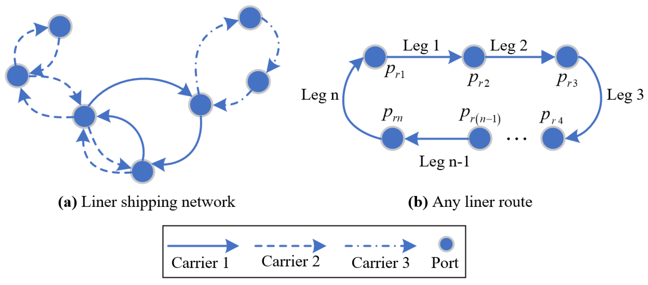
3.3. Liner Shipping Network Service

For describing our proposed problem, a liner shipping network operated by multiple cooperative liner carriers (namely a liner alliance) is considered. Furthermore, we provide a small liner shipping network as an example to describe the relationship between liner carriers and liner routes, as shown in Figure 1a. For our problem, we define any liner route $r$ as the calling sequence port, as shown in Figure 1b. In Figure 1b, $p_{r1}$ and $p_{rn}$ are the first port and the last port of liner route $r$. The voyage between $p_{ri}$ and $p_{r\left(i+1\right)}$ is leg $i$ of liner route $r$ ($\forall i\in I_r, \forall r\in R$).

This liner shipping network provides various container routes for ship containers to meet the container demand. We define $W_{od}^k$ as the set of alternative container routes for any OD pair $\left(o,d\right)$ from liner carrier $k$, which is fixed in advance. In addition, liner carriers deploy various types of ships to fulfill the weekly service frequency.

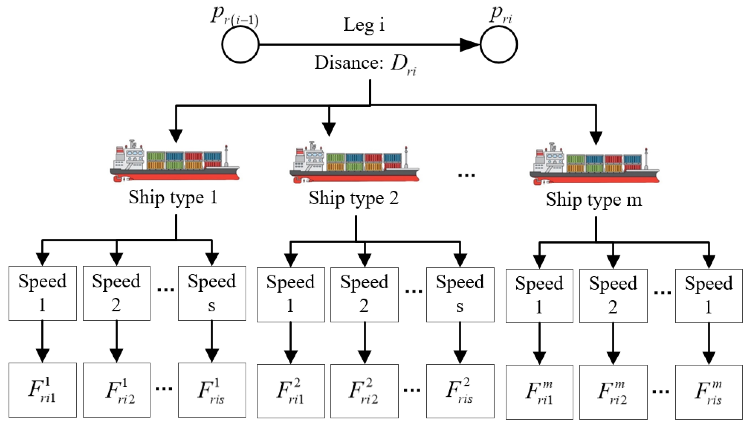
3.4. Cost and Time Structure

As mentioned before, in our considered liner shipping network, the cost structure includes the fixed cost of ship operations, the fuel costs and the cost of CEP trading.

For the cost associated with any liner route $r$, the fixed cost of ship operations is mainly dependent on ship types and ship numbers, which are decision variables in our proposed problem. The cost of CEP trading is determined by ship carbon emissions which are dependent on fuel consumption. The fuel costs are also dependent on fuel consumption. Following Fagerholt et al. [57] and Sun et al. [25], all possible fuel consumptions can be determined by

$$F_{ris}^m={\gamma }_m^{conversion}\times D_{ri}\times A_m{\left(s\right)}^{B_m-1}/24, \forall m\in M, \forall r\in R, \forall i\in I_r, \forall s\in S$$

(1)

$$s_{min}\le s\le s_{max}$$

(2)

$$F_{ri{s}_{min}}^m\le F_{ris}^m\le F_{ri{s}_{max}}^m, \forall m\in M, \forall r\in R, \forall i\in I_r, \forall s\in S$$

(3)

where $D_{ri}$ is the distance on leg $i$ of liner route $r$, $s_{min}$ and $s_{max}$ are the minimum and maximum sailing speeds, and $A_m{\left(s\right)}^{B_m-1}/24$ is the fuel consumption per nautical of ship type $m$ on leg $i$ of liner route $r$ with speed $s$. $A_m$ and $B_m$ are two parameters obtained by fitting actual data (Sun et al., 2022). Here, we provide a figure (namely Figure 2) to describe the relationship between alternative speed, alternative ship types and all possible fuel consumptions. Furthermore, ${\gamma }_m^{conversion}$ (${\gamma }_m^{conversion}\in \left(0,+\infty \right)$) is a conversion factor of fuels for ship type $m$ which aims to calculate LNG consumption based on oil consumption, and it can be obtained by the net calorific value of our considered fuels [48,51]. For VLSFO-powered ships, ${\gamma }_m^{conversion}$ is equal to 1. For LNG-powered ships, ${\gamma }_m^{conversion}$ can be determined by

$${\gamma }_m^{conversion}={\displaystyle \frac{Nc{v}_{LNG}}{Nc{v}_{VLSFO}}}, \forall m\in M_{LNG}$$

(4)

where $Nc{v}_{LNG}$ and $Nc{v}_{VLSFO}$ are the net calorific values of LNG and VLSFO.

For the time associated with any liner route $r$, the berthing time is mainly determined by the container shipment. All possible sailing times can be calculated by

$$T_{ris}^m=D_{ri}/s, \forall m\in M, \forall r\in R, \forall i\in I_r, \forall s\in S$$

(5)

$$T_{ri{s}_{max}}^m\le T_{ris}^m\le T_{ri{s}_{min}}^m, \forall m\in M, \forall r\in R, \forall i\in I_r, \forall s\in S$$

(6)

3.5. Allocation, Trading and Cap of Emission Permits

The process of the METS is described by adopting the METS planning period. For any planning period, the METS regulators allocate a number of free CEPs to liner carriers. For our considered cooperative liner carriers, the amount of free CEPs per week is calculated by the following:

$$E_{allocate}^k=\lambda \times E_{history}^k, \forall k\in K$$

(7)

where $\lambda$ is the free allocation factor of CEPs. $E_{history}^k$ is the historical carbon emissions from ships, which can be obtained from the ship data in the Automatic Identification System (AIS) or real ship scheduling data [39]. The usage of CEPs (or carbon emissions from ships) is limited by a cap, which is set by the METS regulators. Similarly to the free allocation of CEPs, the cap for our considered liner alliance can be described by

$$E_{alliance}^{cap}={\eta }^{cap}\times {\displaystyle \sum _{k\in K}{E}_{history}^k}$$

(8)

where ${\eta }^{cap}$ is a cap factor of the usage of CEPs.

3.6. Slot Co-Chartering Among Cooperative Liner Carriers

As an important mode of the cooperation of liner carriers, container slots can be co-chartered among cooperative liner carriers to provide a wider liner service. For leg $i$ of liner route $r$ ($\forall i\in I_r, \forall r\in R$), the balance between slot co-chartering in and slot co-chartering out needs to be ensured, described as follows:

$${\displaystyle \sum _{k\in K}{q}_{ri}^k}=0, \forall r\in R, \forall i\in I_r$$

(9)

where $q_{ri}^k$ is the amount of slots in leg $i$ of liner route $r$ co-chartered by carrier $m$ ($\forall i\in I_r, \forall r\in R, \forall k\in K$). $q_{ri}^k$ is a decision variable for our proposed problem. The positive value and the negative value of $q_{ri}^k$ represent slot chartering in and slot chartering out, respectively. For our considered liner alliances, container slot resources are integrated by slot co-chartering among cooperative liner carriers. Following Song and Wang [58], to describe the impact of liner alliances on the integration of slot resources more effectively, the balance between slot co-chartering in and slot co-chartering out is ensured, and the chartering of slots between liner carriers and container markets is not considered.

4. Model Development

4.1. Decision Variables

$q_{ri}^k$: Co-chartering volume of containers in leg $i$ of liner route $r$ for liner carrier $k$.

$x_{ris}^m$: Weight of the type $m$ ships on leg $i$ of liner route $r$ with speed alternative $s$.

$t_{ri}^{port}$: Time cost on the $i$-th port of liner route $r$.

$t_{ri}^{total}$: Total time of liner route $r$.

$y_w^k$: Container number transported on container liner route $w$ for liner carrier $k$.

$s{c}_r^k$: Auxiliary variable, number of container slots in liner route $r$ provided by liner carrier $k$.

$s{c}_r^{alliance}$: Auxiliary variable, the total slot number in liner route $r$ provided by the liner alliance.

$z_r^m$: Binary variable, takes value 1 if ships with type $m$ deployed on liner route $r$, or 0 otherwise.

$e_{trade}^k$: Traded volume of CEPs for liner carrier $k$.

$e_{usage}^k$: Usage of CEPs for liner carrier $k$.

$n_r^m$: Ship number of ship type $m$ deployed on liner route $r$.

$cos{t}_r^{VLSFO}$: Costs of deploying VLSFO-powered ships on liner route $r$.

$emissio{n}_r^{VLSFO}$: Carbon emissions of deploying VLSFO-powered ships on liner route $r$.

$cos{t}_r^{LNG}$: Costs of deploying LNG-powered ships on liner route $r$.

$emissio{n}_r^{LNG}$: Carbon emissions of deploying LNG-powered ships on liner route $r$.

4.2. Mathematical Model

Our proposed LFDP is formulated as the MILP:

$$\begin{array}{ll}\left[\mathrm{M}\mathrm{I}\mathrm{L}\mathrm{P}\right]& \begin{array}{l}min{\displaystyle \sum _{\left[\mathrm{MILP}\right] r\in R}{\displaystyle \sum _{m\in M}{C}_m^{fixed}\times n_r^m}}+{\displaystyle \sum _{k\in K}{c}^{permit}\times e_{trade}^k}\\ +{\displaystyle \sum _{m\in M}{\displaystyle \sum _{r\in R}{\displaystyle \sum _{i\in I_r}{\displaystyle \sum _{s\in S}{C}_m^{fuel}\times F_{ris}^m\times x_{ris}^m}}}}-{\displaystyle \sum _{k\in K}{\displaystyle \sum _{r\in R}{\displaystyle \sum _{i\in I_r}{P}_{k,ri}^{slot}\times q_{ri}^k}}}\end{array}\end{array}$$

(10)

which is subject to

(9);

$${\displaystyle \sum _{w\in W_{od}^k}{y}_w^k=Deman{d}_{od}^k}, \forall k\in K, \forall \left(o,d\right)\in P;$$

(11)

$${\omega }_r^k\times {\displaystyle \sum _{m\in M}{S}_m^{cap}\times z_r^m}=s{c}_r^k, \forall r\in R, \forall k\in K;$$

(12)

$${\displaystyle \sum _{m\in M}{S}_m^{cap}\times z_r^m}=s{c}_r^{alliance}, \forall r\in R;$$

(13)

$$-s{c}_r^k\le q_{ri}^k\le s{c}_r^{alliance}-s{c}_r^k, \forall k\in K, \forall r\in R, \forall i\in I_r$$

(14)

$${\displaystyle \sum _{w\in W_{od}^k}{\displaystyle \sum _{k\in K}\left(y_w^k\times {\pi }_{ri}^w\right)}}\le {\displaystyle \sum _{m\in M}{S}_m^{cap}}\times z_r^m, \forall r\in R, \forall i\in I_r;$$

(15)

$${\displaystyle \sum _{w\in W_{od}^k}{y}_w^k\times {\pi }_{ri}^w}\le {\omega }_r^k\times {\displaystyle \sum _{m\in M}{S}_m^{cap}\times z_r^m}+q_{ri}^k, \forall k\in K, \forall r\in R, \forall i\in I_r;$$

(16)

$$T^{handling}\times {\displaystyle \sum _{w\in W_{od}^k}{\displaystyle \sum _{k\in K}\left(y_w^k\times {\pi }_{ri}^w\right)}}\le t_{ri}^{port}, \forall r\in R, \forall i\in I_r;$$

(17)

$$t_{ri}^{port}+{\displaystyle \sum _{s\in S}{T}_{ris}^m\times x_{ris}^m}=t_{ri}^{total}, \forall r\in R, \forall i\in I_r;$$

(18)

$${\displaystyle \sum _{m\in M}{\displaystyle \sum _{r\in R}{\displaystyle \sum _{i\in I_r}{\displaystyle \sum _{s\in S}{\alpha }_m^{carbon}\times F_{ris}^m\times x_{ris}^m}}}}\le E_{alliance}^{cap};$$

(19)

$${\displaystyle \sum _{m\in M}{\displaystyle \sum _{r\in R}{\displaystyle \sum _{i\in I_r}{\displaystyle \sum _{s\in S}{\alpha }_m^{carbon}\times F_{ris}^m\times x_{ris}^m}}}}\times {\omega }_r^k=e_{usage}^k, \forall k\in K;$$

(20)

$${\displaystyle \sum _{s\in S}{x}_{ris}^m}=z_r^m, \forall m\in M, \forall r\in R, \forall i\in I_r;$$

(21)

$${\displaystyle \sum _{m\in M}{z}_r^m=1}, \forall r\in R;$$

(22)

$$z_r^m\le n_r^m\le \mathsf{\Omega }\times z_r^m, \forall m\in M, \forall r\in R;$$

(23)

$${\displaystyle \sum _{i\in I_r}{\displaystyle \sum _{s\in S}{T}_{ris}^m\times x_{ris}^m}}+{\displaystyle \sum _{i\in I_r}{t}_{ri}^{port}}\le 168\times n_r^m+\mathsf{\Omega }\times \left(1-z_r^m\right), \forall m\in M, \forall r\in R;$$

(24)

$$-E_{allocate}^k\le e_{usage}^k\le E_{allocate}^k+e_{trade}^k, \forall k\in K;$$

(25)

$$x_{ris}^m\in \left[0,1\right], \forall m\in M, \forall r\in R, \forall i\in I_r, \forall s\in S;$$

(26)

$$n_r^m\ge 0, \forall r\in R, \forall m\in M;$$

(27)

$$z_r^m\in \left\{0,1\right\}, \forall r\in R, \forall m\in M;$$

(28)

$$y_w^k\ge 0,\forall k\in K, \forall w\in W_{od}^k, \left(o,d\right)\in L;$$

(29)

$$t_{ri}^{port}\ge 0, \forall r\in R, \forall i\in I_r;$$

(30)

$$e_{usage}^k\ge 0, \forall k\in K;$$

(31)

$$cos{t}_r^{VLSFO}={\displaystyle \sum _{m\in M_{VLSFO}}{C}_m^{fixed}\times n_r^m}+{\displaystyle \sum _{m\in M_{VLSFO}}{\displaystyle \sum _{i\in I_r}{\displaystyle \sum _{s\in S}{C}_m^{fuel}\times F_{ris}^m\times x_{ris}^m}}}, \forall r\in R;$$

(32)

$$emissio{n}_r^{VLSFO}={\displaystyle \sum _{m\in M_{VLSFO}}{\displaystyle \sum _{i\in I_r}{\displaystyle \sum _{s\in S}{\alpha }_m^{carbon}\times F_{ris}^m\times x_{ris}^m}}}, \forall r\in R;$$

(33)

$$cos{t}_r^{LNG}={\displaystyle \sum _{m\in M_{LNG}}{C}_m^{fixed}\times n_r^m}+{\displaystyle \sum _{m\in M_{LNG}}{\displaystyle \sum _{i\in I_r}{\displaystyle \sum _{s\in S}{C}_m^{fuel}\times F_{ris}^m\times x_{ris}^m}}}, \forall r\in R;$$

(34)

$$emissio{n}_r^{LNG}={\displaystyle \sum _{m\in M_{LNG}}{\displaystyle \sum _{i\in I_r}{\displaystyle \sum _{s\in S}{\alpha }_m^{carbon}\times F_{ris}^m\times x_{ris}^m}}}, \forall r\in R.$$

(35)

The objective function (10) minimizes the total cost per week, and the profit of slot co-chartering is considered in our objective function to reflect the advantage of liner alliances. Constraints (11) denote that the demand of container shipment of liner carriers must be fulfilled. Constraints (12) and (13) determine the number of container slots provided in the liner route $r$. Constraints (14) denote the definition of the upper bound and lower bound of container slot co-chartering. Constraints (15) and (16) ensure that the number of containers transported via any leg of liner route $r$ is lower than the total number of container slots. Constraints (17) determine the berthing time dependent on the handled containers. Constraints (18) calculate the total time of liner route $r$. Constraints (19) ensure that carbon emissions are lower than the cap of CEPs determined by the METS regulators. Constraints (20) determine the usage of CEPs. Constraints (21) and (22) describe the relationship between ship deployment and ship sailing speeds. Constraints (23) limit the ship number. Constraints (24) ensure that the liner weekly service frequency must be fulfilled. Constraints (25) define the range of CEP trading. The decision variables of MILP are limited by Constraints (26)–(31). Constraints (32)–(35) determine the costs and carbon emissions of deploying VLSFO-powered ships and LNG-powered ships.

5. Numerical Experiments

5.1. Parameter Sets

In our numerical experiments, we consider a real Asia–Europe shipping network operated by multiple cooperative liner carriers.

Our considered liner shipping network consisting of 49 liner routes covers 46 ports, and this liner shipping network is operated by three cooperative carriers (denoted by Carrier 1, Carrier 2 and Carrier 3). In this liner shipping network, the large number of LNG bunkering stations can ensure the operations of LNG-powered ships (https://sea-lng.org/bunker-navigator/, accessed on 4 January 2025). Furthermore, for the countries and regions covered by this liner shipping network, the METS is considered and implemented to reduce ship carbon emissions [59] (https://www.eex.com/en/market-data/market-data-hub/environmentals/eex-eua-primary-auction-spot-download, https://eur-lex.europa.eu/legal-content/EN/TXT/?uri=CELEX%3A32023L0959&qid=1689499111676#d1e1638-134-1, accessed on 4 January 2025). Following Zheng et al. [55], we provide parameters including port calling sequences and container demands for this liner shipping network, which are shown in online Supplementary Materials. In addition, based on these ports and liner routes, 7385 container routes are given in advance for shipping containers.

The parameters of all alternative types of ships are shown in

Table 3. Parameters of all alternative types of ships.

Ship Type  $\mathit{m}$	1	2	3	4
Capacity (TEU)	3000	8000	12,000	18,000
Powered by	Fuel	Fuel	Fuel	Fuel
$A_m$	0.012	0.0108	0.013	0.015
$B_m$	2.815	3.026	3.207	3.371
${\gamma }_m^{conversion}$	1	1	1	1
Fixed cost (USD 103 )	70.9	142.7	216.8	285.8
Ship Type  $\mathit{m}$	5	6	7	8
Capacity (TEU)	3000	8000	12,000	18,000
Powered by	LNG	LNG	LNG	LNG
$A_m$	0.012	0.0108	0.013	0.015
$B_m$	2.815	3.026	3.207	3.371
${\gamma }_m^{conversion}$	0.84	0.84	0.84	0.84
Fixed cost (USD 103)	85.08	171.24	260.16	342.96

[16,39,48]. In addition, a virtual ship type is considered, with a capacity, operating cost and fuel consumption of zero. If a virtual ship is deployed, it means that the liner route can be discontinued.

The parameters of VLSFO and LNG are shown in Table 1, including carbon emission factors and net calorific values. For fuel prices, the prices of VLFSO and LNG are set as 500 USD/ton and 600 USD/ton, which follow the Clarksons data (https://www.clarksons.net/n/#/sin/timeseries/browse;e=%5B40882%5D;c=%5B51431%5D/(ts:data/100/latest;t=%5B548864,548868,548872%5D;l=%5B548864,548868,548872%5D;exportAsPNG=false;listMode=false;viewMode=ChartAndGrid), accessed on 4 January 2025). More results with various fuel prices are provided in Section 5.4. $v_{max}$ is set as 20 knots, and $v_{min}$ is set as 8 knots.

For cooperative liner carriers, the details of slot co-chartering are usually considered trade secrets. Hence, in this paper, we set $p_{m,ri}^{slot}$ by multiplying a random rate (within the range of 0 to 0.3) of profit by the actual container freight (https://www.yqn.com/). Following the METS regulations (https://eur-lex.europa.eu/legal-content/EN/TXT/?uri=CELEX%3A32023L0959&qid=1689499111676#d1e1638-134-1, accessed on 4 January 2025) in practice, the free allocation rate of CEPs is set as 0.5, and ${\eta }^{cap}$ is 0.9. More results with different free allocation rates and trading prices of CEPs are provided in Section 5.3. Following Sun et al. [39], based on the ship scheduling, we can obtain the historical carbon emissions per week produced by our considered liner carriers, namely $e_{history}^1=15787.1$, $e_{history}^2=50919$ and $e_{history}^3=52218$.

To program our models, we employ Visual C++ (2022) on a PC equipped with a 2.9 GHz Quad Core processor. Moreover, utilizing CPLEX 12.6, we can solve our models efficiently.

5.2. Comparison Analysis

In this subsection, we compare the total cost from the perspective of a liner alliance and a single carrier. For any single liner carrier, the total cost can be obtained by a new model (called SMILP), which can be obtained by simplifying our proposed MOPSO. Note that, for our SMILP, the index $k$ ($\forall k\in K$) in notations, parameters and decision variables can be ignored. The SMILP can be developed as follows:

$$\left[\mathrm{SMILP}\right] min{\displaystyle \sum _{r\in R}{\displaystyle \sum _{m\in M}{C}_m^{fixed}\times n_r^m}}+{\displaystyle \sum _{k\in K}{c}^{permit}\times e_{trade}^k}+{\displaystyle \sum _{m\in M}{\displaystyle \sum _{r\in R}{\displaystyle \sum _{i\in I_r}{\displaystyle \sum _{s\in S}{C}_m^{fuel}\times F_{ris}^m\times x_{ris}^m}}}}$$

(36)

(19), (21)–(23), (26)–(28), (30), (31);

Subject to

$${\displaystyle \sum _{h\in W_{od}}{y}_h=Deman{d}_{od}}, \forall \left(o,d\right)\in L;$$

(37)

$$T^{handling}\times {\displaystyle \sum _{h\in W_{od}}\left(y_h\times {\delta }_{ri}^h\right)}\le t_{ri}^{port}, \forall r\in R, \forall i\in I_r;$$

(38)

$${\displaystyle \sum _{h\in W_{od}}\left(y_h\times {\delta }_{ri}^h\right)}\le {\displaystyle \sum _{k\in K}{S}_k^{cap}}\times z_r^k, \forall r\in R, \forall i\in I_r;$$

(39)

$${\displaystyle \sum _{i\in I_r}{\displaystyle \sum _{s\in S}{T}_{ris}^m\times x_{ris}^m}}+{\displaystyle \sum _{i\in I_r}{t}_{ri}^{port}}\le 168\times n_r^m+\mathsf{\Omega }\times \left(1-z_r^m\right), \forall m\in M, \forall r\in R;$$

(40)

$${\displaystyle \sum _{m\in M}{\displaystyle \sum _{r\in R}{\displaystyle \sum _{i\in I_r}{\displaystyle \sum _{s\in S}{\alpha }_m^{carbon}\times F_{ris}^m\times x_{ris}^m}}}}\le E_{alliance}^{cap};$$

(41)

$$-E_{allocate}\le e_{trade};$$

(42)

$$y_h\ge 0, \forall h\in W_{od}, \left(o,d\right)\in L.$$

(43)

A cost comparison between the liner alliance and single liner carrier is shown in

Table 4. Cost comparison between the liner alliance and single liner carrier (USD 10⁶).

Trading Price of CEPs (USD/tons)	Liner Alliance	Single Liner Carrier				Cost Reduction Rate (%)
		Carrier 1	Carrier 2	Carrier 3	Sum
0	55.36	5.93	28.86	23.13	57.92	3.54%
30	56.46	6.00	29.16	23.37	58.53	3.00%
60	57.26	6.05	29.41	23.57	59.03	2.51%
90	57.82	6.08	29.55	23.68	59.31	1.84%
120	58.30	6.09	29.59	23.71	59.39	3.86%
150	58.58	6.08	30.56	24.29	60.93	4.57%
180	58.83	6.06	30.97	24.62	61.65	5.89%
210	58.97	6.04	31.38	25.24	62.66	7.43%
240	59.05	6.00	32.01	25.78	63.79	9.14%
270	59.02	5.94	32.88	26.14	64.96	10.79%
300	58.80	5.87	33.15	26.89	65.91	11.43%
330	58.52	5.80	33.98	26.29	66.07	3.54%

. Similarly to the liner alliance, for any single liner carrier, the total cost shows a tendency to increase and then decrease with the increase in CEP trading price. However, the total cost of liner carriers without considering cooperation is higher than the cost of forming liner alliances.

5.3. Results with Different CEP Trading Prices

In this subsection, we mainly show the results of fleet deployment, ship speeds and the trading of CEPs with various trading prices of CEPs.

First, we show fleet deployment in various liner routes with various CEP trading prices. To simplify, we adopt the ship capacity with the expected ship type ($S_r^{deploy}$) to describe the choice of ship types. Let $p_r^k$ denote the frequency of deploying ship type $k$ on liner route $r$ in all solutions with various CEP trading prices (from 0 to 330 USD/ton) ($\forall r\in R, \forall k\in K$). Then, $S_r^{deploy}$ can be obtained by

$$S_r^{deploy}=⌈{\displaystyle \sum _{m\in M}{S}_m^{cap}\times p_r^m}⌉, \forall r\in R$$

(44)

Figure 3a–c show the ship capacity of various liner routes for Carrier 1, Carrier 2 and Carrier 3, respectively. In Figure 3, we can find that most liner routes deploy small ships, and several liner routes (e.g., 11, 12, 34 and 37) deploy large and mega ships. In addition, the shipping service of several liner routes (e.g., Route 19, 21, 22, 24, 29, 32 and 38) can be discontinued, and no ships are deployed in these liner routes. According to online Supplementary Materials, we can find that discontinued liner routes are mainly feeder liner routes. The discontinuation of liner routes is mainly due to the transfer of containers through slot co-chartering, and containers transfer trunk liner routes from feeder liner routes. We provide the results on carbon emission of our considered liner routes with various CEP trading prices in Appendix A, where carbon emission can reflect the deployment of ships effectively. From Appendix A, we can obtain that the impact of CEP trading prices and fuel prices on the discontinuation of liner routes can be ignored. This is because, in our proposed MILP model, CEP trading prices and fuel prices mainly determine ship speeds, the deployed number of ships and CEP trading, rather than slot co-chartering and container shipment, which are limited by the provided alternative container routes from liner carriers in advance.

Figure 4 shows the number of ships with various CEP trading prices. Figure 4 shows that 3000-TEU ships are the most deployed, followed by 8000-TEU ships and 18,000-TEU ships, and 12,000-TEU ships are the least deployed. As the CEP trading price increases, the number of ships has an obvious increase. In addition, compared with other ship types, the deployed number of 3000-TEU ships is more sensitive to the trading price of CEPs.

In Figure 5, we show the deployment frequency of LNG-powered ships with various CEP trading prices. When the trading price of CEPs is low (e.g., 0 to 125 USD/ton), due to the large operational cost of LNG-powered ships, liner carriers prefer to deploy VLSFO-powered ships. For liner carriers, the additional cost of buying CEPs is less than that of deployed LNG-powered ships. When the trading price of CEPs is medium (e.g., 125 to 250 USD/ton), 3000-TEU ships are the first to adopt LNG in response to the increasing CEP trading prices. When the trading price of CEPs is high (e.g., 250 to 330 USD/ton), all VLSFO-powered ships are gradually replaced with LNG-powered ships. For liner carriers, deploying LNG-powered ships can save a number of CEPs, and selling the surplus CEP can reduce the total cost. In addition, we can find that LNG is adopted in 3000-TEU ships and 18,000-TEU ships completely, which have the maximum deployed number and the maximum fixed cost, respectively.

We show the deceleration rate of ships for various liner routes in

Table 5. Deceleration rate of ships for various liner routes.

Route	Rate	Route	Rate	Route	Rate
1	37.89%	15	18.54%	35	18.05%
2	21.45%	16	24.31%	36	23.37%
3	0.00%	17	17.86%	37	15.70%
4	0.00%	18	10.28%	39	19.19%
5	17.07%	20	17.91%	40	16.70%
6	0.00%	23	21.72%	41	18.22%
7	44.37%	25	0.11%	42	17.01%
8	21.57%	26	16.60%	43	21.63%
9	19.60%	27	0.00%	44	0.11%
10	0.00%	28	0.00%	45	20.57%
11	18.08%	30	0.00%	46	17.27%
12	17.26%	31	20.95%	47	16.52%
13	17.98%	33	0.00%	48	0.00%
14	18.36%	34	18.35%	49	0.00%

when the CEP trading price increases from 0 to 330 (USD/ton). Note that we have deleted the results of several liner routes which can be discontinued from Table 3. We can find that the ship speeds on most liner routes decrease significantly, with the increase in CEP trading price. Note that the deceleration rates of several liner routes are 0. This is because, when the trading price of CEP is 0, the ship speed of these liner routes is the minimum speed.

We show the results of carbon emissions for various ship types in Figure 6. The highest carbon emissions are from 18,000-TEU ships, followed by 3000-TEU and 8000-TEU ships, and the lowest emissions are from 12,000-TEU ships. We can find a two-stage reduction in ship carbon emissions for any ship type. Combined with Figure 4, the first stage of the reduction in carbon emissions is mainly generated by ship deceleration, while the second stage is mainly due to the deployment of LNG-powered ships.

Table 6. Total costs, carbon emissions and traded CEPs with various CEP trading prices.

Trading Price of CEPs (USD/ton)	Total Cost (USD 106)	Carbon Emissions (tons)	Traded CEPs (tons)
			Carrier 1	Carrier 2	Carrier 3
0	55.36	97,789.52	9259	12,597	16,453
30	56.46	94,925.76	8246.11	11,877.63	15,319.97
60	57.26	79,898.41	3935.41	7984.15	8496.81
90	57.82	77,182.47	3776.58	6877.85	7045.98
120	58.30	69,936.91	3717.19	3752.64	2985.01
150	58.58	68,042.45	3249.59	2994.25	2316.56
180	58.83	67,442.03	3249.59	2748.78	1961.61
210	58.97	62,684.05	2677.83	−877.43	1401.6
240	59.05	60,692.84	2677.83	−1639.48	172.44
270	59.02	53,893.86	691.4	−3880.55	−2399.04
300	58.80	51,620.82	477.5	−4018.19	−4320.53
330	58.52	48,679.92	52.14	−4727.35	−6126.92

shows the total cost, carbon emissions and the trading of CEPs of our considered liner alliance with various trading prices of CEPs. For the traded CEPs, a positive value means the buying of CEPs, and a negative value means the selling of CEPs. For the liner alliance, the total cost shows a tendency to increase and then decrease as the CEP trading prices increase. The trading of CEPs brings more additional costs for the liner alliance. When the trading price of CEPs is high, the liner alliance (or liner carrier) prefers to deploy LNG-powered ships and sell CEPs to reduce the total cost. The trading of CEPs of cooperative liner carriers also supports this phenomenon.

Next, we provide the results on the costs and carbon emissions of operating LNG-powered and VLSFO-powered ships with various trading prices of CEPs, as shown in

Table 7. Costs and carbon emissions of ship deployment with various CEP trading prices.

CEP Price (USD/ton)	VLSFO-Powered Ships		LNG-Powered Ships		Sum
	Cost (USD 106)	Carbon Emissions (103 tons)	Cost (USD 106)	Carbon Emissions (103 tons)	Cost (USD 106)	Carbon Emissions (103 tons)
30	55.40	94.93	0.00	0.00	55.40	94.93
60	55.84	79.60	0.14	0.30	55.97	79.90
90	56.23	77.18	0.00	0.00	56.23	77.18
120	56.95	69.78	0.10	0.15	57.05	69.94
150	56.05	66.49	1.18	1.56	57.23	68.04
180	55.75	65.37	1.65	2.07	57.39	67.44
210	54.28	58.40	3.95	4.29	58.24	62.68
240	48.80	51.08	9.96	9.62	58.76	60.69
270	28.10	27.16	32.43	26.74	60.53	53.89
300	21.52	19.99	39.57	31.63	61.09	51.62
330	11.23	9.92	50.86	38.76	62.09	48.68

. In Table 7, we can find that (i) as the CEP trading price increases, the costs of deploying VLSFO-powered ships decrease, and the costs of deploying LNG-powered ships rise; (ii) compared with the total cost shown in Table 6, when the trading price is high, the deployed LNG-powered ships decrease their sailing speed to save more CEPs, and selling these surplus CEPs can reduce the costs of deploying LNG-powered ships.

Finally, as shown in Figure 7, we compare carbon emissions and total costs under various allocations of CEPs, which are dependent on parameter $\lambda$. In Figure 7a, we can find that the carbon emissions under various CEP allocations are nearly the same, and all of them decrease as the CEP price increases. In Figure 7b, we can find that the total costs of the liner alliance under various CEP allocations are different. The larger the value of $\lambda$, the lower the total cost of the liner alliance. Comparing Figure 7a and Figure 7b, the total cost is sensitive to the allocation and trading price of CEPs, while carbon emissions are sensitive only to the trading price of CEPs.

5.4. Results with Different Fuel Prices

In this subsection, we mainly analyze the impact of fuel prices (including VLSFO prices and LNG prices) on the total cost, carbon emissions and ship deployments, as shown in Figure 8, Figure 9 and

Table 8. Costs and carbon emissions of ship deployment with various LNG prices.

LNG Price (USD/ton)	VLSFO-Powered Ships		LNG-Powered Ships		Total
	Cost (USD 106)	Carbon Emissions (103 tons)	Cost (USD 106)	Carbon Emissions (103 tons)	Cost (USD 106)	Carbon Emissions (103 tons)
100	0.49	0.30	40.94	106.40	41.43	106.7
200	0.49	0.35	44.32	106.36	44.81	106.71
300	0.70	0.51	48.55	99.94	49.25	100.45
400	45.88	81.29	6.70	10.37	52.58	91.66
500	52.43	94.93	/	/	52.43	94.93
600	52.43	94.93	/	/	52.43	94.93
700	52.43	94.93	/	/	52.43	94.93
800	52.43	94.93	/	/	52.43	94.93
900	52.43	94.93	/	/	52.43	94.93

.

We analyze the impact of fuel prices on carbon emissions. Figure 8 shows carbon emissions from ships with various fuel prices. We witness the following phenomena: (i) carbon emissions from ships show a significant reduction as the fuel price increases; (ii) when the VLSFO price is low, the change in LNG prices has almost no effect on ship carbon emissions; (iii) when the LNG price is high, there is a significant effect of the change in VLSFO price on the carbon emissions from ships.

Next, we mainly analyze the impact of LNG prices on the results. The VLSFO price is set as 400 USD/ton, and the trading price of CEPs is set as 60 USD/ton. Figure 9 shows the number of deployed LNG-powered ships with various LNG prices. In Figure 9, we can find that, as the LNG price increases, the number of deployed LNG-powered ships gradually decreases, and liner carriers gradually begin to deploy VLSFO-powered ships. When the LNG price is more than 500 USD/ton, liner carriers prefer to deploy VLSFO-powered ships completely, rather than LNG-powered ships.

Furthermore, in Table 8, we provide the results on the costs and carbon emissions of deploying LNG-powered and VLSFO-powered ships with various LNG prices, respectively. In Table 8, we can also find that, as the LNG price increases, liner carriers gradually replace LNG-powered ships with VLSFO-powered ships, and the costs and carbon emissions of deploying LNG-powered ships are also transferred. Note that, when the VLSFO price and the LNG price are similar (400 USD/ton), we can obtain a solution with the lowest carbon emissions. This is because, when the LNG price is low, liner carriers increase ship speeds and produce more carbon emissions, and liner carriers deploy VLSFO-powered ships (which have a higher emission factor) completely when the LNG price is high.

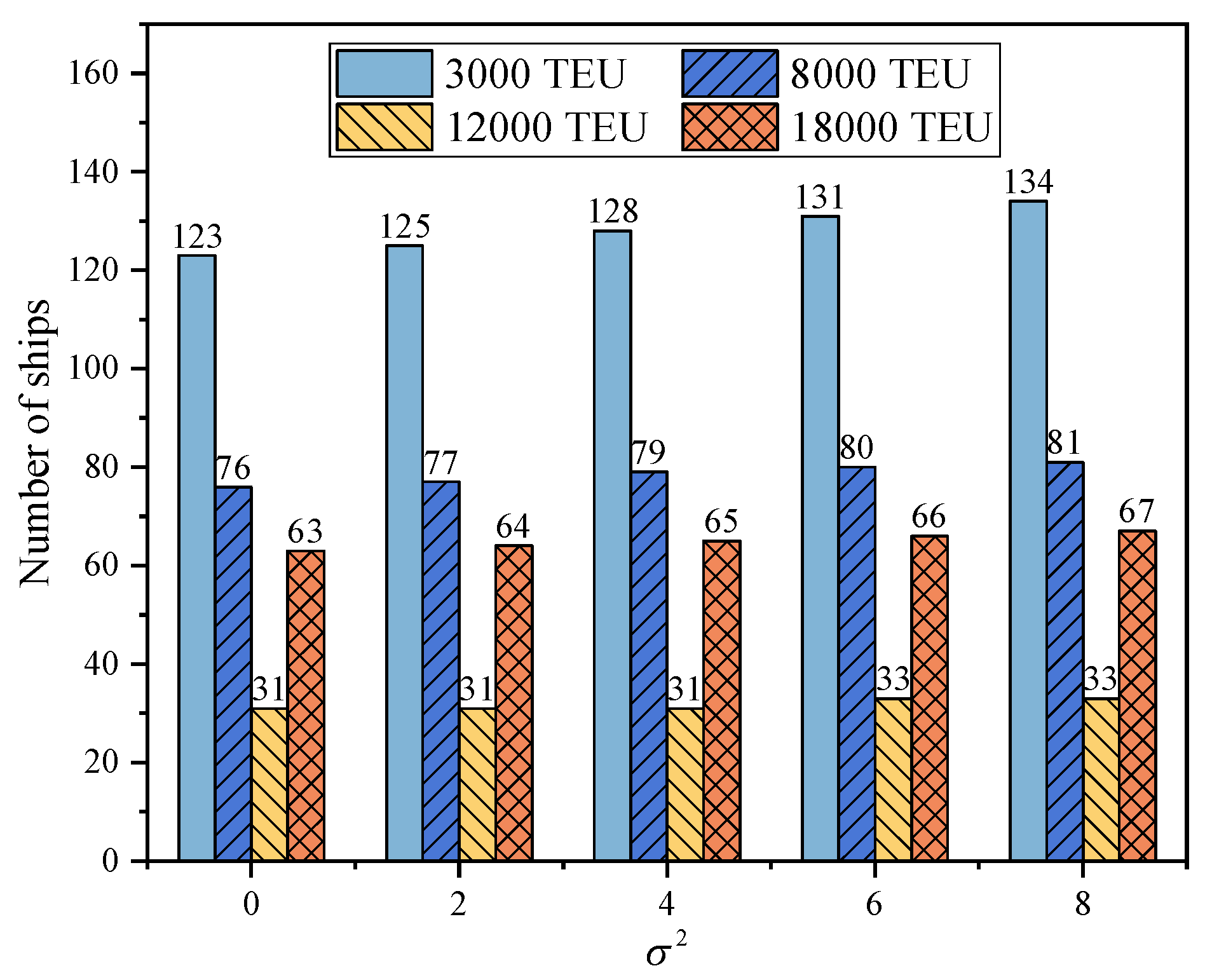
5.5. Expanded Results Considering Uncertain Navigational Risks

In this subsection, we provide expanded results considering uncertain navigational risks (e.g., bad weather, port disruptions and port congestions), which lead to longer sailing times and port times. To describe the impact of these uncertain navigational risks, we introduce the delay time in the leg $i$ of the liner route $r$($t_{ri}^{delay}$), which is a decision variable and is dependent on chance constraints. Considering the uncertain delay time, our MILP model can be expanded as the following model (named UMIP):

$$\begin{array}{ll}\left[\mathrm{U}\mathrm{M}\mathrm{I}\mathrm{P}\right]& \begin{array}{l}min{\displaystyle \sum _{r\in R}{\displaystyle \sum _{m\in M}{C}_m^{fixed}\times n_r^m}}+{\displaystyle \sum _{k\in K}{c}^{permit}\times e_{trade}^k}+{\displaystyle \sum _{m\in M}{\displaystyle \sum _{r\in R}{\displaystyle \sum _{i\in I_r}{\displaystyle \sum _{s\in S}{C}_m^{fuel}\times F_{ris}^m\times x_{ris}^m}}}}\\ +{\displaystyle \sum _{r\in R}{\displaystyle \sum _{i\in I_r}{C}^{penalty}\times \left(T_{ri}^{scheduling}-t_{ri}^{total}\right)}}-{\displaystyle \sum _{k\in K}{\displaystyle \sum _{r\in R}{\displaystyle \sum _{i\in I_r}{P}_{k,ri}^{slot}\times q_{ri}^k}}}\end{array}\end{array}$$

(45)

which is subject to

(9), (11)–(17), (19)–(23), (25)–(31);

$${\displaystyle \sum _{i\in I_r}{\displaystyle \sum _{s\in S}{T}_{ris}^m\times x_{ris}^m}}+{\displaystyle \sum _{i\in I_r}{t}_{ri}^{port}+t_{ri}^{delay}}\le 168\times n_r^m+\mathsf{\Omega }\times \left(1-z_r^m\right), \forall m\in M, \forall r\in R;$$

(46)

$$t_{ri}^{delay}+t_{ri}^{port}+{\displaystyle \sum _{s\in S}{T}_{ris}^m\times x_{ris}^m}=t_{ri}^{total}, \forall r\in R, \forall i\in I_r;$$

(47)

$$Pr\left({\tilde{t}}_{ri}^{delay}\le t_{ri}^{delay}\right)\ge {\phi }^{delay}, \forall r\in R, \forall i\in I_r;$$

(48)

$$t_{ri}^{delay}\ge 0, \forall r\in R, \forall i\in I_r.$$

(49)

where $T_{ri}^{scheduling}$ is the planning time in the leg $i$ of the liner route $r$ and is obtained from the actual ship scheduling of liner carriers. $C^{penalty}$ is the penalty cost of the delay per hour. Constraints (46) are chance constraints adopted to describe the uncertainty in the delay time of liner routes, where ${\phi }^{delay}$ is the confidence level for the delay time distribution.

To solve our UMIP, we rewrite chance constraints (48) as deterministic constraints. For our considered liner shipping network, we assume that the delay time follows a normal distribution. We define ${\varsigma }^{-1}\left(\cdot \right)$ as the inverse function of the distribution of the delay time. Then, chance constraints (46) can be transformed as

$$t_{ri}^{delay}\ge {\varsigma }_{{\tilde{t}}_{ri}^{delay}}\left({\phi }^{delay}\right), \forall r\in R, \forall i\in I_r$$

(50)

In this subsection, we define $N\left(\mu , {\sigma }^2\right)$ as the distribution function of the delay time. $\mu$ is the mean value of delay times, and it can be obtained by AIS data. Following Zhen and Chang [60] and Guo et al. [61], we develop a scenario generator to simulate various scenarios, and we define ${\sigma }^2$ as the degree of uncertainty. For other parameters, $T_{ri}^{scheduling}$ can be generated by following Wang and Meng [62]. For liner shipping, we aim to avoid the delay by setting $C^{penalty}$ as an infinite number. ${\phi }^{delay}$ is set as 0.95. For our results, we mainly consider ${\sigma }^2=0,2,4,6,8$.

In

Table 9. Costs and emissions of ship deployment with various LNG prices.

${\mathit{\sigma }}^2$	Total Cost (USD 106)	Carbon Emissions (103 tons)	Ship Power
0	54.56	94.93	VLSFO
2	55.19	95.52	VLSFO
4	56.01	96.15	VLSFO
6	56.59	93.70	VLSFO
8	57.36	94.40	VLSFO

, we provide the total cost, carbon emissions and ship power as the value of ${\sigma }^2$ increases; we can find that the total cost rises, while carbon emissions are unstable and the deployed ships are powered by VLSFO. The choice of ship powers is not dependent on the uncertain delay time of liner routes. Furthermore, we show the number of deployed ships with various ${\sigma }^2$ in Figure 10. We can also find that, with the increase in ${\sigma }^2$, there is a significant increase in the number of deployed ships. This means liner carriers have to deploy more ships to deal with uncertain delay times.

6. Conclusions

From the perspective of liner alliances, this paper investigates the deployment of LNG-powered ships in response to the METS. We propose an LFDP combined with slot co-chartering and CEP trading, and develop an MILP model. Based on the results of our proposed problem and model, the following conclusions are drawn:

(i)

Compared with the results without considering the cooperation of liner carriers, the formation of liner alliances reduces the total cost of cooperative liner carriers, which consider the deployment of LNG-powered ships in response to the METS. To reduce the additional cost of CEP trading and deploying LNG-powered ships, shipping carriers can form a coalition to participate in the allocation and trading of CEPs for accelerating the deployment of LNG-powered ships. For our numerical experiments, the cooperation of liner carriers can reduce the total cost by about 3~11% with various CEP trading prices.

(ii)

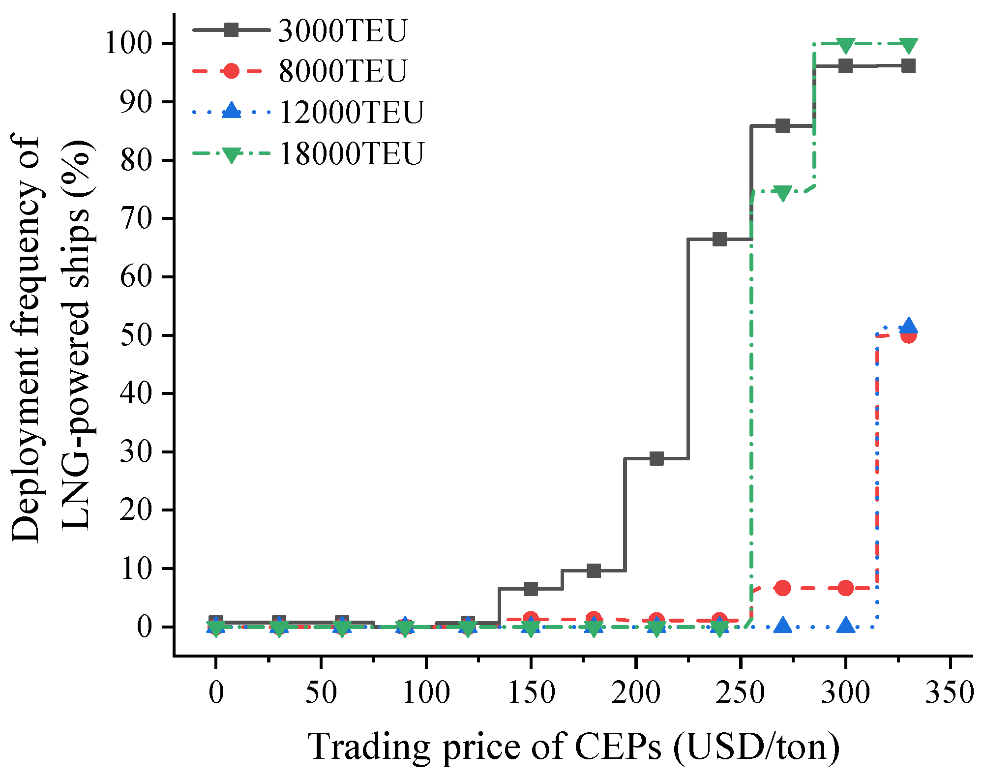
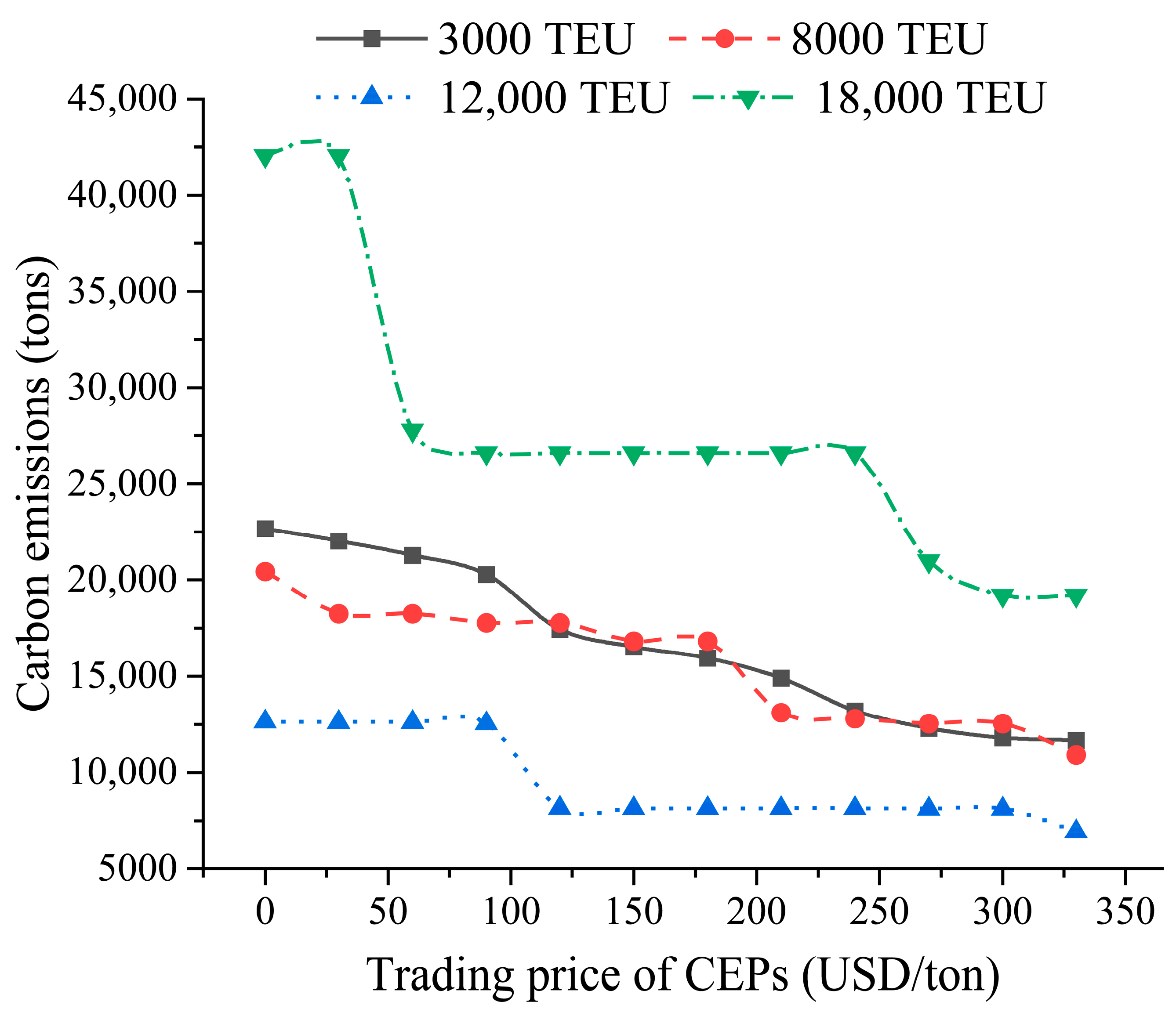
The trading price of CEPs determines the total cost and ship carbon emissions of liner alliances. When the trading price of CEPs is low, it is economical for cooperative liner carriers to adopt the slow-down strategy to reduce carbon emissions from VLSFO-powered ships. The low trading price of CEPs (e.g., less than 150 USD/ton) hardly encourages shipping carriers to deploy LNG-powered ships. For accelerating the deployment of LNG-powered ships, METS regulators can raise the CEP trading price above 150 USD/ton through regulatory adjustments.

(iii)

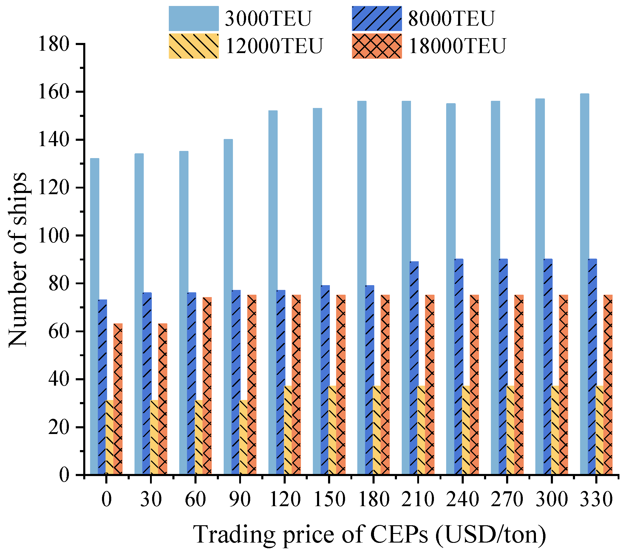
When the CEP trading price is high (more than 150 USD/ton), shipping carriers should deploy small LNG-powered ships (e.g., 3000-TEU) first to reduce carbon emissions and the additional cost of trading CEPs. Then, as the CEP trading price increases, shipping carriers should complete the fuel conversion from VLSFO to LNG for small LNG-powered ships and mega LNG-powered ships (e.g., 18,000-TEU), which have the maximum deployed number and the maximum fixed cost.

Our research still has some limitations that will be addressed in the future.

(i)

The allocation and trading of CEPs encourage shipping carriers to invest in green shipping technologies including the reconstruction of LNG-powered ships. However, the economic interaction between CEP trading and the reconstruction cost of LNG-powered ships is not assessed in this paper. In future work, we will analyze the impact of CEP trading on the reconstruction of LNG-powered ships.

(ii)

Sulphur emission regulations (e.g., ECAs and the global sulphur limit) bring more operation costs for oil-powered ships, and these regulations also encourage shipping carriers to adopt LNG-powered ships, which produce virtually no sulphur emissions. In future work, we will investigate the deployment of LNG-powered ships in response to various sulphur emission regulations, as well as regulations pertaining to both sulphur and carbon emission reductions.

References

1. UNCTAD. Review of Maritime Transportation 2022; Paper Presented at the United Nations Conference on Trade and Development; UNCTAD: New York, NY, USA; Geneva, Switzerland, 2023. [Google Scholar]
2. Gu, Y.; Wallace, S.; Wang, X. Can an Emission Trading Scheme really reduce CO2 emissions in the short term? Evidence from a maritime fleet composition and deployment model. Transp. Res. Part D Transp. Environ. 2019, 74, 318–338. [Google Scholar] [CrossRef]
3. Davies, M. Emissions trading for ships—A European perspective. Nav. Eng. J. 2006, 118, 131–138. [Google Scholar] [CrossRef]
4. Kågeson, P. Linking CO2 Emissions from International Shipping to the EU ETS. 2007. Available online: http://www.natureassociates.se/wp-content/uploads/2011/03/Linking-CO2-Emissions-from-International-Shipping-to-the-EU-ETS.pdf (accessed on 15 February 2018).
5. Schinas, O.; Bergmann, N. Emissions trading in the aviation and maritime sector: Findings from a revised taxonomy. Clean. Logist. Supply Chain. 2021, 1, 100003. [Google Scholar] [CrossRef]
6. Ye, J.; Chen, J.; Shi, J.; Jiang, X.; Zhou, S. Novel synergy mechanism for carbon emissions abatement in shipping decarbonization. Transp. Res. Part D Transp. Environ. 2024, 127, 104059. [Google Scholar] [CrossRef]
7. Christodoulou, A.; Dalaklis, D.; Olcer, A.; Masodzadeh, P. Inclusion of Shipping in the EU-ETS: Assessing the direct costs for the maritime sector using the MRV data. Energies 2021, 14, 3915. [Google Scholar] [CrossRef]
8. Wang, T.; Cheng, P.; Wang, Y. How the establishment of carbon emission trading system affects ship emission reduction strategies designed for sulfur emission control area. Transp. Policy 2025, 160, 138–153. [Google Scholar] [CrossRef]
9. Kim, J.; Kim, H.; Lee, P. Optimizing containership speed and fleet size under a carbon tax and an emission trading scheme. Int. J. Shipp. Transp. Logist. 2013, 5, 571–590. [Google Scholar] [CrossRef]
10. Haehl, C.; Spinler, S. Technology choice under emission regulation uncertainty in international container shipping. Eur. J. Oper. Res. 2019, 284, 383–396. [Google Scholar] [CrossRef]
11. Kenan, N.; Jebali, A.; Diabat, A. The integrated quay crane assignment and scheduling problems with carbon emissions considerations. Comput. Ind. Eng. 2022, 165, 107734. [Google Scholar] [CrossRef]
12. Xue, Y.; Lai, K.; Wang, C. How to invest decarbonization technology in shipping operations? Evidence from a game-theoretic investigation. Ocean Coast. Manag. 2024, 251, 107076. [Google Scholar] [CrossRef]
13. Wang, T.; Cheng, P.; Zhen, L. Green development of the maritime industry: Overview, perspectives, and future research opportunities. Transp. Res. Part E Logist. Transp. Rev. 2023, 179, 138–153. [Google Scholar] [CrossRef]
14. Wu, Y.; Wang, S.; Chen, Y.; Chang, D. Evaluation of liquefied natural gas as a ship fuel for liner shipping using evolutionary game theory. Asia-Pac. J. Oper. Res. 2021, 38, 2140022. [Google Scholar] [CrossRef]
15. Li, D.; Yang, H.; Xing, Y. Economic and emission assessment of LNG-fuelled ships for inland waterway transportation. Ocean Coast. Manag. 2023, 246, 106906. [Google Scholar] [CrossRef]
16. Qi, J.; Wang, H.; Zheng, J. Promoting liquefied natural gas (LNG) bunkering for maritime transportation: Should ports or ships be subsidized? Sustainability 2022, 14, 6928. [Google Scholar] [CrossRef]
17. Zhao, Z.; Wang, X.; Wang, H.; Cheng, S.; Liu, W. Fleet deployment optimization for LNG shipping vessels considering the influence of mixed factors. J. Mar. Sci. Eng. 2022, 10, 2034. [Google Scholar] [CrossRef]
18. Yuan, J.; Shi, X.; He, J. LNG market liberalization and LNG transportation: Evaluation based on fleet size and composition model. Appl. Energy 2024, 358, 122657. [Google Scholar] [CrossRef]
19. Shih, Y.C.; Tzeng, Y.; Cheng, C.; Huang, C. Speed and fuel ratio optimization for a dual-fuel ship to minimize its carbon emissions and cost. J. Mar. Sci. Eng. 2023, 11, 758. [Google Scholar] [CrossRef]
20. He, P.; Jin, J.; Pan, W.; Chen, J. Route, speed, and bunkering optimization for LNG-fueled tramp ship with alternative bunkering ports. Ocean Eng. 2024, 305, 117957. [Google Scholar] [CrossRef]
21. Sun, L.; Wang, X.; Hu, Z.; Liu, W.; Ning, Z. Carbon reduction and cost control of container shipping in response to the European Union Emission Trading System. Environ. Sci. Pollut. Res. 2024, 31, 21172–21188. [Google Scholar] [CrossRef]
22. Christiansen, M.; Fagerholt, K.; Ronen, D. Ship routing and scheduling: Status and perspectives. Transp. Sci. 2004, 38, 1–120. [Google Scholar] [CrossRef]
23. Dulebenets, M.; Pasha, J.; Abioye, O.; Kavoosi, M. Vessel scheduling in liner shipping: A critical literature review and future research needs. Flex. Serv. Manuf. J. 2019, 33, 43–106. [Google Scholar] [CrossRef]
24. Chen, J.; Ye, J.; Zhuang, C.; Qin, Q.; Shu, Y. Liner shipping alliance management: Overview and future research directions. Ocean. Coast. Manag. 2022, 219, 106039. [Google Scholar] [CrossRef]
25. Sun, Y.; Zheng, J.; Yang, L.; Li, X. Allocation and trading schemes of the maritime emissions trading system: Liner shipping route choice and carbon emissions. Transp. Policy 2024, 148, 60–78. [Google Scholar] [CrossRef]
26. Haites, E. Linking emissions trading schemes for international aviation and shipping emissions. Clim. Policy 2009, 9, 415–430. [Google Scholar] [CrossRef]
27. Schinas, O.; Butler, M. Feasibility and commercial considerations of LNG-fueled ships. Ocean Eng. 2016, 122, 84–96. [Google Scholar] [CrossRef]
28. Jeong, H.; Yun, H. A stochastic approach for economic valuation of alternative fuels: The case of container ship investments. J. Clean. Prod. 2023, 418, 138182. [Google Scholar] [CrossRef]
29. Xu, H.; Yang, D. LNG-fuelled container ship sailing on the Arctic Sea: Economic and emission assessment. Transp. Res. Part D Transp. Environ. 2020, 87, 102556. [Google Scholar] [CrossRef]
30. Hermeling, C.; Klement, J.; Koesler, S.; Köhler, J.; Klement, D. Sailing into a dilemma: An economic and legal analysis of an EU trading scheme for maritime emissions. Transp. Res. Part A Policy Pract. 2015, 78, 34–53. [Google Scholar] [CrossRef]
31. Wang, K.; Fu, X.; Luo, M. Modeling the impacts of alternative emission trading schemes on international shipping. Transp. Res. Part A Policy Pract. 2015, 77, 35–49. [Google Scholar] [CrossRef]
32. Mao, Z.; Ma, A.; Zhang, Z. Towards carbon neutrality in shipping: Impact of European Union’s emissions trading system for shipping and China’s response. Ocean Coast. Manag. 2024, 249, 107006. [Google Scholar] [CrossRef]
33. Wang, S.; Zhen, L.; Psaraftis, H.N.; Yan, R. Implications of the EU’s inclusion of maritime transport in the emissions trading system for shipping companies. Engineering 2021, 7, 554–557. [Google Scholar] [CrossRef]
34. Meng, B.; Chen, S.; Haralambides, H.; Kuang, H.; Fan, L. Information spillovers between carbon emissions trading prices and shipping markets: A time-frequency analysis. Energy Econ. 2023, 120, 106604. [Google Scholar] [CrossRef]
35. Wang, T.; Wu, Z.; Cheng, P.; Wang, Y. The effect of carbon quota allocation methods on maritime supply chain emission reduction. Transp. Policy 2024, 157, 155–166. [Google Scholar] [CrossRef]
36. Cariou, P.; Lindstad, E.; Jia, H. The impact of an EU maritime emissions trading system on oil trades. Transp. Res. Part D Transp. Environ. 2021, 99, 102992. [Google Scholar] [CrossRef]
37. Zhu, M.; Yuen, K.; Ge, J.; Li, K. Impact of maritime emissions trading system on fleet deployment and mitigation of CO2 emission. Transp. Res. Part D Transp. Environ. 2018, 62, 474–488. [Google Scholar] [CrossRef]
38. Chua, Y.; Soudagar, I.; Ng, S.; Meng, Q. Impact analysis of environmental policies on shipping fleet planning under demand uncertainty. Transp. Res. Part D Transp. Environ. 2023, 120, 103744. [Google Scholar] [CrossRef]
39. Sun, Y.; Zheng, J.; Han, J.; Liu, H.; Zhao, Z. Allocation and reallocation of ship emission permits for liner shipping. Ocean. Eng. 2022, 266, 112976. [Google Scholar] [CrossRef]
40. Zhu, M.; Shen, S.; Shi, W. Carbon emission allowance allocation based on a bi-level multi-objective model in maritime shipping. Ocean Coast. Manag. 2023, 241, 106665. [Google Scholar] [CrossRef]
41. Tan, Z.; Shao, S.; Zhang, D.; Shang, W.; Ochieng, W.; Han, Y. Decarbonizing the inland container fleet with carbon cap-and-trade scheme. Appl. Energy 2024, 376, 124251. [Google Scholar] [CrossRef]
42. Burel, F.; Taccani, R.; Zuliani, N. Improving sustainability of maritime transport through utilization of liquefied natural gas (LNG) for propulsion. Energy 2013, 57, 412–420. [Google Scholar] [CrossRef]
43. Adachi, M.; Kosaka, H.; Fukuda, T.; Ohashi, S.; Harumi, K. Economic analysis of trans-ocean LNG-fueled container ship. J. Mar. Sci. Technol. 2014, 19, 470–478. [Google Scholar] [CrossRef]
44. He, Y.; Yan, X.; Fan, A.; Yin, X.; Meng, Q.; Zhang, L.; Liu, P. Assessing the influence of actual LNG emission factors within the EU emissions trading system. Transp. Policy 2024, 159, 345–358. [Google Scholar] [CrossRef]
45. Lee, S.; Jo, C.; Pettersen, B.; Chung, H.; Kim, S.; Chang, D. Concept design and cost benefit analysis of pile-guide mooring system for an offshore LNG bunkering terminal. Ocean Eng. 2018, 154, 59–69. [Google Scholar] [CrossRef]
46. Yu, Y.; Ahn, Y.; Kim, J. Determination of the LNG bunkering optimization method for ports based on geometric aggregation score calculation. J. Mar. Sci. Eng. 2021, 9, 1116. [Google Scholar] [CrossRef]
47. Ha, M.; Park, H.; Seo, Y. Understanding core determinants in LNG bunkering port selection: Policy implications for the maritime industry. Mar. Policy 2023, 152, 105608. [Google Scholar] [CrossRef]
48. Qi, J.; Wang, S. LNG bunkering station deployment problem—A case study of a Chinese container shipping network. Mathematics 2023, 11, 813. [Google Scholar] [CrossRef]
49. Xu, J.; Testa, D.; Mukherjee, P. The use of LNG as a marine fuel: The international regulatory framework. Ocean Dev. Int. Law 2015, 46, 225–240. [Google Scholar] [CrossRef]
50. Wan, C.; Yan, X.; Zhang, D.; Yang, Z. A novel policy making aid model for the development of LNG fuelled ships. Transp. Res. Part A 2019, 119, 29–44. [Google Scholar] [CrossRef]
51. Wang, S.; Qi, J.; Laporte, G. Governmental subsidy plan modeling and optimization for liquefied natural gas as fuel for maritime transportation. Transp. Res. Part B Methodol. 2022, 155, 304–321. [Google Scholar] [CrossRef]
52. Shang, T.; Wu, H.; Wang, K.; Yang, D.; Jiang, C.; Yang, H. Would the shipping alliance promote or discourage green shipping investment? Transp. Res. Part D Transp. Environ. 2024, 128, 104102. [Google Scholar] [CrossRef]
53. Tai, H.; Chang, Y.; Chang, C.; Wang, Y. Analysis of the carbon intensity of container shipping on trunk routes: Referring to the decarbonization trajectory of the Poseidon principle. Atmosphere 2022, 13, 1580. [Google Scholar] [CrossRef]
54. Wang, S.; Liu, Z.; Qu, X. Weekly container delivery patterns in liner shipping planning models. Marit. Policy Manag. 2017, 44, 442–457. [Google Scholar] [CrossRef]
55. Zheng, J.; Gao, Z.; Yang, D.; Sun, Z. Network design and capacity exchange for liner alliances with fixed and variable container demands. Transp. Sci. 2015, 49, 886–899. [Google Scholar] [CrossRef]
56. Wang, S.; Zhuge, D.; Zhen, L.; Lee, C. Liner shipping service planning under sulfur emission regulations. Transp. Sci. 2021, 55, 491–509. [Google Scholar] [CrossRef]
57. Fagerholt, K.; Gausel, N.; Rakke, J.; Psaraftis, H. Maritime routing and speed optimization with emission control areas. Transp. Res. Part C Emerg. Technol. 2015, 52, 57–73. [Google Scholar] [CrossRef]
58. Song, C.; Wang, Y. Slot allocation and exchange for container shipping alliance under profit-sharing agreement and uncertain demand. Ocean Coast. Manag. 2022, 299, 106335. [Google Scholar] [CrossRef]
59. Yang, L.; Yang, Y.; Zhou, Y.; Shi, X. Research the synergistic carbon reduction effects of sulfur dioxide emissions trading policy. J. Clean. Prod. 2024, 447, 141483. [Google Scholar] [CrossRef]
60. Zhen, L.; Chang, D. A bi-objective model for robust berth allocation scheduling. Comput. Ind. Eng. 2012, 63, 262–273. [Google Scholar] [CrossRef]
61. Guo, L.; Zheng, J.; Du, H.; Du, J.; Zhu, Z. The berth assignment and allocation problem considering cooperative liner carriers. Transp. Res. Part E Logist. Transp. Rev. 2022, 164, 102793. [Google Scholar] [CrossRef]
62. Wang, S.; Meng, Q. Schedule design and container routing in liner shipping. Transp. Res. Rec. 2011, 2222, 25–33. [Google Scholar] [CrossRef]
Figure 1. Liner shipping network and port calling sequence.
Jmse 13 00551 g001
Figure 2. Relationship between alternative speed, alternative ship types and all possible fuel consumptions.
Jmse 13 00551 g002
Figure 3. Ship capacity provided by various liner routes.
Jmse 13 00551 g003
Figure 4. Number of ships with various CEP trading prices.
Jmse 13 00551 g004
Figure 5. Deployment frequency of LNG-powered ships with various CEP trading prices.
Jmse 13 00551 g005
Figure 6. Carbon emissions from ships with various CEP trading prices.
Jmse 13 00551 g006
Figure 7. Results with various CEP allocations (a) Carbon emission (b) Total cost.
Jmse 13 00551 g007
Figure 8. Carbon emissions from ships with various fuel prices.
Jmse 13 00551 g008
Figure 9. Number of LNG-powered ships with various LNG prices.
Jmse 13 00551 g009
Figure 10. Number of ships with various σ 2 .
Jmse 13 00551 g010