Performance Prediction of Bow-Foil Thrusters in Waves Using Unsteady Vortex Element Method

Abstract

In this study, an unsteady vortex element method is applied to the analysis of a horizontal wing in order to investigate its propulsive performance when operating as a biomimetic thruster. The foil undergoes a combined heaving and pitching motion at the same frequency, in a uniform inflow condition, due to its advance at a constant speed. The numerical results are presented and compared to experimental measurements for the propulsion thrust coefficient and the efficiency of the system over a range of motion parameters. The results indicate the significance of 3D effects and show that the present technique can serve for the design of this kind of propulsive system with optimized performance. In the next stage, the wing is examined in a horizontal T-foil arrangement at the bow of a ship as an efficient propulsion system, and its performance in irregular head waves, characterized by a frequency spectrum, is also studied using experiments in a towing tank. In the test cases, a 30% damping of the ship responses in waves is observed with a simultaneous decrease in the total resistance by 5%. The numerical results are compared with data obtained from tank experiments, revealing good agreement, demonstrating the applicability of the present method to the preliminary design of this system for the augmentation of ship propulsion in waves.

1. Introduction

Theoretical and experimental studies concerning the propulsion characteristics of flapping foils executing a combined pitching and heaving oscillatory motion have shown that high propulsive efficiency (of order 85%) can be achieved under conditions of optimal wake formation corresponding to a Strouhal number in the range of 0·25 to 0·35 and a phase difference between the heaving and pitching oscillation around 90 deg; see Refs. [1,2,3,4]. Flapping foils and unsteady thrusters using oscillating wings and fins are based on the type of propulsion and manoeuvring capabilities of a variety of fish and marine creatures, as exemplified in Refs. [1,3,4]. In particular cases, the thrust is achieved by the development of a reverse Karman vortex street, as schematically depicted in Figure 1. See also Figure 10 of Ref. [5], indicating the wake vorticity patterns during fish turning manoeuvring and forward propulsion.

Despite unique variations in the specific propulsion characteristics of each species, most fish and marine animals have evolved to navigate through water with remarkable efficiency. Experimental studies and biological measurements consistently reveal that the locomotion patterns of these species share fundamental features, notably the generation of a vortex wake flow facilitated by the pulsatile motion of the caudal fin and body. Biometric assessments and studies conducted by various authors [6,7,8] have demonstrated that the oscillating caudal fins of fish serve as highly efficient propulsion systems. More specifically, Gray [6] provided foundational insights into animal locomotion, describing how the undulatory movements of fish bodies and caudal fins produce efficient propulsion. Webb & Weihs [7] further elaborated on fish biomechanics by detailing how synchronized heaving and pitching motions of the caudal fin generate thrust. Bose and Lien [8] showed that oscillating tail fins enable whales to achieve higher propulsive efficiency.

Figure 1. Time evolution of (a) Karman vortex street and (b) trailing vortex sheet of flapping foil (see also Refs. [4,9]).

Figure 1. Time evolution of (a) Karman vortex street and (b) trailing vortex sheet of flapping foil (see also Refs. [4,9]).

Recent insights gained from a systematic review and literature investigation in the field of marine biology, as detailed in [1], bring forth a fascinating conclusion. It is suggested that swifter-moving fish and marine creatures employ a propulsion method characterized by the Strouhal number defined as St = f A/U, where f is the pulsatile frequency of tail movement, A is the double amplitude of tail oscillation, and U is the forward speed within the range of 0.25 < St < 0.35, irrespective of the creature’s size.

On the other hand, for more than 150 years, marine propellers have been established as the dominant propulsion system for all types of vessels. One of the notable advantages of propellers consists of their ability to generate low to significant thrust using a relatively simple powertrain system. Additionally, propellers allow for the easy reversal of thrust by simply changing the shaft’s direction of rotation. Over the past three decades, significant progress has been made in the optimization of propeller design methodologies, resulting in remarkably efficient traditional propulsion systems; see [10]. However, the efficiency of a standard propulsion system is greatly influenced by the propeller blade loading. The maximum efficiency is achieved at an operational range corresponding to roughly 50% of thrust at the bollard pull condition, and one has to choose between maximizing efficiency or the thrust level; see, e.g., [11]. Extensive research has led to the development of mechanisms that enhance overall efficiency, including contra-rotating propellers, vane wheels, variable pitch propellers, and energy saving devices; see also [12]. According to the results found using momentum disc theory concerning the conventional marine propeller, the maximum achievable efficiency is given by the following:

$${\eta }_I={\displaystyle \frac{2}{1+\sqrt{1+C_T}}},$$

(1)

where ${\mathrm{C}}_{\mathrm{T}}$ is the load coefficient and is defined as follows:

$$C_T={\displaystyle \frac{T}{\frac{1}{2}\mathsf{\rho }\mathrm{A}p{U}^2}},$$

(2)

where $\rho$ represents the fluid density, $\mathrm{A}p=\pi D^2/4$ denotes the propeller disc area, and U stands for the propulsion velocity. It can be easily inferred that, given a constant thrust T and propulsion speed U, the loading coefficient decreases as the propeller disc area increases (see also Ref. [13]), and it can be inferred that the most efficient propeller is the one that corresponds to the maximum diameter, considering thrust and propulsion velocity constant. Arranging a conventional propulsion system at the stern of a ship or marine vehicle limits the maximum feasible propeller diameter. Based on the previous discussion of Equations (1) and (2), this could lead to a limitation of the efficiency levels. In contrast, a vertical blade system at the stern could utilize the full ship’s width to generate thrust. The propeller’s loading coefficient is estimated to be 4 to 10 times higher than that of a biomimetic propulsion system, suggesting that efficiency could be improved on average by approximately 20% using an oscillating foil; see also [1,3]. Experimental results (see, e.g., [2,4]) confirm the above results; however, the high amplitude of transverse oscillatory motions requires complex transmission systems, preventing the extensive application of flapping thrusters as marine propulsors. In particular, the use of biomimetic thrusters for large vessels poses significant technical challenges, especially regarding mechanical systems and induced vibrations. Additionally, vertically oscillating foil systems operate near the free surface, leading to potential interactions and requiring sophisticated numerical modelling; see also [9].

In this work, a vortex element method based on the unsteady lifting surface model presented by Katz & Plotkin [14] is developed and applied to the analysis of a flapping wing in order to investigate its propulsive performance when operating as a biomimetic thruster. It is assumed that the examined hydrofoils have a moderate aspect ratio and are thin, and thus, wing thickness effects are approximately neglected. The viscosity effects are taken into account using a friction drag coefficient, in conjunction with corrections for the instantaneous angle of attack, and thus, the present numerical method is appropriate for small to moderate amplitudes and a relatively low frequency of oscillatory motion. The developed model is applied to predict the hydrodynamic performance of flapping foils, including the influence of 3D effects. The numerical results are presented against experimental measurements for the propulsion thrust coefficient and the efficiency of the system over a range of motion parameters, verifying the model and showing that the present technique can serve for the design of this kind of propulsive system with optimized performance. Finally, the system is examined in a horizontal T-foil arrangement at the bow of a travelling ship in waves. Due to the vertical motion from ship responses, the T-foil operates in a flapping thruster mode, and its performance is studied in irregular head waves, characterized by a frequency spectrum. The numerical results are compared with data obtained from tank experiments, revealing good agreement.

2. Formulation of Problem

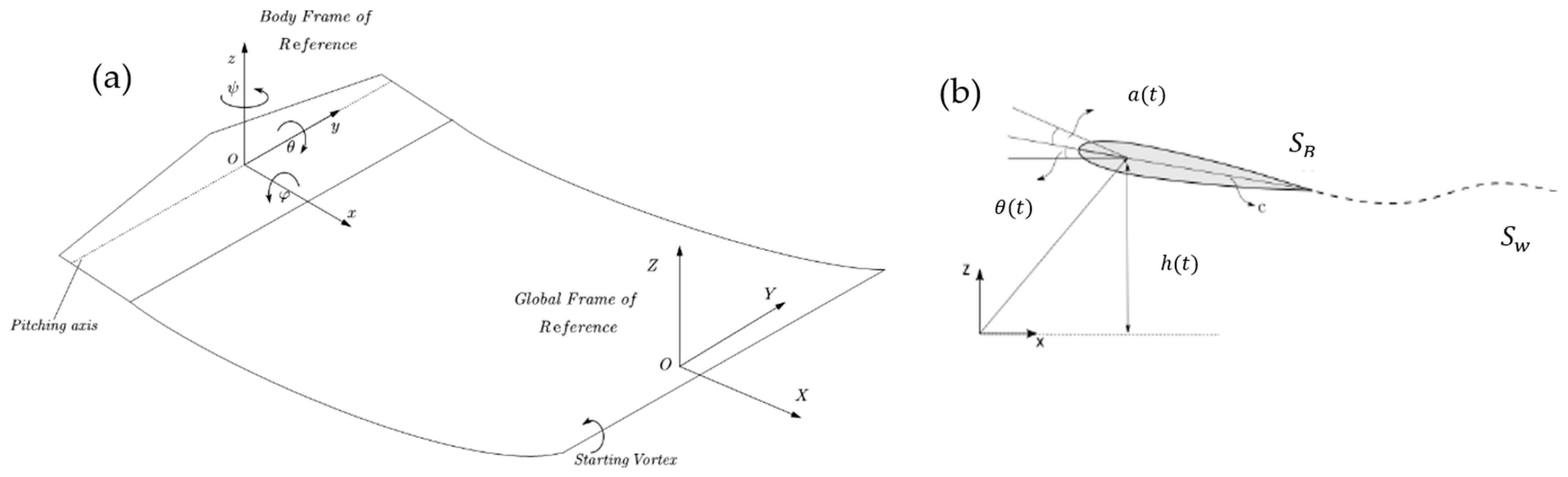
As a starting point, the flapping thruster is assumed to be submerged at increased depth within stationary liquid, travelling with constant speed U in the negative x-direction, as shown in Figure 2. In such a case, interactions between the wing and the vessel or the wavy free surface are considered to be negligible.

2.1. Flapping Wing Kinematics

The wing performs a combination of prescribed harmonic rigid-body motions (heaving and pitching at fixed phase difference). Specifically, for the description of the kinematical characteristics of the oscillating wing and of the induced flow dynamics, two reference systems are used. The inertial coordinate system is (X,Y,Z), and the body-fixed moving coordinate system is (x,y,z), which is translated with constant velocity U with respect to the former, simultaneously executing a combined heaving and angular oscillatory motion at the same frequency $\mathsf{\omega }=2\pi f$ (where f is the linear frequency), as depicted in Figure 2b.

In particular, the oscillatory motions are described by the following equations:

$$Z=h\left(t\right)=h_{0}sin\left(\mathsf{\omega }t\right),$$

(3)

$$\theta \left(t\right)={\theta }_0\sin \left(\omega t+\psi \right),$$

(4)

where $h_0$ and ${\theta }_0$ denote the amplitudes of heaving motion and pitching rotation, respectively. The angular motion lags the transverse one by a phase angle ψ = 90 deg.

In the present work, the most important non-dimensional parameters describing the kinematics due to their relevance to the dynamics of the wake are the Strouhal number $St=2f{h}_o/U$ and the maximum angle of attack

$${\mathsf{\alpha }}_0=max\left\{\left|\mathsf{\alpha }\left(t\right)\right|\right\},$$

(5)

where $\mathsf{\alpha }\left(t\right)$ denotes the instantaneous angle of attack

$$\mathsf{\alpha }\left(t\right)=ta{n}^{-1}\left({\displaystyle \frac{dh/dt}{U}}\right)-\theta \left(t\right).$$

(6)

2.2. Mathematical Modelling

By following the standard assumptions of the ideal model (see, e.g., [14,15]), the flow is considered attached, and the fluid around the oscillating wing is assumed to be inviscid and incompressible. The vorticity created in the boundary layers of the foil’s upper and lower surfaces is continuously shed into the wake modelled by trailing vortex sheets, and it is subsequently convected away from the wing with the local velocity. Specifically, the fluid velocity changes abruptly in magnitude and direction along the trailing vortex sheets, and the flow outside these surfaces is irrotational. Under the previous assumptions, the mathematical problem is formulated by the equations and boundary conditions as described below.

2.2.1. Governing Equation

The velocity field generated by the flapping wing and its wake is assumed to be irrotational and divergence-free; accordingly, it can be represented by a potential that exhibits a discontinuity on the lifting surface and the trailing vortex sheet. In addition, the disturbance velocity field, generated by the motion of the wing and the formation of its wake, must decay away from these boundaries, vanishing at infinity; see, e.g., Refs. [14,15]. The governing equation is the Laplace equation as derived from the continuity condition under the assumption of flow irrotationality

$${\nabla }^2\mathsf{\Phi }\left(X,Y,Z;t\right)=0,\left(X,Y,Z\right)\in D,$$

(7)

where D denotes the flow domain outside the foil and vortex wake.

2.2.2. Solid Boundary Condition

The solid boundary condition, which states that the velocity of the flow normal to the wing surface is zero, is applied by the following equation:

$$\left(\nabla \mathsf{\Phi }-{\mathit{U}}_{\mathit{B}}\right)\cdot \mathit{n}=0\mathrm{o}\mathrm{r}\nabla \mathsf{\Phi }\cdot \mathit{n}={\mathit{U}}_{\mathit{B}}\cdot \mathit{n},$$

(8)

where $\mathit{n}$ is the normal unit vector on the wing, and ${\mathit{U}}_{\mathit{B}}$ denotes the velocity due to the wing motion.

2.2.3. Kelvin Condition

Trailing vortex sheets must be force-free material surfaces, and the vorticity field (concentrated on these surfaces) must be divergence-free. Shed vorticity is convected with the local velocities as calculated at the nodal points of each free vortex ring. Also, by this technique, Kelvin’s theorem

$${\displaystyle \frac{D\mathsf{\Gamma }}{Dt}}=0$$

(9)

is automatically fulfilled, where Γ denotes the circulation around any closed material circuit, and D/Dt denotes the material derivative.

2.2.4. Kutta Condition

Among various alternative approximate forms of the Kutta condition in unsteady flow, in the present work, this condition is implemented by enforcing the vorticity generated at the trailing edge to shed with the local instantaneous flow velocity.

2.3. Numerical Scheme

By applying Green’s theorem, the general solution can be constructed by placing a sum of source $\sigma$ and doublet $\mu$ distributions placed on the wing boundary $S_B$,

$$\mathsf{\Phi }\left(X,Y,Z\right)=-{\displaystyle \frac{1}{4\pi }}{\int }_{S_B}\left[\sigma \left({\displaystyle \frac{1}{r}}\right)-\mu {\mathit{n}}_{{\mathit{x}}_0}\cdot {\nabla }_{{\mathit{x}}_0}\left({\displaystyle \frac{1}{r}}\right)\right]dS\left({\mathit{x}}_0\right)+{\displaystyle \frac{1}{4\pi }}{\int }_{S_w}\left[\mu {\mathit{n}}_{{\mathit{x}}_0}\cdot {\nabla }_{{\mathit{x}}_0}\left({\displaystyle \frac{1}{r}}\right)\right]dS\left({\mathit{x}}_0\right),$$

(10)

where $S_w$ denotes the trailing vortex wake.

The above equation does not use a specific combination of sources and doublets for a particular problem, which leads us to make a decision of high significance in this matter depending on the physics of the problem. It is clear that in order to model the effects of thickness, source elements are applied, whereas for lifting problems, antisymmetric terms such as the doublet (or vortex) can be used. However, the wake will be modelled by thin doublet or vortex sheets, and the thickness of the surface at the camber line is considered infinitesimal. Therefore no sources are used, and the potential equation can be rewritten as follows:

$$\mathsf{\Phi }\left(x,y,z\right)={\displaystyle \frac{1}{4\mathsf{\pi }}}{\int }_{S_{B}and{S}_W}\left[\mathsf{\mu }{\mathit{n}}_{{\mathit{x}}_0}\cdot {\nabla }_{x_0}\left({\displaystyle \frac{1}{r}}\right)\right]dS\left(x_0\right),$$

(11)

where ${\mathit{x}}_0$ denotes the position of the singularity elements. Substituting the new potential equation into the no-penetration condition (Equation (8)), the latter becomes the following:

$${\displaystyle \frac{1}{4\pi }}{\int }_{body+wake}\mu \mathsf{\nabla }\left[{\displaystyle \frac{\partial }{\partial n\left({\mathit{x}}_0\right)}}\cdot \left({\displaystyle \frac{1}{r}}\right)\right]\cdot \mathit{n}dS\left({\mathit{x}}_0\right)={\mathit{U}}_{\mathit{B}}\cdot \mathit{n}.$$

(12)

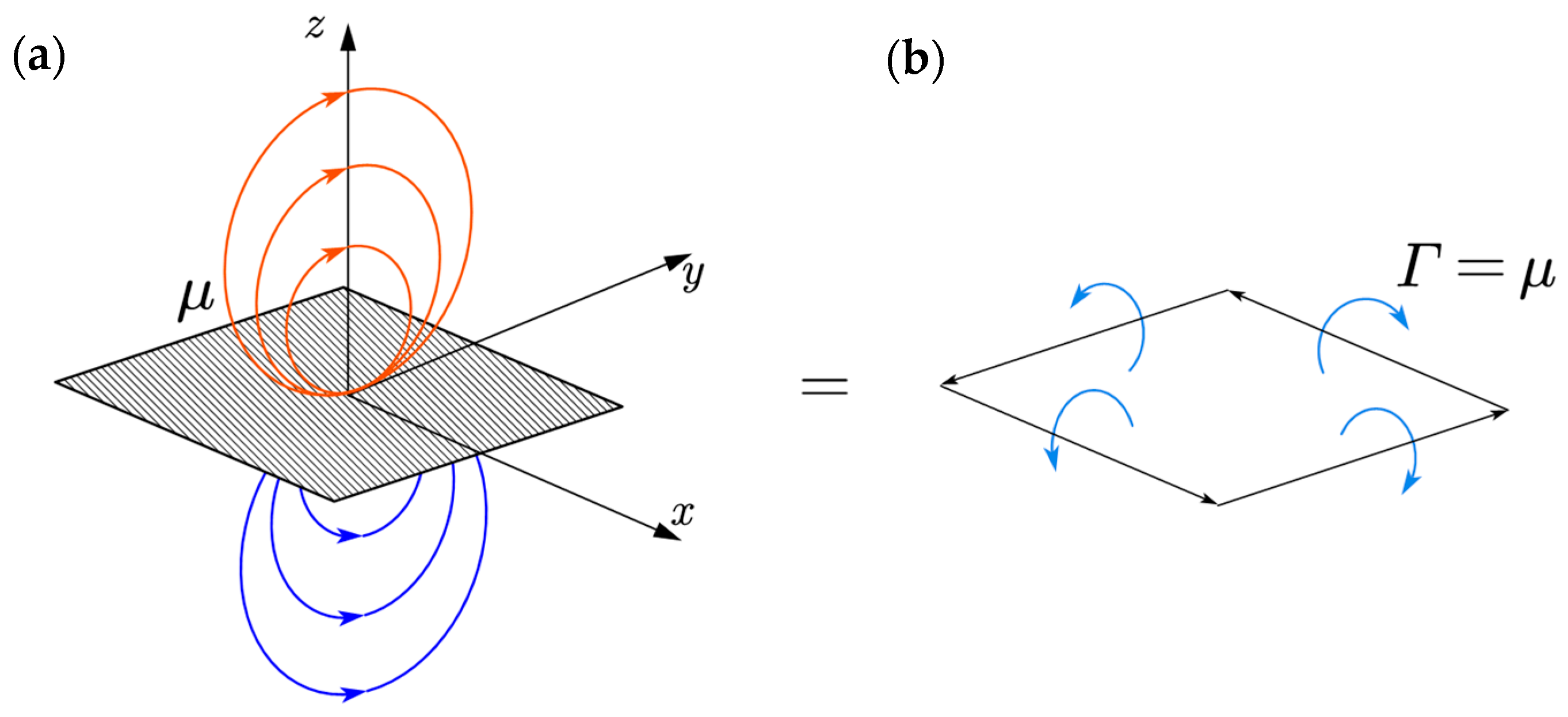
In the present work, the distributed singularity element that is chosen is only the vortex ring. Specifically, this choice is permitted due to the equivalence of the quadrilateral doublet element to the quadrilateral vortex ring element. In particular, the velocity induced at a point $P$ in the domain of interest by a quadrilateral doublet element of strength $\mathsf{\mu }$ is equivalent to the velocity induced by a vortex ring element of strength $\Gamma =\mu$; see Figure 3.

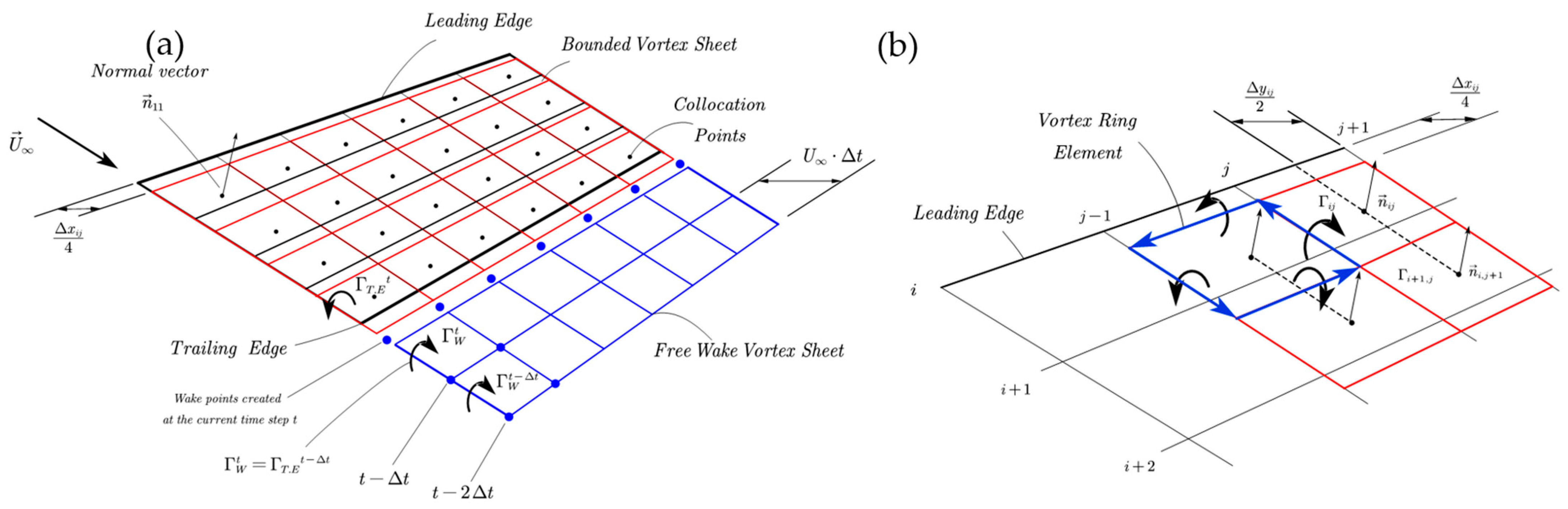
The numerical solution begins with dividing the lifting surface into N chordwise and M spanwise panels, as shown in Figure 4a. The normal vector on the wing $\mathit{n}$ is defined at the collocation points, which are denoted by the black dots located at the centres of the vortex ring elements, where the solid boundary condition is applied. A positive $\Gamma$ is defined here according to the right-hand rotation rule, as shown in Figure 4b. The front segment of the vortex ring is placed at the quarter of the chord of each panel so that the Kutta condition is satisfied.

Addressing the wake shedding procedure is crucial at this step. A vortex ring positioned on the last chordwise row of panels, as illustrated in Figure 4, is shed in the wake in the interval covered by the trailing edge during the latest time step with a length of $U\mathsf{\delta }t$. Based on the above and the discretization of the wing into vortex elements, the time step $\mathsf{\delta }t$ is selected so that the size of the wake elements are compatible with the corresponding elements near the trailing edge. The corner points of the wake vortex ring are generated at each time step. In the initial time step, only the two aft points of the vortex ring are created, meaning that there are no free wake elements at this stage. The trailing vortex segment of the trailing edge vortex ring serves as the starting vortex during the first time step.

In the subsequent time steps, as the wing’s trailing edge advances, a wake vortex ring is formed using the new points of the trailing edge vortex ring and the two points corresponding to the position at the previous time step; see Figure 4a. This shedding procedure repeats at each time step, resulting in a series of new trailing edge wake vortex rings being created (the wake shedding procedure).

The intensity of the wake vortex ring that is shed from the trailing edge of the flapping wing at each time step (as depicted in Figure 4a) is equal to the strength of the vortex being shed ${\mathsf{\Gamma }}_{T.E}^{t-\mathsf{\Delta }t}$ at the preceding time step. This process, in conjunction with the discrete representation of the wing and wake by vortex elements, as shown in Figure 4a, guarantees the satisfaction of the Kutta condition in discrete form, modelling the shedding of vorticity from the wing to the trailing vortex wake and its subsequent transport with the local velocity; see also Katz & Plotkin (Ref. [14], Section 13.12).

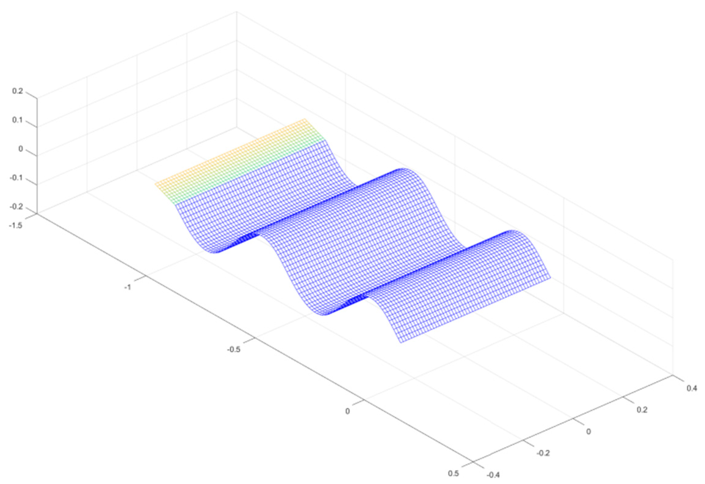
Upon shedding the wake vortex ring elements, their strength remains constant, and the vortex wake surface is modelled as a free vortex sheet moving in accordance with the local velocity, also satisfying Kelvin’s law, Equation (9), in discrete form, as illustrated in Figure 5. In general, the free trailing vortex sheet is also subject to deformation due to the effects of self-induced velocity. However, considering that the deformation becomes more significant in larger distances from the wing, the trailing vortex sheet geometry is well approximated in the first part near the trailing edge, and its effects on the wing are well represented by the above process. The effects of trailing deformation are left to be included in future extensions of the present model, in cases of applications of multiple flapping wings arranged in a row, where the interaction is expected to be important.

2.4. Calculation of Vortex Element Strength on Wing

The calculation of vortex strengths, for all elements on the wing ${\Gamma }_{i_{el}},i_{el}=\mathrm{1,2},\dots ,M\times N,$ requires the solution of a system of equations materializing the no-entrance boundary condition, Equation (8). First, we recall the boundary condition (Equation (8)), which, after discretization and the implementation of the previously presented numerical scheme, takes the following form:

$${\sum }_{i_{el}=1}{A}_{i_{cp},i_{el}}{\Gamma }_{i_{el}}+{\sum }_{i_{el}=1}{A^W}_{i_{cp},i_{el}}{{\Gamma }^w}_{i_{el}}={\mathit{U}}_{\mathit{B},i_{cp}}\cdot {\mathit{n}}_{i_{cp}},i_{cp}=\mathrm{1,2},\dots ,M\times N,$$

(13)

where $A_{i_{cp},i_{el}}{{\mathrm{a}\mathrm{n}\mathrm{d}A}^W}_{i_{cp},i_{el}}$ denote the influence matrices of the vortex ring element with unit strength to the normal velocity at the centroids of the wing panels, where the index $i_{cp}$ corresponds to the collocation point, and $i_{el}$ represents the vortex ring element inducing velocity at that location. The second term on the left-hand side of the equation represents the contribution of wake elements to the total induced velocity. Since their strengths were determined in the previous time step, this term is transferred to the right-hand side of the equation. Applying this relation at each time step $t_n,n=\mathrm{1,2},\dots ,$ and all collocation points $i_{cp}=\mathrm{1,2},\dots ,MxN,$ forms the following system of equations:

$${\sum }_{i_{el}=1}{A}_{i_{cp},i_{el}}{\Gamma }_{i_{el}}\left(t_n\right)=B_{i_{cp}}\left(t_n\right),i_{cp}=\mathrm{1,2},\dots ,MxN,n=\mathrm{1,2},\dots .$$

(14)

where $B_{i_{cp}}\left(t_n\right)={\mathit{U}}_{\mathit{B},i_{cp}}\left(t_n\right)\cdot {\mathit{n}}_{i_{cp}}-{\sum }_{i_{el}=1}{A^W}_{i_{cp},i_{el}}{{\Gamma }^w}_{i_{el}}$. The above system is then solved at each time step $t_n$ to determine the unknown strengths ${\Gamma }_{i_{el}}\left(t_n\right),i_{el}=\mathrm{1,2},\dots ,M\times N$.

2.5. Calculation of Wing Pressure and Loads

Using Bernoulli’s equation in discrete form, the pressure difference (pressure jump) on the wing is calculated at each vortex ring element $i_{el}=(i,j)$,

$$\Delta p_{i,j}=\rho \left({[U_{rel}+u_w,V_{rel}+v_w,W_{rel}+w_w]}_{i_{el}}\cdot \left[\begin{array}{c}cos\left(\theta \left(t\right)\right)\\ 0\\ -sin\left(\theta \left(t\right)\right)\end{array}\right]\cdot {\displaystyle \frac{{\Gamma }_{i,j}-{\Gamma }_{i-1,j}}{\Delta c_{i,j}}}+{\displaystyle \frac{\partial }{\partial t}}{\Gamma }_{i,j}\right),$$

(15)

where $\mathsf{\rho }$ is the water density ${\left[U_{rel},V_{rel},W_{rel}\right]}_{i_{el}}=-{\mathit{U}}_{\mathit{B}{i}_{el}}$, and ${\left[u_w,v_w,w_w\right]}_{i_{el}}$ denotes the induced velocities from the trailing vortex wake at the centroid of each wing element. Subsequently, the panel forces acting on the foil are calculated as follows:

$$\Delta L_{i,j}=-\Delta p_{i,j}\cdot \Delta S_{i,j}\cdot cos\left(\theta \right),$$

(16)

$$\Delta D_{i,j}=\Delta p_{i,j}\cdot \Delta S_{i,j}\cdot sin\left(\theta \right),$$

(17)

where $\Delta S_{i,j}$ denotes the element surface, and the hydrodynamic forces $F_x$ $\mathrm{a}\mathrm{n}\mathrm{d}{F}_z\mathrm{a}\mathrm{r}\mathrm{e}\mathrm{o}\mathrm{b}\mathrm{t}\mathrm{a}\mathrm{i}\mathrm{n}\mathrm{e}\mathrm{d}$ by integration on the wing surface $S_B$. In particular, the total instantaneous forces and moments for each time step are computed by adding the contribution of each individual vortex ring element. The time-averaged mechanical power $\overline{P}$ required to generate the foil’s combined oscillatory motion, or input power, is obtained as the mean value over a period of oscillation (at the end of simulation):

$$\overline{P}={\displaystyle \frac{1}{nT}}{\int }_0^T\left(F_z\left(t\right)\dot{h}\left(t\right)+M\left(t\right)\dot{\theta }\left(t\right)\right)dt.$$

(18)

and similarly, the time-averaged values of the wing forces ${\overline{F}}_x\mathrm{a}\mathrm{n}\mathrm{d}$ ${\overline{F}}_z\mathrm{a}\mathrm{r}\mathrm{e}\mathrm{c}\mathrm{a}\mathrm{l}\mathrm{c}\mathrm{u}\mathrm{l}\mathrm{a}\mathrm{t}\mathrm{e}\mathrm{d}$

$${\overline{F}}_z={\displaystyle \frac{1}{nT}}{\int }_0^T{F}_z\left(t\right)dt,{\overline{F}}_x={\displaystyle \frac{1}{nT}}{\int }_0^T{(F}_x\left(t\right){-F}_d\left(t\right))dt,$$

(19)

$\mathrm{w}\mathrm{h}\mathrm{e}\mathrm{r}\mathrm{e}{F}_d\left(t\right)=0.5\rho U^{2}S{C}_d$ is used for viscous corrections using the empirical drag coefficient $C_d$ based on the Reynolds number and the instantaneous angle of attack a(t) given by Equation (6). The above approximation is used for viscous correction in ideal flow models; see, for example, Ref. [9]. The time integrals in Equation (19) are calculated numerically, and time averaging is performed after 4–5 cycles of oscillation, which is found to be enough for numerical convergence. By this point, the wake shedding process is fully developed, and the foil’s operation has reached steady conditions, ensuring that the estimation of the mean input power is accurate.

Finally, the $\mathrm{t}\mathrm{h}\mathrm{r}\mathrm{u}\mathrm{s}\mathrm{t},\mathrm{l}\mathrm{i}\mathrm{f}\mathrm{t}$, and power coefficients a $C_x$,$C_L$, and $C_P$ are obtained, respectively,

$$C_x={\displaystyle \frac{{\overline{F}}_x}{\frac{1}{2}\rho U^2\cdot S}},$$

(20)

$$C_L={\displaystyle \frac{{\overline{F}}_z}{\frac{1}{2}\rho U^2\cdot S}},$$

(21)

$$C_P={\displaystyle \frac{\overline{P}}{\frac{1}{2}\rho U^3\cdot S}},$$

(22)

where S is the wing’s planform area. Consequently, the hydrodynamic propulsive efficiency $\eta$ is calculated by the following:

$$\eta ={\displaystyle \frac{{\overline{F}}_x\cdot U}{\overline{P}}}={\displaystyle \frac{C_x}{C_P}}.$$

(23)

2.6. Leading Edge Suction Correction

Since the model used in the present analysis corresponds to thin lifting surface, a considerable percentage of the thrust force is contributed by the leading edge suction force. The latter force results from the low-pressure region created by the high-speed flow at the leading edge. Consequently, it is important to supplement the present numerical model with corrections concerning the leading edge suction force. It is known that the velocity at the leading edge contains an inverse square root singularity. Therefore, it is difficult to estimate the force correctly by applying numerical pressure integration. In this work, the methodology in [16] is implemented, based on the calculation of the mean sectional leading edge thrust coefficient $c_t$ of each chordwise strip as follows:

$$c_t={\displaystyle \frac{t_l}{\frac{1}{2}\mathsf{\rho }{s}_l{U}^2}}={\displaystyle \frac{1}{2}}\mathsf{\pi }{\displaystyle \frac{{C_S}^2}{2cos\mathsf{\Lambda }}},$$

(24)

where $t_l$ is the sectional leading edge suction force, $\mathsf{\Lambda }$ is the leading edge sweep angle, and s stands for the area of the longitudinal strip. In Equation (24), $C_S$ is a parameter that represents the leading edge singularity, defined as follows:

$$C_s=\underset{x\to x_{\mathit{LE}}}{\lim }2u\left(x\right)\cdot {\left({\displaystyle \frac{x-x_{LE}}{c}}\right)}^{{\displaystyle \frac{1}{2}}},$$

(25)

where $u$ is the horizontal non-dimensional flow velocity at the leading edge, and x is the distance from the leading edge position $x_{LE}$. According to [16], the parameter $C_s$ can be calculated numerically in the vortex element approach using the following:

$${\displaystyle \frac{1}{2}}{N}_C{C}_S{D}_S=\sum \left(\mathrm{upwash}\mathrm{at}\mathrm{leading}\mathrm{edge}\right)-w\left(x_{LE},y_{LE}\right),$$

(26)

with

$$D_S=2{\left(\mathrm{t}\mathrm{a}{\mathrm{n}}^2\mathsf{\Lambda }+1\right)}^{1/2},$$

(27)

where Nc is the number of panels on the strip of the wing, and $w\left(x_{LE},y_{LE}\right)$ stands for the lateral velocity at the corresponding point of the leading edge. According to the above model, upwash is defined as the total vertical velocity at the leading edge, induced by the wing’s vortex ring elements; see also [17]. The total leading edge suction force $T_S$ is estimated by integrating the sectional leading edge suction force $t_l$ over the span of the flapping wing. Consequently, the total thrust force is corrected by including the leading edge suction force $T_S$ in the horizontal force $F_x\left(t\right)$ computed from the numerical integration of pressure difference across the wing.

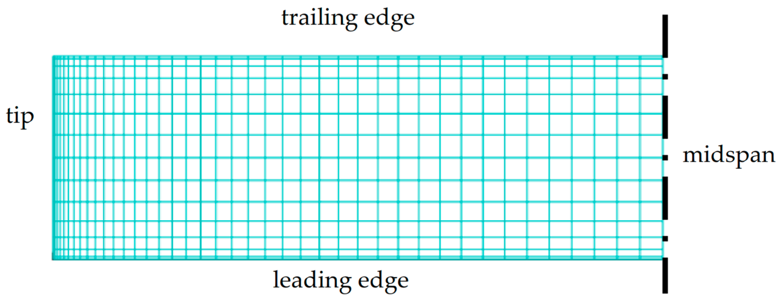
To correctly estimate the asymptotic behaviour of the flow near the leading edge, an iso-cosine mesh is employed. More specifically, the mesh has higher density near the leading edge, the trailing edge, and the tip of the flapping wing; see Figure 6 in the case of a wing with an orthogonal planform. The increased mesh density helps to accurately capture the leading suction force. Additionally, it is important to select the time step such that the vortex rings in the vicinity of the trailing edge of the wing have comparable lengths with the panels in the wake in order to ensure that the wake shedding from the trailing edge is accurately modelled.

2.7. Numerical Results and Verification

In this section, the validity of the present method is demonstrated by comparing the numerical results with the experimental data from [2]. The comparison concerns a flapping foil thruster with the following characteristics:

• $c=0.1\mathrm{m}$ mid-chord length.
• $s=0.6\mathrm{m}$ wingspan length.
• $U=0.4\mathrm{m}/\mathrm{s}$.
• ${\displaystyle \frac{X_P}{c}}=0.33$, where $X_P$ is the position of the pivot axis measured from the leading edge.
• $St=0.3$ Strouhal number.
• ${\mathsf{\theta }}_0=2.23°$.
• $\mathsf{\psi }=90°$ phase lag of pitching oscillation.
• ${\displaystyle \frac{h_0}{c}}=0.75$.

The experiments were conducted using a symmetric rectangular foil of a constant NACA 0012 section; see [18]. It is essential to state that the three-dimensional effects were limited by placing two circular endplates of 0.35 m diameter at each end of the foil.

The present method is found to be very rapidly convergent. A comparison of the calculated results regarding the time history of the thrust and lift coefficients against experimental data from [2] is presented in Figure 7. It is noted that the numerical results are obtained using a mesh of 42 spanwise elements (along the wing semispan) by 14 chordwise elements, which is shown to be enough for numerical convergence. More specifically, lines are used to indicate the present model’s predictions, while experimental measurements are shown by using dashed lines and open circles.

The results presented were generated during the last two periods of the oscillatory motion of the flapping foil, and in general, good agreement is observed. Small differences are observed near the peaks of the thrust coefficient, which are due to the approximation introduced by the above suction force model used to describe the leading edge flow behaviour. It is also noted that these results were obtained using a 3D wing with a large aspect ratio in order to better simulate the experimental measurements.

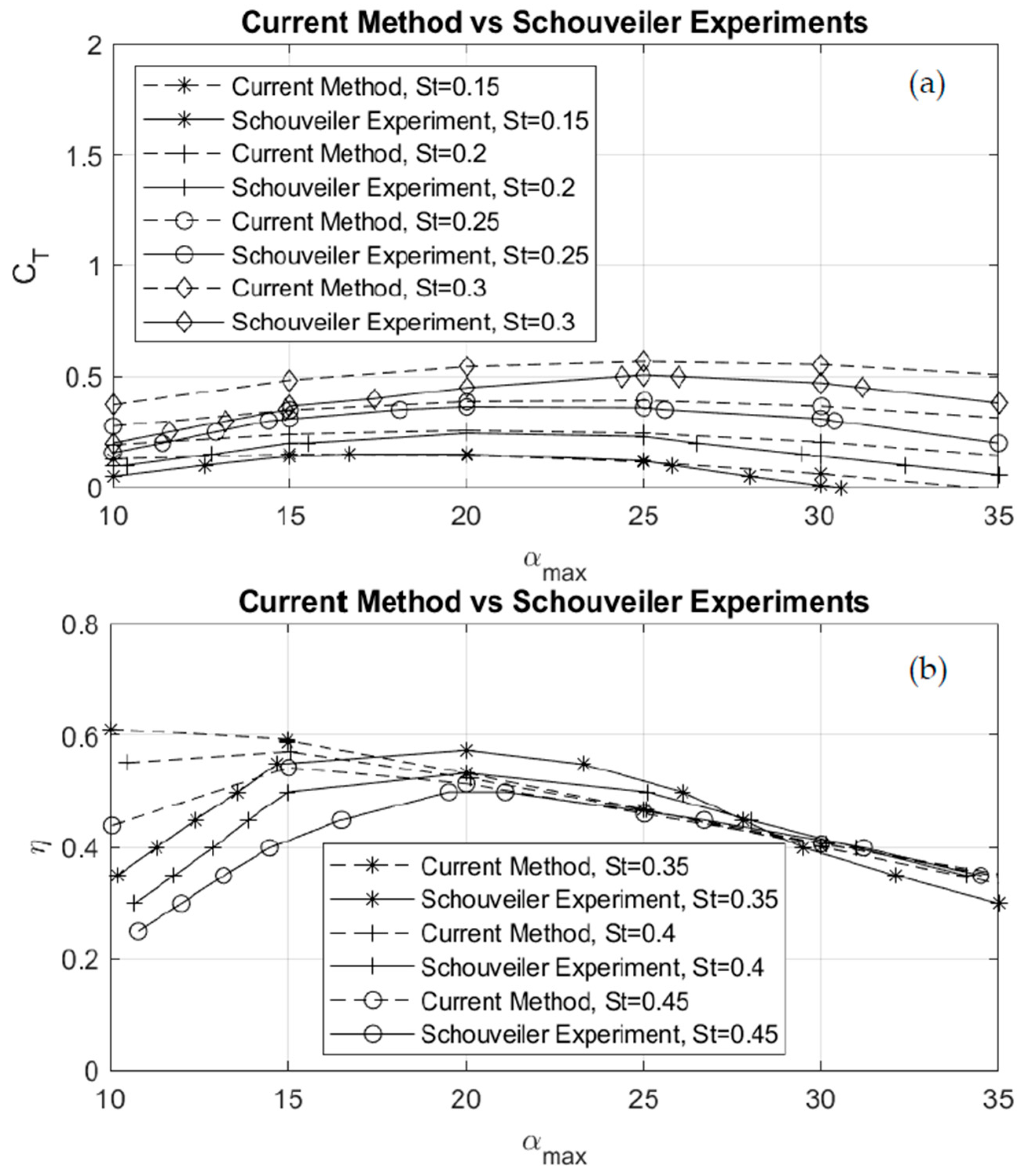
Further comparisons with the experimental data from [2] are presented in Figure 8 for other operational conditions of the flapping foil. In this figure the mean thrust coefficient and efficiency of the flapping foil are shown as a function of the maximum angle of attack for various Strouhal numbers ranging from 0.15 to 0.45.

Regarding the mean thrust coefficient, the numerical results obtained by the present method are found to be in good agreement with experimental measurements for the maximum angles of attack below 25 deg and Strouhal numbers between 0.15 and 0.25. However, deviations occur in cases of higher unsteadiness and large angles of attack, since nonlinear effects and more pronounced viscous flow effects associated with flow separation are neglected by the present model.

Regarding efficiency estimation, it is evident that in the range of the maximum angles of attack α_max = 10°–15°, the current method presents a trend of overestimating efficiency due to the increased estimation of the mean thrust coefficient in this range of operation parameters.

On the other hand, in the range of α_max = 15°–25°, the present method tends to slightly underestimate efficiency. In general, we observe that although the present simplified model does not precisely predict efficiency, the calculation curves exhibit similar trends and effectively capture the influence of the Strouhal number and angle of attack on both the thrust and efficiency of the flapping wing. Therefore, the present method, characterized by simplicity in modelling and low computational cost, is considered to be suitable for the preliminary design of the considered flapping foil propulsion system, especially in more complicated operating conditions, as will be discussed in Section 3.

2.8. Verification by Comparison with 2D Linear Theory for Thin Foils

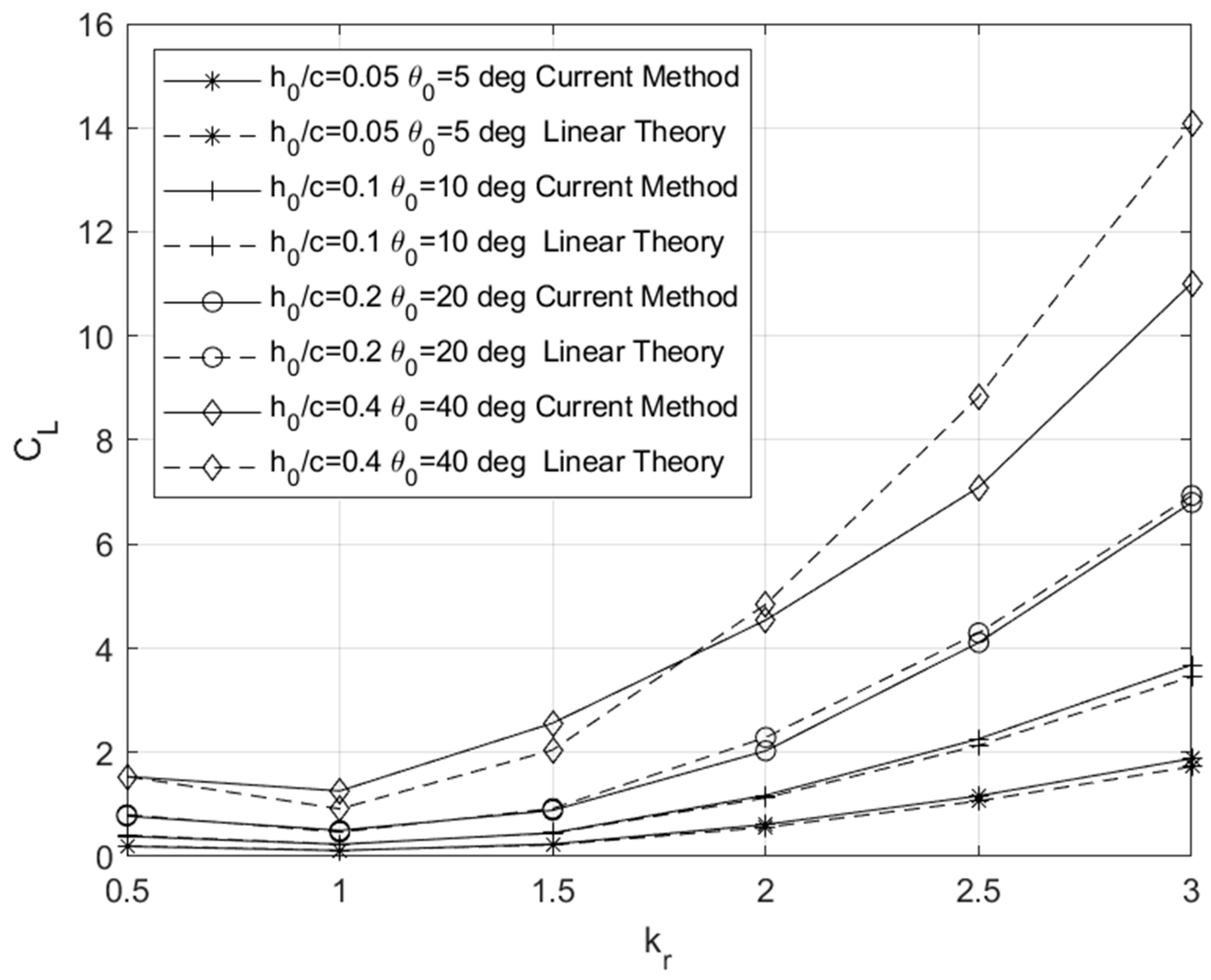
In order to verify the present method, additional comparisons will be presented with results from unsteady thin airfoil theory. This will further confirm the present model’s reliability across a wide range of frequencies and amplitudes. As an example, the results are presented in Figure 9 using a wing of an orthogonal planform with a very large aspect ratio. In particular, the results concern the amplitude of the lift coefficient in flapping motion estimated by the present method and the linear theory for the following parameters: $h_0/c=0.05÷0.4$, ${\theta }_0=5°÷40°$, $\psi =90°$, and the position of the pivot axis in the middle of the chord, pic = 0.5. The observed agreement of the present model with theoretical predictions is very good, and deviations occur only at large oscillation amplitudes, as expected, since linear theory is valid only for small oscillation amplitudes.

In Figure 9 the lift coefficient is presented as a function of the reduced frequency

$$k_r={\displaystyle \frac{\mathsf{\omega }\cdot c}{2\cdot U}}.$$

(28)

Specifically, the integrated results concerning the amplitude of the lift coefficient obtained using the present method are compared with predictions from the linearized theory for thin uncambered hydrofoils. In these comparisons, the hydrofoil, represented by a flat plate, is performing small and moderate oscillations. The lift coefficient according to linear theory is calculated through

$$L=\mathsf{\pi }\mathsf{\rho }UcC\left(k_r\right)\left[U\cdot \mathsf{\theta }-\dot{h}+\left({\displaystyle \frac{3}{4}}-pic\right)c\cdot \dot{\mathsf{\theta }}\right]+\mathsf{\pi }\mathsf{\rho }{\displaystyle \frac{c^2}{4}}\left[\left(U\dot{\mathsf{\theta }}-\ddot{h}\right)+c\left({\displaystyle \frac{1}{2}}-pic\right)\ddot{\mathsf{\theta }}\right],$$

(29)

where pic denotes the location of the pivot axis along the chord of the foil; see also [14]. This formula easily accounts for the effects of the pitching axis pivot position relative to the chord, and C(k_r) denotes the Theodorsen function:

$$C\left(k_r\right)={\displaystyle \frac{H_1^{\left(2\right)}\left(k_r\right)}{H_1^{\left(2\right)}\left(k_r\right)+i\cdot H_0^{\left(2\right)}\left(k_r\right)}}.$$

(30)

where $H_{\mathrm{0,1}}^{\left(2\right)}\mathrm{d}\mathrm{e}\mathrm{n}\mathrm{o}\mathrm{t}\mathrm{e}\mathrm{s}\mathrm{t}\mathrm{h}\mathrm{e}\mathrm{H}\mathrm{a}\mathrm{n}\mathrm{k}\mathrm{e}\mathrm{l}\mathrm{f}\mathrm{u}\mathrm{n}\mathrm{c}\mathrm{t}\mathrm{i}\mathrm{o}\mathrm{n}\mathrm{o}\mathrm{f}\mathrm{s}\mathrm{e}\mathrm{c}\mathrm{o}\mathrm{n}\mathrm{d}\mathrm{k}\mathrm{i}\mathrm{n}\mathrm{d}\mathrm{a}\mathrm{n}\mathrm{d}\mathrm{o}\mathrm{r}\mathrm{d}\mathrm{e}\mathrm{r}\mathrm{s}\mathrm{0,1},\mathrm{r}\mathrm{e}\mathrm{s}\mathrm{p}\mathrm{e}\mathrm{c}\mathrm{t}\mathrm{i}\mathrm{v}\mathrm{e}\mathrm{l}\mathrm{y}.$ The ratio $C$(k_r) accounts for the memory effect of the unsteady wake. Since the above theoretical results refer to a 2D foil, in order to limit the three-dimensional effects in the present model, an aspect ratio of AR = 20 is used to obtain the approximation of the results presented in Figure 9.

3. Performance of Bow T-Foil Thruster in Irregular Waves

The theory of fish propulsion has proven to have significant practical applications. Except for when operating as a self-propulsion system of a ship or AUV, the dynamic wing has shown significant advantages for augmenting ship propulsion in waves; see [19,20]. In particular, tank experiments conducted at the towing tank of NTUA have demonstrated an average pitch and heave reduction of 30% and 15%, respectively, and a reduction in delivered power of up to 30% for regular head waves near the resonance. This was reported in the case of a ferry ship model with an actively controlled flapping thruster; see [21,22]. In addition, similar experimental results were provided by [23] where a free-running model with a spring-loaded foil system demonstrated a reduction in delivered power of up to 50% in regular head waves and an estimated reduction of 12% in irregular head waves with directional spreading.

Based on the previous findings, a promising approach to reducing resistance in waves and carbon emissions is the installation of foil thrusters below the bow of the ship. These thrusters extract wave energy and convert it directly into thrust, also providing dynamic stability and reducing added wave resistance. The extracted energy is effectively transformed into forward propulsion, demonstrating a novel method of improving the fuel efficiency of maritime vessels. However, constructing such a mechanism on the large scale required by the shipping industry is undoubtedly challenging. As a result, an alternative design based on a T-foil at the bow of the ship, as shown in Figure 10, could offer a more feasible alternative.

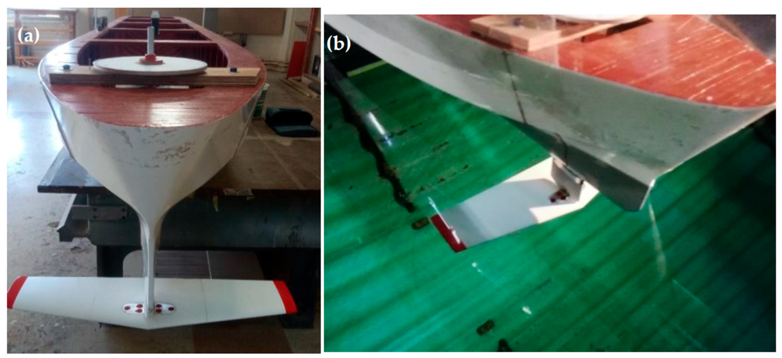
The numerical method analyzed in the previous sections was further extended for foils undergoing a more general heaving and pitching oscillatory motion. However, with some modifications, it can be adjusted to predict the hydrodynamic performance of a T-foil under real sea state conditions. As mentioned before, the T-foil is fixed to the ship, and thus it follows the exact motions of the ship in each sea state. In order to investigate the behaviour of the T-foil at the bow of the ship, as concerns thrust augmentation in waves, the wing shown in Figure 11 was used in a 3.3 m long model of a ferry ship and tested in the towing tank of NTUA, with dimensions of 100 m length, 4.6 m breadth, and depth 3 m, and the present method was used to obtain and compare the results in irregular head waves with experimental measurements, as described below. The towing tank was equipped with a running carriage that can achieve a maximum speed of 5.5 m/s. In addition, a single direction wave maker was used, capable of producing head waves with a frequency between 0.3 and 1.2 Hz and a maximum amplitude of 35 cm.

The model was attached to the dynamometer through a trim pivot, located longitudinally at the centre of gravity and transversely at the centre line. At the axle of the pivot, sensors were installed for the measurement of the dynamic responses.

3.1. Numerical Simplified Method Under Irregular Wave Conditions

In the present work, linear wave theory is applied, assuming fully developed sea conditions with wave amplitudes that are small compared to the wavelength. The irregular wave conditions are modelled by using the Bretschneider frequency spectrum providing the distribution of wave energy in the frequency domain.

In particular, the wave spectrum in the earth-fixed reference system is denoted as $S\left(\omega \right)$ and is given by

$$S\left(\omega \right)={\displaystyle \frac{1.25}{4}}{\displaystyle \frac{{\omega }_P^4}{{\omega }^5}}{H}_s^{2}exp\left(-1.25{\left({\displaystyle \frac{{\omega }_P}{\omega }}\right)}^4\right),$$

(31)

where the modal (peak) period $T_p=2\pi /{\omega }_p$ for various sea states with the severity characterized by the significant wave height $H_s$. Moreover, in the present work, the encounter frequency is considered to estimate the foil’s hydrodynamic performance. This is because the foil responds to incident bow waves at the encounter frequency ${\omega }_e$. Thus, it is necessary to calculate the wave spectrum from the perspective of a moving observer with the foil’s mean velocity U. This is obtained using the following relation:

$$S^U\left({\omega }_e\right)=S\left(\omega \right){\displaystyle \frac{d\omega }{d{\omega }_e}},\mathrm{w}\mathrm{h}\mathrm{e}\mathrm{r}\mathrm{e}{\omega }_e=\omega +kU\mathrm{and}k={\displaystyle \frac{{\omega }^2}{g}},$$

(32)

obtaining the following relation:

$$S^U\left({\omega }_e\right)=S\left(\omega \right)\cdot {\left(1+{\displaystyle \frac{2\omega U}{g}}\right)}^{-1}.$$

(33)

In order to acquire the spectrum of the wing’s vertical motion, the Response Amplitude Operator (RAO) of ship bow motion is used. Specifically, this is equal to the following:

$$S_{foil}^U\left({\omega }_e\right)=S^U\left({\omega }_e\right)\cdot {\left|RA{O}_{foil}\left({\omega }_e\right)\right|}^2,$$

(34)

where the RAO is defined as follows:

$$RAO={\displaystyle \frac{{\xi }_3-x_{wing}{\xi }_5}{A}}.$$

(35)

In Equation (35),

• ${\xi }_3$ is the ship’s heaving (vertical displacement) response to incident waves.
• $x_{wing}$ is the wing’s longitudinal distance from the pitching axis.
• ${\xi }_5$ is the ship’s pitching response to incident waves.
• $A$ is the wave amplitude.

The vertical motion of the T-foil is described by the random phase model. The band of encounter frequencies is discretized into a large number of consecutive bins of width $\delta \omega$ centred at the discrete values ${\omega }_{e,n}$.

$$h\left(t\right)=\sum _n{h}_{n}cos\left({\omega }_n+{ϵ}_n\right){,h}_n=\sqrt{2S_{foil}^U\left({\omega }_{e,n}\right)\delta {\omega }_e},$$

(36)

where ${ϵ}_n$ represents random phases that are uniformly distributed in $\left[\mathrm{0,2}\pi \right).$

3.2. Experimental Set Up

To assess the reliability of this simplified numerical model, experimental data from [20] are used. All tests were conducted in the towing tank of the Laboratory for Ship and Marine Hydrodynamics (LSMH) of the National Technical University of Athens (NTUA), which has a length of 91 m, width of 4.55 m, and max water depth 3 m; see Figure 12. Two irregular wave tests were conducted for one loading condition, at two speeds (1.20 m/s and 1.42 m/s), with Hs = 6 cm and 7 cm with a peak period of Tp = 1.35 s and 1.5 s, respectively, covering realistic moderate sea state conditions.

Our numerical model was tested for a ship model encountering random head waves, at a speed of U = 1.20 m/s (corresponding to Froude number Fr = 0.25) with a significant wave height Hs = 7 cm and peak period T_p = 1.5 s (0.67 Hz). The length of the model is 3 m, and a T-foil with geometry as depicted in Figure 10 and dimensions and data as given in Figure 11 is arranged at the bow. It is first observed in Figure 13 that the presence of the T-foil remarkably reduces the vertical (heaving) oscillation of the ship model, which is expected to cause a reduction in the mean added wave resistance and stabilization of the ship in waves.

The experimental results showed that the total mean resistance of the ship model in the above condition decreased from $R=0.620kp$ to $R_f=0.594kp$ when using a T-foil. Consequently, the contribution of the T-foil to the ship resistance reduction is estimated as follows:

$$C_{T-foil}={\displaystyle \frac{0.620kp-0.594kp}{\frac{1}{2}\rho U^{2}S}}=0.0057$$

(37)

3.3. Verification of Present Vortex Element Model

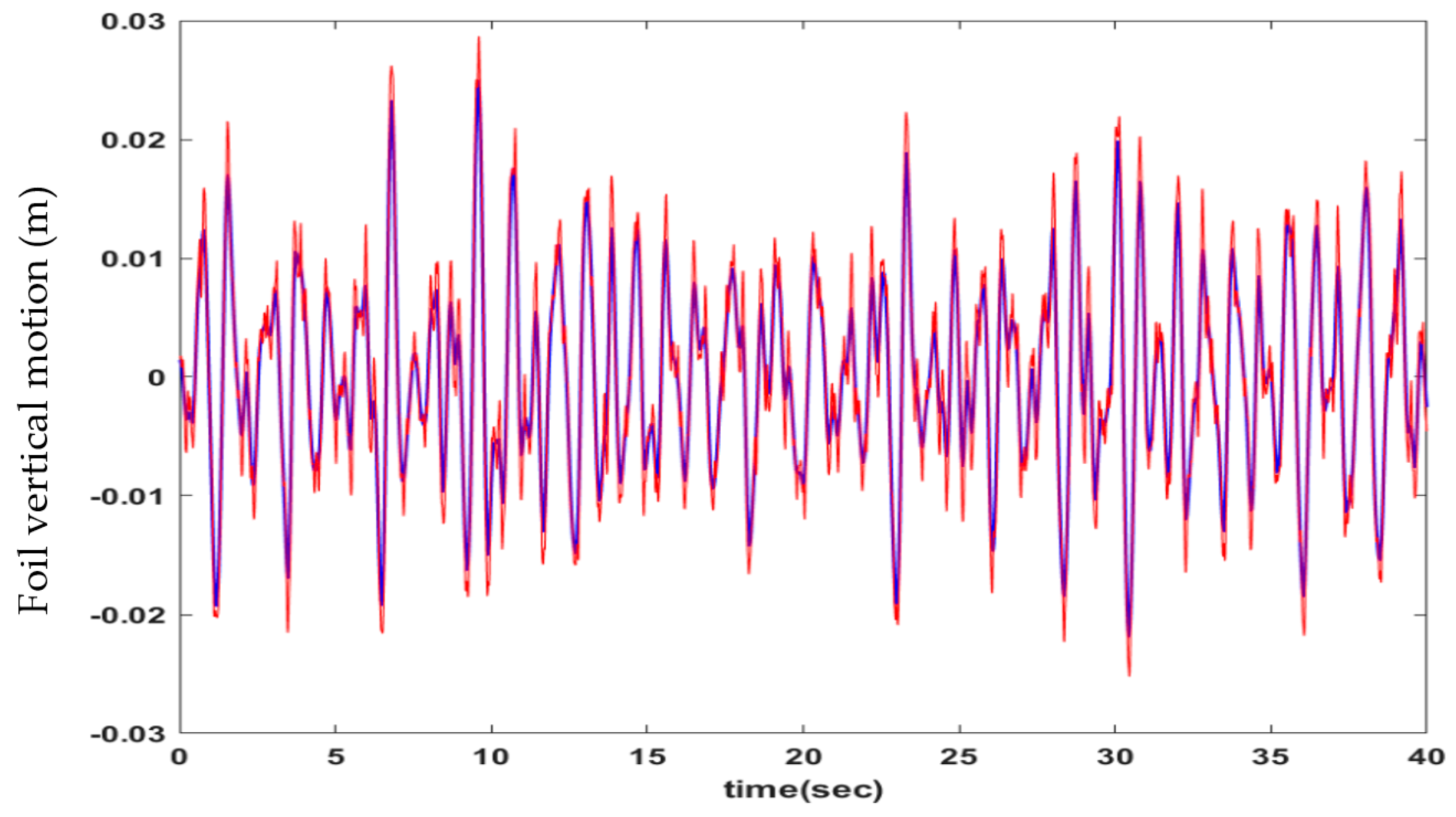
The heaving vertical motion of the bow T-foil is generated using the Bretschneider spectral model, Equation (31), with H_s = 3.5 cm and T_p = 1.5 s, which matches the profile of the heave oscillations shown in Figure 14, for a time interval of many characteristic peak periods. The simulated data are used to estimate the thrust coefficient $C_x$ of the foil undergoing the above vertical oscillations. A filtering scheme is employed to remove high-frequency noise in the simulated time series, thus avoiding the instabilities and excessive computational cost associated with the time step required for the numerical convergence of the present model.

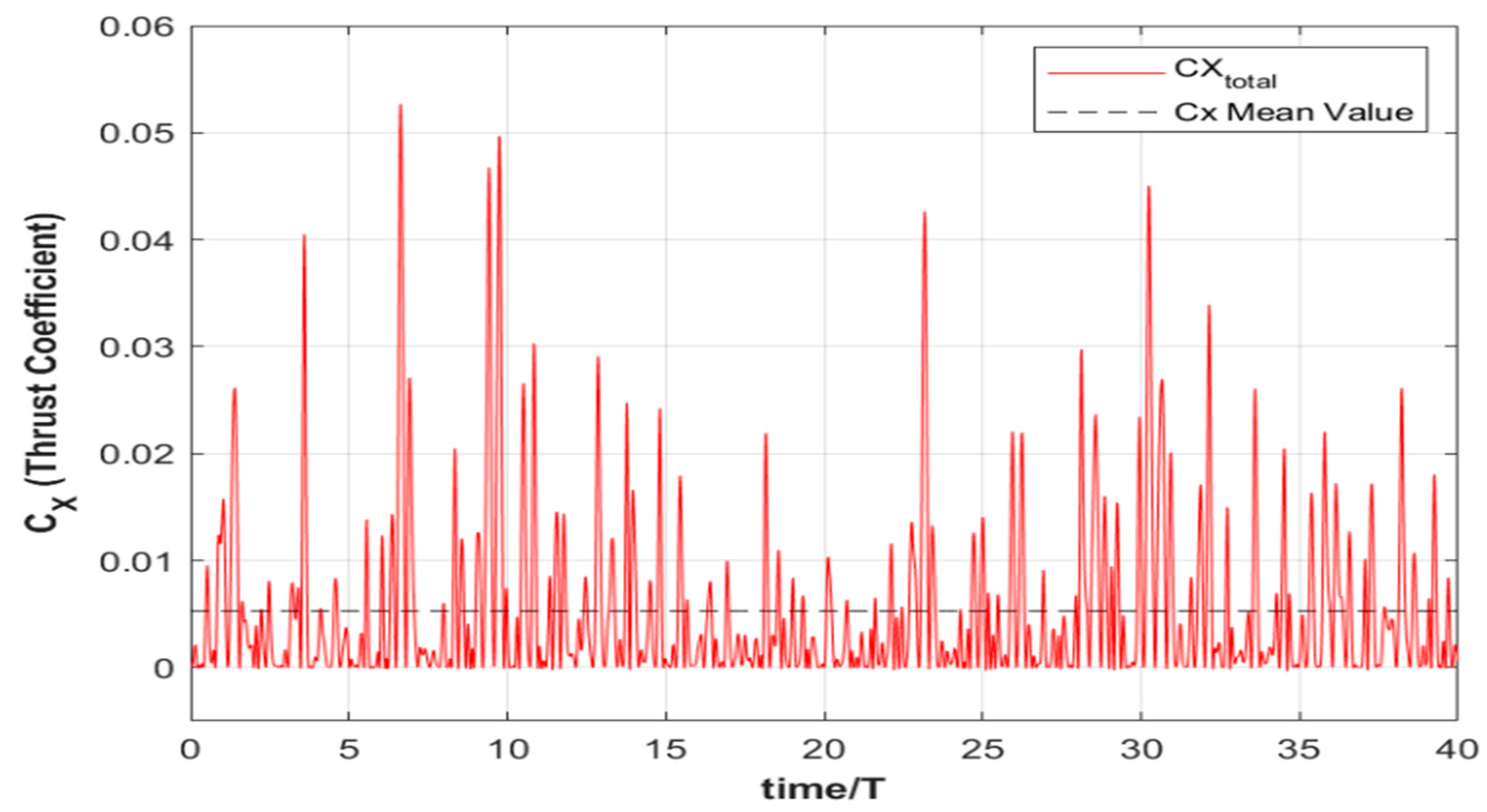
The present model is used in conjunction with the simulated vertical motion of the T-foil, and the results concerning the calculated time series of the thrust coefficient during the 40 peak periods are plotted in Figure 15, from which the following mean value is obtained

$$\overline{C_x}=0.0053$$

(38)

as also indicated in Figure 15 by using a dashed line. This predicted value matches the experimental measurement, confirming the validity of the numerical method. The above numerical experiment was performed multiple times to check its repeatability. The mean thrust values are $C_X^1=0.0055,C_X^2=0.0050,C_X^3=0.0054,C_X^4=0.0051,C_X^5=0.0052,C_X^6=0.0053$, verifying the above prediction of the thrust generated by the bow T-foil operating in flapping mode, as induced by the ship’s responses to waves.

The experimental study of the examined system in irregular head waves conducted in a towing tank is subject to limitations when compared to real sea conditions. To extend the experimental analysis, the development of large-scale models and testing in open-sea conditions, as described by Belibassakis in Ref. [24], could provide useful data for evaluating the combined performance of the foil thruster with the propulsion system of the vessel and for establishing design requirements and methodologies to extend predictions to full scale.

4. Discussion

The present model is based on ideal flow assumptions with empirical corrections for viscous effects, with the main objective being the development of a low-cost, simplified method for the preliminary design of the examined system. The arrangement of the foil beneath the bow of the ship, in conjunction with the damping of responses due to its performance, ensures that the foil piercing the free surface and critical events like wave slamming, ventilation, or spray disrupting flow can only be present in quite extreme conditions that are not considered here. The extension of the present model to include the effects of viscosity and free surface by using more sophisticated methods, taking into account high-order nonlinear fluid–structure interaction effects, could further support the design’s optimization and is left to be examined in a future stage. The first results in this direction are presented in Refs. [21,22,25]. In addition, the foil in the examined system is fixed, without any active or passive control. The effects of control systems could be used to further improve the performance of the flapping thruster in waves, as demonstrated in previous work (see, e.g., Refs. [19,21]), at an additional cost for the control system’s design and tuning.

5. Conclusions

In this study, an unsteady vortex element method is developed and applied to the analysis of a flapping thin wing in order to investigate its propulsive performance when operating as a biomimetic thruster. The foil undergoes a combined heaving and pitching motion at the same frequency, in a uniform inflow condition, due to its advance at a constant speed. In such cases, the three-dimensional effects due to the finite aspect ratio of the foil are important and are considered by the present numerical model, which is shown to provide predictions that agree well with the experimental results, verifying its effectiveness to analyze the most important unsteady hydrodynamic phenomena. Additionally, arranging a T-foil at the bow of a ship showed its potential ability to reduce responses and the total resistance augmenting ship propulsion in waves, and the current model is capable of providing accurate predictions in irregular head wave conditions. The present work provides additional evidence concerning the application of flapping thrusters that generate significant thrust and could be exploited for augmenting ship propulsion in waves, reducing responses and offering significant dynamic stabilization. In such cases, the present low-cost model could contribute to the preliminary design of the system. Future work will be devoted to the study of the performance of the system in more general conditions including operation in quartering and following seas and multicomponent foils in more general arrangements. Moreover, the potential limitations of the model due to the nonlinear effects associated with wake dynamics and the higher amplitude of the oscillatory motions of the flapping foil are left to be considered in future extensions. Finally, the design optimization of the foil geometry including modifications of the wing tip could support a further enhancement in performance and is left for future studies.