Hierarchical Adaptive Fixed-Time Formation Control for Multiple Underactuated Autonomous Underwater Vehicles Under Uncertain Disturbances and Input Saturation

Abstract

Recent advances in multiple autonomous underwater vehicles (AUVs) have highlighted formation control as a critical challenge for underwater collaborative operations. To address the inherent coupling between formation coordination and individual control in conventional approaches, this paper proposes a novel hierarchical framework of adaptive fixed-time formation control for multiple underactuated AUVs. This framework decouples AUVs’ formation requirements and individual control challenges into two distinct layers: the Collision-free Formation Trajectories Generation (CFTG) Layer and the Adaptive Trajectories Tracking (ATT) Layer. In the CFTG Layer, a consensus-based controller is developed to generate the desired trajectories for the AUVs to meet the requirements of complex formation tasks. And an improved artificial potential field method is proposed to ensure AUVs can reach the target point when the target is close to obstacles. In the ATT Layer, an auxiliary compensation system is designed to address the issue of input saturation. Furthermore, the adaptive fixed-time controllers are proposed to handle the uncertain parameters in the model, enabling underactuated AUVs to track the desired trajectory precisely. Both layers guarantee fixed-time convergence to increase the convergence speed. Simulations are conducted to demonstrate the effectiveness and better performance of the proposed method.

1. Introduction

As underwater technology advances, AUVs (autonomous underwater vehicles) have become crucial in various underwater operations. Despite their low cost and low-risk benefits, single AUVs’ payload limits restrict their efficiency and flexibility. Multi-AUV cooperation, however, offers more possibilities. In fields like ocean exploration, multi-AUV systems can efficiently cover large areas for tasks such as seafloor mapping and resource survey. In marine rescue operations, they can quickly locate and assist in rescuing distressed vessels or crew members [1]. They are also applicable in marine environmental monitoring for data collection on water quality and ecosystem health [2]. Nowadays, AUV formation control, a key technology in multi-AUV collaboration, has drawn considerable attention. Existing methods include leader–follower, behavioral-based, bearing-based, dynamic surface control, graph theory, and artificial potential field approaches [3,4,5,6,7,8].

In the problem of AUV formation control, the collective behavior of the swarm is inherently influenced by the dynamics of individual units, while the missions undertaken are often complex and varied. Consequently, effective formation control strategies must integrate both the requirements of the overall task and the motion dynamics of individual AUVs. Existing studies commonly adopt approaches that directly link cooperative behaviors with the individual motion constraints of each AUV. For example, a formation consensus constraint control algorithm for a discrete-time leaderless multi-AUV system with dual-independent communication topology was proposed by incorporating constraint operators [9]. A fault tolerance method of formation based on reconfiguration was proposed to deal with the fault occurrence of AUV formation members [10]. To solve the time-varying formation-control problem, consensus-based methods were used [11]. By mixing the stress matrix, a 3D affine formation maneuver strategy was proposed to maneuver the multi-AUV to achieve the formation pattern [12]. Considering long time-varying delays and clock errors, a predictor-based control protocol was introduced to complete formation task [13]. These design strategies typically depend on the modeling of cooperation errors and the dynamic characteristics of individual AUVs, which lead to several challenges. First, the direct coupling with system models restricts design flexibility. Second, the complexity of modeling increases substantially when dealing with intricate individual dynamics or sophisticated cooperative tasks, thereby diminishing the feasibility of practical implementation. Third, adapting to varying task requirements often necessitates controller redesigns, resulting in additional overhead and limiting the design’s scalability and general applicability. Consequently, there is a pressing demand for a design paradigm that separates cooperative behavior mechanisms from individual dynamic models.

Except the hierarchical framework for formation tasks, the unknown environments and limits of AUVs’ structure and actuator also add challenges to the formation control. Few scholars have considered obstacle avoidance in the formation control problem. Among the existing articles considering obstacle avoidance issues, artificial potential field methods are widely used due to their simple algorithms, fast operation, high safety performance, and greater suitability for multi-AUVs. An auxiliary potential field was designed to handle the issue that the traditional APF method can easily fall into local minima [14]. A constrained artificial potential field with the twin delayed deep deterministic policy gradient algorithm was proposed to enhance the robustness of AUVs’ obstacle avoidance [15]. A time-varying formation obstacle avoidance control algorithm was designed to avoid static and dynamic obstacles [16]. However, few works have considered the issue of the target being very close to obstacles. Based on the APF, the repulsive force will push AUVs away from the target. Additionally, the input torque limitation of the actuator leads to input saturation. It is important to note that certain control schemes operate under the assumption that actuators are capable of delivering any torque computed by the control law. But many previous works, such as [17,18], ignore this. However, when the required torque exceeds the actuator’s physical limits, the system may fail to achieve the desired tracking performance or experience a significant decline in control effectiveness. To deal with the input saturation, disturbance observers are used as the overshoot compensation of the actuator [19,20]. However, these methods increase the difficulty of controller design and further weaken flexibility and availability in the coupling of AUV self-control and formation control.

Moreover, the aforementioned studies primarily emphasize asymptotic convergence. While effective in theory, asymptotic convergence often fails to meet the time-sensitive requirements of many practical systems, particularly in the context of complex cooperative missions that demand faster convergence rates. To address this, finite-time consensus control has been explored from various angles in prior works. For instance, event-triggered finite-time consensus [21], consensus strategies under partial observability and intermittent communications [22], and adaptive consensus methods tailored for uncertain nonlinear dynamics [23] have all contributed to improving the convergence speed. Despite these advancements, finite-time convergence remains dependent on initial conditions, which poses limitations for real-world implementation. To resolve these issues, the concept of fixed-time stability was introduced [24], offering convergence within a pre-specified time regardless of the system’s initial state. This advancement has inspired a range of studies on fixed-time consensus. For example, a fixed-time adaptive fuzzy control approach utilizing auxiliary variables was proposed [25], and a fixed-time cooperative formation control method for multi-AUV systems using a timing observer to handle dynamic uncertainties was developed [26]. In addition, pinning control techniques were integrated to address the fixed-time group consensus problem [27]. Despite these promising developments, significant challenges remain in effectively applying fixed-time control strategies to hierarchical formation control frameworks.

To address the above issues, we proposed a hierarchical adaptive fixed-time formation control method for multiple underactuated AUVs subject to uncertain disturbances and input saturation. The contributions of this work are as follows:

• A hierarchical framework, which consists of the Collision-free Trajectories Generation (CFTG) Layer and the Adaptive Trajectories Tracking (ATT) Layer, is designed to decouple the formation requirements and individual control challenges, thereby enhancing the flexibility and practicality of the system.
• In the CFTG Layer, we propose a fixed-time consensus controller to generate the desired trajectories. Meanwhile, an improved artificial potential field method is introduced to resolve the issue where AUVs fail to reach the target point when it is in close proximity to obstacles.
• In the ATT Layer, we construct an auxiliary compensation system (ACS) to overcome the saturated inputs. Based on the ACS, the adaptive fixed-time controllers are designed to handle the uncertain parameters in the model and environment disturbances, enabling underactuated AUVs to track the desired trajectories precisely.
• All controllers designed in the CFTG Layer and the ATT Layer can reach convergence within a fixed time, which significantly accelerates the convergence speed of the system.

In addition, numerical simulations illustrate the effectiveness of the proposed method. Comparisons with different methods are conducted to demonstrate the superiority of the designed method.

2. Problem Formulation and Preliminaries

2.1. Problem Formulation

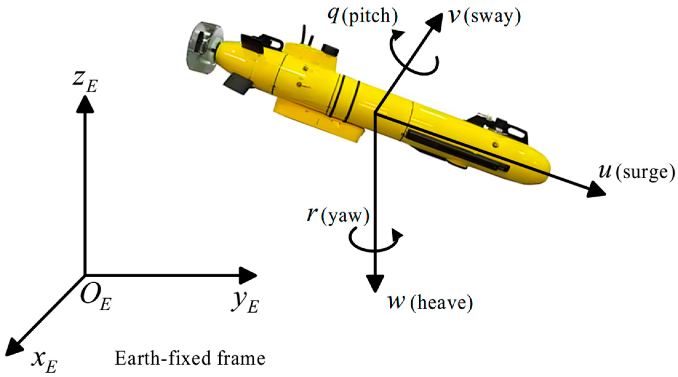
This study investigates the five-degree-of-freedom dynamic model of autonomous underwater vehicles in an inertial reference frame. The main symbols of this article are listed in the

Table A1. Main symbols of this article.

Symbol	Definition	Symbol	Definition
$M_{ud}$	The inertia matrix of underactuated AUVs	$C_{ud}$	The Coriolis-centripetal matrix of underactuated AUVs
$D_{ud}$	The hydrodynamic damping matrix of underactuated AUVs	$G_{ud}$	The restoring force vector of underactuated AUVs
${\tau }_{ud}$	The input of underactuated AUVs	${\tau }_{dis}$	The disturbances of underactuated AUVs
${\delta }_i$	The desired formation vector	$x_0$	The position of virtual leader AUVs
$v_0$	The velocity of virtual leader AUVs	$x_i$	The position of virtual follower AUVs
$v_i$	The velocity of virtual follower AUVs	$v_i^o$	The virtual velocity of virtual follower AUVs
$e_i$	$\mathrm{The} \mathrm{error} \mathrm{between} v_i$$\mathrm{and} v_i^o$	$k_1,\dots ,k_6$	The parameters to be designed in the CFTG Layer controllers
$\alpha ,\beta ,\gamma ,\varsigma$	The parameters to be designed in the CFTG Layer controllers	$\mu ,g,c$	The parameters to be designed in the APF method
${\eta }_{CL}$	The desired trajectory of actual AUVs	${\eta }_1$	The position of actual AUVs
${\nu }_{ud}$	The velocity of actual AUVs	${\nu }^{\ast }$	The virtual velocity of actual AUVs
$e_v$	$\mathrm{The} \mathrm{error} \mathrm{between} {\nu }_{ud}$$\mathrm{and} {\nu }^{\ast }$	$h_1,\dots ,h_6$	The parameters to be designed in the ATT Layer controllers
$\theta ,\sigma ,\xi ,\zeta$	The parameters to be designed in the ATT Layer controllers

which can be found in Appendix A. To enhance the practical relevance of the proposed control framework and directly address platform applicability, we based our analysis on a representative underactuated AUV with specifications comparable to widely used models such as the REMUS-100. The vehicle was equipped with a 1080p HD camera operating at 30 frames per second, enabling effective medium-resolution underwater imaging and object recognition. It supported operational depths of up to 100 m, consistent with common mission scenarios such as seabed mapping and underwater infrastructure inspection. Furthermore, the platform was capable of operating in sea conditions up to Sea State 3 (wave height of 0.5–1.25 m). Figure 1 depicts the three-dimensional configuration of AUVs.

The kinematic and dynamic equations are formulated as:

$$\begin{array}{l}\dot{\eta }=J(\eta )\nu \\ M\dot{\nu }+C(\nu )\nu +D(\nu )\nu +G(\eta )=\tau +{\varpi }_{dis}\end{array}$$

(1)

where $\eta ={[{\eta }_1,{\eta }_2]}^T$, and the position vector ${\eta }_1={[x,y,z]}^T$ and attitude vector ${\eta }_2={[\theta ,\psi ]}^T$, respectively, describe the spatial coordinates and orientation in the earth-fixed frame. The body-fixed frame velocities $\nu ={[{\nu }_1,{\nu }_2]}^T$ are represented by the linear velocity vector ${\nu }_1={[u,v,w]}^T$ and angular velocity vector ${\nu }_2={[q,r]}^T$. The coordinate transformation matrix $J(\eta )=[J_1,0_{3\times 2};0_{2\times 3},J_2]\in {ℝ}^{5\times 5}$ facilitates parameter conversion between reference frames. The system inertia matrix $M\in {ℝ}^{5\times 5}$ incorporates mass and hydrodynamic added-mass effects, while the Coriolis-centripetal matrix $C(\nu )\in {ℝ}^{5\times 5}$ accounts for frame rotation dynamics. The hydrodynamic damping matrix $D(\nu )\in {ℝ}^{5\times 5}$ characterizes viscous drag forces, and the restoring force vector $G(\eta )\in {ℝ}^5$ comprises buoyancy and gravitational effects. The control input vector $\tau$ and environmental disturbance vector ${\varpi }_{dis}\in {ℝ}^5$ represent actuator forces/moments and exogenous perturbations, respectively.

Through actuation analysis, the system can be decoupled into fully actuated and underactuated subsystems. Following the underactuated modeling framework [28], the subsystem dynamics are expressed as:

$$M_{ud}{\dot{\nu }}_{ud}+C_{ud}{\nu }_{ud}+D_{ud}{\nu }_{ud}+G_{ud}={\tau }_{ud}+{\tau }_{dis}$$

(2)

where $M_{ud}\in {ℝ}^{3\times 3}$, $C_{ud}\in {ℝ}^{3\times 3}$, $D_{ud}\in {ℝ}^{3\times 3}$, $G_{ud}\in {ℝ}^3$, ${\tau }_{dis}\in {ℝ}^3$, ${\nu }_{ud}={[u,q,r]}^T$, and ${\tau }_{ud}={[{\tau }_u,{\tau }_q,{\tau }_r]}^T$. When the initial deviation of the system state is large, the computed control torque may exceed the normal operating range of the actuator and enter the saturation zone, which can degrade the control performance. Input saturation arises from two primary factors: the inherent saturation limit of the actuator itself and the presence of the integral term in the control architecture. To address this problem, the saturated input is defined as follows:

$${\tau }_{ud}=sat({\tau }_c)=\left\{\begin{array}{cc}A\cdot \mathrm{sign}({\tau }_c)\hfill & \hfill , \left|{\tau }_c\right|>A\\ {\tau }_c\hfill & \hfill , \left|{\tau }_c\right|\le A\end{array}\right.$$

(3)

where $sat({\tau }_c)$ represents the saturated input nonlinearity function related to the control input ${\tau }_c$, and $A$ is the bound of ${\tau }_c$.

Subsequently, it can be deduced that

$$\mathrm{\Delta }\tau ={\tau }_{ud}-{\tau }_c$$

(4)

Furthermore, the underactuated AUVs based on above model have the following relevant properties [28].

Property 1: The time derivative of $J_1$ can be expressed by a skew-symmetric matrix $P$:

$${\dot{J}}_1=J_{1}P$$

(5)

where $P=\left[\begin{array}{ccc}0& -r& q\\ r& 0& 0\\ -q& 0& 0\end{array}\right]$. Hence, for any vector $m\in {ℝ}^3$, it satisfies $m^{T}Pm=0$.

Property 2: In the underactuated AUV model, the norms of matrices $M_{ud}$, $C_{ud}$, $D_{ud}$, $G_{ud}$, and ${\tau }_{dis}$ satisfy the following inequalities:

$$m_1\le ‖M_{ud}‖\le m_2,‖C_{ud}‖\le c‖{\nu }_{ud}‖,‖D_{ud}‖\le d_1+d_2‖{\nu }_{ud}‖,‖G_{ud}‖\le g,‖{\tau }_{dis}‖\le \widehat{\tau }$$

(6)

where $m_1$, $m_2$, $c$, $d_1$, $d_2$, $g$, and $\widehat{\tau }$ are unknown positive constants.

The objective is to construct the hierarchical architecture to solve the multiple underactuated AUV formation problem and design corresponding control protocols at each layer to ensure that each layer achieves its respective goals. Then, the multi-AUV can achieve formation within a fixed time, i.e.,

$$\underset{t\to T_{\max }}{\lim }‖{\eta }_i-{\eta }_0+{\delta }_i‖=0$$

(7)

where ${\eta }_0$ denotes the state of the leader and ${\delta }_i$ is the desired formation vector.

2.2. Graph Theory

Within the leader–follower network system architecture, the multiagent communication topology among follower agents can be modeled as an undirected graph $G=\left\{\upsilon ,\phi ,A\right\}$, where $\upsilon =\left\{{\nu }_1,{\nu }_2,\dots ,{\nu }_N\right\}$ denotes the node set and $\phi \subseteq \left\{\left\{m,n\right\}\left|m,n\in \upsilon ,m\ne n\right.\right\}$ represents the bidirectional edge set. An edge $e_{mn}\in \phi$ exists if and only if mutual information exchange occurs between follower $m$ and follower $n$. The topological structure is mathematically encoded through an adjacency matrix $A=(a_{mn})\in {ℝ}^{N\times N}$, where $a_{mn}=1$ for $e_{mn}\in \phi$ and $a_{mn}=0$ otherwise. Notably, self-connections are excluded from the topology ($a_{mm}=0$). The Laplacian matrix $\mathcal{L}=(l_{mn})\in {ℝ}^{N\times N}$ is constructed with diagonal entries $l_{mn}={\displaystyle {\sum }_{m=1,m\ne n}^N{a}_{mn}}$ and off-diagonal elements $l_{mn}=-a_{mn},m\ne n$. Furthermore, the leader–follower interaction topology is characterized by matrix $B=diag\{b_1,b_2,\dots ,b_N\}$, where $b_m=1$ indicates direct state transmission from leaders to follower $m$, while $b_m=0$ signifies the absence of immediate leader-to-follower communication channels.

2.3. Lemmas

Lemma 1

[29]. Suppose $x\in {ℝ}^n$ and $V(\cdot ):{ℝ}^n\to {ℝ}_{+}\cup \left\{0\right\}$ is a continuous, positive definite, and radially unbounded function; then, the two following conditions hold:

(1) 

$V(x(t))=0\iff x(t)=0$.

(2) 

The function $V(x(t))$ satisfies

• $\dot{V}(x(t))\le -a_1{V}^{\alpha }(x(t))-a_2{V}^{\beta }(x(t))-a_{3}V(x(t))$

where  $a_1,a_2,a_3>0, 0<\alpha <1$ and $\beta >1$  are all constants. Then,  $x(t)=0$ is a fixed-time stable equilibrium point, and the settling time is calculated as:

$$T\le T_{\max }=\frac{1}{a_3(1-\alpha )}\ln (1+\frac{a_3}{a_1})+\frac{1}{a_3(\beta -1)}\ln (1+\frac{a_3}{a_2})$$

(8)

Lemma 2

[30]. Assume that ${\gamma }_1,{\gamma }_2,\dots {\gamma }_N\ge 0$. Then,

$$\begin{array}{l}{\displaystyle \sum _{i=1}^N{\gamma }_i^d}\ge {({\displaystyle \sum _{i=1}^N{\gamma }_i})}^d,d\in \left(0,1\right]\\ {\displaystyle \sum _{i=1}^N{\gamma }_i^d}\ge N^{1-d}{({\displaystyle \sum _{i=1}^N{\gamma }_i})}^d,d\in \left(1,\infty \right)\end{array}$$

(9)

Lemma 3

[31]. Let $x\in {ℝ}^n$ and define$\mathrm{sig}{(x)}^{\gamma }={\left[\mathrm{sign}(x_1){\left|x_1\right|}^{\gamma },\dots ,\mathrm{sign}(x_n){\left|x_n\right|}^{\gamma }\right]}^T$. Then, for each component, we have

$$\begin{array}{l}\frac{d}{dx}{\left|x\right|}^{\gamma +1}=(\gamma +1)\mathrm{sig}{(x)}^{\gamma }\\ \frac{d}{dx}\mathrm{sig}{(x)}^{\gamma +1}=(\gamma +1){\left|x\right|}^{\gamma }\end{array}$$

(10)

3. Hierarchical Architecture of Formation Control for Multiple Underactuated AUVs

This section described the hierarchical control architecture specifically designed for the formation regulation of multiple underactuated autonomous underwater vehicles. Under the proposed architecture, the trajectories generation and trajectories tracking controllers are designed separately, which significantly improves the flexibility and practicality of the system. Furthermore, it provides a possibility that a new AUV or other autonomous intelligent platform can join into the formation tasks without changing their origin control strategy, which significantly improves the adaptability and expandability of the system.

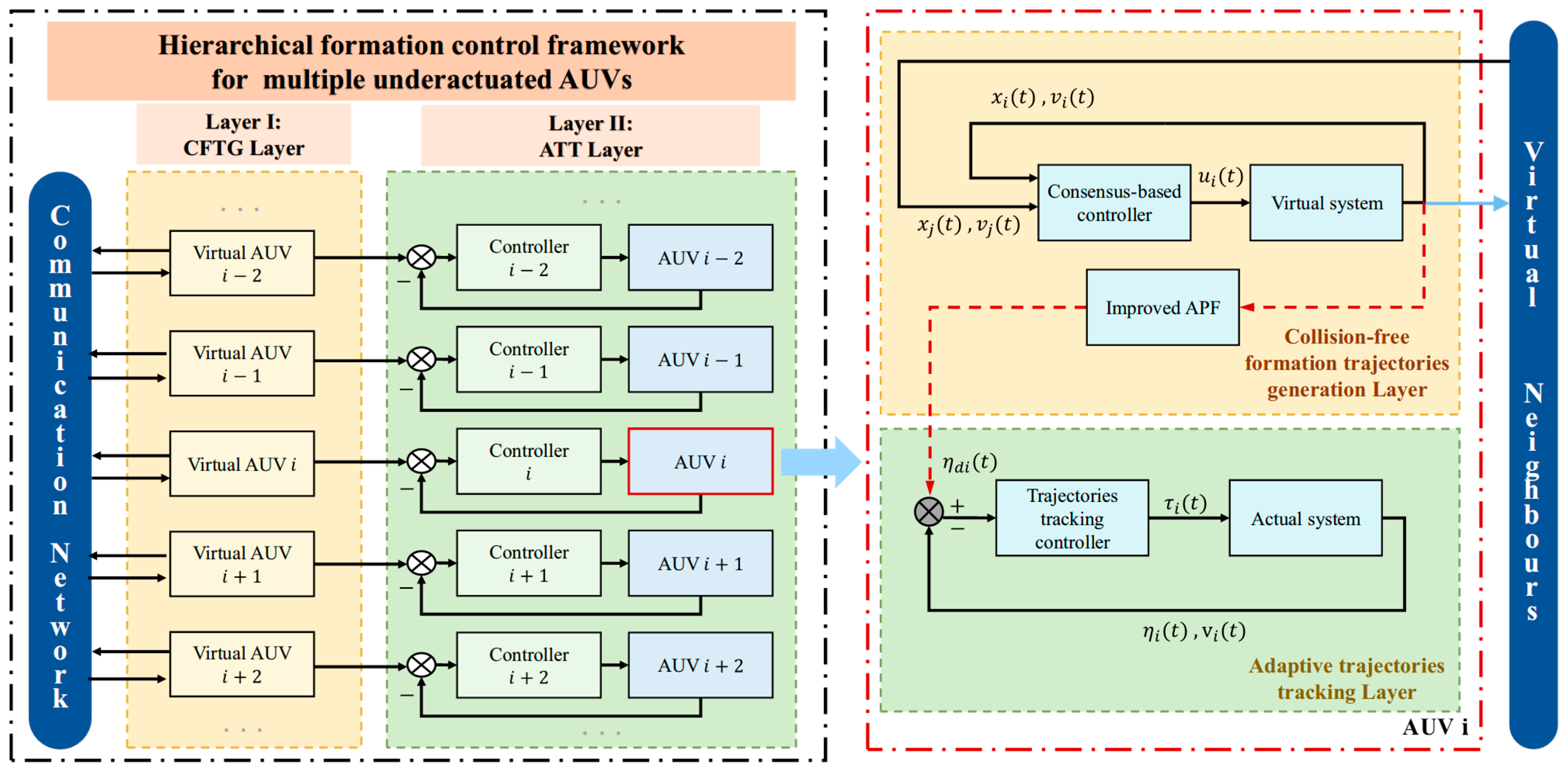
The architecture of the hierarchical framework for multiple underactuated AUVs’ formation control is depicted in Figure 2. Compared with the current AUVs’ formation control methods, the hierarchical framework does not calculate formation errors and send it to AUVs’ individual controller directly as a swarm reference signal. Instead, the proposed architecture systematically decouples the formation maintenance objectives and individual AUV dynamics control through a dual-layer structure comprising: the Collision-free Formation Trajectories Generation Layer (CFTG Layer) and the Adaptive Trajectories Tracking Layer (ATT Layer).

The CFTG Layer acts as virtual AUV nodes, generating desired trajectories for AUVs that meet the requirement of complex formation tasks. The ATT Layer tracks the desired trajectories using the control protocols designed based on the kinematic and dynamic models of AUV. Both the desired trajectory and the sensors’ signals are the input of the trajectory tracking controller, which guarantee AUVs can track the desired trajectories precisely and complete the tasks.

The formation control strategy for each AUV is divided into two components: trajectory generation and trajectory tracking. The reference trajectory, generated by a fixed-time consensus controller combined with an enhanced artificial potential field (APF) method, serves as an input to the fixed-time trajectory tracking controller. By integrating this reference trajectory with real-time sensor data, the AUV can accurately follow the prescribed trajectory under the guidance of the tracking controller, thereby fulfilling its designated role in the formation. While both control layers rely on signals detected and processed by the AUV, their interaction does not involve direct communication but rather shared signal utilization across the hierarchical framework.

Compared to existing AUV formation control strategies, the hierarchical framework offers several advantages: (1) Decoupled Design: By separating swarm-level coordination (e.g., consensus or formation shape maintenance) from individual-level trajectory tracking, controllers at each layer can be independently optimized for specific objectives. This modularity enhances flexibility and simplifies integration into diverse operational scenarios. (2) Reduced Interdependence: Swarm behaviors and individual AUV dynamics are decoupled, eliminating mutual constraints. Consequently, new AUVs or even heterogeneous autonomous platforms can join the formation without modifying their native control architectures, improving adaptability and scalability.

4. Collision-Free Formation Trajectories Generation Layer Design

In this section, the design of the CFTG Layer is introduced. After obtaining the initial states by sensors, virtual AUVs communicate over a distributed network. A fixed-time consensus-based controller is proposed to meet the desired formation requirements. Meanwhile, an enhanced artificial potential field methodology is developed to achieve obstacle avoidance. The systems generate reference states, which are then used to form the desired trajectories for the ATT Layer.

In the CFTG Layer, the system of virtual AUV is considered as a second-order model for the following reasons:

(1) To mitigate the impact of underactuated AUVs’ complex dynamic and kinematic characteristics on trajectory generation controller design for formation missions.

(2) To ensure the generated trajectories can be tracked by actual underactuated AUVs.

The virtual leader’s model in the CFTG Layer is defined as:

$$\begin{array}{l}{\dot{x}}_0=v_0\\ {\dot{v}}_0=u_0+f_0(x_0,v_0)\end{array}$$

(11)

where $x_0={\eta }_0$, $v_0={\nu }_0$, and $‖f_0(x_0,v_0)‖\le F_0$, $F_0$ is a positive constant.

The virtual follower’s model in the CFTG Layer is defined as:

$$\begin{array}{l}{\dot{x}}_i=v_i\\ {\dot{v}}_i=u_i+f_i(x_i,v_i)\end{array}$$

(12)

where $x_i={\eta }_i$, $v_i={\nu }_i$, $‖f_i(x_i,v_i)‖\le F_i$, and $F_i$ is a positive constant.

4.1. Backstepping-Based Fixed-Time Consensus Control Protocol Design

Based on backstepping control methods, the design of fixed-time consensus control protocols in the CFTG Layer can be divided into two steps:

(1) Design the virtual velocity $v_i^o$ to let $x_i$ reach consensus and maintain formation within a fixed time.

(2) Design the input $u_i$ to let the true velocity $v_i$ track the virtual velocity $v_i^o$ within a fixed time.

To express the formation characteristic, define ${\widehat{x}}_i=x_i+{\delta }_i$, ${\tilde{x}}_i={\widehat{x}}_i-x_0$.

The virtual velocity $v_i^o$ is designed as follows:

$$\begin{array}{ll}{v}_i^o=& -k_1\mathrm{sig}{({\displaystyle \sum _{j=1}^N{a}_{ij}({\widehat{x}}_i-{\widehat{x}}_j)+b_i{\tilde{x}}_i})}^{\alpha }-k_2\mathrm{sig}{({\displaystyle \sum _{j=1}^N{a}_{ij}({\widehat{x}}_i-{\widehat{x}}_j)+b_i{\tilde{x}}_i})}^{\beta }\\ & -k_3\mathrm{sig}({\displaystyle \sum _{j=1}^N{a}_{ij}({\widehat{x}}_i-{\widehat{x}}_j)+b_i{\tilde{x}}_i})\end{array}$$

(13)

where $k_1$, $k_2$, and $k_3$ are positive constants and $\alpha \in (0,1)$, $\beta \in (1,\infty )$.

Then, define the error $e_i$ between true velocity $v_i$ and virtual velocity $v_i^o$ for each AUV:

$$e_i=v_i-v_i^o$$

(14)

Thus, one has that

$$\begin{array}{ll}{\dot{e}}_i=& u_i+f_i(x_i+v_i)+k_1\alpha {\left|{\displaystyle \sum _{j=1}^N{a}_{ij}({\widehat{x}}_i-{\widehat{x}}_j)+b_i{\tilde{x}}_i}\right|}^{\alpha -1}({\displaystyle \sum _{j=1}^N{a}_{ij}(v_i-v_j)+b_i{\tilde{v}}_i})\\ & +k_2\beta {\left|{\displaystyle \sum _{j=1}^N{a}_{ij}({\widehat{x}}_i-{\widehat{x}}_j)+b_i{\tilde{x}}_i}\right|}^{\beta -1}({\displaystyle \sum _{j=1}^N{a}_{ij}(v_i-v_j)+b_i{\tilde{v}}_i})+k_3({\displaystyle \sum _{j=1}^N{a}_{ij}(v_i-v_j)+b_i{\tilde{v}}_i})\end{array}$$

(15)

The control input $u_i$ is designed as:

$$\begin{array}{ll}{u}_i=& -k_1\alpha {\left|{\displaystyle \sum _{j=1}^N{a}_{ij}({\widehat{x}}_i-{\widehat{x}}_j)+b_i{\tilde{x}}_i}\right|}^{\alpha -1}({\displaystyle \sum _{j=1}^N{a}_{ij}(v_i-v_j+b_i{\tilde{v}}_i})\\ & -k_2\beta {\left|{\displaystyle \sum _{j=1}^N{a}_{ij}({\widehat{x}}_i-{\widehat{x}}_j)+b_i{\tilde{x}}_i}\right|}^{\beta -1}({\displaystyle \sum _{j=1}^N{a}_{ij}(v_i-v_j)+b_i{\widehat{v}}_i})\\ & -k_3({\displaystyle \sum _{j=1}^N{a}_{ij}(v_i-v_j)+b_i{\tilde{v}}_i})-k_4\mathrm{sig}{(e_i)}^{\gamma }-k_5\mathrm{sig}{(e_i)}^{\varsigma }-k_6\mathrm{sig}(e_i)-F_i\mathrm{sign}(e_i)\end{array}$$

(16)

where $k_4$, $k_5$, and $k_6$ are positive constants and $\gamma \in (0,1)$,$\varsigma \in (1,\infty )$.

Theorem 1.

Consider the leader–follower multiple virtual AUVs (12) under controller (16). The virtual AUVs (12) can reach consensus and maintain formation within a fixed time. Thus, the CFTG Layer is capable of calculating virtual states and generating reference trajectories for AUVs within a fixed time.

Proof. 

(1) To verify that the true velocity can track the virtual velocity within a fixed time, we chose the Lyapunov function as follows:

$$V_1=\frac{1}{2}{\displaystyle \sum _{i=1}^N{e}_i^2}$$

(17)

Then, the derivative of $V_1$ can be calculated as:

$$\begin{array}{ll}{\dot{V}}_1& ={\displaystyle \sum _{i=1}^N{e}_i}{\dot{e}}_i\\ & ={\displaystyle \sum _{i=1}^N(-k_4{e}_i\mathrm{sig}{(e_i)}^{\gamma }-k_5{e}_i\mathrm{sig}{(e_i)}^{\varsigma }-k_6{e}_i\mathrm{sig}(e_i)+e_i{f}_i(x_i,v_i)-e_i{F}_i\mathrm{sign}(e_i))}\\ & \le -k_4{\displaystyle \sum _{i=1}^N{\left|e_i\right|}^{\gamma +1}}-k_5{\displaystyle \sum _{i=1}^N{\left|e_i\right|}^{\varsigma +1}}-k_6{\displaystyle \sum _{i=1}^N{\left|e_i\right|}^2}\end{array}$$

(18)

According to Lemma 2, one has that

$$\begin{array}{ll}{\dot{V}}_1& \le -k_4{2}^{\frac{\gamma +1}{2}}{\displaystyle \sum _{i=1}^N{(e_i^2)}^{\frac{\gamma +1}{2}}}-k_5{2}^{\frac{\varsigma +1}{2}}{N}^{\frac{1-\varsigma }{2}}{\displaystyle \sum _{i=1}^N{(e_i^2)}^{\frac{\varsigma +1}{2}}}-k_6{\displaystyle \sum _{i=1}^N(e_i^2)}\\ & \le -k_4{2}^{\frac{\gamma +1}{2}}{V}_1^{\frac{\gamma +1}{2}}-k_5{2}^{\frac{\varsigma +1}{2}}{N}^{\frac{1-\varsigma }{2}}{V}_1^{\frac{\varsigma +1}{2}}-2k_6{V}_1\end{array}$$

(19)

Based on Lemma 1, the settling time can be calculated as:

$$T_1\le T_{1\max }=\frac{1}{p_3(1-\gamma )}\ln (1+\frac{p_3}{p_1})+\frac{1}{p_3(\varsigma -1)}\ln (1+\frac{p_3}{p_2})$$

(20)

where $p_1=k_4{2}^{\frac{\gamma +1}{2}}$, $p_2=k_5{2}^{\frac{\varsigma +1}{2}}{N}^{\frac{1-\varsigma }{2}}$, and $p_3=2k_6$.

Thus, for virtual AUVs in the CFTG Layer, the true velocity can track the virtual velocity within a fixed time.

Remark 1.

It is worth noting that the range of the parameters in the convergence time formula have been specified when they are first introduced. And these parameters are typically treated as design constants and can be adjusted or tuned based on specific system requirements and performance objectives. This flexibility allows the method to be adapted to a variety of scenarios while preserving the theoretical guarantees.

(2) To verify that the system can reach consensus and meet the desired formation requirements within a fixed time, we chose the Lyapunov function as follows:

$$V_2=\frac{1}{2}{\tilde{x}}^T(L+B)\tilde{x}$$

(21)

where $L$ is the Laplacian matrix that describe the topology between followers and $B$ is the matrix that indicate the leader–follower interaction. Based on the definition at the beginning of this part, it can be deduced that ${\tilde{x}}_i=x_i+{\delta }_i-x_0$. To simplify the notation, define ${\widehat{y}}_i={\displaystyle \sum _{j=1}^N{a}_{ij}({\widehat{x}}_i-{\widehat{x}}_j)+b_i{\tilde{x}}_i}$

Then, the derivative of $V_2$ can be calculated as:

$$\begin{array}{ll}{\dot{V}}_2& ={\tilde{x}}^T(L+B)\dot{\tilde{x}}\\ & ={\displaystyle \sum _{j=1}^N{\widehat{y}}_i(v_i-v_0)}\\ & ={\displaystyle \sum _{j=1}^N{\widehat{y}}_i(e_i+v_i^o-v_0)}\\ & ={\displaystyle \sum _{j=1}^N{\widehat{y}}_i(-k_1\mathrm{sig}{({\widehat{y}}_i)}^{\gamma }-k_2\mathrm{sig}{({\widehat{y}}_i)}^{\varsigma }-k_3\mathrm{sig}({\widehat{y}}_i))}\\ & \le -k_1{\displaystyle \sum _{j=1}^N{({\widehat{y}}_i^2)}^{\frac{\gamma +1}{2}}}-k_2{\displaystyle \sum _{j=1}^N{({\widehat{y}}_i^2)}^{\frac{\varsigma +1}{2}}}-k_3{\displaystyle \sum _{j=1}^N{\widehat{y}}_i^2}\\ & \le -k_1{2}^{\frac{\gamma +1}{2}}{V}_2^{\frac{\gamma +1}{2}}-k_2{2}^{\frac{\varsigma +1}{2}}{N}^{\frac{1-\varsigma }{2}}{V}_2^{\frac{\varsigma +1}{2}}-2k_3{V}_2\end{array}$$

(22)

The settling time can be calculated as:

$$T_2\le T_{2\max }=\frac{1}{p_6(1-\gamma )}\ln (1+\frac{p_6}{p_4})+\frac{1}{p_6(\varsigma -1)}\ln (1+\frac{p_6}{p_5})$$

(23)

where $p_4=k_1{2}^{\frac{\gamma +1}{2}}$, $p_5=k_2{2}^{\frac{\varsigma +1}{2}}{N}^{\frac{1-\varsigma }{2}}$, and $p_6=2k_3$.

Remark 2.

It is worth noting that Equation (22) holds for $t>T_1$, where the tracking error $e_i=0$, indicating that the system has entered the convergence phase.

To prove the global stability of virtual AUVs, we chose the Lyapunov function as follows:

$$V=V_1+V_2$$

(24)

Based on the above analysis, the derivative of $V$ can be calculated as:

$$\begin{array}{ll}\dot{V}& \le -k_4{2}^{\frac{\gamma +1}{2}}{\displaystyle \sum _{i=1}^N{(e_i^2)}^{\frac{\gamma +1}{2}}}-k_5{2}^{\frac{\varsigma +1}{2}}{N}^{\frac{1-\varsigma }{2}}{\displaystyle \sum _{i=1}^N{(e_i^2)}^{\frac{\varsigma +1}{2}}}-k_6{\displaystyle \sum _{i=1}^N(e_i^2)}\\ & -k_1{\displaystyle \sum _{j=1}^N{({\widehat{y}}_i^2)}^{\frac{\gamma +1}{2}}}-k_2{\displaystyle \sum _{j=1}^N{({\widehat{y}}_i^2)}^{\frac{\varsigma +1}{2}}}-k_3{\displaystyle \sum _{j=1}^N{\widehat{y}}_i^2}\\ & \le -k_4{2}^{\frac{\gamma +1}{2}}{V}_1^{\frac{\gamma +1}{2}}-k_5{2}^{\frac{\varsigma +1}{2}}{N}^{\frac{1-\varsigma }{2}}{V}_1^{\frac{\varsigma +1}{2}}-2k_6{V}_1\\ & -k_1{2}^{\frac{\gamma +1}{2}}{V}_2^{\frac{\gamma +1}{2}}-k_2{2}^{\frac{\varsigma +1}{2}}{N}^{\frac{1-\varsigma }{2}}{V}_2^{\frac{\varsigma +1}{2}}-2k_3{V}_2\\ & \le -\min \left\{k_1,k_4\right\}{2}^{\frac{\gamma +1}{2}}{V}^{\frac{\gamma +1}{2}}-\min \left\{k_2,k_5\right\}{2}^{\frac{\varsigma +1}{2}}{N}^{\frac{1-\varsigma }{2}}{V}^{\frac{\varsigma +1}{2}}-\min \left\{k_3,k_6\right\}V\end{array}$$

(25)

Remark 3.

The proposed backstepping-based control design ensures that the closed-loop system is forward-complete and free from finite-time escape. This property follows from the recursive construction of Lyapunov functions in each step of the backstepping procedure, where the control inputs are continuously designed and the error dynamics are stabilized incrementally.

Hence, in the CFTG Layer, both the system’s velocity and positions can achieve convergence and the reference trajectories composed of virtual states can be generated within settling time $T_{CFTG}=T_{1\max }+T_{2\max }$. The proof is complete. □

4.2. Improved Artificial Potential Field Method Design

While the precomputed formation trajectory provides nominal navigation paths for the multi AUVs, real-world marine environments often contain static and dynamic obstacles requiring reactive collision avoidance. The artificial potential field method can solve this problem by dynamically modifying the planned trajectories through the superposition of virtual force fields.

However, a fundamental limitation in conventional artificial potential field methods arises when targets are positioned near obstacles, creating conflicting gradient interactions. The attractive potential drives the AUV toward the target, while proximity to obstacles induces repulsive forces. When the magnitude of repulsion surpasses attraction, the AUV cannot reach the target. Thus, we introduced an improved artificial potential field method to address the problem of the target being unreachable. The distance between the AUV and its target is added to the repulsive potential function, which is used to change the repulsive force influence of obstacles near the target point.

In the CFTG Layer, the calculated position state at the next moment can be regarded as the target point. Let $x_g$ represent the position of the target point. Then, the attractive potential function is:

$$U_{att}(x)=\frac{k}{2}{d}^2(x,x_g)$$

(26)

where $k$ is the gain coefficient and $d(x,x_g)$ represents the distance between the AUV and the target.

The gravity of the corresponding attractive force is:

$$F_{att}=-\nabla U_{att}=kd(x,x_g)$$

(27)

Let $x_o$ represent the position of the center of the obstacle. Then, the improved repulsive potential function can be expressed as:

$$U_{rep}(x)=\left\{\begin{array}{cc}\frac{\mu }{e^{\frac{d(x,x_o)}{c}}-e^{\frac{d_{\min }(x,x_o)}{c}}}\cdot \frac{d^2(x,x_g)}{g}\hfill & , d(x,x_o)\le R\hfill \\ 0\hfill & , else\hfill \end{array}\right.$$

(28)

where $\mu$, $c$, and $g$ are gain coefficients; $R$ represents the influence radius of obstacles; $d_{\min }(x,x_o)$ is the minimum value of $d(x,x_o)$; $d(x,x_o)$ represents the distance between the AUV and obstacles; and $d(x,x_g)$ is the distance between the AUV and the target.

The corresponding repulsive force is:

$$F_{rep}=\left\{\begin{array}{cc}\frac{\mu }{c}\cdot \frac{e^{\frac{d(x,x_o)}{c}}}{{(e^{\frac{d(x,x_o)}{c}}-e^{\frac{d_{\min }(x,x_o)}{c}})}^2}\cdot \frac{d^2(x,x_g)}{g}\hfill & \\ \_\frac{\mu }{g}\cdot \frac{d(x,x_g)}{e^{\frac{d(x,x_o)}{c}}-e^{\frac{d_{\min }(x,x_o)}{c}}}\hfill & , d(x,x_o)\le R\hfill \\ 0\hfill & , else\hfill \end{array}\right.$$

(29)

Thus, the resultant force acting on the AUV is:

$$F_{res}=F_{att}+F_{rep}$$

(30)

When the obstacles are near the precomputed formation trajectory ($d(x,x_o)\le R$), the AUV is influenced by resultant force $F_{res}$. With this force, the AUV dynamically avoids obstacles while simultaneously progressing toward the target configuration. When the AUV comes closer to target, $d(x,x_g)$ converges to zero, which means $F_{rep}$ also converges to zero. Thus, the problem in conventional AFD methods that the AUV cannot reach the target when the target is close to obstacles can be solved.

Remark 4.

The improved artificial potential field method in our framework plays a modular role in enhancing obstacle avoidance without interfering with the stability guarantees of the control system. In the first layer of the control architecture, a desired trajectory $x_i$ is generated based on formation and task objectives, without considering obstacle information. This trajectory may intersect with static obstacles in the environment. To address this, the APF method is applied as a trajectory modification module that locally adjusts $x_i$ to produce a new, collision-free reference trajectory ${\eta }_{CL}$. This updated trajectory serves as the desired trajectory for the actual AUVs. The relationship between the virtual state $x_i$ and the collision-free reference trajectory ${\eta }_{CL}$ is summarized by the following equation: ${\eta }_{CL}(t)=x_i(t)+\mathrm{\Delta }t\cdot F_{res}$, where $\mathrm{\Delta }t$ is the step size and $F_{res}$ is the resultant force. In the second layer, the controller is designed to ensure that the AUV tracks ${\eta }_{CL}$ within a fixed time. Since this layer treats ${\eta }_{CL}$ as a known and continuously updated reference, the control design remains independent of the internal workings of the APF. As a result, the Lyapunov-based stability and fixed-time convergence analyses are still valid, as they are performed relative to the updated reference trajectory. This layered structure enables safe and flexible operation without compromising theoretical rigor.

5. Adaptive Trajectories Tracking Layer Design

In this section, the design of ATT Layer is presented. In the ATT Layer, each AUV can precisely track the trajectories generated by the CFTG Layer. Based on the auxiliary compensation system, we propose an adaptive fixed-time trajectories tracking method for underactuated AUVs subject to uncertain disturbances and saturated inputs.

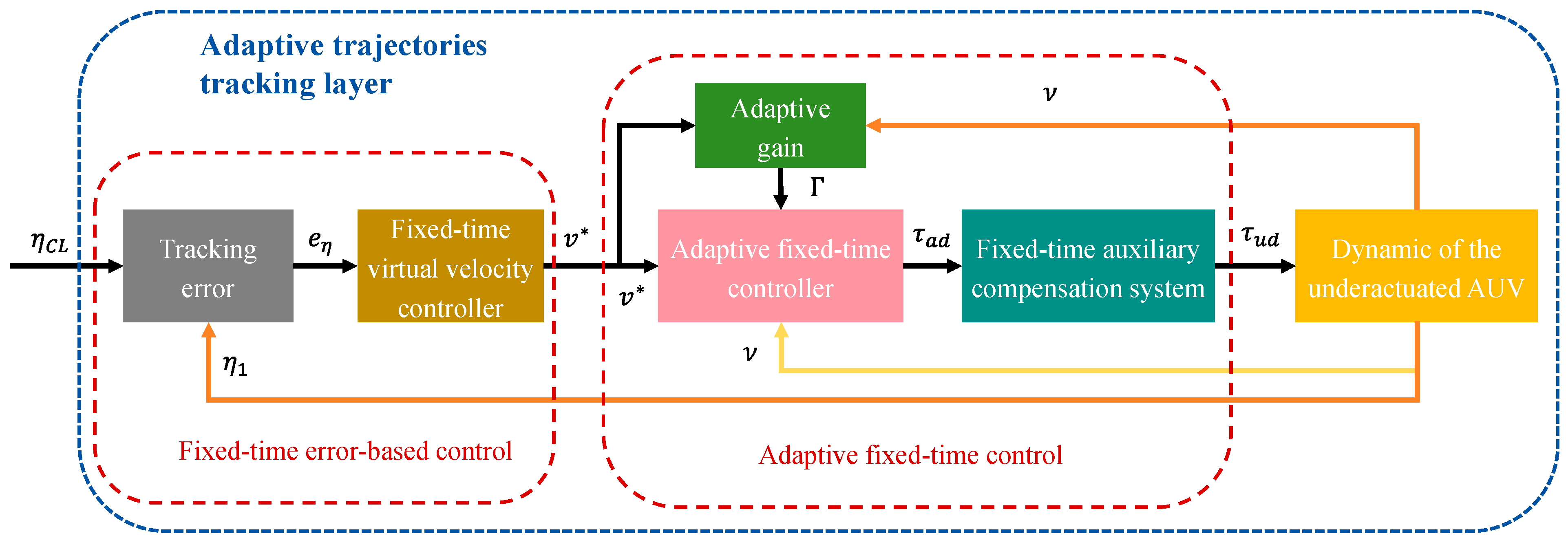
Figure 3 shows the block diagram of Adaptive Trajectories Tracking Layer. Based on the backstepping method, the trajectory tracking controller takes both the desired trajectory and sensor signals as inputs. The error between them is defined as the tracking error, which serves as the input to the fixed-time virtual velocity control law. An adaptive fixed-time control law is proposed to overcome the unknown parameters in underactuated AUVs’ models and external disturbances. Moreover, a fixed-time auxiliary compensation system is constructed to address the influence of saturated inputs. Under designed controllers, each AUV can track the desired trajectories generated by the CFTG Layer within a fixed time.

For a single underactuated AUV, let ${\eta }_{CL}$ be the desired trajectory. Then, the tracking error can be represented as follows:

$${\eta }_e={\eta }_1-{\eta }_{CL}$$

(31)

Subsequently, the trajectory tracking error in body-fixed frame is deduced as:

$$e_{\eta }=J_1^T{\eta }_e$$

(32)

If $e_{\eta }=0$, then ${\eta }_e=0$. Hence, the trajectory tracking problem is transformed into how can $e_{\eta }$ achieve convergence within a fixed time.

Based on Equations (5) and (32), the derivative of $e_{\eta }$ is

$$\begin{array}{ll}{\dot{e}}_{\eta }& ={\dot{J}}_1^T{\eta }_e+J_1^T(J_1{\nu }_1-{\dot{\eta }}_{CL})\\ & =P^T{J}_1^T{\eta }_e+J_1^T{J}_1{\nu }_1-J_1^T{\dot{\eta }}_{CL}\\ & =-P{e}_{\eta }+{\nu }_{ud}+{[0,v-q,w-r]}^T-J_1^T{\dot{\eta }}_{CL}\end{array}$$

(33)

Define the virtual velocity control protocol as ${\nu }^{\ast }={[u^{\ast },q^{\ast },r^{\ast }]}^T$ and the velocity error as $e_v={\nu }_{ud}-{\nu }^{\ast }$. Thus, the derivative of $e_{\eta }$ can be rewritten as:

$${\dot{e}}_{\eta }=-P{e}_{\eta }+{\nu }^{\ast }+e_v+{[0,v-q,w-r]}^T-J_1^T{\dot{\eta }}_{CL}$$

(34)

Similar to the CFTG Layer, based on backstepping method, the virtual velocity control protocol is designed as:

$${\nu }^{\ast }=J_1^T{\dot{\eta }}_{CL}-h_1\mathrm{sig}{(e_{\eta })}^{\theta }-h_2\mathrm{sig}{(e_{\eta })}^{\sigma }-h_3\mathrm{sig}(e_{\eta })-{[0,v-q,w-r]}^T$$

(35)

where $h_1$, $h_2$, and $h_3$ are positive constants and $\theta \in (0,1)$,$\sigma \in (1,\infty )$.

To address the saturated inputs, we propose a fixed-time auxiliary compensation system as follows:

$$\dot{\phi }=\left\{\begin{array}{cc}-l_1\mathrm{sig}{(\phi +\mathrm{\Delta }\tau )}^{\xi }-l_2\mathrm{sig}{(\phi +\mathrm{\Delta }\tau )}^{\zeta }-l_3\mathrm{sig}(\phi +\mathrm{\Delta }\tau )-\mathrm{\Delta }\dot{\tau }\hfill & , {‖\phi ‖}_2\ge {\phi }_0\hfill \\ 0\hfill & , else\hfill \end{array}\right.$$

(36)

where ${\phi }_0$ is chosen according to the saturation limits of the actuator, while $l_1$, $l_2$, and $l_3$ are positive constants;$\xi \in (0,1)$ and $\zeta \in (1,\infty )$.

Remark 5.

In our implementation, we defined $\mathrm{\Delta }\tau ={\tau }_{ud}-{\tau }_c$, where ${\tau }_c$ is the ideal control input computed from the controller and ${\tau }_{ud}=sat({\tau }_c)$ is the actual bound input applied to the vehicle after considering input saturation. Since both ${\tau }_c$ and ${\tau }_{ud}$ are available in real time, where ${\tau }_c$ is directly computed from the control law and ${\tau }_{ud}$ is the output of the saturation function, the value of $\mathrm{\Delta }\tau$ can be determined accordingly. Therefore, its derivative $\mathrm{\Delta }\dot{\tau }$ can be approximated numerically using discrete-time methods (e.g., forward difference) without requiring knowledge of the vehicle’s velocity derivatives or system parameters.

Thus, combining with the adaptive control methods, the control input is designed as:

$${\tau }_c=m({\tau }_{ad}+\phi )=m(-h_4\mathrm{sig}{(e_v)}^{\theta }-h_5\mathrm{sig}{(e_v)}^{\sigma }-h_6\mathrm{sig}(e_v)-\mathrm{\Gamma }\mathrm{sig}(e_v)+\phi )$$

(37)

where $m>m_2$; $h_4$, $h_5$, and $h_6$ are positive constants; $\mathrm{\Gamma }={\tilde{g}}_0+{\tilde{g}}_1‖\nu ‖+{\tilde{g}}_2{‖\nu ‖}^2$ is the adaptive gain;, and ${\tilde{g}}_i$ is calculated by the following adaptive equation:

$${\dot{\tilde{g}}}_i=-\mathrm{sig}{({\tilde{g}}_i)}^{\theta }-\mathrm{sig}{({\tilde{g}}_i)}^{\sigma }-\mathrm{sig}({\tilde{g}}_i)$$

(38)

Theorem 2.

Consider the underactuated AUV subject to input saturation (2), under controller (37), $e_{\eta }$ can converge to zero within a fixed time. Thus, in the ATT Layer, each AUV can track the desired trajectories generated by the CFTG Layer, i.e., under the designed hierarchical controllers, multi-AUVs can complete the formation task within a fixed time.

Proof. 

(1) To verify that the velocity error $e_v$ can converge to zero within a fixed time, consider the Lyapunov function as:

$$V_3=\frac{1}{2m}{e}_v^T{M}_{ud}{e}_v$$

(39)

Subsequently, the derivative of $V_3$ is deduced as:

$$\begin{array}{ll}{\dot{V}}_3& =\frac{1}{m}{e}_v^T{M}_{ud}{\dot{e}}_v\\ & =\frac{1}{m}{e}_v^T(M_{ud}{\dot{\nu }}_{ud}-M_{ud}{\dot{\nu }}^{\ast })\\ & =\frac{1}{m}{e}_v^T({\tau }_{ud}-C_{ud}{\nu }_{ud}-D_{ud}{\nu }_{ud}-G_{ud}+{\tau }_{dis}-M_{ud}{\dot{\nu }}^{\ast })\end{array}$$

(40)

Let $G=m^{-1}(-C_{ud}{\nu }_{ud}-D_{ud}{\nu }_{ud}-G_{ud}+{\tau }_{dis}-M_{ud}{\dot{\nu }}^{\ast })$. Based on property 2, $G$ satisfies the following inequality:

$$\begin{array}{ll}‖G‖& \le m^{-1}(c{‖{\nu }_{ud}‖}^2+d_1‖{\nu }_{ud}‖+d_2{‖{\nu }_{ud}‖}^2+g+\widehat{\tau }+m_2‖{\nu }^{\ast }‖)\\ & \le g_0+g_1‖{\nu }_{ud}‖+g_2{‖{\nu }_{ud}‖}^2\end{array}$$

(41)

where $g_0$, $g_1$, and $g_2$ are unknown positive constants related to the parameters of the underactuated AUV models.

Thus, the derivative of $V_3$ can be rewritten as:

$$\begin{array}{ll}{\dot{V}}_3& =e_v^T(\frac{{\tau }_{ud}}{m}+G)\\ & =e_v^T(\frac{{\tau }_c+\mathrm{\Delta }\tau }{m}+G)\\ & =e_v^T(-h_4\mathrm{sig}{(e_v)}^{\theta }-h_5\mathrm{sig}{(e_v)}^{\sigma }-h_6\mathrm{sig}(e_v))-e_v^T\mathrm{\Gamma }+e_v^{T}G+e_v^T(\frac{\phi +\mathrm{\Delta }\tau }{m})\\ & \le e_v^T(-h_4\mathrm{sig}{(e_v)}^{\theta }-h_5\mathrm{sig}{(e_v)}^{\sigma }-h_6\mathrm{sig}(e_v))-e_v^T(‖e_v‖{\displaystyle \sum _{i=0}^2({\tilde{g}}_i-g_i)}{‖{\nu }_{ud}‖}^i)+e_v^T(\frac{\phi +\mathrm{\Delta }\tau }{m})\end{array}$$

(42)

To verify that the designed adaptive control protocols can address the uncertain parameters in the underactuated AUV model and environment disturbances, we chose the Lyapunov function as follows:

$$V_4=\frac{1}{2}{\displaystyle \sum _{i=0}^2{\widehat{g}}_i}$$

(43)

where ${\widehat{g}}_i={\tilde{g}}_i-g_i$ denotes the error between the adaptive parameters and the model parameters. The derivative of $V_4$ is

$$\begin{array}{ll}{\dot{V}}_4& ={\displaystyle \sum _{i=0}^2({\tilde{g}}_i-g_i)}{\dot{\tilde{g}}}_i\\ & =-{\displaystyle \sum _{i=0}^2({\tilde{g}}_i-g_i)}(\mathrm{sig}{({\tilde{g}}_i)}^{\theta }+\mathrm{sig}{({\tilde{g}}_i)}^{\sigma }+\mathrm{sig}({\tilde{g}}_i))\\ & \le -{\displaystyle \sum _{i=0}^2{({\tilde{g}}_i-g_i)}^{\theta +1}}-{\displaystyle \sum _{i=0}^2{({\tilde{g}}_i^i-g_i)}^{\sigma +1}}-{\displaystyle \sum _{i=0}^2{({\tilde{g}}_i-g_i)}^2}\\ & \le -2^{\frac{\theta +1}{2}}{V}_4^{\frac{\theta +1}{2}}-3^{\frac{1-\sigma }{2}}{2}^{\frac{\sigma +1}{2}}{V}_4^{\frac{\sigma +1}{2}}-2V_4\end{array}$$

(44)

Based on Lemma 1, ${\widehat{g}}_i$ can converge to zero within the fixed time, i.e., the unknown parameters can be overcome by designed adaptive control law, and the settling time can be calculated as:

$$T_3\le T_{3\max }=\frac{1}{q_3(1-\theta )}\ln (1+\frac{q_3}{q_1})+\frac{1}{q_3(\sigma -1)}\ln (1+\frac{q_3}{q_2})$$

(45)

where $q_1=2^{\frac{\theta +1}{2}}$, $q_2=3^{\frac{1-\sigma }{2}}{2}^{\frac{\sigma +1}{2}}$, and $p_3=2$.

Similarly, to verify the effectiveness of proposed auxiliary compensation system, we chose the Lyapunov function as follows:

$$V_5=\frac{1}{2}{\widehat{\phi }}^T\widehat{\phi }$$

(46)

where $\widehat{\phi }=\phi +\mathrm{\Delta }\tau$. The derivative of $V_5$ is

$$\begin{array}{ll}{\dot{V}}_5& ={\widehat{\phi }}^T\dot{\widehat{\phi }}\\ & ={\widehat{\phi }}^T(\dot{\phi }+\mathrm{\Delta }\dot{\tau })\\ & ={\widehat{\phi }}^T(-l_1\mathrm{sig}{(\phi +\mathrm{\Delta }\tau )}^{\xi }-l_2\mathrm{sig}{(\phi +\mathrm{\Delta }\tau )}^{\zeta }-l_3\mathrm{sig}(\phi +\mathrm{\Delta }\tau ))\\ & \le -l_1{2}^{\frac{\xi +1}{2}}{V}_5^{\frac{\xi +1}{2}}-l_2{3}^{\frac{1-\zeta }{2}}{2}^{\frac{\zeta +1}{2}}{V}_5^{\frac{\zeta +1}{2}}-2l_3{V}_5\end{array}$$

(47)

Based on Lemma 1, $\widehat{\phi }$ can converge to zero within the fixed time, i.e., the input saturation can be address by designed auxiliary compensation system, and the settling time can be calculated as:

$$T_4\le T_{4\max }=\frac{1}{q_4(1-\xi )}\ln (1+\frac{q_6}{q_4})+\frac{1}{q_6(\zeta -1)}\ln (1+\frac{q_6}{q_5})$$

(48)

where $q_4=l_1{2}^{\frac{\xi +1}{2}}$, $q_5=l_2{3}^{\frac{1-\zeta }{2}}{2}^{\frac{\zeta +1}{2}}$, and $q_6=2l_3$.

Remark 6.

It should be noted that the fixed-time stability results presented in this paper are derived under the assumption that the system’s initial states lie within a bound domain and that the designed control gains do not induce actuator saturation beyond permissible limits. In the presence of input saturation, the global fixed-time convergence from arbitrary initial conditions is not guaranteed, and the theoretical results hold only within the region of attraction defined by the actuator capabilities. Future work may consider integrating other mechanisms to further address this limitation.

Since ${\widehat{g}}_i$ and $\widehat{\phi }$ can converge to zero within the fixed time, based on (42), the derivative of $V_3$ can be rewritten as:

$$\begin{array}{ll}{\dot{V}}_3& \le e_v^T(-h_4\mathrm{sig}{(e_v)}^{\theta }-h_5\mathrm{sig}{(e_v)}^{\sigma }-h_6\mathrm{sig}(e_v))-e_v^T(‖e_v‖{\displaystyle \sum _{i=0}^2({\tilde{g}}_i-g_i)}{‖\nu ‖}^i)+e_v^T(\frac{\phi +\mathrm{\Delta }\tau }{m})\\ & \le e_v^T(-h_4\mathrm{sig}{(e_v)}^{\theta }-h_5\mathrm{sig}{(e_v)}^{\sigma }-h_6\mathrm{sig}(e_v))\\ & \le -h_4{2}^{\frac{\theta +1}{2}}{V}_3^{\frac{\theta +1}{2}}-h_5{3}^{\frac{1-\sigma }{2}}{2}^{\frac{\sigma +1}{2}}{V}_3^{\frac{\sigma +1}{2}}-2h_6{V}_3\end{array}$$

(49)

Thus, the velocity error $e_v$ can converge to zero within a fixed time, and the settling time is

$$T_5\le T_{5\max }=\frac{1}{q_7(1-\theta )}\ln (1+\frac{q_9}{q_7})+\frac{1}{q_8(\sigma -1)}\ln (1+\frac{q_9}{q_8})$$

(50)

where $q_7=h_4{2}^{\frac{\theta +1}{2}}$, $q_8=h_5{3}^{\frac{1-\sigma }{2}}{2}^{\frac{\sigma +1}{2}}$, and $q_9=2h_6$.

(2) To verify that the position error $e_{\eta }$ can converge to zero within a fixed time, we considered the Lyapunov function as:

$$V_6=\frac{1}{2}{e}_{\eta }^T{e}_{\eta }$$

(51)

Then, the derivative of $V_6$ can be calculated as:

$$\begin{array}{ll}{\dot{V}}_6& =e_{\eta }^T{\dot{e}}_{\eta }\\ & =e_{p1}^T(-P{e}_{\eta }+{\nu }^{\ast }+e_v+{[0,v-q,w-r]}^T-J_1^T{\dot{\eta }}_{CL})\end{array}$$

(52)

Since $e_v$ can converge to zero within a fixed time, based on property 1, one has that

$$\begin{array}{ll}{\dot{V}}_6& =e_{\eta }^T(-h_1\mathrm{sig}{(e_{\eta })}^{\theta }-h_2\mathrm{sig}{(e_{\eta })}^{\sigma }-h_3\mathrm{sig}(e_{\eta }))\\ & \le -h_1{(2V_6)}^{\frac{\theta +1}{2}}-h_2{3}^{\frac{1-\sigma }{2}}{(2V_6)}^{\frac{\sigma +1}{2}}-h_{3}2V_6\\ & \le -h_1{2}^{\frac{\theta +1}{2}}{V}_6^{\frac{\theta +1}{2}}-h_2{3}^{\frac{1-\sigma }{2}}{2}^{\frac{\sigma +1}{2}}{V}_6^{\frac{\sigma +1}{2}}-2h_3{V}_6\end{array}$$

(53)

The settling time can be calculated as:

$$T_6\le T_{6\max }=\frac{1}{q_{10}(1-\theta )}\ln (1+\frac{q_{12}}{q_{10}})+\frac{1}{q_{12}(\sigma -1)}\ln (1+\frac{q_{12}}{q_{11}})$$

(54)

where $q_{10}=h_1{2}^{\frac{\theta +1}{2}}$, $q_{11}=h_2{3}^{\frac{1-\sigma }{2}}{2}^{\frac{\sigma +1}{2}}$, and $q_{12}=2h_3$.

Hence, based on backstepping methods, by constructing an auxiliary compensation system and designing adaptive fixed-time control protocols, each AUV in the ATT Layer can track the desired trajectory precisely within the fixed time, and the settling time is $T_{ATT}=T_{3\max }+T_{4\max }+T_{5\max }+T_{6\max }$

The proof is complete. □

6. Numerical Simulations

In this section, numerical simulations are conducted to verify the effectiveness of the hierarchical framework for the formation control of multiple underactuated AUVs subject to uncertain disturbances and input saturation.

Figure 4 illustrates the distributed communication topology of six AUVs, consisting of one leader and five followers. The leader can communicate directly with followers 1 and 2. In this simulation, the five followers were required to follow the leader and achieve the desired formation according to the formation vector, which was set as $\delta ={[0,-10,2;0,10,2;0,15,0;0,0,-2,0,-15,0]}^T$. The leader’s trajectory in this simulation was set as $x_0(t)={[60\sin (0.025t),60\cos (0.025t),-5-0.17t]}^T$. As shown in

Table 1. Parameters of the underactuated AUV model.

Symbol	Value	Symbol	Value	Symbol	Value
$M$	183	$I_{xx}$	3	$I_{yy}$	95
$I_{zz}$	95	$X_u$	−49	$Y_v$	−243
$Z_w$	−230	$M_q$	−140	$N_r$	−160
$X_{\dot{u}}$	−13	$Y_{\dot{\nu }}$	−257	$Z_{\dot{w}}$	−257
$N_{\dot{r}}$	−86	$M_{\dot{q}}$	−86	$X_{u\left|u\right|}$	−16
$Y_{\nu \left|v\right|}$	−542	$Z_{w\left|w\right|}$	−422	$M_{q\left|q\right|}$	−62
$N_{r\left|r\right|}$	−78

, the parameters of the underactuated AUV model were selected based on a previous work [32].

Considering three-dimensional underwater environments, the initial positions of the leader and five followers were randomly set as follows: $x_0(0)={[0,60,-5]}^T$, $x_1(0)={[-6,48,-5]}^T$, $x_2(0)={[12,35,-6]}^T$, $x_3(0)={[-22,42,-2]}^T$, $x_4(0)={[-16,30,-9]}^T$, and $x_5(0)={[-20,45,-8]}^T$. The parameters of the controller designed for the CFTG Layer were selected as $k_1=k_2=k_6=2$, $k_3=k_5=3$, $k_4=0.25$, $\alpha =0.5$, $\beta =1.5$, $\gamma =0.9$, and $\varsigma =1.1$. In the part of improved APF, let $k=0.04$, $\mu =2$, and $c=1$. We chose the parameters of the controller in the ATT Layer as follows: $h_4=0.25$, $h_3=h_5=l_3=3$, $h_1=h_2=h_6=l_1=l_2=2$, $\theta =0.5$, $\sigma =1.5$, $\xi =0.9$, $\zeta =1.1$, and ${\phi }_0=500$.

6.1. Contrast of Scenarios with Obstacles and Without Obstacles

First, we considered a scenario where no obstacles were present in the vicinity of the AUVs.

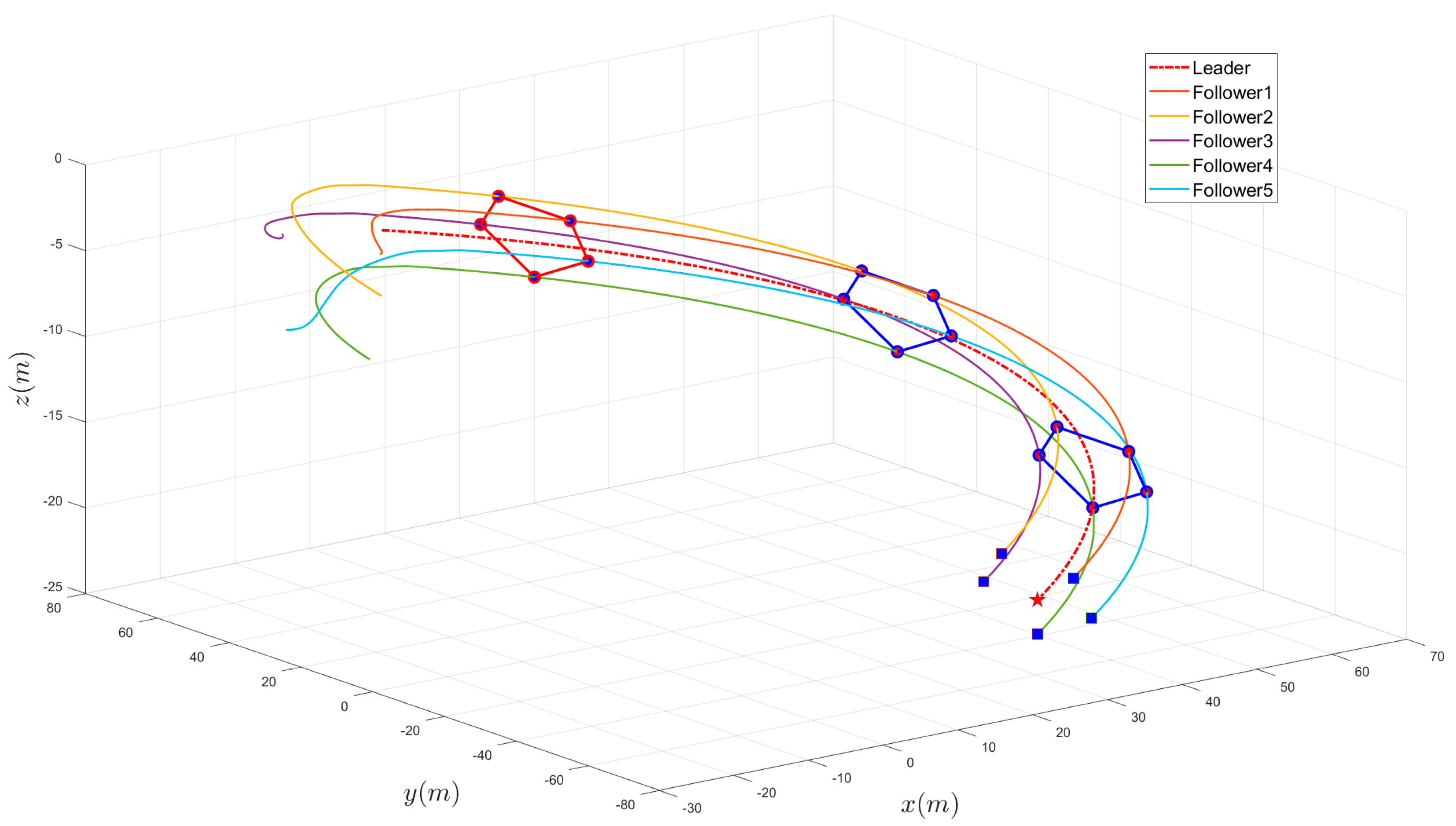
Based on Lemma 1 and the parameters mentioned above, one can easily calculate that the settling time of the formation task is $T=T_{CFGT}+T_{ATT}=12.84s$, which means all the followers can generate the desired trajectories according to the formation vector and track their desired trajectories within the settling time $T$. Figure 5 depicts the three-dimensional time-varying trajectories of six AUVs without obstacles. The five blue circles surrounding by the red pentagon denote the positions of the followers at settling time $T$. The red star represents the final position of the leader AUV and five bule squares represent the final positions of five follower AUVs. As shown in Figure 4, the formation is completed before $T=12.84s$, and the formation can be maintained till the end of the mission. The result shows that, under the hierarchical framework and designed controllers, AUVs can complete the formation task well within a fixed time.

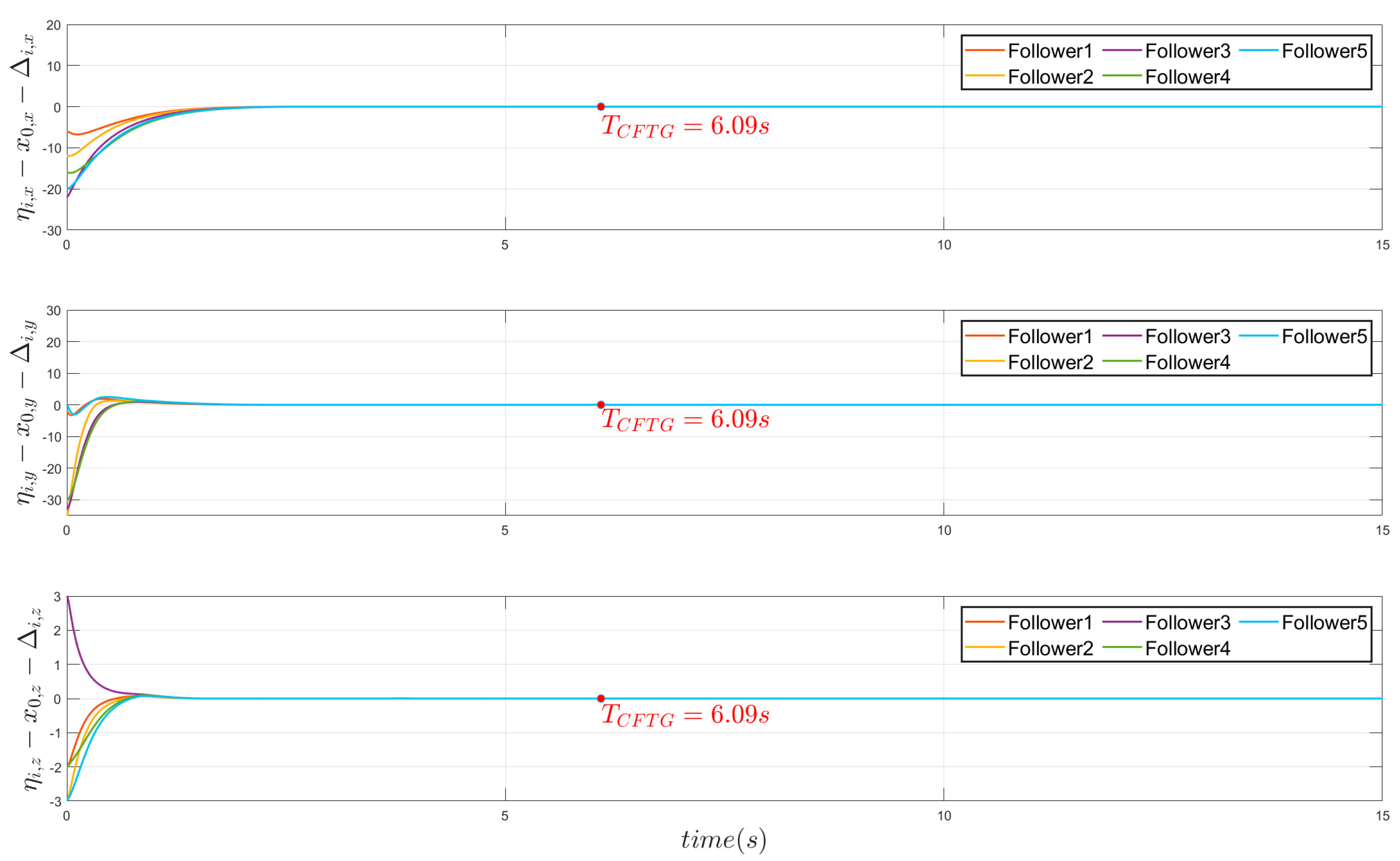
Figure 6 illustrates the deviation between the trajectories generated by the CFGT Layer and the formation task requirements under obstacle-free conditions. This error metric serves as a critical indicator of the layer’s trajectory planning accuracy, where lower values signify a closer alignment with the prescribed formation objectives. The simulation result shows that all the errors along the $x$-, $y$-, and $z$-axes converge to zero within the settling time $T_{CFTG}=6.09s$. The CFGT Layer generates accurate trajectories for AUVs within a fixed time.

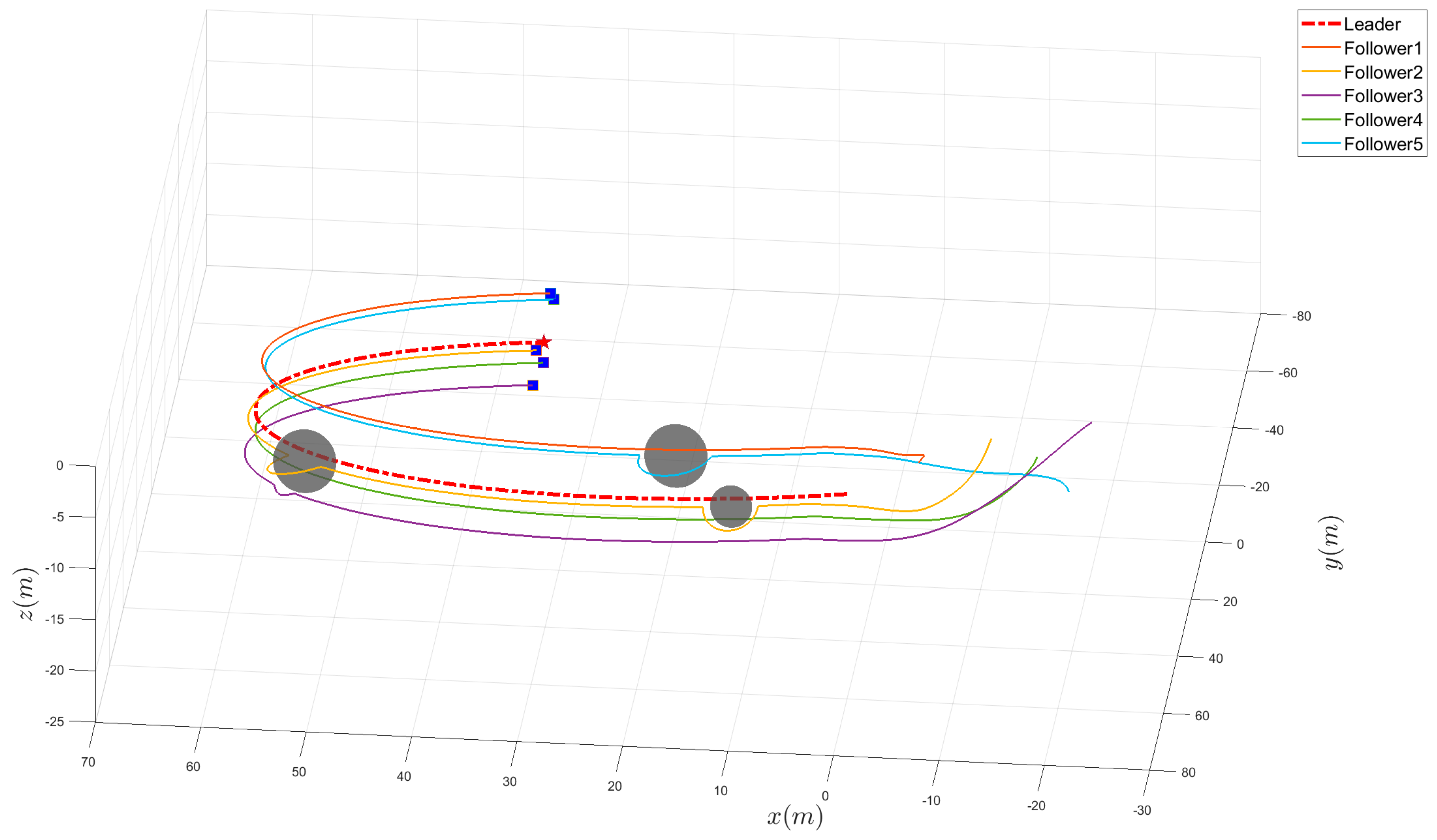
Second, an analysis was conducted for the case involving obstacles in proximity to the AUVs’ trajectories. Define state vector $O_{bi}=[x_{obi},y_{obi},z_{obi},R_{obi}]$ to express the three-dimensional positions and radius of the obstacle. Assume there exit three obstacles, and their state vector were set as $O_b=[10.42,69.08,-4.18,2 ; 52.9,38.29,-10.34,3 ; 17.41,42.41,-7,3]$.

Figure 7 depicts the three-dimensional time-varying trajectories of six AUVs with obstacles. Three obstacles are represented by gray spheres. In Figure 7, follower 2, follower 3, and follower 5 are influenced by the three obstacles. Under the improved artificial potential field methods, it ensures that the AUVs will not collide with obstacles near them and can immediately return to the formation after exiting the danger zone. The result shows that, based on our proposed methods, AUVs can achieve collision-free formation.

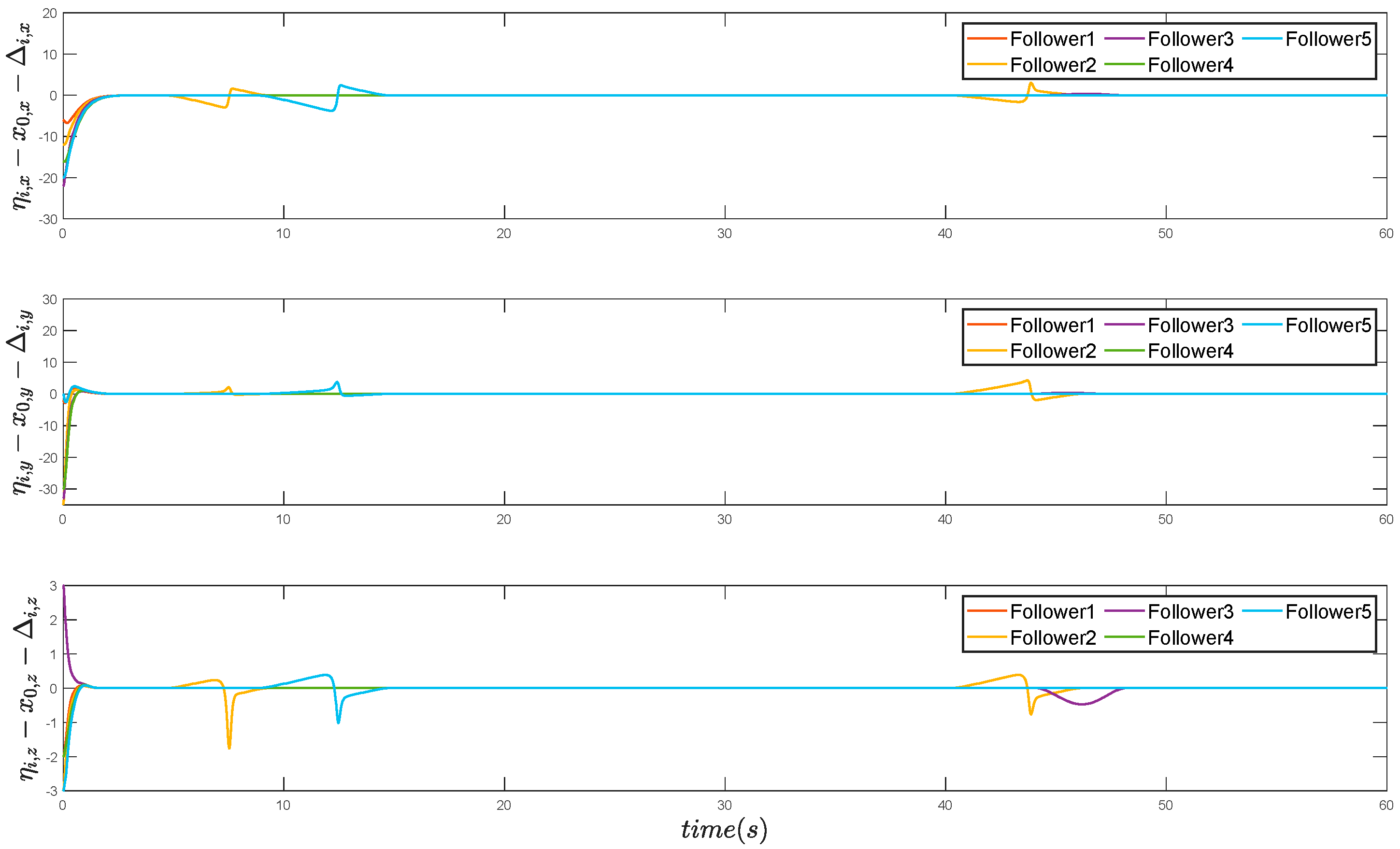
In Figure 8, the obstacle avoidance situation of AUVs is more evident when encountering obstacles. The three fluctuations in Figure 8 represent the follower 2, follower 3, and follower 5 are sailing near obstacles. At this point, under the improved APF algorithm, these AUVs temporarily deviate from the formation to avoid obstacles. After these AUVs move away from the obstacles, the formation error decreases to zero rapidly, indicating that the formation is reconstructed quickly.

6.2. Comparison of Designed Trajectories Tracking Algorithm and Current Results

In this section, the simulation studies focus on a single trajectory that generated in the CFTG Layer to analyze the performance of trajectories tracking controller. The comparison of the designed trajectories tracking algorithm and the current results (AF-DSC [33] and MPC [34]) was conducted to verify the efficiency and superiority of our proposed adaptive fixed-time trajectories tracking controller.

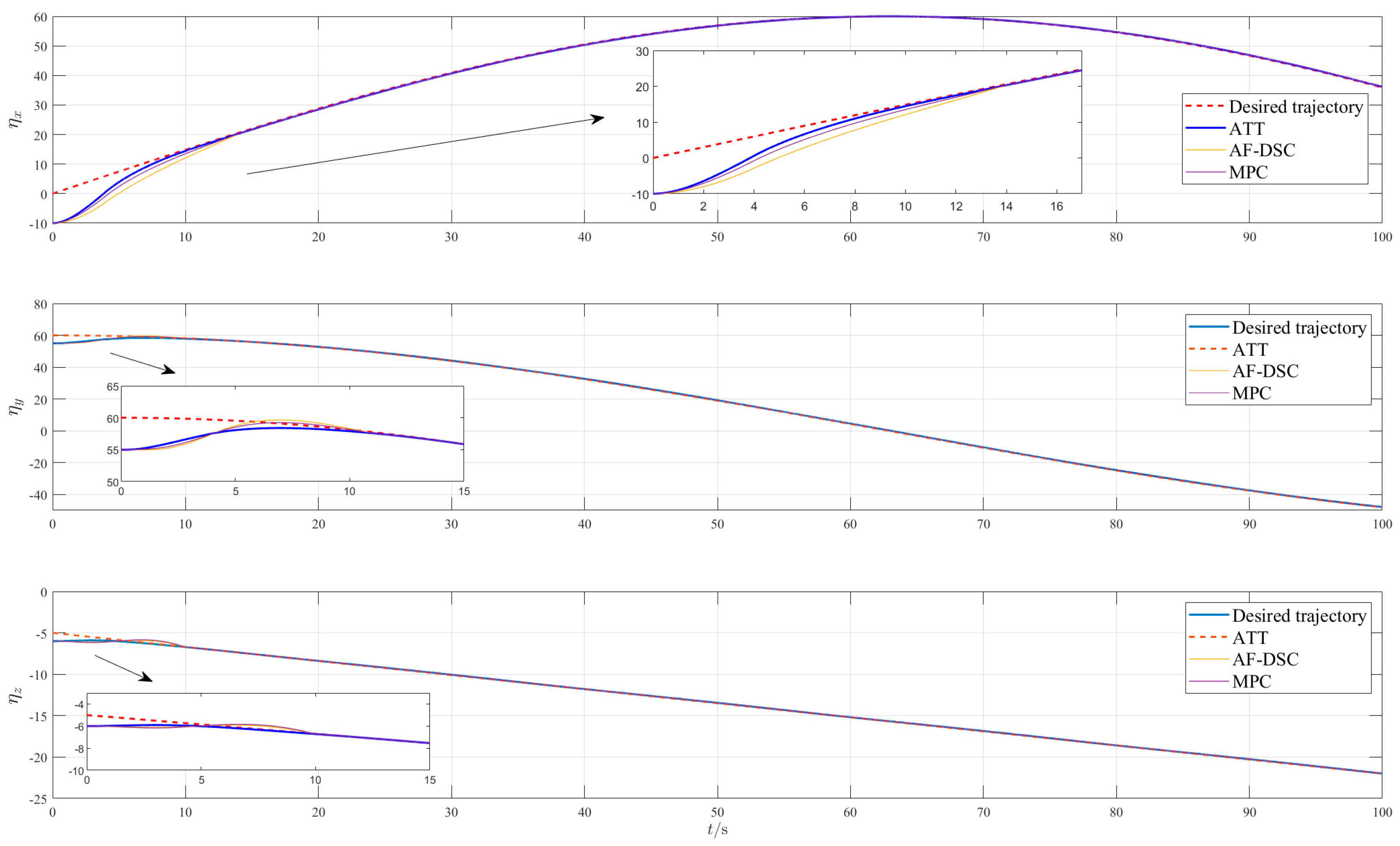
Aiming at a single AUV, Figure 9 presents the three-dimensional trajectory tracking results, while Figure 10 displays the desired and actual trajectories along the three axes. Compared to AF-DSC and MPC, the ATT has a faster response speed and reduced overshoot in trajectory tracking. In addition, the tracking accuracy has also been improved. In practical underwater environments, by utilizing the adaptive fixed-time trajectory tracking methods, system speed and stability can be enhanced, which will contribute to improved trajectories tracking performance.

Figure 11 depicts the control input of the underactuated AUV. As shown in Figure 10, compared with AF-DSC and MPC, the control inputs in the ATT Layer can be limited to within the prescribed ranges because of the designed auxiliary compensation system when suffering from the issue of input saturation. Based on the above analysis, it can be concluded the proposed hierarchical adaptive fixed-time controllers are reliable and can achieve a better formation performance.

7. Conclusions

In this article, we designed a hierarchical adaptive fixed-time formation control method for multiple underactuated AUVs subject to uncertain parameters, external disturbances, and input saturation. This hierarchical framework decouples AUVs’ formation requirements and individual control challenges into two distinct layers: the CFGT Layer and the ATT Layer. Specifically, the CFGT Layer functions as virtual AUVs, and a fixed-time consensus-based controller is developed to generate desired trajectories for the AUVs, meeting the demands of complex formation tasks. Meanwhile, considering the obstacles in the underwater environments, an improved APF methods is proposed to address the issue of the target point being too close to obstacles. In the ATT Layer, an auxiliary compensation system is constructed to overcome the saturated inputs. Furthermore, we design the adaptive fixed-time controllers to handle the uncertain parameters in the model, enabling underactuated AUVs to track the desired trajectory precisely. To increase the convergence speed, both layers can converge within a fixed time under the designed controllers. The numerical simulations conclusively validate that all hierarchical layers successfully attain their designated objectives, with AUVs achieving precise fixed-time formation control. And the comparative analysis with other methods substantiates the better performance of the hierarchical formation control method.