A Discrete-Element-Based Approach to Generate Random Parameters for Soil Fatigue Models

Abstract

The structural reliability of bottom-fixed offshore wind turbines is generally influenced by the dispersion of and variability in soil properties, which affect their ultimate capacity, serviceability, and both the short- and long-term fatigue. During an earthquake, the soil–pile system is subjected to intense cyclic loads that can lead to stiffness and strength degradation, typically captured through cyclic soil models. Calibration of soil parameter variability is fundamental for reliable structural assessments of wind turbine integrity. In this study, a method to generate randomness of the parameters affecting cyclic soil degradation models is proposed. Fatigue parameters are quantified through random cyclic undrained triaxial tests conducted using the Discrete Element Method. Deterministic simulations are first performed based on experimental results from the Liquefaction Experiments and Analysis Project for validation. Subsequently, variability in the initial particle size distribution functions is introduced to generate random soil samples, and triaxial simulations are repeated to quantify the dispersion of soil fatigue parameters. The proposed procedure is then applied through Monte Carlo simulations on the IEA 15-MW reference wind turbine, which is subjected to both short- and long-duration earthquakes. The results demonstrate the significant impact of soil degradation on the bending moment envelope, as well as the effect of soil uncertainty on tower fatigue, assessed using the damage equivalent load approach.

1. Introduction

Offshore wind structures are continuously subjected to cyclic loading induced by wind and waves and, occasionally, earthquakes. Because of their typical features of being tall, flexible, and top-heavy structures as well as due to the inherent lack of structural redundancy, fixed-bottom offshore wind turbines (OWTs) are extremely sensible to vibrations and tilting. Their dynamic response affects the long-term fatigue and serviceability of the whole structure, resulting in a reduction in energy production and, in extreme cases, causing damages, collapses, or premature decommissioning [1].

To avoid unsatisfactory performances, an assessment of the structural safety and of the service and fatigue reliability needs to be performed through high-fidelity models incorporating the various sources of uncertainty that affect their dynamic response.

Mardfekri et al. [2] proposed a probabilistic formulation to assess service reliability by creating a virtual experiment database of 80 configurations of detailed three-dimensional nonlinear finite element models, defining a design space of 22 model parameters. Zorzi et al. [3] applied a probabilistic approach along with a reliability framework to verify the tilting requirement of the monopile foundation, considering random variables of the soil and load input values. Yu et al. [4] used a multi-objective optimization technique to achieve the robust design of monopile foundations, considering the uncertainties in 23 model inputs comprising structural, dynamic loads and soil parameters. Johari et al. [5,6,7] carried out probabilistic reliability analyses to investigate the liquefaction potential, finding that the uncertainty of the soil relative density is one of the most effective parameters in the safety factor of liquefaction.

The above studies have demonstrated the fundamental role of correctly characterizing the parameters governing the soil–pile interaction phenomenon for a reliable assessment of the dynamic performance of OWTs. Moreover, in addition to the characterization of the various sources of uncertainties (see, e.g., [8,9]), the modelling of the variation in the soil uncertain parameters under cyclic loading is an additional related problem to be considered. The study conducted by Schafhirt et al. [10] highlighted the sensitivity of the variation in the soil parameters on long-term fatigue during the lifespan of a wind turbine; findings showed that the damage equivalent bending moment at the mud-line can increase or decrease according to the cyclic softening and hardening behavior of the soil. Moreover, the variation in the soil properties scatters the modal parameters of the wind tower, such as natural frequencies and damping (see, e.g., [11,12,13,14,15]). The variation in the soil properties can be linked to the undrained condition during the cyclic response of the wind turbine foundations, which generates accumulation and dissipation of transient excess pore pressure. Although the circumstances do not always occur as shown in the study by Stuyts et al. [16], medium–low permeability and high-intensity loading can develop pore pressure build-up that produces subsidence around the upper portion of the pile and reduces the overall capacity of the foundation, leading to large cumulative pile deformation (Sun et al. [17]). Similar outcomes are obtained in the paper by Sun et al. [18], when a wind tower was subjected to large deformations induced by seismic ground motions.

Although several non-generally accepted standardized approaches exist for the evaluation of cyclic load-bearing capacity [19], the changes in the soil’s internal state can be explicitly modelled by using effective stress methods [20], i.e., with a fully coupled soil skeleton–pore fluid scheme (see, e.g., [18,19,20]) or, implicitly, by means of relationships formulated as a function of the number of loading cycles, usually defined as soil-fatigue-based problems (see, e.g., [21,22,23,24,25]).

Regardless of the type of approach used for capturing the variation in the soil properties. such as stiffness, strength, and damping, several model parameters have to be determined (see, e.g., [26,27,28,29]) through substantial experimental data from laboratory-based element tests (cyclic triaxial or cyclic simple shear tests) or in situ tests.

As seen earlier, accounting for the uncertainty in the parameters governing this phenomenon is essential for conducting a reliable assessment of wind turbine performance. Without relying on assumptions about the normality of the parameter distributions (as was carried out in [2,3,4,30]), an extensive geotechnical campaign of undrained cyclic experimental testing should be conducted to improve the estimation of the uncertain quantities (see, e.g., [31,32,33]). On the other hand, accounting for every factor affecting the cyclic behavior makes uncertainty quantification costly and unfeasible. Alternatively, non-probabilistic or data-driven approaches (see, e.g., [34,35,36]) can also be adopted.

In order to increase the number of data points used to infer the properties of probabilistic or non-probabilistic distributions, Maksimov and Tombari [37] showed that the Discrete Element Method [38] can be used as an interesting and fast numerical tool for performing numerical cyclic undrained triaxial testing for calibrating cyclic degradation models. This approach can be exploited to consider any factor that affects the cyclic soil behavior such as the fabric, the particle size distribution, the initial void ratio, the confining pressure, and the magnitude of the cycle stress or strain.

The Discrete Element Method (DEM) has already been shown to be effective in simulating shearing and triaxial testing (see, e.g., [37,38,39,40,41,42]), cyclic triaxial testing (e.g., [43,44,45,46,47,48,49,50]), and soil–pile interaction phenomena (see [51,52,53,54]).

In this study, a methodology is proposed to calibrate cyclic soil degradation models through numerical undrained cyclic triaxial testing of soil samples, considering an inherent randomness of the particle size distribution. The calibrated model parameters are then used for performing a Monte Carlo simulation to account for the degradation of cyclic p-y soil–pile interaction for seismic and fatigue analyses; in addition, the proposed methodology can also be used for the calibration of plasticity model parameters, waiving the normality assumption.

The DEM model is calibrated and validated through experimental tests carried out by Vasko [55] and ElGhoraiby et al. [56] for the Liquefaction Experiments and Analysis Project (LEAP). Finally, numerical cyclic triaxial testing is conducted on several realizations of particle size distribution functions with increasing degrees of uncertainty measured by the statistical coefficient of variation (COV) measure [57] to investigate the impact induced by the randomness of the PSD on the soil degradation.

The proposed approach exploits the Discrete Element Method (DEM) to generate distribution functions for soil fatigue parameters by adopting a physical framework that accounts for uncertainty in the particle size distribution (PSD). This completes previous studies on fatigue reliability and liquefaction potential, which relied on assumed probability distributions of input parameters. The method can be used to generate random parameters for Monte Carlo simulations and data-driven approaches, and it demonstrates, for the first time, an alternative means of deriving probability distribution functions for soil parameters.

2. Cyclic Soil Degradation Models

Cyclic loading causes a change in the internal state of the soil, which can be measured as the variation in the void ratio or as the excess pore pressure build-up under drained and undrained conditions, respectively. This variation is mainly responsible for the gradual degradation and hardening of the strength and stiffness that occurs during cyclic loading; in extreme cases of undrained conditions, liquefaction or cyclic mobility can be reached, resulting in a loss of the foundation’s bearing capacity.

A practical approach to simulate the effects of hardening or softening of the lateral soil–pile reaction is through the Beam on Nonlinear Winkler Foundation (BNWF), which extends Winkler’s model [58] to account for various sources of nonlinearities, such as gapping, cyclic behavior, and hardening/degradation [59,60]. The BNWF model has a reduced number of degrees of freedom compared to 3D solid models, allowing for a greatly reduced computational complexity. Therefore, this approach can be conveniently used to assess the structural performance, fatigue, and reliability of offshore wind turbine foundations, where several simulations have to be performed. Whilst the monotonic behaviour of the lateral soil–pile reaction (p-y backbone curve) can be obtained through different analytical and numerical approaches (see, e.g., [61,62,63,64,65,66,67,68,69,70,71]), cyclic degradation and hardening are usually captured through empirical functions used to describe the variation in the strength and stiffness with the number of cycles.

This approach is generally called soil-fatigue-based modelling [26], which defines a degradation or damage index as a function of the equivalent number of cycles of the investigated time-history quantity. The approach was first developed by Idriss et al. [24] for capturing the degradation of clays through the degradation index $\delta$, defined as follows:

$$\delta = N_c^{-t},$$

(1)

The degradation index $\delta$ ratio is defined as the ratio between the secant shear modulus at the current cycle $N_c$ and $N=1$, and $t$ is an empirically calibrated degradation parameter. This approach has been generalized for sands and clays by Allotey and El Naggar [59], who developed a stress-independent nonlinear damage accumulation model based on an elliptical degradation function as follows:

$$\delta =1+\left({\delta }_f-1\right)·{\left[1-{\left(1-D\right)}^{ϴ}\right]}^{{\displaystyle \frac{1}{ϴ}}},$$

(2)

where $D={\displaystyle \frac{N_c}{N_U}}$ is the current cumulative damage with respect to the number of cycles to liquefaction, $N_U$, ${\delta }_f$ is the maximum degradation, and $ϴ$ is a curve shape parameter. The advantage of this model is the capacity to govern the degradation rate through the curve shape parameter and, differently from the model of Equation (1), to simulate concave or convex evolution of the cyclic softening or hardening. Therefore, several types of soils, from soft to hard clays and loose to dense sands, can be considered. More details on the cyclic degradation models and their benefits and drawbacks are discussed in the study by Allotey and El Naggar [26].

The degradation index $\delta$ of Equation (2) is used as the multiplier of the initial stiffness and ultimate capacity of “p-y” curves to account for cyclic hardening or degradation of the stiffness or strength, respectively.

The model of Equation (2) requires knowledge of a failure condition and a stiffness/strength evolution function, which generally have to be empirically obtained through cyclic triaxial testing.

Although cyclic soil degradation models require fewer parameters than advanced constitutive soil models, conducting experimental cyclic testing is expensive and highly demanding; for a reliable analysis, every factor affecting the degradation, such as effective confining pressure, void ratio, particle size distribution (PSD), and strain/stress level, should be analyzed for a comprehensive characterization of the soil behavior. Moreover, in the case of considering soil uncertainty for conducting a reliable geotechnical analysis, a large number of cyclic tests are required to infer distributions of the parameters making the characterization unfeasible to conduct experimentally.

Therefore, following the procedure initiated by Maksimov and Tombari [37], a methodology is developed in this paper, depicted in Figure 1, to generate computational Discrete Element Method [38] models used to extend a few experimental analyses with numerical simulations, providing robust statistics of the distributions of the soil properties. The proposed approach is suggested to be a tool for conducting uncertainty quantification or reliability analyses as well as for multi-scale analysis for the calibration of continuous constitutive models.

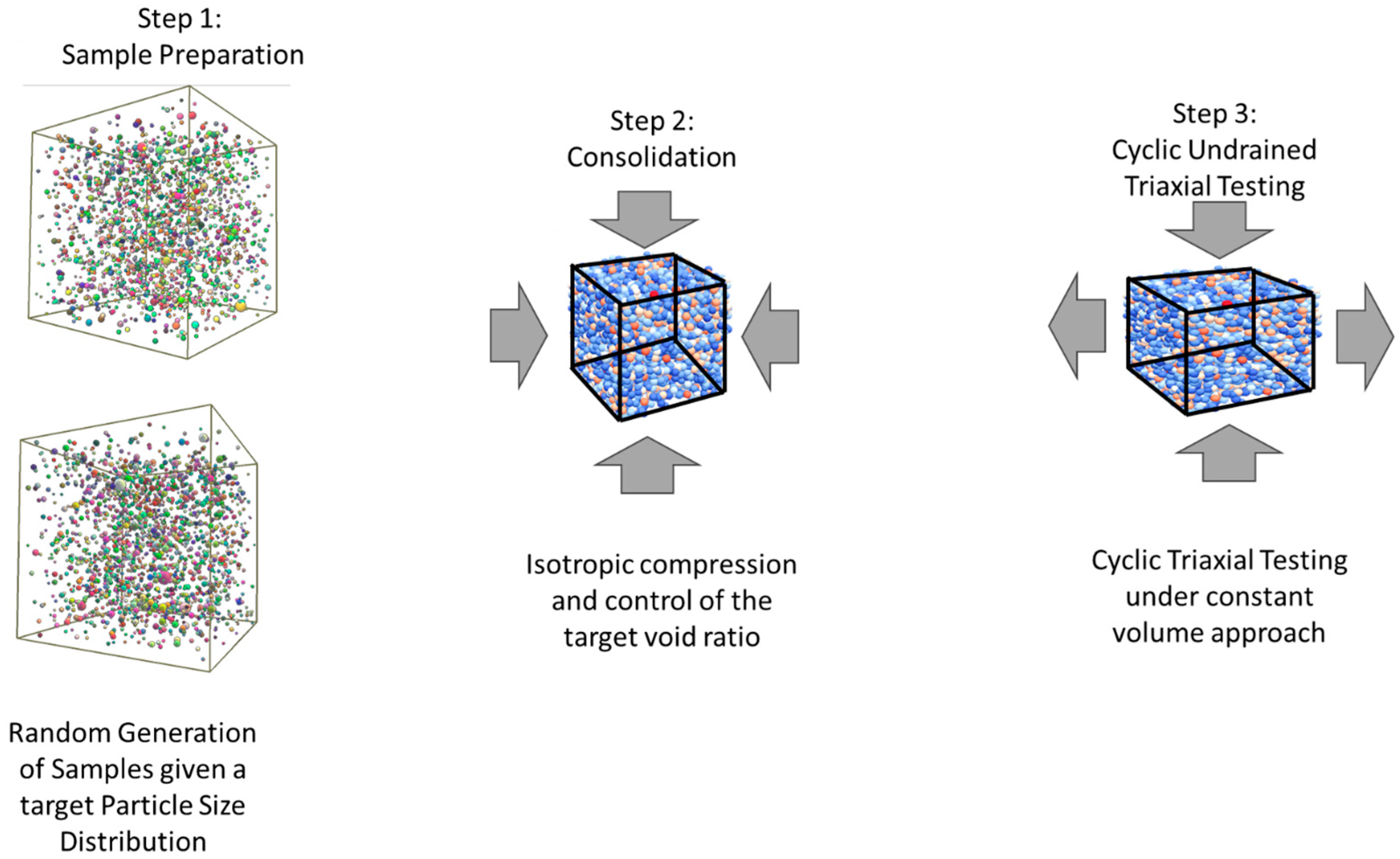
3. Undrained Cyclic Triaxial Discrete Element Testing

The Discrete or Distinct Element Method [38] is based on the analysis of the dynamic equilibrium of an assembly of particles subjected to interaction forces and moments caused by an artificial interpenetration of the particles. At the contact point between two touching particles i and j, two perpendicular forces are generated, as depicted in Figure 2; one is aligned with the line connecting the two particle centers, $N_{i,j}$, and one is perpendicular to it, $S_{i,j}$, representing the normal and tangential forces, respectively. Additionally, a couple could also be added to equivalently consider the rolling resistance, otherwise neglected when perfect spheres are used to model each soil grain (e.g., [72,73,74]).

The set of forces acting at the contact point can be determined using several contact models such as the Cundall–Strack elastic perfectly brittle contact model or the Hertz–Mindlin no-slip contact model [75]. These forces and moments contribute to the dynamic translational and rotational equilibrium of the whole assembly of particles, the equations of which can be solved through an explicit time integration scheme such as the “leap-frog” algorithm [76], obtained by modifying the Verlet difference scheme [77]. The objective of the analysis is to obtain the updated particle position at each time $t$; after detecting the new contacts or collisions, new interaction forces are computed to determine the new state of equilibrium. This method has been largely used to simulate the macroscopical behavior of granular material, proving typical theoretical aspects such as dilatation and critical state behavior (see, e.g, [37,38]) as well as liquefaction onset (see, e.g., [78,79]).

By explicitly modelling the contact interactions of an assembly of discrete particles, the discrete element framework is governed by simpler relationships than those used for continuous models, which generally require several parameters to fully define the undrained soil behavior in terms of stress-dependent elasticity, yielding, and hardening/softening as well as cyclic degradation. Under the DEM framework, the macroscopic behavior of the soil is intrinsically accounted for, considering physically meaningful parameters related to the soil fabric, such as the grain size and shape profile, the spatial distribution of the grains and voids, whilst just the micro-mechanical behavior is described by constitutive relations based on elasto-plastic friction models.

In this paper, the open-source code YADE [39] is used for the modelling and simulation of the cyclic triaxial testing; nevertheless, the proposed procedure is general and can be adopted with any similar codes.

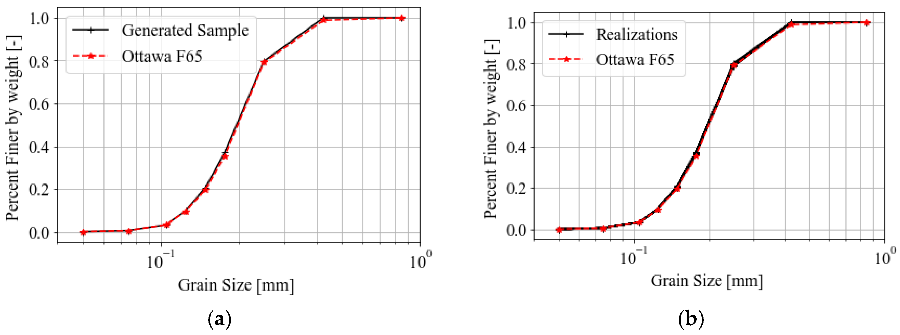
3.1. Random Sample Generation

The first step entails the generation of numerical specimens to express the uncertainty of one or more physical properties. In this paper, the randomness of the soil structure is assigned to the size, distribution, and arrangement of the grains; this causes a modification in the inherent anisotropy of the soil properties as well as in the re-arrangement of the soil fabric during loading. The randomness or uncertainty can also be applied to different properties than the ones used in this paper, such as the void ratio, relative density, fines content, or grain shape. These evaluations are case-specific and do not alter the proposed methodology to calibrate cyclic degradation models following the next steps in Section 3.2 and Section 3.3. To express the uncertainty of the soil structure, the soil grains are randomly generated according to a given particle size distribution (PSD) function, determining the distribution of the particles’ radii as a function of the cumulative fractions of the particles’ masses. This can be seen as a statistical cumulative distribution function used to randomly generate the assembly of particles; each particle is then spatially allocated in an empty space, i.e., a void, within a cubic cell of given dimensions to avoid any initial overlap between any two grains. Therefore, the resulting packing is in a gas-like state under stress-free conditions. Although different shapes could be used [44], spherical particles are generated in this investigation, where the effect of the actual grain shape is herein approximately accounted for through the addition of a rolling stiffness. Each cell is defined as the representative volume element (RVE) of the investigated soil, and its dimensions are also reduced by using periodic boundary conditions.

Because of the random generation, this first step is affected by a certain level of randomness or deviation from the target PSD; the error reduces with the increase in the cell size or, equivalently, the number of generated particles. Several soil samples are generated by modifying the target particle size distribution function in similarity with what was proposed by Phoon and Kulhawy [8], hence considering each generated PSD function as the sum of a mean-valued function, $P_{d,i}^{target}$, with a normally distributed fluctuation as follows:

$$P_{d,i}=P_{d,i}^{target}\left(1+w_i·COV\right),$$

(3)

where $P_{d,i}$ is the percentage finer at the sieve diameter, $d,i$, $P_{d,i}^{target}$ is the percentage finer of the target distribution, $w_i$ is a random number drawn from the standard normal distribution, and $COV$ is a given coefficient of variation. When the available amount of information is high, Equation (3) can be modified by replacing the average $COV$ with ${COV}_i$ to apply a different dispersion for each percentage passing. In this study, an average $COV$ is used to cover different scenarios from laboratory-controlled samples to average statistical metrics from databases.

It is worth mentioning that the average randomness, ${COV}_t$, measured from the generated samples, is affected by the initial dispersion of the particles’ radii and by the assigned fluctuation in the percentage finer measured through the coefficient of variation $COV$. Examples of generated samples using Equation (3) are depicted in Figure 3a for $COV=0$, used for the deterministic analysis, and in Figure 3b for $COV=0.005$ for assessing the repeatability of the numerical experiments.

3.2. Numerical Consolidation Phase

In the second stage, the cloud of particles is subjected to isotropic compression, ${\sigma }_0$, by moving the fictitious cell boundaries uniformly until the mean stress reaches a desired confining pressure. The shrinking of the cell volume allows the particles to get closer and closer until they start to overlap, generating compressive and tangential forces. The forces are linked to the contact model adopted for simulating the microscale behavior described in Section 4.1.

At this point, by keeping a constant confining pressure, the interparticle friction angle governing the tangential forces is reduced iteratively, causing a decrease in the void ratio until the target value is achieved. This procedure has been adopted to determine a soil sample with a given PSD and void ratio under a fixed confining pressure. It is worth mentioning that at this stage, the parameters of the contact law are artificial, and their values will be replaced before the start of the cyclic testing at Step (3), with the calibrated ones, without changing the conditions reached during Step (2).

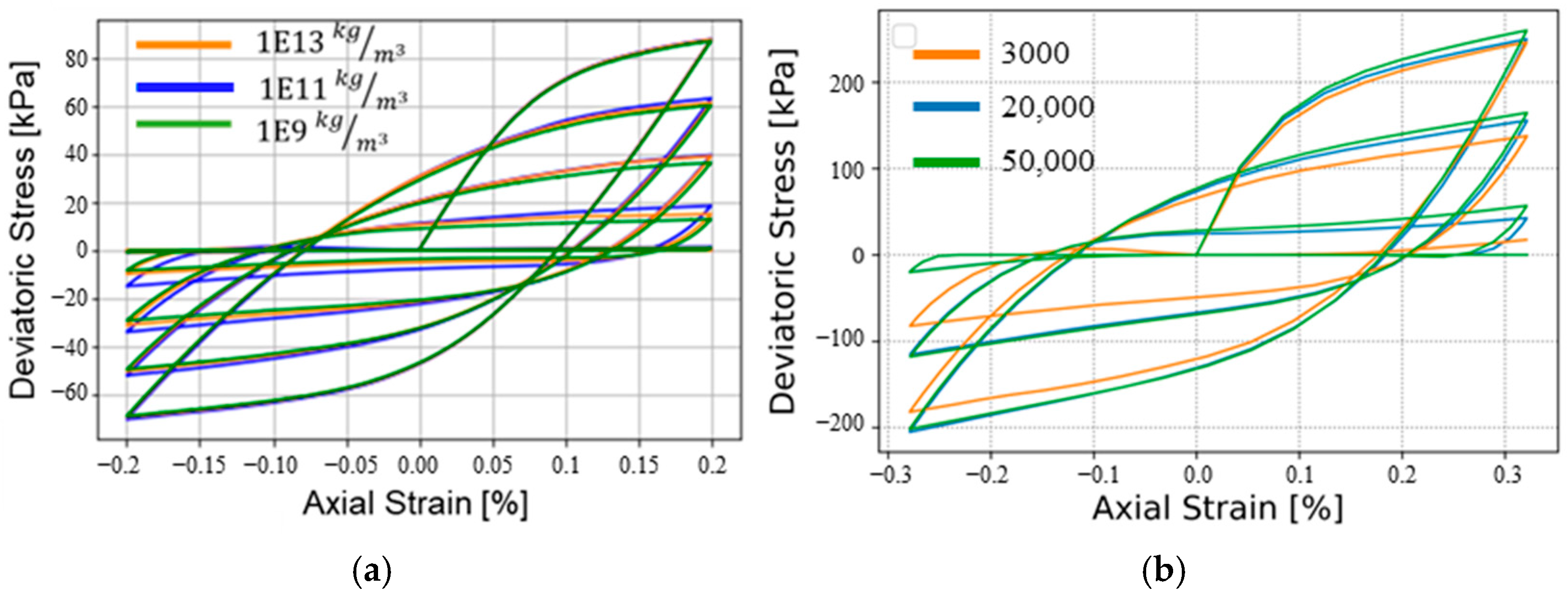
3.3. Strain-Controlled Cyclic Triaxial Testing

Once the sample is prepared, the third stage consists of strain-controlled cyclic triaxial testing. The calibrated parameters of the constitutive models are set, and after an initial re-stabilization of the confining pressure without modifying the void ratio, the assembly of particles is subjected to a cyclic deviatoric stress state. This is performed by controlling the strain amplitudes of the sample boundaries; because the pore fluid pressure is not directly modelled, the undrained conditions are imposed by constraining the strains in the three directions [37,49], as follows:

$${\epsilon }_{xx} = {\epsilon }_{yy}{ = -0.5·\epsilon }_{zz},$$

(4)

in which ${\epsilon }_{xx}$ and ${\epsilon }_{yy }$ are the strains of the lateral boundaries of the periodic cell, whilst ${\epsilon }_{zz}$ is the axial strain aligned with the cyclic direction during the triaxial testing. Equation (4) defines the relations required to maintain a constant volume during the deviatoric deformation. The cyclic behavior is then imposed through the following relation:

$$\dot{\epsilon } = CSA·2\pi f·\mathrm{c}\mathrm{o}\mathrm{s}\left(2\pi ft\right),$$

(5)

where $f$ is the frequency (fixed at 0.0083 Hz as in Kutter et al. [80]), $CSA$ is the cyclic strain amplitude, and $t$ is the current time in seconds. The cyclic testing terminates when the soil sample reaches the failure condition, defined as a reduction in the mean stress to 5% of the initial value. This condition is considered similar in increasing the excess pore pressure to 95% [56].

4. Ottawa F65 Sand Discrete Model Characterization

Whilst the method proposed in Section 3 can be applied to a generic cohesionless soil, this paper focuses on the undrained triaxial behavior of Ottawa F65 sand, which has been comprehensively investigated through experimental testing for the Liquefaction Experiments and Analysis Project (LEAP) [80]. Ottawa F65 sand is an inert, white silica sand of rounded grains with a quartz content of 99.7%; it is classified as a poorly graded sand with a fine content of less than 0.5%. The median values of the maximum and minimum void ratios, i.e., e_max = 0.78 and e_min = 0.51, are considered in the present paper. Further specific details can be found in the report produced for the LEAP [80]. In this section, the results from the experimental triaxial testing of Ottawa F65 sand are used for setting up the discrete element model, which will be used for calibrating the cyclic soil degradation models. Validation is also carried out.

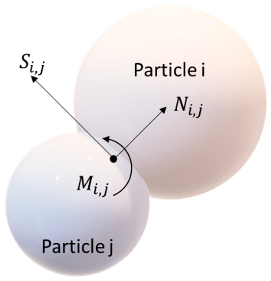
4.1. Contact Law Formulation

The Cundall–Strack elastic perfectly brittle contact law [38] is used to express the force–displacement relation between two touching particles. For each interaction between two particles of radii $r_i$ and $r_j$, defined by the artificial overlap between the i-th with the j-th particle,$d_{ij}$, about the normal direction as well as by the relative tangential displacement, ${\mathsf{\Delta }U}_{ij}$, the induced forces and moments exchanged at the contact point, $c$, are described by the following relations:

$$N_{i,j}=k_n{d}_{ij},$$

(6)

$$S_{i,j}=-{\upsilon k}_n{\mathsf{\Delta }U}_{ij},$$

(7)

$$\mathsf{\Delta }{M}_{i,j}=-{\alpha }_r·{\upsilon k}_n·r_i·r_j·\mathsf{\Delta }{\theta }_{ij},$$

(8)

in which $\upsilon$ is the ratio between shear and normal stiffness, $k_n$, and ${\alpha }_r$ is the rolling stiffness coefficient governing the incremental moment caused by the relative rotation, $\mathsf{\Delta }{\theta }_{ij}$, between the two particles. The normal stiffness, $k_n$, is the harmonic mean of the two springs in series at the contact point, each one of stiffness $k_i=k{\sigma }_0{\left({2r}_i\right)}^2$, where $k$ is a dimensionless stiffness value used to maintain the same level of overlapping at different confining pressures, allowing for a consistent outcome under different conditions.

The nonlinear behavior is defined according to the Mohr–Coulomb rupture criterion for cohesionless soil as follows:

$$‖S_{i,j}‖\le ‖N_{i,j}‖\tan \mu ,$$

(9)

$$‖M_{i,j}‖\le ‖N_{i,j}‖{\eta }_r\min \left(r_i,r_j\right),$$

(10)

where the model parameters are the interparticle angle of friction, $\mu$, and the limiting rolling coefficient, ${\eta }_r$. The operator$‖•‖$ denotes the norm of the force or moment vector.

Therefore, the Cundall–Strack contact law can be fully determined by five parameters, namely, the normal stiffness, $k_n$, the shear-to-normal ratio, $\upsilon$, the interparticle angle of friction,$\mu$, the rolling stiffness coefficient, ${\alpha }_r$, and the limiting rolling coefficient, ${\eta }_r$. The radius, $r_i$, of each i-th particle is obtained according to the procedure reported in Section 3.1 to follow the PSD function of Ottawa F65 sand.

It is worth mentioning that the shear-to-normal ratio, $\upsilon$, is proportional to the macroscopic Poisson ratio; therefore, a value of $\upsilon =0.2$ is used. Therefore, the remaining four parameters are calibrated to capture from the experimental cyclic triaxial testing experimental observed in the LEAP [80] at three different strain amplitudes, i.e., 0.05%, 0.1%, and 0.2%.

In this study, the triaxial testing is executed under quasi-static conditions; hence, the particle mass density does not affect the macroscopic stress–strain behavior, and a high artificial value (hereinafter fixed to $\rho ={10}^{13}{\displaystyle \raisebox{1ex}{$kg$}\!\left/ \!\raisebox{-1ex}{$m^3$}\right.}$) is used to reduce the computational cost of the explicit analyses [40]. Since the minimum critical time step size is proportional to the square root of the density $\rho$ [81]:

$$∆t_{min}=r_i·\sqrt{{\displaystyle \frac{2r_i\rho }{k_n}}},$$

(11)

the time step size can be artificially increased by increasing the particle density; on the other hand, the value is limited by the maximum inertial number in quasi-static conditions, defined as follows:

$$I=\dot{\epsilon }·2r_i\sqrt{{\displaystyle \frac{\raisebox{1ex}{$4$}\!\left/ \!\raisebox{-1ex}{$3$}\right.r_i^3\rho }{V_s{\sigma }_0}}}\ll 0.001,$$

(12)

in which $\dot{\epsilon }$ is the strain rate of the boundary conditions used to simulate the cyclic triaxial testing, and $V_s$ is the volume of the sphere. Figure 4a shows the results obtained on a randomly generated sample of Ottawa F65 sand, where three different particle mass densities were set; the results of the cyclic undrained behaviors show the negligible influence of the particle density when keeping the inertial number lower than 0.001.

Another parameter that affects the simulation is the dimension of the cell determining the RVE; the larger the cell is, the higher the number of generated particles will be. A sensitivity analysis was performed, as shown in Figure 4b, in order to select the right dimension of the cell that provides a good accuracy at the least computational cost; a cell of size 0.004 m containing about 3000 particles was used.

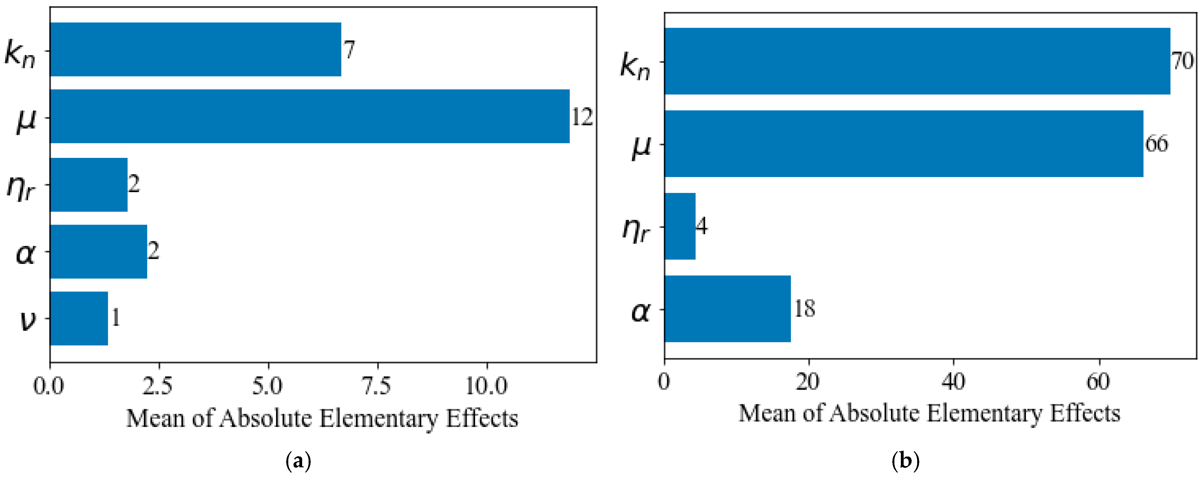
4.2. Morris Sensitivity

Several past studies have investigated the impact of each contact law parameter, focusing on the critical state and volumetric behavior under monotonic triaxial testing [72,82]; these studies were conducted through parametric analyses by changing the parameters once at a time. To assess the sensitivity of the parameters under cyclic behavior, in this study, a global sensitivity analysis using the Morris or elementary effects method [83] is conducted. This method belongs to the global “Once-At-Time” class and is an effective way of screening the importance of each model parameter. The method consists of generating $t_r$ trajectories where the $p$ parameters are changed randomly, once at a time by a pre-defined value obtained by discretizing the overall range in $l$ levels. An elementary effect represents the variation in the outcome of the analyses after each step, normalized by the step size. The ensemble of the elementary effects for each parameter $p$ is analyzed statistically as the mean of the absolute value. The mean value determines the overall influence of each factor on the output, ranking from the most to the least important. The complete procedure is explained in the study by Saltelli et al. [84].

In this paper, $t_r=50$ trajectories were generated for $p=5$ parameters with $l=6$ levels of discretization. The ranges of variation in the parameters that were tested were $k=\left[{1\times 10}^7-{5\times 10}^7\right]$, $\mu =\left[{10}^{°}-{35}^{°}\right], { \eta }^r=[0-0.4]$, $\alpha =[0-3]$, and $\upsilon =\left[0.15-3\right],$ selected in accordance with past experience in DEM analyses (see, e.g., Maksimov and Tombari [37]). The ranking of the factors is illustrated in Figure 5a, demonstrating the importance of the interparticle angle of friction and the contact stiffness on the number of cycles to liquefaction ($N_u)$. As already observed in [72], the interparticle friction value strongly affects the peak deviatoric stress and dilatancy. Since the shear-to-normal ratio, $\upsilon$, turned out to be the least important parameter and generally can be calibrated to match the soil Poisson ratio, the sensitivity analysis was also performed with the four remaining parameters by fixing $\upsilon =0.2$, as previously mentioned. The global sensitivity analysis was conducted for three strain amplitudes, $\mathrm{C}\mathrm{S}\mathrm{A} = 0.1\mathrm{\%}, 0.2\mathrm{\%}$, and $0.4\%$, showing a similar outcome for all the cases.

4.3. Calibration of the Contact Law Parameters

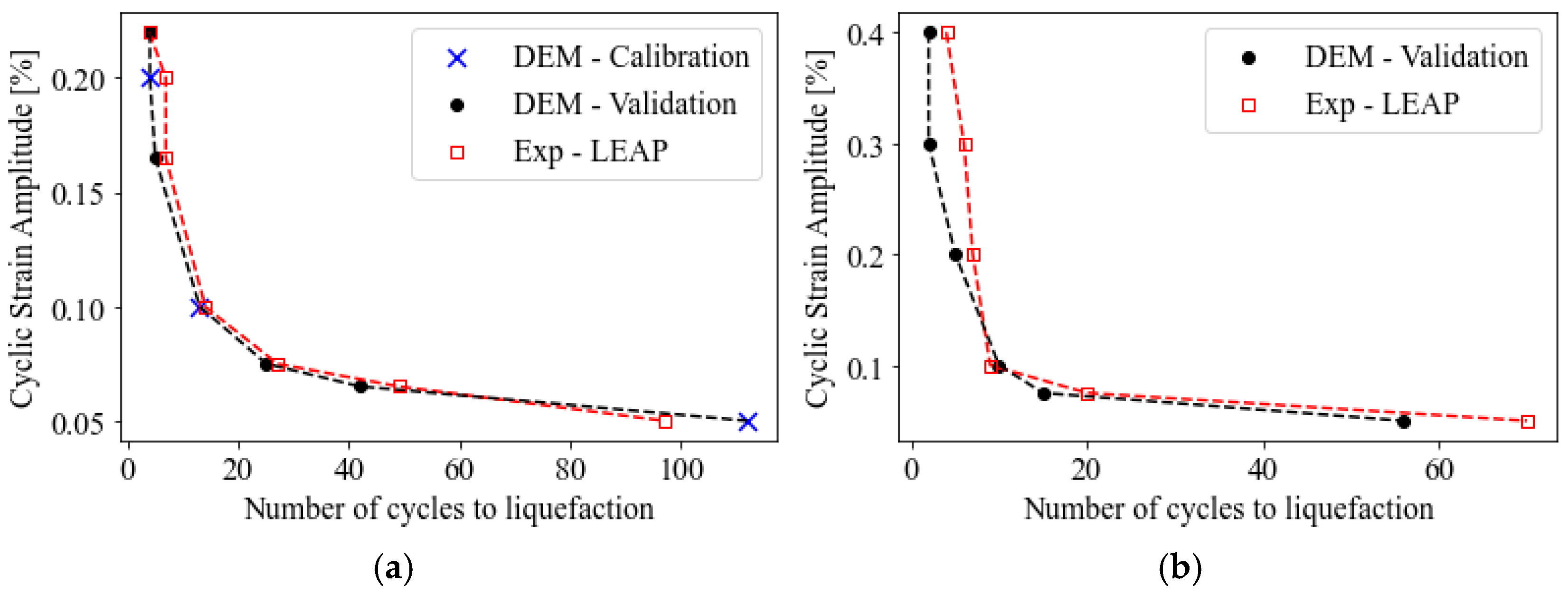
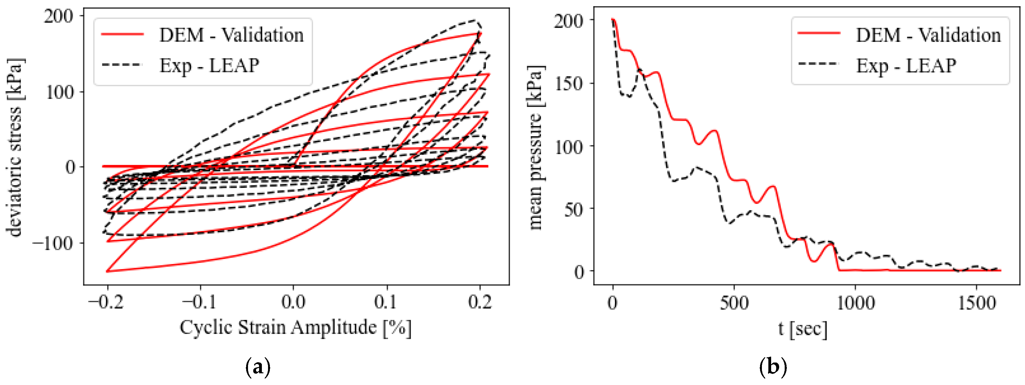
In this study, the experimental $e_z-N_u$ curve (axial strain–number of cycles to liquefaction) from the tests conducted for the LEAP [56] is used as the reference curve for the calibration of the Cundall–Strack law model.

The experimental curve is derived from the results of the strain-controlled cyclic triaxial testing conducted on Ottawa F65 sand with a void ratio of 0.608 and at a confining pressure of 100 kPa.

The number of cycles to liquefaction, generating an excess pore pressure of 95% more than the initial mean effective stress [56], are used as the target values for the calibration approach; they correspond to 4.87, 14, and 97 cycles, conducted at axial strain amplitudes of 0.2%, 0.1%, and 0.05%, respectively.

The remaining results obtained from the different stress levels [56] are used for validating the obtained DEM model, as reported in the next section.

As observed in the previous section, four parameters of the Cundall–Strack law model, i.e., $k_n$, $\mu$, ${\alpha }_r$, ${\eta }_r$, need to be identified. A universally recognized approach of calibration for DEM models does not exist, but an empirical approach [37] or numerical optimization could be performed. It is worth mentioning that the excess pore pressure cannot be directly computed in the investigated model, as explained in Section 3; therefore, the number of cycles to liquefaction is computed here as the number of cycles able to decrease the maximum deviatoric stress to 5% of the initial maximum deviatoric stress.

In this study, a two-step empirical approach is used: first, the calibration of the parameters, $k_n$ and $\mu$, aiming to obtain the experimental maximum deviatoric stress and initial stiffness of the backbone curve, and second, the remaining parameters, $\alpha$ and ${\eta }_r$, are tuned to obtain the target number of cycles to liquefaction. The two steps are then repeated iteratively to obtain a good approximation of the reference curve. A few trial-and-error tests were conducted, and the parameters that provide an acceptable matching are reported in

Table 1. Cundall–Strack law: model parameters.

Parameter	Description	Value
$k$	Dimensionless stiffness value	$2.0 \times {10}^7$
$\alpha$	Rolling stiffness coefficient	$3$
$\mu$	Frictional angle	${15}^{°}$
${\eta }_r$	Limiting rolling coefficient	$0.1$

; they govern the elasto-plastic sliding and rotational behavior between two grains, and they can be seen as an equivalent measure of the soil surface roughness. Therefore, the parameters of Table 1, representing microscopic information, do not change when different distributions of Ottawa F65 sand are generated.

Figure 6a shows, with cross markers, the results of the discrete element triaxial simulation at three different strain amplitudes, in comparison with the experimental curve indicated in red color and box markers.

4.4. Validation

The calibrated DEM model was also validated against further experimental strain amplitudes reported in ElGhoraiby et al. [56], different to those used for calibration; in Figure 6a, the black dots represent the results of the simulation; a good match is achieved against the experimental curve.

Moreover, to validate the model under different conditions, cyclic simulations were been performed at a different confining pressure; the experimental curve was derived from the results of the strain-controlled cyclic triaxial testing performed by Vasko [55] on Ottawa F65 sand with a void ratio of 0.604 and at a confining pressure of 200 kPa.

The results are reported in Figure 6b, demonstrating a good agreement between experimental testing and numerical simulation. Moreover, raw experimental data were also elaborated to verify that the numerical behavior was reliable in terms of cyclic evolution of the stresses and strains; Figure 7a shows the computed cyclic stress–strain behavior for a randomly generated sample, and the evolution of the effective mean stress is plotted in Figure 7b, demonstrating the capability of the constant-volume approach to simulate the undrained conditions without the need of modelling the fluid directly. In both figures, a dashed black curve indicating the experimental results is plotted for a visual comparison with the numerical simulation.

5. Cyclic Degradation Response

Cyclic soil degradation models, briefly reported in Section 2, are usually empirically calibrated through stress- or strain-controlled triaxial or simple shear experiments. As formulated in [26], a comprehensive soil fatigue formulation requires the determination of a failure condition and a fatigue/strength evolution function. The failure condition, representing the full damage, is defined by the ${\sigma }_a-N_U$ and the ${\epsilon }_a-N_U$ curves for stress-controlled and strain-controlled triaxial testing, respectively. Although cyclic stress and cyclic strain methods can lead to different outcomes, a link between the two approaches can be determined through the definition of the cyclic stress ratio, $CSR={\displaystyle \raisebox{1ex}{${\sigma }_d$}\!\left/ \!\raisebox{-1ex}{${\sigma }_0$}\right.}$, defined as the ratio between the maximum deviatoric recorded at the first cycle and the effective confining pressure [85,86]. This function, defined as the $CSR-N_U$ curve, can be used as a representation of the failure condition on soil fatigue models. It is worth emphasizing that the most conventional ${\epsilon }_{zz}^{max}-N_U$ or ${\sigma }_a-N_U$ curves can be used if other soil fatigue models are considered [26]. Some formulations, such as Allotey and El Naggar’s model [59], additionally require the fatigue evolution function, expressed as the degradation index $\delta$ at different cycles.

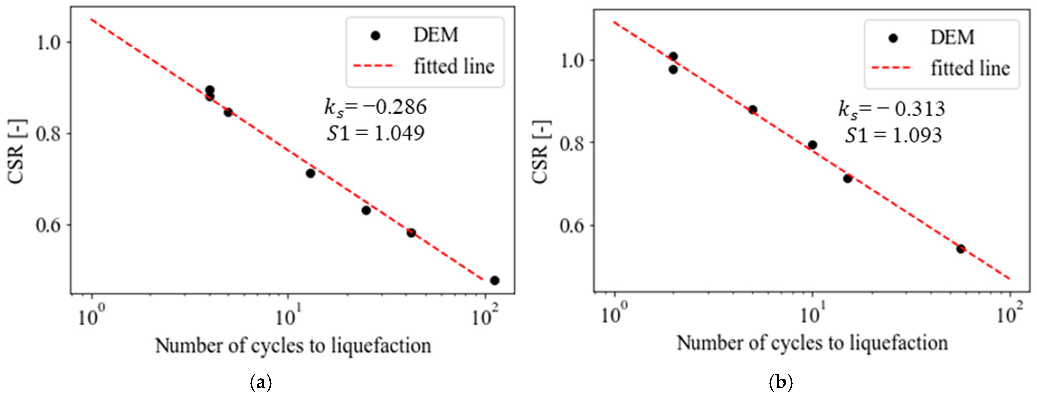
5.1. Deterministic Response

The two functions needed to fully define a fatigue model are derived from the cyclic triaxial tests previously simulated on Ottawa F65 sand.

Figure 8a,b show the $CSR$ curves obtained at different strain amplitudes under an isotropic pressure of 100 kPa and 200 kPa, respectively. The red dashed curve is the linear regression curve fitting the results of each DEM simulation, indicated by black dots. The two parameters required by the soil fatigue models are the slope of the curve, $k_s$, as well as the deviatoric stress ratio at the first cycle, $S_1$.

These two parameters fully define the failure condition in the semilogarithmic space. The results show small differences between the values of the slope of the curve $k_s=-0.286$ at 100 kPa and $k_s=-0.313$ at 200 kPa, as well as the initial stress ratio values, $S_1=1.049$ and $S_1=1.093$. Figure 9 shows the fatigue evolution functions for several cyclic strain amplitudes at a confining pressure of 100 kPa; each marker represents the maximum deviatoric stress computed at the i-th cycle. The minimum degradation index, corresponding to the onset of liquefaction, is determined to be 0.05. Fatigue evolution functions obtained from cyclic testing conducted at a confining pressure of 200 kPa are depicted in Figure 10.

It can be noted that the curvature of the evolution curve varies with the cyclic strain amplitude, changing from a concave to a convex shape with the increase in the CSA. At low cyclic strain amplitudes, the samples manifest a hardening phase characterized by an increment in the initial strength after the first cycle, followed by degradation. This behavior cannot be simulated through Equation (2), and an approximate regression curve is obtained. In this paper, the Allotey and El Naggar hyperbolic model [59] is used to best fit the numerical results through a nonlinear regression procedure to obtain the $ϴ$ parameter of Equation (2); the results are shown in

Table 2. Best-fit shape parameter, $ϴ$, of Equation (2) for several axial strain levels.

$\mathit{C}\mathit{S}\mathit{A}$[%]	0.4	0.3	0.22	0.2	0.165	0.1	0.075	0.065	0.05
${\sigma }_0 = 100 \mathrm{k}\mathrm{P}\mathrm{a}$	1.55	1.22	---	0.92	---	1.03	0.89	---	0.77
${\sigma }_0 = 200 \mathrm{k}\mathrm{P}\mathrm{a}$	---	---	1.21	1.08	1.04	0.92	0.75	0.66	0.53

. It can be observed that the model can cover concave ($\theta <1)$ to convex ($\theta >1)$ shapes. Except for extreme cyclic strain amplitudes, the range of $\theta$ is consistent with the values derived from the experimental results on saturated sands performed by De Alba et al. [87] (i.e., $\theta =0.7-1.1)$.

5.2. Random Cyclic Undrained Response

To assess the impact of the uncertainty on the particle size distribution, soil samples were generated according to Equation (3), where different values of $COV = 0, 0.01, 0.05, 0.1$, were assigned. The set of COV values was parametrically selected to cover different scenarios from laboratory-controlled sands where uncertainty is low due to large variations usually obtained from statistical analysis of datasets. Because of the initial randomness, the computed mean total covariances, ${COV}_t,$ computed on the generated samples are reported in

Table 3. Statistics of the particle size distribution functions of the generated samples.

$COV$	0	0.01	0.05	0.1
${COV}_t$	0.031	0.038	0.069	0.127
Cu	1.69–1.75	1.71–1.77	1.65–1.83	1.61–1.97
Fines content [%]	7.7–10.5	8.3–11.1	7.5–10.5	7.86–12.5
$N^{mean}$ particles	3426	3460	3292	2848

. The number of soil samples was determined to obtain the convergence of the result of the cyclic triaxial testing in terms of the number of cycles; for low COV, a total number of 30 simulations was sufficient, whilst for $COV = 0.1$, 50 samples were required; the distributions of the generated PSD functions for the two different COVs are depicted in Figure 11. Because of the approach used for generating the PSD function, as defined by Equation (3), the dispersion of the higher percentage finer was larger than the lower values. This resulted in a few PSD curves containing larger particles; on the other hand, it is worth emphasizing that the mean function remained the same regardless of the dispersion used in the parametric analysis.

From each of the generated soil samples, consolidation at a confining pressure of 200 kPa, as described in Section 3.2, was conducted to reach an initial void ratio of 0.608 for every specimen. Subsequently, the undrained cyclic triaxial testing of Section 3.3 was carried out by applying three strain amplitudes, i.e., $CSA = 0.1\mathrm{\%}, 0.2\mathrm{\%}, 0.4\mathrm{\%}$. The results in terms of the number of cycles to liquefaction, corresponding to a final degradation index, ${\delta }_f$, of 0.05, are reported in Figure 12 for selected cases of strain amplitudes. Statistics are reported in

Table 4. Statistics of the number of cycles to liquefaction, $N_U$.

	$\mathit{C}\mathit{S}\mathit{A} = 0.1\mathbf{\%}$				$\mathit{C}\mathit{S}\mathit{A} = 0.2\mathbf{\%}$				$\mathit{C}\mathit{S}\mathit{A} = 0.4\mathbf{\%}$
	${\mathit{N}}_{\mathit{U}}^{\mathit{E}\mathit{X}\mathit{P}}$	${\mathit{N}}_{\mathit{U}}^{\mathit{m}\mathit{e}\mathit{a}\mathit{n}}$	${\mathit{N}}_{\mathit{U}}^{\mathit{C}\mathit{O}\mathit{V}}$	$\mathit{R}\mathit{a}\mathit{n}\mathit{g}\mathit{e}$	${\mathit{N}}_{\mathit{U}}^{\mathit{E}\mathit{X}\mathit{P}}$	${\mathit{N}}_{\mathit{U}}^{\mathit{m}\mathit{e}\mathit{a}\mathit{n}}$	${\mathit{N}}_{\mathit{U}}^{\mathit{C}\mathit{O}\mathit{V}}$	$\mathit{R}\mathit{a}\mathit{n}\mathit{g}\mathit{e}$	${\mathit{N}}_{\mathit{U}}^{\mathit{E}\mathit{X}\mathit{P}}$	${\mathit{N}}_{\mathit{U}}^{\mathit{m}\mathit{e}\mathit{a}\mathit{n}}$	${\mathit{N}}_{\mathit{U}}^{\mathit{C}\mathit{O}\mathit{V}}$	$\mathit{R}\mathit{a}\mathit{n}\mathit{g}\mathit{e}$
${\mathit{C}\mathit{O}\mathit{V}}_{\mathit{t}}$			[%]				[%]				[%]
0.005	9	9.03	10.8	7–11	/	/	/	/	/	/	/	/
0.031	9	8.57	27.2	5–16	7	7.1	31.8	5–13	4	2.43	40.7	1–5
0.038	9	7.83	18.6	5–11	7	7.13	27.5	4–11	4	2.2	37.8	1–4
0.069	9	8.23	27.5	4–12	7	7.83	29.9	4–16	4	1.77	59.7	1–6
0.127	9	8.88	56.5	2–31	7	7.36	35.5	3–15	4	1.8	57.7	1–5

for every investigated case. It is worth noting that the computed average number of cycles to liquefaction is in good agreement with the experimental results for every considered dispersion. This is consistent with the calibration and verification conducted for the reference curve during the deterministic analysis; statistically, the relation between the PSD curve and the number of cycles to liquefaction is linear or weakly nonlinear. The dispersion of the results in terms of the number of cycles to liquefaction can be attributed to the inherent anisotropy of the initial distribution of particles as well as to the variation in the relative density; because of the different distribution of grains, the minimum and maximum void ratios can change, and hence, the relative density is different for each generated sample at the same void ratio. The assessment of the minimum and maximum void ratios, usually dictated by standards or simplified methods [88], is strongly affected by uncertainty affecting the dispersion of the results. This is implicitly accounted for by the dispersion of the PSD functions.

It can also be observed from the statistics reported in Table 4 that the undrained cyclic behavior is sensitive to the dispersion of the particle size distributions; a total COV of 3% on the PSD function generated a dispersion of the results up to 45%. Repeatability of the analyses was conducted with a ${COV}_t$ of 0.0005 (0.5%), a value slightly higher than the experimental variability of laboratory-controlled sands, as reported in Table 4, and a lower dispersion of the result of about 10% was obtained.

From the results in terms of the number of cycles to liquefaction for the three strain levels, the soil fatigue curves, depicted in Figure 13, were obtained as linear regression curves in the semi-log plane. The parameters describing the fatigue curves derived from the mean results are also indicated in Figure 13 in terms of the slope of the mean curve, $k_s^{mean}$, and the cyclic stress ratio at the ultimate cycle 1, denominated S1. Moreover, the fatigue evolution functions, depicted in Figure 14, were evaluated and fitted to Equation (2), as described in Section 5.1 for every realization of the soil sample; the statistics of the fitted shape parameter, $\theta$, are reported in

Table 5. Statistics of the shape factor $\theta$.

	$\mathit{C}\mathit{S}\mathit{A} = 0.1\mathbf{\%}$			$\mathit{C}\mathit{S}\mathit{A} = 0.2\mathbf{\%}$			$\mathit{C}\mathit{S}\mathit{A} = 0.4\mathbf{\%}$
	${\mathit{\theta }}^{\mathit{m}\mathit{e}\mathit{a}\mathit{n}}$	${\mathit{\theta }}^{\mathit{C}\mathit{O}\mathit{V}}$	$\mathit{R}\mathit{a}\mathit{n}\mathit{g}\mathit{e}$	${\mathit{\theta }}^{\mathit{m}\mathit{e}\mathit{a}\mathit{n}}$	${\mathit{\theta }}^{\mathit{C}\mathit{O}\mathit{V}}$	$\mathit{R}\mathit{a}\mathit{n}\mathit{g}\mathit{e}$	${\mathit{\theta }}^{\mathit{m}\mathit{e}\mathit{a}\mathit{n}}$	${\mathit{\theta }}^{\mathit{C}\mathit{O}\mathit{V}}$	$\mathit{R}\mathit{a}\mathit{n}\mathit{g}\mathit{e}$
${\mathit{C}\mathit{O}\mathit{V}}_{\mathit{t}}$	[-]	[%]	[-]	[-]	[%]	[-]	[-]	[%]	[-]
0.031	1.07	13.4	0.91–1.50	0.86	21.0	0.64–1.27	2.21	44.69	0.02–3.60
0.038	1.07	11.8	0.93–1.45	0.86	20.6	0.57–1.18	2.12	50.1	0.22–3.66
0.069	1.10	10.8	0.94–1.42	0.91	19.4	0.61–1.35	1.36	55.1	0.26–4.22
0.127	0.98	12.6	0.77–1.38	0.84	17.8	0.46–1.22	1.46	55.0	0.95–3.66

. It is worth noting that for the high $CSA=0.4\mathrm{\%}$, the number of testing cycles was low (<5), and high values of the shape factors were derived, indicating a strong convexity of the fatigue evolution.

For lower strain levels, the computed parameters were aligned with the ones derived from the experimental results performed by De Alba et al. [87] (i.e., $\theta =0.7-1.1)$. Distributions of the slope values of the fatigue curves, $k_s$, and the fitted shape parameter, $\theta$, are shown through the histograms of Figure 15a,b, respectively. A strong non-Gaussianity of the distribution of the parameters was observed; therefore, a log-normal distribution function by using the parameters in Table 4 and Table 5 can only be used to calibrate the soil degradation behavior of Ottawa F65 sand for an approximate probabilistic analysis, without resorting to the need for further DEM analyses, if required. A better approach would be to generate the random parameters through the proposed method and using an MCS or non-probabilistic frameworks [34,36,89] to assess reliability.

6. Seismic Analysis of a 15 MW Offshore Wind Turbine

A practical numerical application of the proposed methodology is carried out in this section, where the seismic analysis of the IEA 15 MW Offshore reference wind turbine [90] is performed by considering the structure founded on an Ottawa F65 sand deposit. The soil is characterized by a shear modulus of $\mathrm{140,000}$ kPa and a unit density of 2000 $\mathrm{k}\mathrm{g}/{\mathrm{m}}^3$. The numerical model, created in SeismoStruct [91], is composed of beam elements for the tower and monopile with lumped masses for the rotor–nacelle assembly (RNA), as illustrated in Figure 16. The soil–pile interaction is captured through a system of nonlinear springs and dashpots placed at each side of the pile; the monotonic, cyclic, and dynamic constitutive behavior of the macro-element is described in the paper by Tombari et al. [92]. A Rayleigh damping of 1.4% on the steel material is used.

The degradation model considered in this paper is the stress-independent elliptical function proposed by Allotey and El Naggar [59], which was calibrated according to the results of the discrete element undrained triaxial testing obtained in Section 5. In particular, Equation (2) required the definition of the four parameters, i.e., (i) the limiting strength degradation index, which is fixed to ${\delta }_f=0.05$, (ii) the curve shape parameter is $\theta$, and D is the damage factor, which can be fully determined from the $CSR-N_U$ curve, described through (iii) the slope of the curve, $k_s$, as well as (iv) the deviatoric stress ratio at the first cycle, $S_1$. For this investigated case, each realization from the cyclic testing elaborated in Figure 13 and Figure 14, considering a $COV$ of 5%, is used to determine the above parameters. Additionally, the mean values are used to define a baseline case.

It is worth noting that the Allotey and El Naggar’s model [59] is a stress-independent elliptical degradation and, hence, it cannot capture the stress dependency of the shape factor shown in Figure 9 and Figure 10; after a preliminary elastic analysis, the values of Figure 14b, corresponding to an equivalent strain level of $CSA=0.2\mathrm{\%}$, were considered.

6.1. Ground Motion Selection and Seismic Site Response Analysis

The seismic analysis was performed by considering two earthquakes, the San Fernando 1971 and the Imperial Valley 1979 events, with short and long ground motion durations, respectively [92]. Figure 17a shows the acceleration time-history functions scaled to the same PGA of 0.25 g for comparison purposes; moreover, in Figure 17b, the number of equivalent cycles derived through the rainflow counting method [93] is depicted for the two events. A linear site response analysis was conducted to obtain the acceleration time histories at each pile depth where the macro-elements are applied.

6.2. Impact of Cyclic Soil Degradation on the Bending Moment Envelope

The impact of cyclic soil degradation on the performance of the wind turbine was assessed by comparing the bending moment envelopes obtained from the results of the random samples against the case in which the degradation was eliminated (i.e., $\delta =1$ at every cycle). Figure 18a shows the results in terms of the bending moment envelope obtained in the case of the short-duration event of San Fernando 1971; it is worth noting that the main effects of the cyclic degradation were to reduce the peak bending moment of about 24% compared to the one obtained with the non-degrading soil as well as its position at a deeper depth.

On the other hand, the impact of the randomness on the PSD functions was reduced on the peak values, resulting in a low dispersion of the maxima (COV= 1.19%) compared to the initial ${COV}_t$ of 6.9% used for generating the soil samples. In Figure 18b, the results obtained from the application of the Imperial Valley 1979 event are illustrated. Similar qualitative considerations to the previous case can be drawn; the peak bending moment was reduced by about 44%, and a larger uncertainty of the distribution of the peaks, described by a COV of 6.7%, was achieved.

6.3. Damage Equivalent Load Assessment

The impact of the uncertainty on the PSD function was also assessed in terms of the damage equivalent load (DEL). The DEL can be defined as follows [93,94]:

$$DEL={\left({\sum }_{i=1}^{N_e}{\displaystyle \frac{S_i^m}{N_e}}\right)}^{{\displaystyle \frac{1}{m}}},$$

(13)

in which $S_i^m$ is the equivalent fatigue load at each cycle, $N_e$ is the total number of equivalent cycles, here taken as $2\times {10}^8$, and $m$ is the negative slope of the $CSR-N_U$ curve of the material, here taken equal to 4.

The equivalent fatigue load is obtained by using the rainflow counting algorithm considering the peak bending moment time-history functions. To highlight the impact of the cyclic soil degradation, a normalized factor, ${DEL}^{norm}$, is computed as the ratio between the $DEL$ obtained for each realization and the $DEL$ computed for the non-degrading soil. Figure 19 shows the probability distribution functions of the normalizing factor, ${DEL}^{norm}$, computed for the short- and long-term-duration earthquakes; because of the reduction in the peak bending moment in degrading soils, as investigated in the previous section, the damage equivalent load was also reduced to a greater extent for long-duration event compared to the short-duration event. On the other hand, although the fatigue on the monopile was reduced, it should be emphasized that the soil fatigue was higher when the long-term duration of the Imperial Valley 1979 event was considered.

7. Conclusions

This study proposed a method to generate random parameters to calibrate cyclic degradation models that can be used for simulating the nonlinear lateral soil–pile interaction in liquefiable soils. The application is limited here to Allotey and El Naggar’s model [59]. Especially when a reliability analysis is needed, randomizing the model parameters by using normal or lognormal distributions, as is conventionally carried out, can lead to large errors in the reliability measure if these assumptions are not supported by data. Cyclic soil models require several parameters to be determined and, hence, several laboratory tests are required. Because of the complexity of running a sufficient number of experimental cyclic undrained triaxial tests to conduct uncertainty quantification, this study proposed a methodology that exploits the Discrete Element Method to simulate cyclic undrained triaxial testing on generated soil random samples. Although various soil properties can be represented by random numbers, this study focused on the dispersion of the particle size distribution, a fundamental feature of the Discrete Element Method, to cover measurement errors and database variability. After an initial calibration of the DEM parameters through experimental testing, several simulations were conducted to compute the relationships describing the soil fatigue, such as the failure condition and the fatigue evolution curve.

The application of the method was conducted for investigating the degrading behavior of loose Ottawa F65 sand. Calibrated parameters were then used to perform a seismic analysis of the IEA 15 MW wind turbine founded on a monopile.

A summary of the outcomes of the investigation is drawn below:

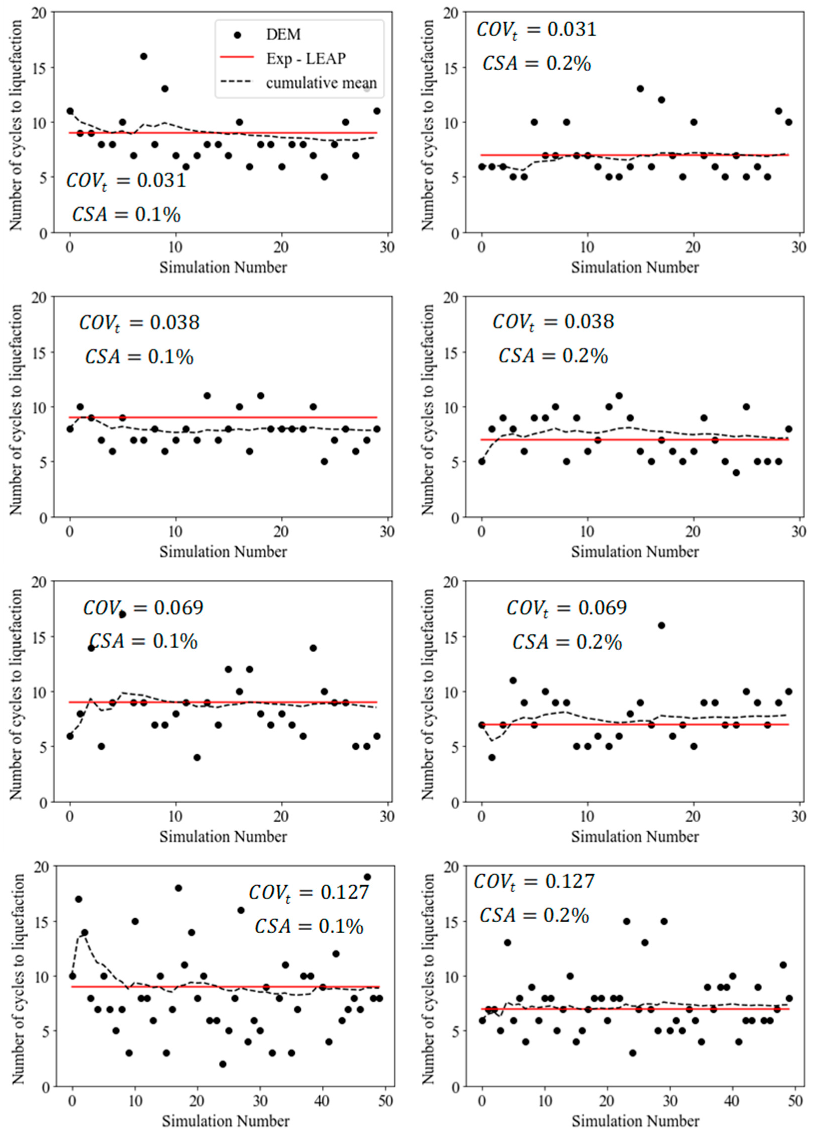
• The dispersion of the particle size distribution strongly affects the number of cycles to liquefaction; an average dispersion of finer up to 10% can result in a coefficient of variation of about 60% on the failure condition.
• Large uncertainties in the degrading behavior also occur when the initial dispersion on the particle size distribution is small; this can be linked to the variation in the minimum and maximum void ratio determining the variability in the relative density for each sample as well as the inherent anisotropy of the initial distribution of particles, as observed by Otsubo et al. [95].
• The distribution of the particle size strongly affects the liquefaction resistance because of the variation in the stress transmission between particles (see, e.g., [96,97]).
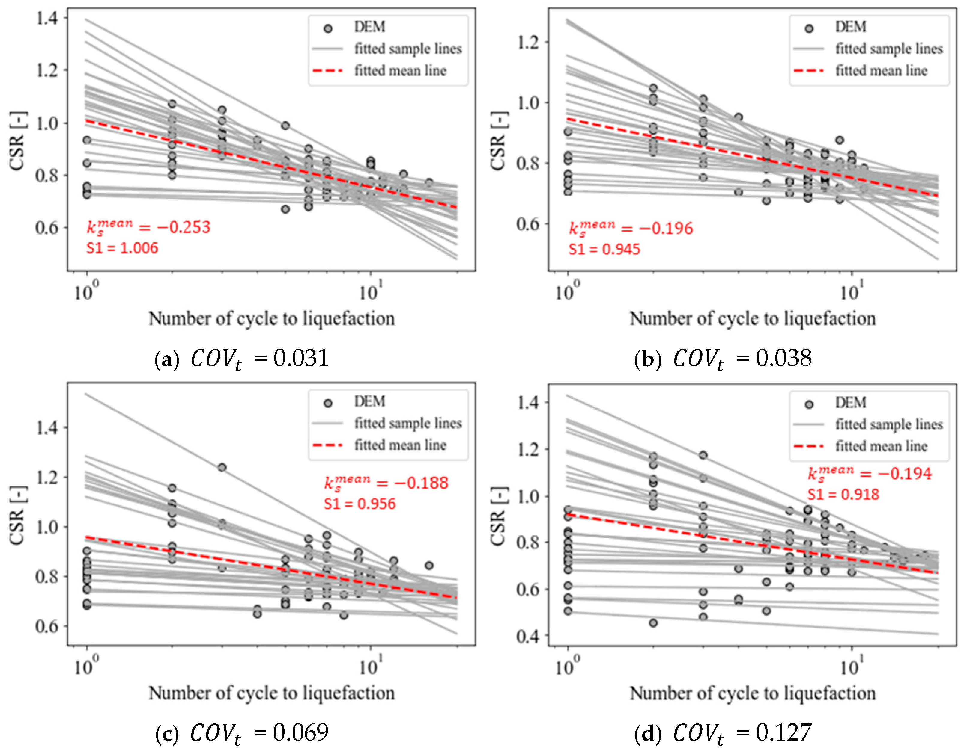
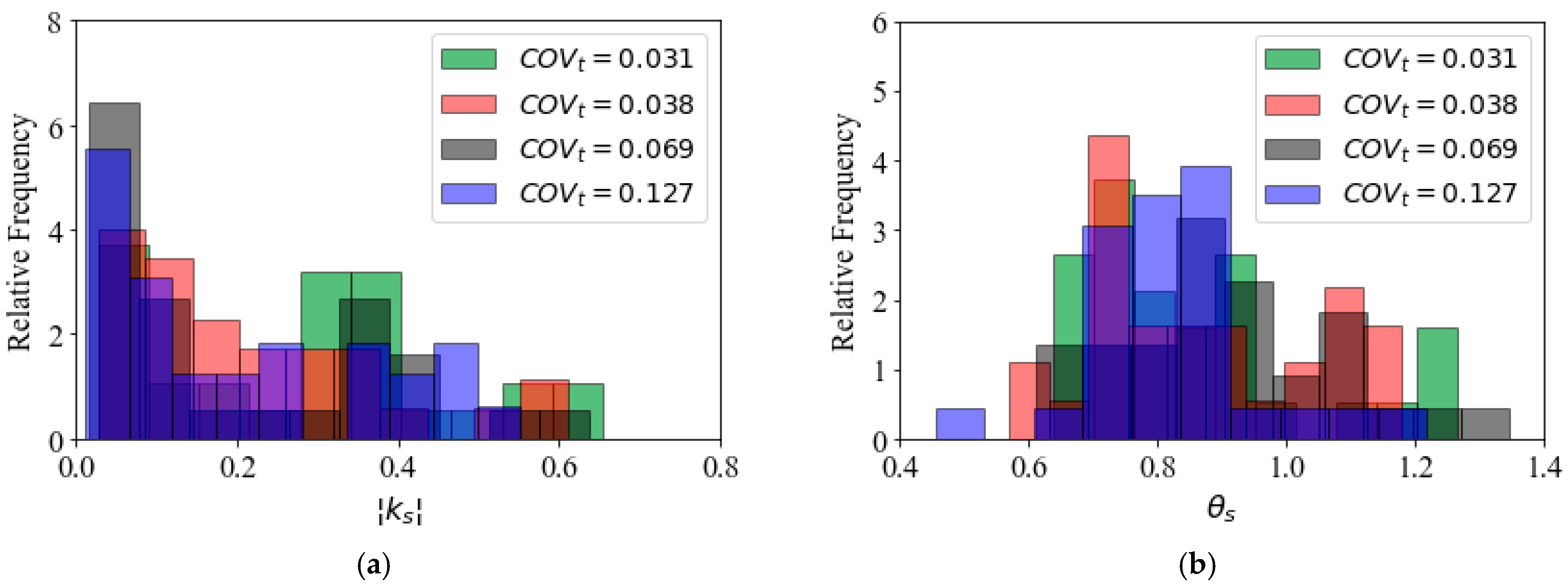
• Because of the large nonlinearities involved during cyclic soil behavior, the soil fatigue model parameters are not normally distributed, even when the initial distribution of the parameters is Gaussian.
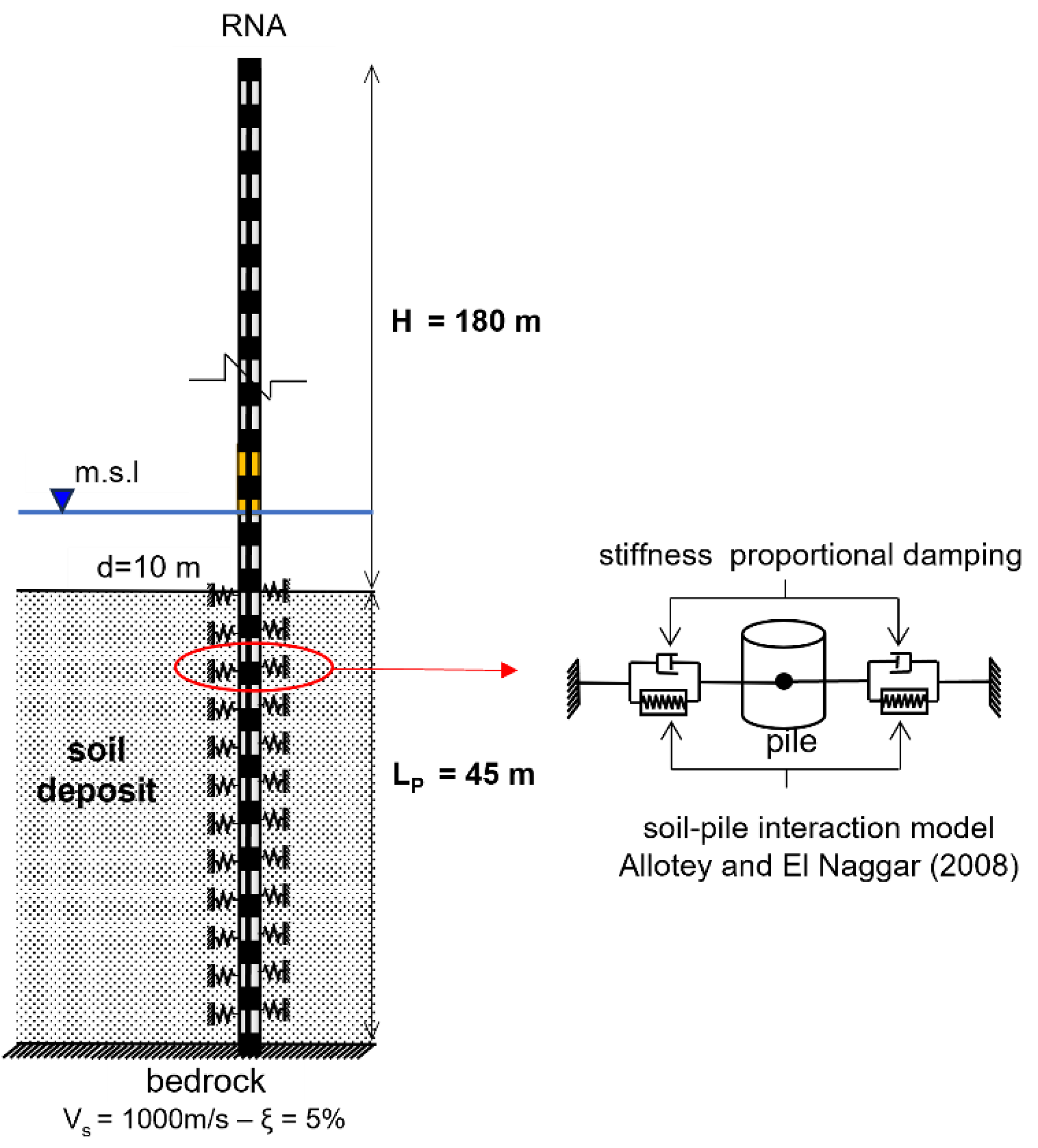
• The seismic analysis has shown an important effect of soil degradation on wind tower behavior; whilst the maximum bending moment and the fatigue on the tower wall is reduced compared to non-degrading soils, as observed in [10], the soil capacity is largely reduced, reducing the structural reliability of the wind turbine.

The proposed method is a viable tool for generating random soil parameters for fatigue and liquefaction models, which can be used in Monte Carlo simulation (MCS) reliability analyses or data-driven reliability approaches, e.g., [36,89,98].

References

1. Liu, Y.; Fu, Y.; Huang, L.; Zhang, K. Reborn and upgrading: Optimum repowering planning for offshore wind farms. Energy Rep. 2022, 8, 5204–5214. [Google Scholar] [CrossRef]
2. Mardfekri, M.; Gardoni, P.; Bisadi, V. Service reliability of offshore wind turbines. Int. J. Sustain. Energy 2015, 34, 468–484. [Google Scholar] [CrossRef]
3. Zorzi, G.; Mankar, A.; Velarde, J.; Sørensen, J.D.; Arnold, P.; Kirsch, F. Reliability analysis of offshore wind turbine foundations under lateral cyclic loading. Wind Energy Sci. 2020, 5, 1521–1535. [Google Scholar] [CrossRef]
4. Yu, Y.; Chen, X.; Guo, Z.; Zhang, J.; Lü, Q. Robust design of monopiles for offshore wind turbines considering uncertainties in dynamic loads and soil parameters. Ocean. Eng. 2022, 266, 112822. [Google Scholar] [CrossRef]
5. Johari, A.; Javadi, A.A.; Makiabadi, M.H.; Khodaparast, A.R. Reliability assessment of liquefaction potential using the jointly distributed random variables method. Soil Dyn. Earthq. Eng. 2012, 38, 81–87. [Google Scholar] [CrossRef]
6. Johari, A.; Pour, J.R.; Javadi, A. Reliability analysis of static liquefaction of loose sand using the random finite element method. Eng. Comput. 2015, 32, 2100–2119. [Google Scholar] [CrossRef]
7. Johari, A.; Khodaparast, A.R.; Javadi, A.A. An Analytical Approach to Probabilistic Modeling of Liquefaction Based on Shear Wave Velocity. Iran J. Sci. Technol. Trans. Civ. Eng. 2019, 43, 263–275. [Google Scholar] [CrossRef]
8. Phoon, K.-K.; Kulhawy, F.H. Characterization of geotechnical variability. Can. Geotech. J. 1999, 36, 612–624. [Google Scholar] [CrossRef]
9. Manolis, G.D. Stochastic soil dynamics. Soil Dyn. Earthq. Eng. 2002, 22, 3–15. [Google Scholar] [CrossRef]
10. Schafhirt, S.; Page, A.; Eiksund, G.R.; Muskulus, M. Influence of Soil Parameters on the Fatigue Lifetime of Offshore Wind Turbines with Monopile Support Structure. Energy Procedia 2016, 94, 347–356. [Google Scholar] [CrossRef]
11. Damgaard, M.; Bayat, M.; Andersen, L.V.; Ibsen, L.B. Assessment of the dynamic behaviour of saturated soil subjected to cyclic loading from offshore monopile wind turbine foundations. Comput. Geotech. 2014, 61, 116–126. [Google Scholar] [CrossRef]
12. Damgaard, M.; Andersen, L.V.; Ibsen, L.B. Dynamic response sensitivity of an offshore wind turbine for varying subsoil conditions. Ocean. Eng. 2015, 101, 227–234. [Google Scholar] [CrossRef]
13. Damgaard, M.; Andersen, L.V.; Ibsen, L.B.; Toft, H.S.; Sørensen, J.D. A probabilistic analysis of the dynamic response of monopile foundations: Soil variability and its consequences. Probabilistic Eng. Mech. 2015, 41, 46–59. [Google Scholar] [CrossRef]
14. Kementzetzidis, E.; Metrikine, A.V.; Versteijlen, W.G.; Pisanò, F. Frequency effects in the dynamic lateral stiffness of monopiles in sand: Insight from field tests and 3D FE modelling. Géotechnique 2021, 71, 812–825. [Google Scholar] [CrossRef]
15. Yeter, B.; Garbatov, Y.; Guedes Soares, C. Uncertainty analysis of soil-pile interactions of monopile offshore wind turbine support structures. Appl. Ocean. Res. 2019, 82, 74–88. [Google Scholar] [CrossRef]
16. Stuyts, B.; Weijtjens, W.; Gkougkoudi-Papaioannou, M.; Devriendt, C.; Troch, P.; Kheffache, A. Insights from in-situ pore pressure monitoring around a wind turbine monopile. Ocean. Eng. 2023, 269, 113556. [Google Scholar] [CrossRef]
17. Sun, Y.; Xu, C.; Naggar, M.H.E.; Du, X.; Dou, P. Cumulative cyclic response of offshore monopile in sands. Appl. Ocean. Res. 2023, 133, 103481. [Google Scholar] [CrossRef]
18. Sun, Y.; Xu, C.; Cui, C.; Naggar, M.H.E.; Du, X. Seismic Response of Monopile-Supported OWT Structure Considering Effect of Long-Term Cyclic Loading. Int. J. Str. Stab. Dyn. 2023, 23, 2350099. [Google Scholar] [CrossRef]
19. Shajarati, A.; Sørensen, K.W.; Nielsen, S.K.; Ibsen, L.B. Behaviour of Cohesionless Soils During Cyclic Loading; DCE Technical Memorandum No. 14; Aalborg University: Aalborg, Denmark, 2012. [Google Scholar]
20. Zienkiewicz, O.C.; Shiomi, T. Dynamic behaviour of saturated porous media; The generalized Biot formulation and its numerical solution. Num. Anal. Meth. Geomech. 1984, 8, 71–96. [Google Scholar] [CrossRef]
21. Esfeh, P.K.; Kaynia, A.M. Numerical modeling of liquefaction and its impact on anchor piles for floating offshore structures. Soil Dyn. Earthq. Eng. 2019, 127, 105839. [Google Scholar] [CrossRef]
22. Kementzetzidis, E.; Corciulo, S.; Versteijlen, W.G.; Pisanò, F. Geotechnical aspects of offshore wind turbine dynamics from 3D non-linear soil-structure simulations. Soil Dyn. Earthq. Eng. 2019, 120, 181–199. [Google Scholar] [CrossRef]
23. Kumari, S.; Sawant, V.A. Numerical simulation of liquefaction phenomenon considering infinite boundary. Soil Dyn. Earthq. Eng. 2021, 142, 106556. [Google Scholar] [CrossRef]
24. Idriss, I.M.; Dobry, R.; Singh, R.D. Nonlinear Behavior of Soft Clays during Cyclic Loading. J. Geotech. Engrg. Div. 1978, 104, 1427–1447. [Google Scholar] [CrossRef]
25. Matlock, H. SPASM 8—A Dynamic Beam-Column Program for Seismic Pile Analysis with Support Motion; Fugro Inc.: Long Beach, CA, USA, 1979. [Google Scholar]
26. Allotey, N.; El Naggar, M.H. A Consistent Soil Fatigue Framework Based on the Number of Equivalent Cycles. Geotech. Geol. Eng. 2008, 26, 65–77. [Google Scholar] [CrossRef]
27. Nikitas, G.; Arany, L.; Aingaran, S.; Vimalan, J.; Bhattacharya, S. Predicting long term performance of offshore wind turbines using cyclic simple shear apparatus. Soil Dyn. Earthq. Eng. 2017, 92, 678–683. [Google Scholar] [CrossRef]
28. Tsai, C.-C. Generalized simple model for predicting the modulus degradation and strain accumulation of clay subject to long-term undrained cyclic loading. Ocean. Eng. 2022, 254, 111412. [Google Scholar] [CrossRef]
29. Prevost, J.H. DYNAFLOW; Version 98, Release 02. A.; Princeton University, Department of Civil Engineering & Op. Res.: Princeton, NJ, USA, 1998. [Google Scholar]
30. Ziotopoulou, K.; Boulanger, R.W. Calibration and implementation of a sand plasticity plane-strain model for earthquake engineering applications. Soil Dyn. Earthq. Eng. 2013, 53, 268–280. [Google Scholar] [CrossRef]
31. Beaty, M.H. Application of UBCSAND to the LEAP centrifuge experiments. Soil Dyn. Earthq. Eng. 2018, 104, 143–153. [Google Scholar] [CrossRef]
32. Ghofrani, A.; Arduino, P. Prediction of LEAP centrifuge test results using a pressure-dependent bounding surface constitutive model. Soil Dyn. Earthq. Eng. 2018, 113, 758–770. [Google Scholar] [CrossRef]
33. Mardfekri, M.; Gardoni, P. Multi-hazard reliability assessment of offshore wind turbines: Multi-hazard reliability assessment of offshore wind turbines. Wind Energy 2015, 18, 1433–1450. [Google Scholar] [CrossRef]
34. Tombari, A.; Stefanini, L. Hybrid fuzzy–stochastic 1D site response analysis accounting for soil uncertainties. Mech. Syst. Signal Process. 2019, 132, 102–121. [Google Scholar] [CrossRef]
35. Andersen, K.H.; Engin, H.K.; D’Ignazio, M.; Yang, S. Determination of cyclic soil parameters for offshore foundation design from an existing data base. Ocean. Eng. 2023, 267, 113180. [Google Scholar] [CrossRef]
36. Tombari, A.; Dobbs, M.; Holland, L.M.J.; Stefanini, L. A rigorous possibility approach for the geotechnical reliability assessment supported by external database and local experience. Comput. Geotech. 2024, 166, 105967. [Google Scholar] [CrossRef]
37. Maksimov, F.; Tombari, A. Derivation of Cyclic Stiffness and Strength Degradation Curves of Sands through Discrete Element Modelling. Modelling 2022, 3, 400–416. [Google Scholar] [CrossRef]
38. Cundall, P.A.; Strack, O.D.L. A discrete numerical model for granular assemblies. Géotechnique 1979, 29, 47–65. [Google Scholar] [CrossRef]
39. Kozicki, J.; Tejchman, J.; Mühlhaus, H. Discrete simulations of a triaxial compression test for sand by DEM. Num. Anal. Meth. Geomech. 2014, 38, 1923–1952. [Google Scholar] [CrossRef]
40. Thornton, C.; Liu, L. DEM simulations of uni-axial compression and decompression. Compact. Soils Granulates Powders 2000, 2, 251–261. [Google Scholar]
41. Lee, S.J.; Hashash, Y.M.A.; Nezami, E.G. Simulation of triaxial compression tests with polyhedral discrete elements. Comput. Geotech. 2012, 43, 92–100. [Google Scholar] [CrossRef]
42. De Bono, J.P.; McDowell, G.R. DEM of triaxial tests on crushable sand. Granular Matter 2014, 16, 551–562. [Google Scholar] [CrossRef]
43. Zorzi, G.; Kirsch, F.; Gabrieli, F.; Rackwitz, F. Long-Term Cyclic Triaxial Tests with Dem Simulations. In Proceedings of the V International Conference on Particle-Based Methods—Fundamentals and Applications, Hannover, Germany, 26–28 October 2017. [Google Scholar]
44. Ali, U.; Kikumoto, M.; Ciantia, M. Impact of particle elongation on the behavior of round and angular granular media: Consequences of particle rotation and force chain development. Comput. Geotech. 2024, 165, 105858. [Google Scholar] [CrossRef]
45. Wang, X.; Xu, C.; Liang, K.; Iqbal, K. Mechanical characteristics and microstructure of saturated sand under monotonic and cyclic loading conditions. Soil Dyn. Earthq. Eng. 2024, 176, 108283. [Google Scholar] [CrossRef]
46. Sitharam, T.G. Discrete element modelling of cyclic behaviour of granular materials. Geotech. Geol. Eng. 2003, 21, 297–329. [Google Scholar] [CrossRef]
47. O’Sullivan, C.; Cui, L.; O’Neill, S.C. Discrete Element Analysis of the Response of Granular Materials During Cyclic Loading. S&F 2008, 48, 511–530. [Google Scholar] [CrossRef]
48. Zhang, L.; Evans, T.M. Boundary effects in discrete element method modeling of undrained cyclic triaxial and simple shear element tests. Granular Matter 2018, 20, 60. [Google Scholar] [CrossRef]
49. Martin, E.L.; Thornton, C.; Utili, S. Micromechanical investigation of liquefaction of granular media by cyclic 3D DEM tests. Géotechnique 2020, 70, 906–915. [Google Scholar] [CrossRef]
50. Wu, Q.X.; Pan, K.; Yang, Z.X. Undrained cyclic behavior of granular materials considering initial static shear effect: Insights from discrete element modeling. Soil Dyn. Earthq. Eng. 2021, 143, 106597. [Google Scholar] [CrossRef]
51. Cui, L.; Bhattacharya, S. Soil–monopile interactions for offshore wind turbines. Proc. Inst. Civ. Eng.- Eng. Comput. Mech. 2016, 169, 171–182. [Google Scholar] [CrossRef]
52. Sharif, Y.U.; Brown, M.J.; Ciantia, M.O.; Cerfontaine, B.; Davidson, C.; Knappett, J.; Meijer, G.J.; Ball, J. Using discrete element method (DEM) to create a cone penetration test (CPT)-based method to estimate the installation requirements of rotary-installed piles in sand. Can. Geotech. J. 2021, 58, 919–935. [Google Scholar] [CrossRef]
53. Cerfontaine, B.; Ciantia, M.O.; Brown, M.J.; White, D.J.; Sharif, Y.U. DEM study of particle scale effect on plain and rotary jacked pile behaviour in granular materials. Comput. Geotech. 2023, 161, 105559. [Google Scholar] [CrossRef]
54. Li, L.; Zheng, M.; Liu, X.; Wu, W.; Liu, H.; El Naggar, M.H.; Jiang, G. Numerical analysis of the cyclic loading behavior of monopile and hybrid pile foundation. Comput. Geotech. 2022, 144, 104635. [Google Scholar] [CrossRef]
55. Vasko, A. An Investigation into the Behavior of Ottawa Sand Through Monotonic and Cyclic Shear Tests. Master’s Thesis, The George Washington University, Washington, DC, USA, 2015. [Google Scholar]
56. ElGhoraiby, M.A.; Park, H.; Manzari, M.T. Stress-strain behavior and liquefaction strength characteristics of Ottawa F65 sand. Soil Dyn. Earthq. Eng. 2020, 138, 106292. [Google Scholar] [CrossRef]
57. Sobieski, W.; Lipiński, S. The influence of particle size distribution on parameters characterizing the spatial structure of porous beds. Granular Matter 2019, 21, 14. [Google Scholar] [CrossRef]
58. Winkler, E. Die Lehre von der Elastizitat und Festigkeit; Verlag von H. Dominicus: Prague, Czech Republic, 1876. [Google Scholar]
59. Allotey, N.; El Naggar, M.H. Generalized dynamic Winkler model for nonlinear soil–structure interaction analysis. Can. Geotech. J. 2008, 45, 560–573. [Google Scholar] [CrossRef]
60. Choobbasti, A.J.; Zahmatkesh, A. Computation of degradation factors of p-y curves in liquefiable soils for analysis of piles using three-dimensional finite-element model. Soil Dyn. Earthq. Eng. 2016, 89, 61–74. [Google Scholar] [CrossRef]
61. Heidari, M.; Jahanandish, M.; El Naggar, H.; Ghahramani, A. Nonlinear cyclic behavior of laterally loaded pile in cohesive soil. Can. Geotech. J. 2014, 51, 129–143. [Google Scholar] [CrossRef]
62. Heidari, M.; El Naggar, H.; Jahanandish, M.; Ghahramani, A. Generalized cyclic p–y curve modeling for analysis of laterally loaded piles. Soil Dyn. Earthq. Eng. 2014, 63, 138–149. [Google Scholar] [CrossRef]
63. Tsai, C.-C.; Li, Y.-P.; Lin, S.-H. p-y based approach to predicting the response of monopile embedded in soft clay under long-term cyclic loading. Ocean. Eng. 2023, 275, 114144. [Google Scholar] [CrossRef]
64. White, D.J.; Doherty, J.P.; Guevara, M.; Watson, P.G. A cyclic p-y model for the whole-life response of piles in soft clay. Comput. Geotech. 2022, 141, 104519. [Google Scholar] [CrossRef]
65. Zeng, F.; Jiang, C.; Liu, P. Cyclic p-y curve model of piles subjected to two-way load considering the collapse and densification of sand. Ocean. Eng. 2023, 289, 116122. [Google Scholar] [CrossRef]
66. Xiao-Ling, Z.; Rui, Z.; Yan, H. Study on p-y curve of large diameter pile under long-term cyclic loading. Appl. Ocean. Res. 2023, 140, 103736. [Google Scholar] [CrossRef]
67. Byrne, B.W.; Houlsby, G.T.; Burd, H.J.; Gavin, K.G.; Igoe, D.J.P.; Jardine, R.J.; Martin, C.M.; McAdam, R.A.; Potts, D.M.; Taborda, D.M.G.; et al. PISA design model for monopiles for offshore wind turbines: Application to a stiff glacial clay till. Géotechnique 2020, 70, 1030–1047. [Google Scholar] [CrossRef]
68. Cao, G.; Ding, X.; Yin, Z.; Zhou, H.; Zhou, P. A new soil reaction model for large-diameter monopiles in clay. Comput. Geotech. 2021, 137, 104311. [Google Scholar] [CrossRef]
69. Heidari, M.; Hesham El Naggar, M. Analytical Approach for Seismic Performance of Extended Pile-Shafts. J. Bridge Eng. 2018, 23, 04018069. [Google Scholar] [CrossRef]
70. Matlock, H. Correlation for Design of Laterally Loaded Piles in Soft Clay. In Proceedings of the Offshore Technology Conference, Houston, TX, USA, 22–24 April 1970. [Google Scholar] [CrossRef]
71. Wang, L.; Lai, Y.; Hong, Y.; Mašín, D. A unified lateral soil reaction model for monopiles in soft clay considering various length-to-diameter (L/D) ratios. Ocean. Eng. 2020, 212, 107492. [Google Scholar] [CrossRef]
72. Plassiard, J.-P.; Belheine, N.; Donzé, F.-V. A spherical discrete element model: Calibration procedure and incremental response. Granular Matter 2009, 11, 293–306. [Google Scholar] [CrossRef]
73. Fukumoto, Y.; Sakaguchi, H.; Murakami, A. The role of rolling friction in granular packing. Granular Matter 2013, 15, 175–182. [Google Scholar] [CrossRef]
74. Barnett, N.; Rahman, M.M.; Karim, M.R.; Nguyen, H.B.K. Evaluating the particle rolling effect on the characteristic features of granular material under the critical state soil mechanics framework. Granular Matter 2020, 22, 89. [Google Scholar] [CrossRef]
75. Li, Z.; Zeng, X.; Wen, T.; Zhang, Y. Numerical Comparison of Contact Force Models in the Discrete Element Method. Aerospace 2022, 9, 737. [Google Scholar] [CrossRef]
76. Van Gunsteren, W.F.; Berendsen, H.J.C. A Leap-frog Algorithm for Stochastic Dynamics. Mol. Simul. 1988, 1, 173–185. [Google Scholar] [CrossRef]
77. Grubmüller, H.; Heller, H.; Windemuth, A.; Schulten, K. Generalized Verlet algorithm for efficient molecular dynamics simulations with long-range interactions. Mol. Simul. 1991, 6, 121–142. [Google Scholar] [CrossRef]
78. Kuhn, M.R.; Renken, H.E.; Mixsell, A.D.; Kramer, S.L. Investigation of Cyclic Liquefaction with Discrete Element Simulations. J. Geotech. Geoenviron. Eng. 2014, 140, 04014075. [Google Scholar] [CrossRef]
79. El Shamy, U.; Zeghal, M. Coupled Continuum-Discrete Model for Saturated Granular Soils. J. Eng. Mech. 2005, 131, 413–426. [Google Scholar] [CrossRef]
80. Kutter, B.L.; Manzari, M.T.; Zeghal, M. (Eds.) Model Tests and Numerical Simulations of Liquefaction and Lateral Spreading: LEAP-UCD-2017; Springer International Publishing: Cham, Switzerland, 2020. [Google Scholar] [CrossRef]
81. Radjai, F.; Dubois, F. Discrete-Element Modeling of Granular Materials; Wiley-Iste: London, UK, 2011. [Google Scholar]
82. Hosn, R.A.; Sibille, L.; Benahmed, N.; Chareyre, B. Discrete numerical modeling of loose soil with spherical particles and interparticle rolling friction. Granular Matter 2017, 19, 1–12. [Google Scholar]
83. Morris, M.D. Factorial Sampling Plans for Preliminary Computational Experiments. Technometrics 1991, 33, 161–174. [Google Scholar] [CrossRef]
84. Saltelli, A.; Ratto, M.; Andres, T.; Campolongo, F.; Cariboni, J.; Gatelli, D.; Saisana, M.; Tarantola, S. Global Sensitivity Analysis. The Primer, 1st ed.; Wiley: Hoboken, NJ, USA, 2007. [Google Scholar] [CrossRef]
85. Kumar, S.S.; Krishna, A.M.; Dey, A. Assessment of Dynamic Response of Cohesionless Soil Using Strain-Controlled and Stress-Controlled Cyclic Triaxial Tests. Geotech. Geol. Eng. 2020, 38, 1431–1450. [Google Scholar] [CrossRef]
86. Schneider, J.A.; Moss, R.E.S. Linking cyclic stress and cyclic strain based methods for assessment of cyclic liquefaction triggering in sands. Géotechnique Lett. 2011, 1, 31–36. [Google Scholar] [CrossRef]
87. DeAlba, P.; Seed, H.B.; Chan, C.K. Sand Liquefaction in Large-Scale Simple Shear Tests. J. Geotech. Eng. Div. ASCE 1976, 102, 909–927. [Google Scholar] [CrossRef]
88. Zhao, X.; Zhu, J.; Wu, Y.; Jia, Y.; Bur, N.; Colliat, J.B.; Bian, H. Experimental Study and DEM Simulation of Size Effects on the Dry Density of Rockfill Material. Front. Phys. 2022, 10, 837727. [Google Scholar] [CrossRef]
89. Tombari, A.; Stefanini, L.; Nicosia, G.L.D.; Holland, L.M.J.; Dobbs, M. Geotechnical data-driven possibility reliability assessment. Comput. Geotech. 2025, 185, 107311. [Google Scholar] [CrossRef]
90. Gaertner, E.; Rinker, J.; Sethuraman, L.; Zahle, F.; Anderson, B.; Barter, G.; Abbas, N.; Meng, F.; Bortolotti, P.; Skrzypinski, W.; et al. Definition of the IEA 15-Megawatt Offshore Reference Wind Turbine; International Energy Agency: Paris, France, 2020. Available online: https://www.nrel.gov/docs/fy20osti/75698.pdf (accessed on 1 May 2025).
91. Seismosoft. SeismoStruct 2025—Verification Report. 2025. Available online: https://seismosoft.com/wp-content/uploads/prods/lib/SeismoStruct-2025-User-Manual_ENG.pdf (accessed on 1 June 2025).
92. Tombari, A.; El Naggar, M.H.; Dezi, F. Impact of ground motion duration and soil non-linearity on the seismic performance of single piles. Soil Dyn. Earthq. Eng. 2017, 100, 72–87. [Google Scholar] [CrossRef]
93. Ragan, P.; Manuel, L. Comparing Estimates of Wind Turbine Fatigue Loads Using Time-Domain and Spectral Methods. Wind. Eng. 2007, 31, 83–99. [Google Scholar] [CrossRef]
94. Velarde, J.; Kramhøft, C.; Sørensen, J.D.; Zorzi, G. Fatigue reliability of large monopiles for offshore wind turbines. Int. J. Fatigue 2020, 134, 105487. [Google Scholar] [CrossRef]
95. Otsubo, M.; Chitravel, S.; Kuwano, R.; Hanley, K.J.; Kyokawa, H.; Koseki, J. Linking inherent anisotropy with liquefaction phenomena of granular materials by means of DEM analysis. Soils Found. 2022, 62, 101202. [Google Scholar] [CrossRef]
96. Mutabaruka, P.; Taiebat, M.; Pellenq, R.J.-M.; Radjai, F. Effects of size polydispersity on random close-packed configurations of spherical particles. Phys. Rev. E 2019, 100, 042906. [Google Scholar] [CrossRef]
97. Banerjee, S.K.; Yang, M.; Taiebat, M. Effect of coefficient of uniformity on cyclic liquefaction resistance of granular materials. Comput. Geotech. 2023, 155, 105232. [Google Scholar] [CrossRef]
98. Ching, J.; Wu, S.; Phoon, K.-K. Constructing Quasi-Site-Specific Multivariate Probability Distribution Using Hierarchical Bayesian Model. J. Eng. Mech. 2021, 147, 04021069. [Google Scholar] [CrossRef]
Figure 1. Three-step procedure to perform cyclic undrained triaxial testing on random samples generated through the Discrete Element Method [38], consisting of Step (1), random sample preparation, Step (2), isotropic consolidation, and Step (3), cyclic testing for each of the generated sample.
Jmse 13 01145 g001
Figure 2. Contact forces generated acting on the contact point between two touching particles.
Jmse 13 01145 g002
Figure 3. Generated sample using Equation (3) with C O V = 0 for (a) deterministic analysis, and (b) realizations generated with low C O V = 0.005 for inspecting the repeatability of the results.
Jmse 13 01145 g003
Figure 4. Cyclic response of a randomly generated sample with different (a) values of particle density and (b) number of particles considering a confining pressure of 200 kPa and a void ratio of 0.604.
Jmse 13 01145 g004
Figure 5. Ranking of the model parameters for (a) 5 model parameters and C S A = 0.4%, and (b) 4 parameters and C S A = 0.1%.
Jmse 13 01145 g005
Figure 6. Calibration and validation of the Ottawa F65 sand DEM model conducted at confining pressure of (a) 100 kPa and (b) 200 kPa for samples with a void ratio of 0.608.
Jmse 13 01145 g006
Figure 7. Comparison to experimental testing: (a) stress–strain hysteresis cycles, and (b) evolution of the mean stress.
Jmse 13 01145 g007
Figure 8. Failure condition curves obtained at two confining pressures, (a) 100 kPa and (b) 200 kPa.
Jmse 13 01145 g008
Figure 9. Strength degradation curves for several cyclic strain amplitudes conducted at a confining pressure of 100 kPa.
Jmse 13 01145 g009
Figure 10. Strength degradation curves for several cyclic strain amplitudes conducted at a confining pressure of 200 kPa.
Jmse 13 01145 g010
Figure 11. Particle size distribution functions of samples generated with (a) C O V t = 0.031 and (b) C O V t = 0.127 .
Jmse 13 01145 g011
Figure 12. Results of the Monte Carlo simulation in terms of the number of cycles to liquefaction for different C O V t and CSA values.
Jmse 13 01145 g012
Figure 13. Fatigue curves considering soil uncertainty for (ad) different COVs of the particle size distribution functions.
Jmse 13 01145 g013
Figure 14. Damage evolution curves from the randomly generated samples using C O V t = 0.069 for three levels of cyclic strain ratios, (a) C S A = 0.1 % , (b) C S A = 0.2 % , and (c) C S A = 0.4 % .
Jmse 13 01145 g014
Figure 15. Histogram plots of the distributions of (a) the fatigue curve slope parameter and (b) the shape factor at C S A = 0.2 % .
Jmse 13 01145 g015
Figure 16. Schematic of the finite element model of the IEA 15 MW reference wind turbine [59].
Jmse 13 01145 g016
Figure 17. Earthquakes events considered in this study: (a) scaled acceleration time-histories and (b) distribution of the equivalent number of cycles for the San Fernando 1971 and Imperial Valley 1979 events.
Jmse 13 01145 g017
Figure 18. Bending moment envelopes resulting from the (a) San Fernando 1971 earthquake and (b) Imperial Valley 1979 event.
Jmse 13 01145 g018
Figure 19. Distribution of the normalized damage equivalent load related to the peak bending moment obtained from the short- and long-term-duration events.
Jmse 13 01145 g019