Adaptive Event-Triggered Predictive Control for Agile Motion of Underwater Vehicles

Abstract

As the demand for underwater robots in complex environments continues to grow, research on their agile motion capabilities becomes increasingly crucial. This paper focuses on the design and agile motion control of autonomous underwater vehicles (AUVs) operating in subsea environments, addressing key issues such as structural design, system modeling, and control algorithm development. An optimization model for the arrangement of propellers is formulated and solved using a Sequential Quadratic Programming (SQP) algorithm. Computational Fluid Dynamics (CFD) software is employed for hydrodynamic analysis and shape optimization. A novel adaptive event-triggered nonlinear model predictive control (AET-NMPC) algorithm is proposed and compared with traditional Cascaded Proportional–Integral–Derivative (PID) control and event-triggered cascaded PID control algorithms. Simulation and experimental results demonstrate that the AET-NMPC algorithm significantly enhances the response capability and control accuracy of underwater robots in complex tasks, with the trajectory tracking error being reduced to 4.89%. This study provides valuable insights into the design and control strategies for AUVs, paving the way for more sophisticated underwater operations in challenging environments.

1. Introduction

Autonomous underwater vehicles (AUVs) have become indispensable tools in a wide spectrum of underwater applications, including oceanographic exploration, environmental monitoring, infrastructure inspection, and search-and-rescue missions [1,2,3,4]. AUV performance is often constrained by the inherent trade-off between hydrodynamic efficiency and maneuverability [5,6]. Traditional torpedo-shaped AUV designs (e.g., REMUS and Bluefin) are optimized for endurance and low drag, enabling long-range missions. However, these vehicles exhibit limited agility and control authority, especially in confined, cluttered, or dynamically changing environments [7,8].

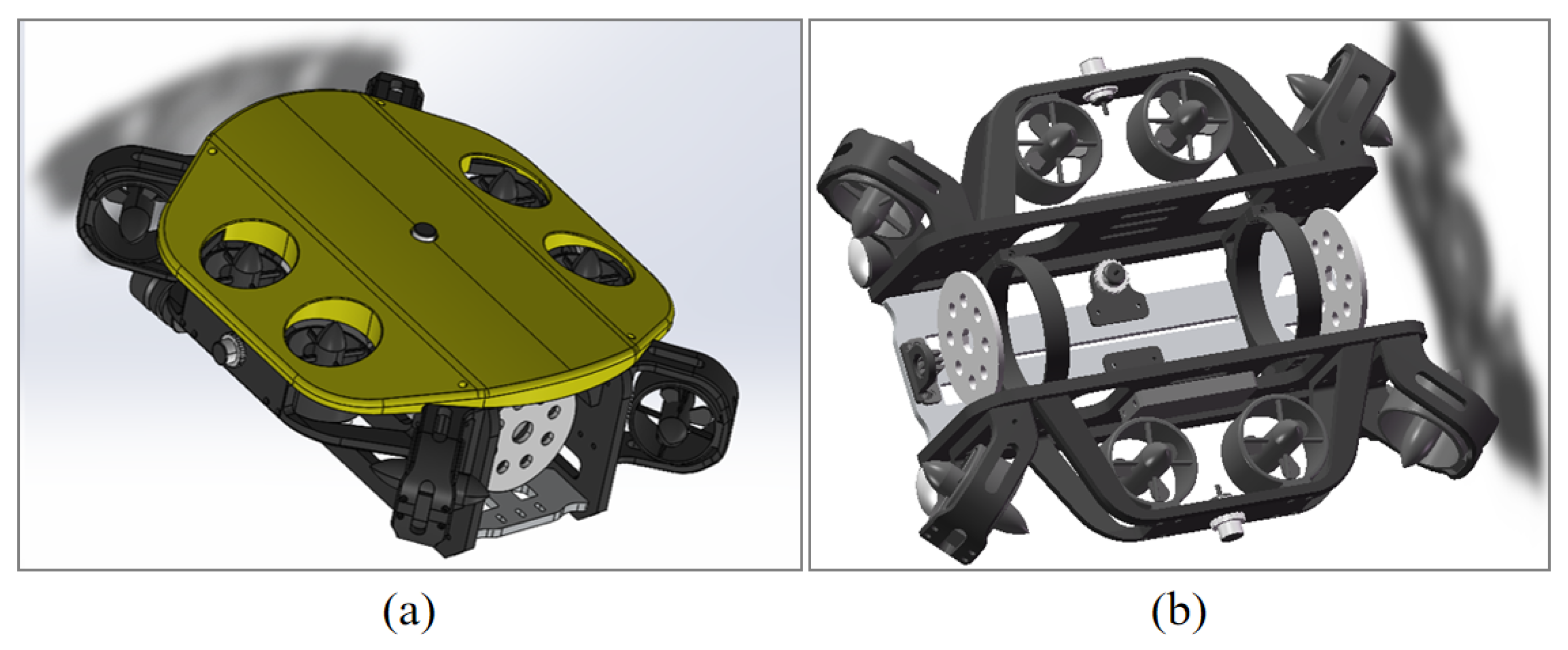
In contrast, AUVs designed for seabed operations prioritize compactness, stability, and precise maneuverability over long-range efficiency. These vehicles often feature non-streamlined, boxy configurations and multiple thrusters with 6-DOF actuation, offering superior position control and agility in complex terrains (Figure 1). However, such designs typically suffer from increased drag, reduced speed, and limited endurance, making them less suitable for large-scale or high-speed missions. For seabed AUVs, stability, maneuverability, and responsiveness are of paramount importance. While hydrodynamic optimization can improve endurance and speed to some extent, the nonlinear, time-varying nature of underwater dynamics—combined with unpredictable environmental disturbances such as ocean currents and turbulence—poses significant challenges for motion control [9,10].

Classical control strategies, including PID and LQR, are widely used due to their simplicity and ease of implementation. However, these methods often lack robustness to model uncertainties, actuator nonlinearity, and external disturbances [11,12]. Advanced nonlinear control strategies, such as sliding mode control (SMC) [13], backstepping [14], and model predictive control (MPC) [15,16], have demonstrated improved tracking and disturbance rejection. Nevertheless, their practical deployment is often hindered by high computational costs and sensitivity to inaccurate hydrodynamic modeling. Moreover, many existing control frameworks ignore practical constraints such as thruster saturation, dead zones, and actuator faults, which can severely degrade control performance—particularly during aggressive maneuvers like sharp turning, docking, or disturbance rejection [17,18,19,20,21].

To address these challenges, this study proposes a novel agile AUV platform tailored for subsea operations, along with a hybrid control strategy that combines nonlinear model predictive control (NMPC) with an event-triggered PID framework. The main objectives of this research are to:

• Enhance the agility and trajectory tracking accuracy of the AUV;
• Accommodate real-world actuator constraints;
• Maintain control robustness in uncertain and dynamic underwater environments.

1.1. Related Work

In recent years, a variety of control techniques and AUV platforms have been proposed to tackle the issues of agility and robustness in underwater environments.

Table 1. Comparison of related work.

Method	AUV Type	Control Strategy	Constraints
SMC-Based AUV Control [13]	Torpedo shape	Sliding Mode Control	No
Backstepping for AUV [14]	Box type	Backstepping	No
MPC-Based Control [15]	Torpedo shape	Linear MPC	Limited (no dead-zone modeling)
Fault-Tolerant Control [18]	Box type	Adaptive + Fault Detection	Partial (faults only)
Event-Triggered PID [22]	Box type	Event-Triggered PID	No

presents a comparative overview of representative state-of-the-art approaches in terms of AUV design, control strategy, thruster constraint handling, and application domain.

As shown in Table 1, most existing studies have either focused on simplified control models that ignore actuator nonlinearities or applied computationally intensive algorithms unsuitable for real-time deployment. Very few studies have effectively combined advanced nonlinear control with practical constraint handling, especially in the context of agile seabed AUVs navigating in uncertain environments.

1.2. Innovation and Contributions

This research addresses the above limitations by integrating hydrodynamic optimization and a computationally efficient hybrid control framework with the following capabilities:

• Combines event-triggered PID for low-level fast response with nonlinear MPC for high-level prediction and constraint handling;
• Explicitly models thruster dead zones, saturation, and potential actuator faults;
• Is implemented on a custom-designed agile AUV platform with 6-DOF control and multi-thruster configuration for seabed operation;
• Is validated through both simulation and physical pool experiments, demonstrating enhanced agility, trajectory tracking accuracy, and robustness under disturbances.

By bridging the gap between advanced control theory and real-world underwater application, this study contributes a novel, practical, and robust control solution for agile AUVs operating in complex seabed environments. The rest of this paper is arranged as follows: The methodology part begins with the design and implementation of a subsea AUV, including thruster configuration, hardware integration, and software architecture to support agile motion control. Following this, a comprehensive hydrodynamic performance analysis is conducted to optimize the vehicle’s underwater behavior. To further enhance control performance, an adaptive event-triggered predictive control strategy is proposed, combining an event-triggered PID controller with a nonlinear model predictive control (NMPC) algorithm. The effectiveness of the proposed design and control methods is validated through a series of simulations and pool experiments. This study concludes that the integration of hydrodynamic optimization and advanced control algorithms significantly enhances the AUV’s agility and precision, making it well suited for underwater exploration and operational tasks in challenging terrain.

2. Design and Implementation of a Subsea AUV

This chapter provides a detailed overview of the design and implementation of the AUV, including the thruster layout, structural design, hardware platform configuration, and software system. By optimizing each design module, the AUV’s mobility, control accuracy, and efficiency are enhanced, ensuring its capability to perform complex tasks such as ocean exploration.

The mechanical design of the underwater AUV is formulated under the following key assumptions and constraints:

(1)

The AUV operates in a fully submerged condition with negligible wave effects;

(2)

Structural deformation is considered negligible under operational pressure;

(3)

Buoyancy and gravity centers remain constant during steady-state operation;

(4)

Fluid–structure interaction follows potential flow theory for added mass calculations.

The overall 3D model of the AUV is shown in Figure 2a. The structure of the entire underwater robot is made of HDPE material, with a hydrodynamic outer shell fabricated using photosensitive resin through 3D printing, and the sealed cabin is constructed from acrylic material. The outer shell primarily serves to protect the internal components of the underwater robot from the impact of ocean currents and debris, while also providing a streamlined shape that enhances hydrodynamic performance, reduces fluid resistance during operation, and thereby lowers power consumption.

The internal framework (Figure 2b) is a crucial structural component that supports and secures various parts inside the robot, such as the pressure-resistant cabin. During underwater maneuvers, it provides sufficient strength to keep all components tightly integrated, overcoming inertial forces and fluid resistance to maintain coordinated movement. The pressure-resistant cabin is designed to protect critical equipment such as batteries and control system hardware, and the designed working depth is 100 m. The parameters and constraints of the subsea AUV are given in

Table 2. Parameters and constraints of the subsea AUV.

(a)
Parameter	Value	Unit
Size	500 × 385 × 200	mm
Weight	8.5	kg
Thruster setting	4 horizontal, 4 vertical	/
Cruising speed	3	knot
(b)
Constraint	Content	Note
Maximum operational depth	100m	1 MPa pressure
Material yield strength	≥9.6 MPa	PMMA acrylic
Neutral buoyancy tolerance	±0.05 kg

a,b.

2.1. Thruster Configuration

The underwater robot designed in this study utilizes four horizontal thrusters and four vertical thrusters. The horizontal thrusters are responsible for generating thrust for horizontal movement and enable horizontal maneuvers such as zero turning radius rotation through differential control. The vertical thrusters provide thrust in the vertical direction, which is used to maintain the robot’s attitude during hovering, ensure a stable angle of attack during horizontal motion, and offer driving force for small-range vertical movements.

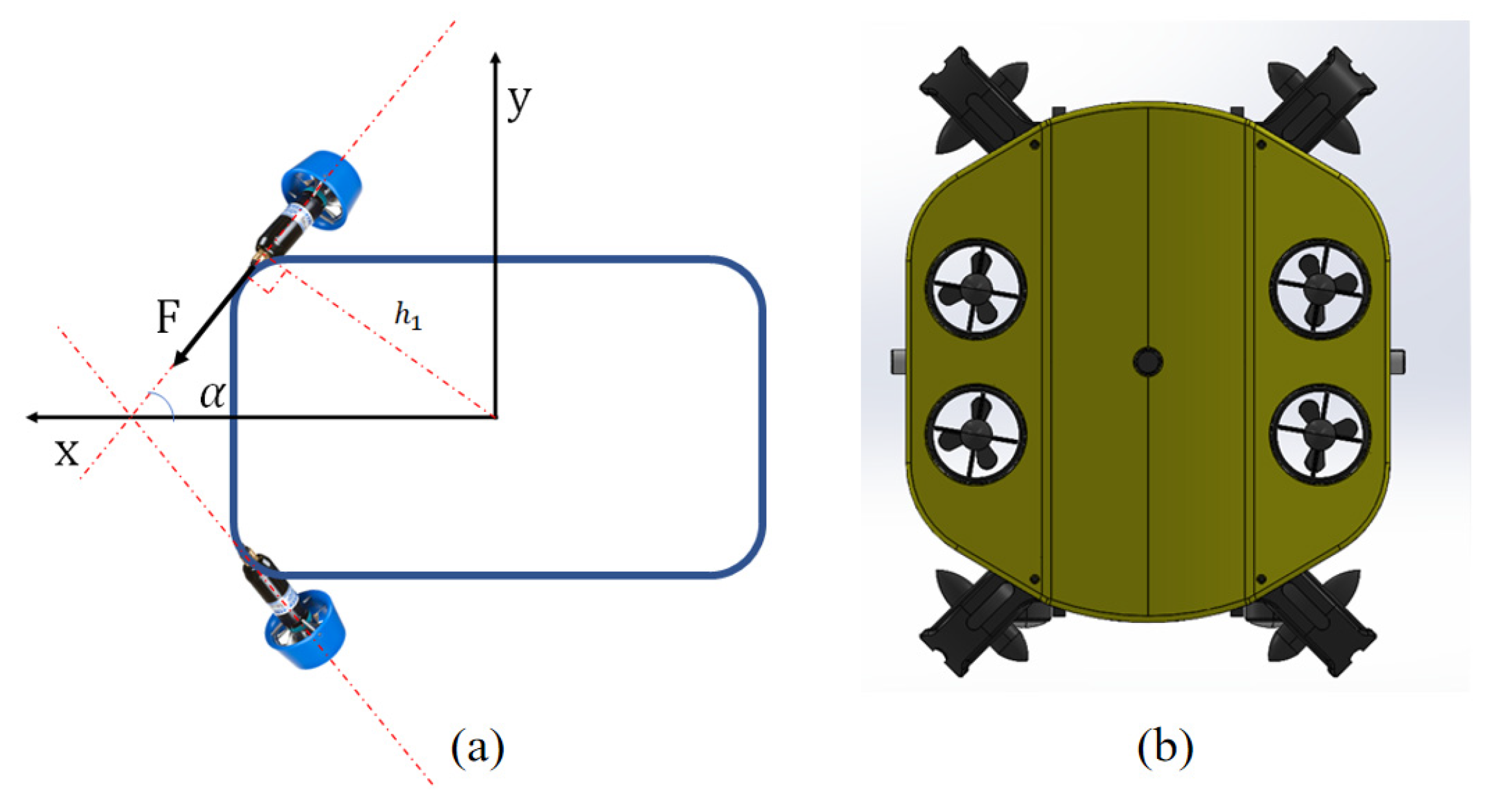
When designing the layout of the thrusters, the selection of the angle α is of critical importance. Firstly, the thrusters in the X-Y plane are related to three degrees of freedom of the underwater robot: surge, sway, and yaw. Secondly, the proportion of the robot’s travel distance or motion time in each of these three directions during a typical mission needs to be estimated. In addition, special consideration is given to the robot’s acceleration capability in these three degrees of freedom, as higher acceleration contributes to greater agility and responsiveness of the underwater robot. F is the propulsion force and h₁ is the arm of force. The angle α represents the angle between the force F and the X-axis, as shown in Figure 3. Based on these factors, the optimal value of α can be determined through an optimization approach. L and W are the absolute distances from the point of force application to the X and Y axes, respectively. Assume that the desired length proportions in the three directions are a: b: c, where a + b + c = 1. Based on geometric relationships, an analytical expression of a function with respect to α can be derived as follows:

$$f\left(\alpha \right)=aF\cos \left(\alpha \right)+bF\sin \left(\alpha \right)+cF{h}_1$$

(1)

$${\mathrm{h}}_1=L\sin \left(\alpha \right)+W\cos \left(\alpha \right)$$

(2)

The problem was modeled and converted into a standard optimization form:

$$\begin{gathered} \underset{\alpha }{\min } J=-f\left(\alpha \right) \\ \mathrm{s}.\mathrm{t}.\left\{\begin{array}{c}F\cos \left(\alpha \right)-m{\alpha }_x\ge 0\\ F\sin \left(\alpha \right)-m{\alpha }_y\ge 0\\ F{h}_1-I{\alpha }_z\ge 0\\ \alpha \ge 0\\ {\displaystyle \frac{\pi }{2}}-\alpha \ge 0\\ F-F_{\min }\ge 0\end{array}\right. \end{gathered}$$

(3)

Here, αₓ, αᵧ, and α_z represent the minimum linear accelerations in the X and Y directions and the minimum angular acceleration about the Z-axis, respectively. F_min is the minimum thrust required for the underwater robot to operate. I denotes the moment of inertia, and m is the mass of the AUV. The optimization problem is solved using the Sequential Quadratic Programming (SQP) algorithm. SQP is an iterative method that is particularly well suited for constrained optimization problems. It approximates the global optimum by successively solving quadratic sub-problems.

The constraint parameters in Equation (3) are designed as follows:

$$\begin{gathered} {\alpha }_x=0.5 \mathrm{m}/{\mathrm{s}}^2,{\alpha }_y=0.5 \mathrm{m}/{\mathrm{s}}^2,{\alpha }_z=0.5 \mathrm{m}/{\mathrm{s}}^2 \\ a\text{:}b:c=1:1:1, F_{min}=0.35 \mathrm{N},m=8kg \\ {h}_1=0.23311m, \mathrm{I}=0.179023258kg\cdot m^2 \end{gathered}$$

(4)

Since the thrust F generated by the thrusters does not affect the solution of the objective function, it is set to a constant value of 10. Solving the standard optimization problem described in Equation (3), the optimal solution is found to be $\alpha =\pi /4$.

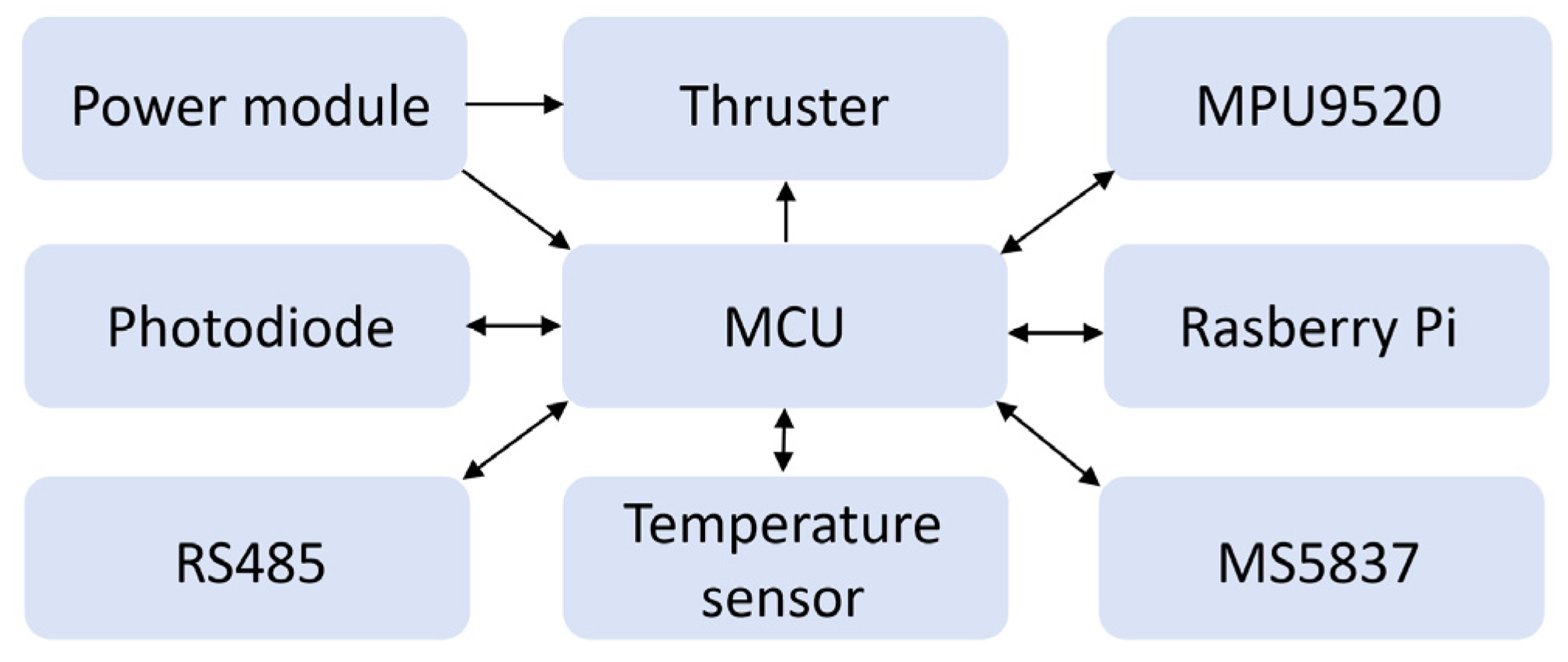
2.2. Hardware Design

The hardware of the underwater robot uses STM32F411 as the main control unit. An MPU9250 nine-axis gyroscope is employed to continuously acquire attitude data for controlling the robot’s orientation, while an MS5837 pressure sensor is used to obtain depth information, enabling precise control of the robot’s diving depth. The MCU must reserve I2C interfaces to communicate with both MPU9250 and MS5837. A Raspberry Pi is used for executing complex algorithms and computational tasks, communicating with the MCU via a TTL serial interface. The overall system structure is shown in Figure 4.

2.3. Software Design

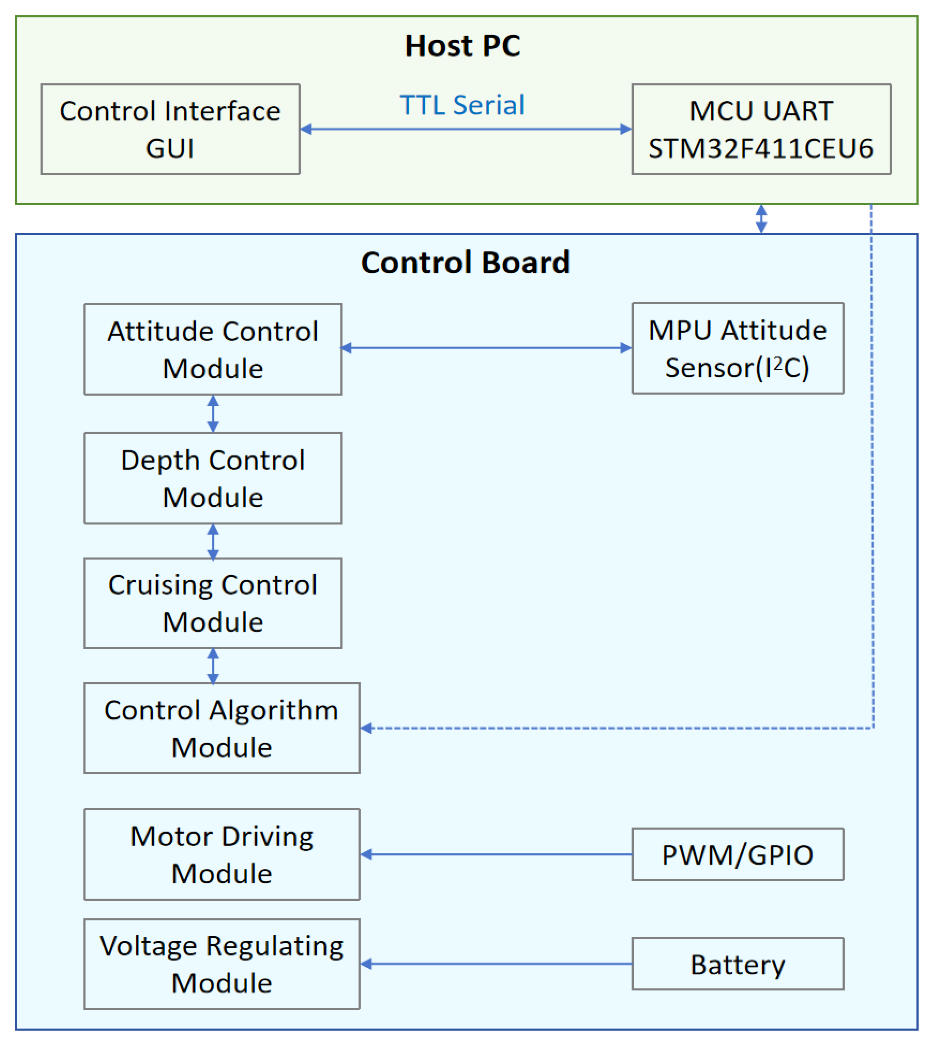
The overall software architecture, illustrated in Figure 5, plays a central role in the integrated design and agile motion control of the underwater robot. At the core of the system is a control board built around the STM32F411CEU6 microcontroller, which is interfaced with peripheral sensors, driver circuits, voltage regulation modules, and network communication ports. The software running on this embedded platform is responsible for acquiring real-time data on the robot’s attitude and depth and executing control algorithms to realize key functionalities such as self-stabilization, depth holding, and GPS-guided navigation. Through a TTL serial interface, the onboard software also enables seamless data exchange with the host computer, supporting higher-level mission planning and monitoring.

To ensure precise attitude estimation and rapid response to dynamic underwater conditions, the software integrates a high-performance inertial measurement unit (IMU), MPU9250, as the primary attitude sensor. MPU9250 delivers fused orientation data—including rotation matrices, quaternions, and Euler angles—via an I²C interface. The microcontroller communicates with the sensor through the SCL and SDA pins, enabling efficient data retrieval.

Internally, the MPU9250 uses seven ADC channels to convert physical motion parameters such as gravitational acceleration and angular velocity into electrical signals, storing them in internal registers. The software reads these registers to obtain real-time attitude information and configures the IMU’s operating modes by writing to its control registers. This tightly integrated hardware–software architecture enables the underwater robot to perform responsive, stable, and precise motion control in complex underwater environments.

3. Hydrodynamic Performance Analysis

Underwater robots are subjected to various forces during navigation, primarily including radiation forces, external forces from the marine environment, and thrust from actuators. Due to the complex structure of underwater robots, it is difficult to obtain accurate data models using traditional empirical formulas. Therefore, this paper employs numerical simulation methods to conduct hydrodynamic simulations of an underwater AUV.

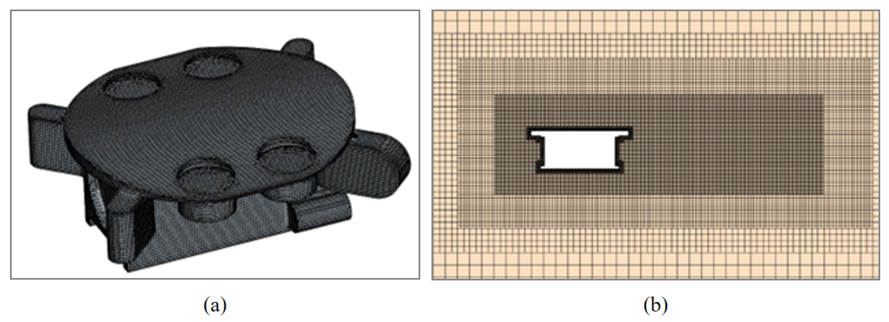
In this study, the software STAR-CCM+ was used to simulate and calculate the drag force. The SST k–ω turbulence model was selected for the simulation. A three-dimensional rectangular water body was chosen as the computational domain. The underwater vehicle was placed in an infinite seawater environment. The front face in the longitudinal direction was defined as a velocity inlet, where a prescribed inflow velocity was applied. The rear face was set as a pressure outlet, with the reference pressure taken as the standard atmospheric pressure, corresponding to a gauge pressure of zero. The surfaces of the underwater vehicle and the lateral boundaries of the domain were defined as no-slip walls.

The computational domain was meshed using a trimmed mesh approach, and a three-layer mesh transition zone was established to ensure the accuracy of the simulation results. The total number of mesh cells in the domain was 2,482,359. Figure 6a,b shows the surface mesh and the longitudinal section mesh of the computational domain, respectively.

The Grid Convergence Index (GCI) method was employed in this study to verify the mesh convergence. Three sets of grids with different resolutions—coarse, medium, and fine—were generated to calculate the longitudinal hydrodynamic resistance of the underwater vehicle. The mesh sizes are listed in

Table 3. Three sets of computational grids of different sizes.

No.	Mesh Quality	Minimum Mesh Size/m	Total Mesh Number
1	Fine	0.003	5,343,711
2	Medium	0.004	2,482,359
3	Coarse	0.005	1,382,596

. Φ₁, Φ₂, and Φ₃ represent the numerical results obtained from the coarse, medium, and fine grids, respectively. Φ_ext²¹ denotes the extrapolated value based on the medium- and fine-grid results. The relative error between the medium- and fine-grid results is denoted as e_α²¹, while the relative error between the fine-grid result and the extrapolated value is denoted as e_ext²¹. As the grid was continuously refined, the computational results exhibit a convergent trend, with a grid uncertainty less than 3.0%, as shown in

Table 4. Calculation results of grid convergence.

${\mathit{\varphi }}_1$	${\mathit{\varphi }}_2$	${\mathit{\varphi }}_3$	${\mathit{\varphi }}_{\mathit{e}\mathit{x}\mathit{t}}^{21}$	${\mathit{e}}_{\mathit{a}}^{21}$	${\mathit{e}}_{\mathit{e}\mathit{x}\mathit{t}}^{21}$	${\mathit{G}\mathit{C}\mathit{I}}_{21}$
37.85	38.25	38.31	37.72	0.011	0.003	0.42%

. Therefore, considering the factors of computation time and resource, the medium grid was adopted for subsequent calculations.

In the motion control equations, it was necessary to obtain the drag coefficients of the AUV. To determine the drag characteristics at different speeds, we selected three classic operating velocities—1, 2.5, and 3 knots—as test cases. The average simulation values after stabilization are presented in Table 1. The velocity distributions of the underwater robot at cruising speeds of 1 knot, 2.5 knots, and 3 knots are shown in Figure 7. A stagnation point was observed at the front, where the fluid velocity decreased. As the cruising speed increased, the low-velocity region at the rear became significantly larger, indicating an increase in wake length. For hydrodynamic drag reduction, we optimized the original rectangular hull into a streamlined, turtle-shell-shaped design with curved surfaces. Through hydrodynamic simulation analysis, we found that the turtle-shell-shaped outer casing reduced drag by 22% compared to a rectangular form, as shown in

Table 5. Comparison of resistance under different speeds.

Speed/Knot	Turtle Shell Shape Resistance/N	Rectangular Shape Resistance/N
1.0	6.40	7.80
2.5	38.25	45.90
3.0	54.61	66.62

. The derived drag coefficients were incorporated into the motion control model, enhancing real-time responsiveness. This work demonstrates a seamless integration of simulation and control, advancing the design of agile and efficient underwater robots.

4. Adaptive Event-Triggered Predictive Control Algorithm

The core idea of event-triggered control (ETC) is to update control inputs only when specific triggering conditions are met—such as when system state changes exceed a predefined threshold—rather than relying on continuous sampling and actuation. This study uniquely integrates ETC with the agile motion control of underwater robots, addressing key challenges in resource efficiency and performance under dynamic marine conditions. Unlike traditional periodic control, ETC significantly reduces communication bandwidth and energy consumption by transmitting data only when necessary. Moreover, it enhances responsiveness in complex underwater environments by enabling real-time, condition-based adjustments. To further explore its potential, this research implements both event-triggered PID control and nonlinear model predictive control (NMPC), offering a novel framework for improving underwater robot agility and robustness in uncertain conditions.

The primary motivation for employing an event-triggered approach lies in its efficiency in resource utilization and its capability to handle the computational constraints often encountered in embedded systems for underwater robotics.

In traditional time-triggered control, the controller updates its actions at fixed time intervals, regardless of whether the system state has significantly changed. While simple and predictable, this can lead to unnecessary computations and communications, especially in systems with limited bandwidth or power constraints, as is often the case in underwater environments. In contrast, an event-triggered control scheme updates the control input only when a predefined condition or “event” is satisfied. Compared with the state of the art, it helps to reduce computational load and energy consumption. It may increase complexity in triggering condition design and potential for Zeno behavior, which can be avoided by incorporating a minimum inter-event time.

4.1. Event-Triggered PID Algorithm

The cascade PID control algorithm is a feedback control strategy in which multiple control loops work in coordination. It is widely used in complex systems that require multi-level control. Compared to the traditional single PID control, cascade PID employs an inner loop and an outer loop to optimize different dynamic characteristics separately, enhancing both control accuracy and system stability. The outer PID loop is responsible for controlling slower-varying variables (such as position or attitude), while the inner PID loop handles faster dynamic changes (such as speed or acceleration). The advantage of cascade PID lies in its ability to decouple control tasks across different time scales, reduce delay and cumulative error, and improve both control precision and response speed.

The structural model of the control system based on the event-triggered cascade PID (ET-CPID) algorithm studied in this section is shown in Figure 8. In this system, a PID controller is used to adjust the AUV’s control inputs, ensuring that the system follows the desired trajectory or velocity according to the given target. Within this control system, the state variable x(t_i) and the reference value x_r interact with the PID controller through a feedback loop. The change in velocity is used as part of the control input, which directly influences the motion of the AUV. The system also incorporates an event-triggered mechanism, which monitors changes in the system state in real time based on predefined trigger conditions. This mechanism evaluates the feedback state variable information to determine whether the trigger condition is satisfied, thereby deciding whether to update the control output.

The key to event triggering lies in the design of the trigger condition. The condition adopted in this paper is shown in Equation (5).

$$\left|e\left(t_k\right)-e\left(t_s\right)\right|>e_{\lim }or {\mathrm{T}}_{act}\ge {\mathrm{T}}_{\max }$$

(5)

A new control signal is computed either when the absolute difference between the current error e(t_k) and the error at the last control update e(t_s) exceeds a predefined threshold e_lim or when the elapsed time, T_act, since the last sampling exceeds the maximum allowable interval, T_max. The latter condition serves as a simple safety mechanism, ensuring that under transient conditions (such as setpoint changes or load disturbances), the controller operates at the nominal sampling time, while under steady-state conditions, it operates at the maximum sampling interval.

4.2. Nonlinear Model Predictive Control

The desired trajectory of the underwater robot is defined as shown in Equation (6), X_ref is the six-degree-of-freedom reference state value of the underwater AUV.

$$X_{ref}={\left[x_{ref},y_{ref},z_{ref},{\phi }_{ref},{\theta }_{ref},{\psi }_{ref},v_{xref},v_{yref},v_{zref},{\omega }_{xref},{\omega }_{yref},{\omega }_{zref}\right]}^T$$

(6)

The objective of trajectory tracking control is to minimize the error between the actual state of the AUV and the desired state as much as possible. The discrete system model of the control objective is defined as ${\mathrm{x}}_{k+1}=f\left({\mathrm{x}}_k,u_k\right)$. The tracking error at the (k)-th discrete time step is defined as ${\mathrm{x}}_k^e={\mathrm{x}}_k{-\mathrm{x}}_k^r$, and the penalty function of the NMPC controller can thus be expressed as

$$\mathrm{J}\left({\mathrm{x}}_k^e,u\right)={\mathrm{x}}_k^{eT}{Q}_{end}{\mathrm{x}}_k^e+{\displaystyle \sum _{i=0}^{N-1}\left({{\mathrm{x}}_{k+1}^e}^{T}Q{\mathrm{x}}_{k+1}^e+u_{k+i}^{T}R{u}_{k+i}\right)}$$

(7)

Q is the state penalty matrix, Q_end is the terminal state penalty matrix, and R is the orthogonal identity matrix. By computing the full set of desired states at different time steps along the reference trajectory and inputting them into the NMPC controller as reference states, the control output at the current time step can be obtained, thereby enabling the tracking of the desired trajectory.

The proposed control strategy, based on an adaptive event-triggered mechanism, is illustrated in Figure 9. This strategy employs an independently designed event-triggering scheme that intelligently evaluates the system state to dynamically determine the communication schedule across the sensor–controller–actuator loop, significantly reducing redundant data transmission between components.

Compared to traditional periodic sampling or tightly coupled triggering schemes, the modular architecture of the proposed mechanism separates communication scheduling from control law design. This not only enhances system flexibility but also introduces an adaptive, dynamically tuned gain based on tracking error, which effectively compensates for the effects of uncertain disturbances, sampling quantization errors, and actuation delays.

The event-triggered error is typically defined as the deviation between the current system state, ${\mathrm{x}}_t$, and the desired state, ${\hat{x}}_t$, i.e.,

$$e\left(t\right)=\mathrm{x}\left(t+\Delta t\right)-\hat{x}\left(t\right)$$

(8)

where $\mathrm{x}\left(t+\Delta t\right)$ denotes the system state at the next time step, and ${\hat{x}}_t$ represents the value held in the zero-order hold at time (t). The corresponding event-triggering condition is given by:

$$‖e\left(t\right)‖\le e_T$$

(9)

where e_T is a predefined threshold. In this work, the computation error under the event-triggered mechanism is expressed as

$${\mathrm{e}}_T^2={\displaystyle \frac{\left(1-{\alpha }^2\right)}{L^2{‖r‖}^2}}\lambda \left(Q\right){‖\mathrm{x}\left(t\right)‖}^2+{\displaystyle \frac{1}{L^2}}{‖u_0^{*}‖}^2$$

(10)

where λ(Q) denotes the minimum eigenvalue of matrix Q, r is a lower triangular matrix with positive real diagonal entries satisfying R = rr^T, $\alpha \in \left(0,1\right)$ is a design parameter, and u₀^* represents the optimal control input obtained from the NMPC at each sampling instant. To adaptively regulate the event-triggering threshold, an adaptive dynamic gain is introduced:

$$\dot{L}=\max \left\{‖\mathrm{x}\left(t\right)-\mathrm{x}{\left(t\right)}_{ref}‖,0.01\right\}$$

(11)

where L denotes the adaptive dynamic gain, initialized at zero. Since its derivative is always positive, L is monotonically increasing and can grow sufficiently large. This gain adjusts its value based on the error between the current state and the reference state, thereby enabling a more effective regulation of the event-triggering threshold.

5. Simulation and Experimental Results

In this section, we first propose a unified evaluation coefficient to normalize different physical dimensions and quantitatively assess the motion performance of subsea autonomous underwater vehicles (AUVs). Using the subsea AUV designed in this study as a prototype, we then conducted both MATLAB R2022b simulations and controlled pool experiments. The performance of the motion control algorithm is evaluated through point-to-point trajectory tracking tasks, focusing on its accuracy, stability, and robustness under realistic operating conditions.

In this part of this study, we carried out a test to evaluate the AUV’s ability to move from an initial position (0, 0, 0) to a target (5 m, 10 m, 15 m) while maintaining fixed attitude angles (roll = 20°, pitch = 30°, yaw = 45°). The goal is to assess positioning accuracy and attitude stability under different control strategies (CPID, ET-CPID, AET-NMPC). The test parameters and results are shown in

Table 6. Experiment setup.

Item	Parameters
Reference Trajectory	(0, 0, 0) → (5 m, 10 m, 15 m)
Attitude Reference	Roll = 20°, Pitch = 30°, Yaw = 45°
Control Algorithms	CPID, ET-CPID, AET-NMPC
Performance Metric	RMSE (Position and Attitude)

.

5.1. Evaluation Index of Control Algorithm

In this study, the underwater robot exhibits six degrees of freedom (6-DOF) in its motion characteristics. When evaluating control algorithms, it is not sufficient to assess each degree of freedom in isolation. To facilitate a more objective and comprehensive evaluation of the relative performance of different algorithms, a composite performance index is introduced. This index simultaneously considers the motion states across all six degrees of freedom, enabling a more scientific comparison of various control strategies and providing a reliable basis for subsequent optimization and improvement.

$${\mathrm{X}}_{norm}={\displaystyle \frac{X}{X_{ref}}}$$

(12)

Given that the experimental data involve variables with different units and magnitudes, a normalization process is applied to ensure dimensionless data representation. This standardization ensures consistency across different motion axes during computation. Specifically, the state values are divided by their corresponding reference values to eliminate dimensional discrepancies, as shown in Equation (12):

$$\begin{array}{l}RMSE=\sqrt{{\displaystyle \frac{1}{M}}{\displaystyle \sum _{i=1}^M{\left|e_i\right|}^2}}\\ e_i=1-X_{norm}^i,i=1\dots M\end{array}$$

(13)

5.2. Simulation Results

In the design of NMPC, several key parameters need to be configured, including velocity constraints, position constraints, a state penalty matrix, and a control penalty matrix. In this study, a commonly used linear quadratic cost function is adopted, in which the state penalty matrix and the terminal state penalty matrix are set as follows:

$$\begin{array}{l}Q=diag(6,6,6,0.1,0.1,0.1)\\ Q_{end}=diag(30,30,30,1,1,1)\end{array}$$

(14)

The control penalty matrix is defined as

$$R=diag(1,1,1,1,1,1)$$

(15)

Both the prediction horizon and control horizon are set to 5. The constraints of the thrusters are defined as

$${\tau }_{\min }=-30N,{\tau }_{\max }=30N$$

(16)

The constraints applied in the NMPC design—on thruster output, velocity, position, and attitude angles—were chosen to reflect realistic the physical and operational limits of the AUV system. These constraints ensure that the control commands generated by the NMPC remain feasible and safe during execution. The constraints are aligned with those used in real-world tests.

The velocity constraints are set as

$$\begin{array}{c}-3.5\mathrm{m}/\mathrm{s}\le v_x\le 3.5\mathrm{m}/\mathrm{s}\\ -3.5\mathrm{m}/\mathrm{s}\le v_y\le 3.5\mathrm{m}/\mathrm{s}\\ -3.5\mathrm{m}/\mathrm{s}\le v_z\le 3.5\mathrm{m}/\mathrm{s}\\ -\pi /2\mathrm{rad}\le {\omega }_x\le \pi /2\mathrm{rad}\\ -\pi /2\mathrm{rad}\le {\omega }_y\le \pi /2\mathrm{rad}\\ -\pi /2\mathrm{rad}\le {\omega }_z\le \pi /2\mathrm{rad}\end{array}$$

(17)

The position and attitude angle constraints are set as

$$\begin{array}{c}-1000\mathrm{m}\le x\le 1000\mathrm{m}\\ -1000\mathrm{m}\le y\le 1000\mathrm{m}\\ 0\mathrm{m}\le z\le 2000\mathrm{m}\\ -\pi \mathrm{rad}\le \phi \le \pi \mathrm{rad}\\ -\pi \mathrm{rad}\le \theta \le \pi \mathrm{rad}\\ -\pi \mathrm{rad}\le \psi \le \pi \mathrm{rad}\end{array}$$

(18)

Among them, the yaw angle is constrained within the range of −π to π. Values beyond this range indicate the number of full rotations (in the positive or negative direction) the ROV has made relative to its initial orientation. Since the current NMPC prediction model cannot handle sudden transitions within the −π to π range, this method is used to address the issue.

Initially, the AUV is at rest, and its starting position is considered the origin. The initial values of its state variables are

$$q_0={\left[\begin{array}{cccccc}0& 0& 0& 0& 0& 0\end{array}\right]}^T,s_0={\left[\begin{array}{cccccc}0& 0& 0& 0& 0& 0\end{array}\right]}^T$$

(19)

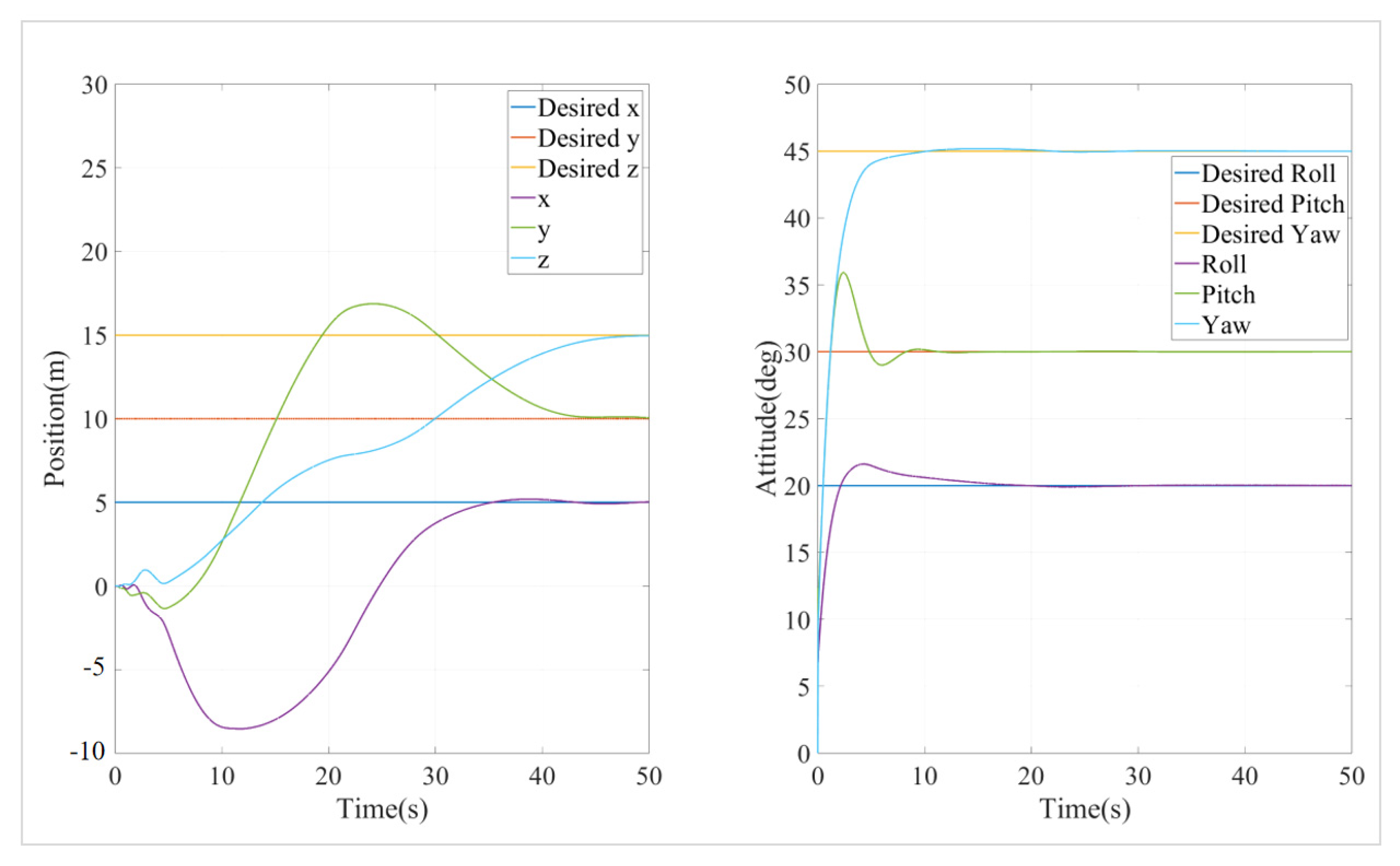
in which q₀ is the velocity initial state, and s₀ is the state initial state. Due to the highly complex terrain of the seabed, the underwater robot must be capable of maintaining a fixed attitude when navigating through challenging environments (e.g., passing through narrow openings). Therefore, the objective of this task was for the underwater robot to maintain a roll angle of 20 degrees, a pitch angle of 30 degrees, and a yaw angle of 45 degrees while moving from its initial position to the target position of (5, 10, 15). A simulation was conducted using the traditional cascaded PID control algorithm, and the PID parameters were tuned as much as possible within the simulation. The resulting position and attitude simulation outcomes are shown in Figure 10.

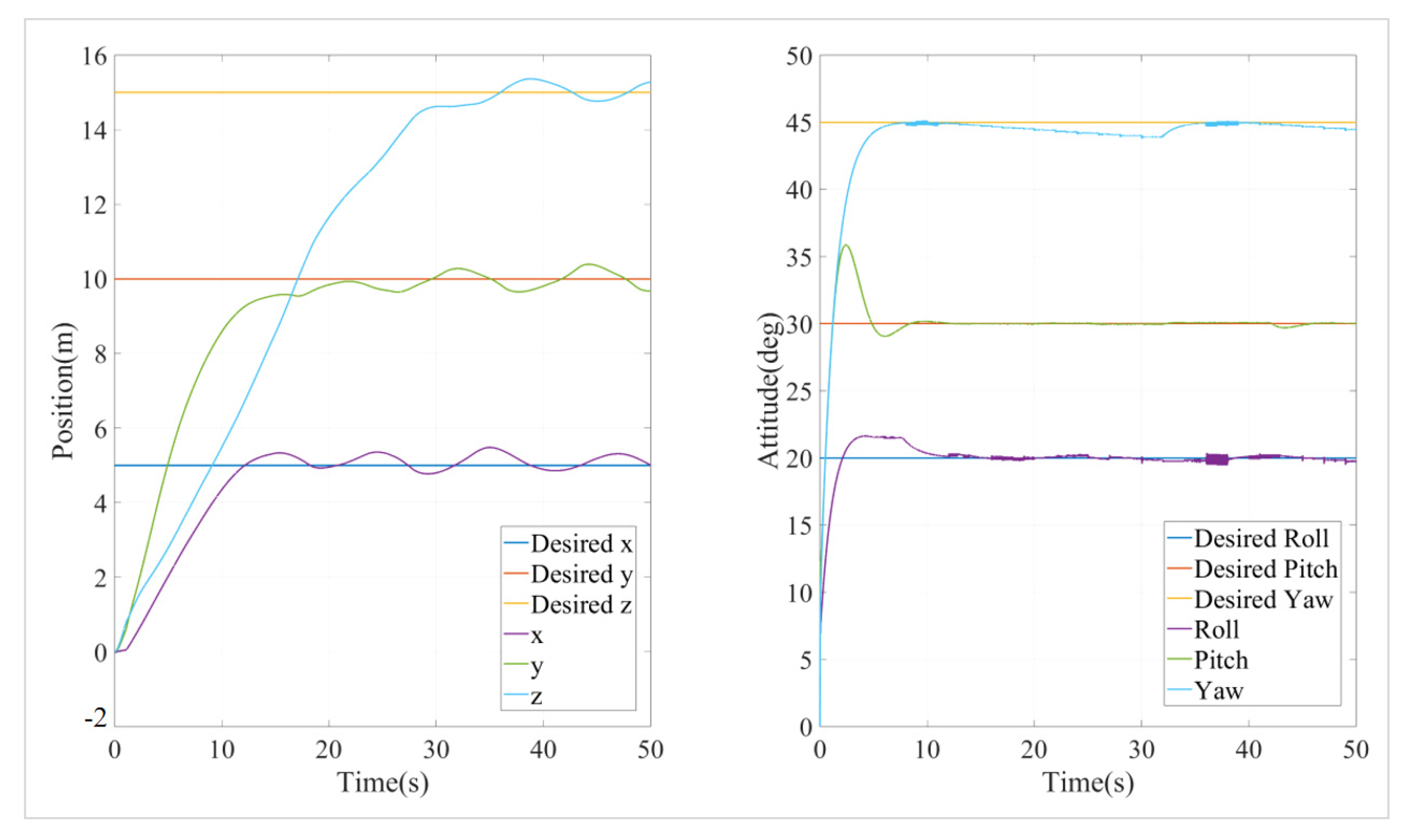
The simulation was conducted using an event-triggered cascade PID (ET-CPID) algorithm, with the trigger conditions set to e_lim = 0.1 and T_max = 10. The position and attitude simulation results are shown in Figure 10 and Figure 11.

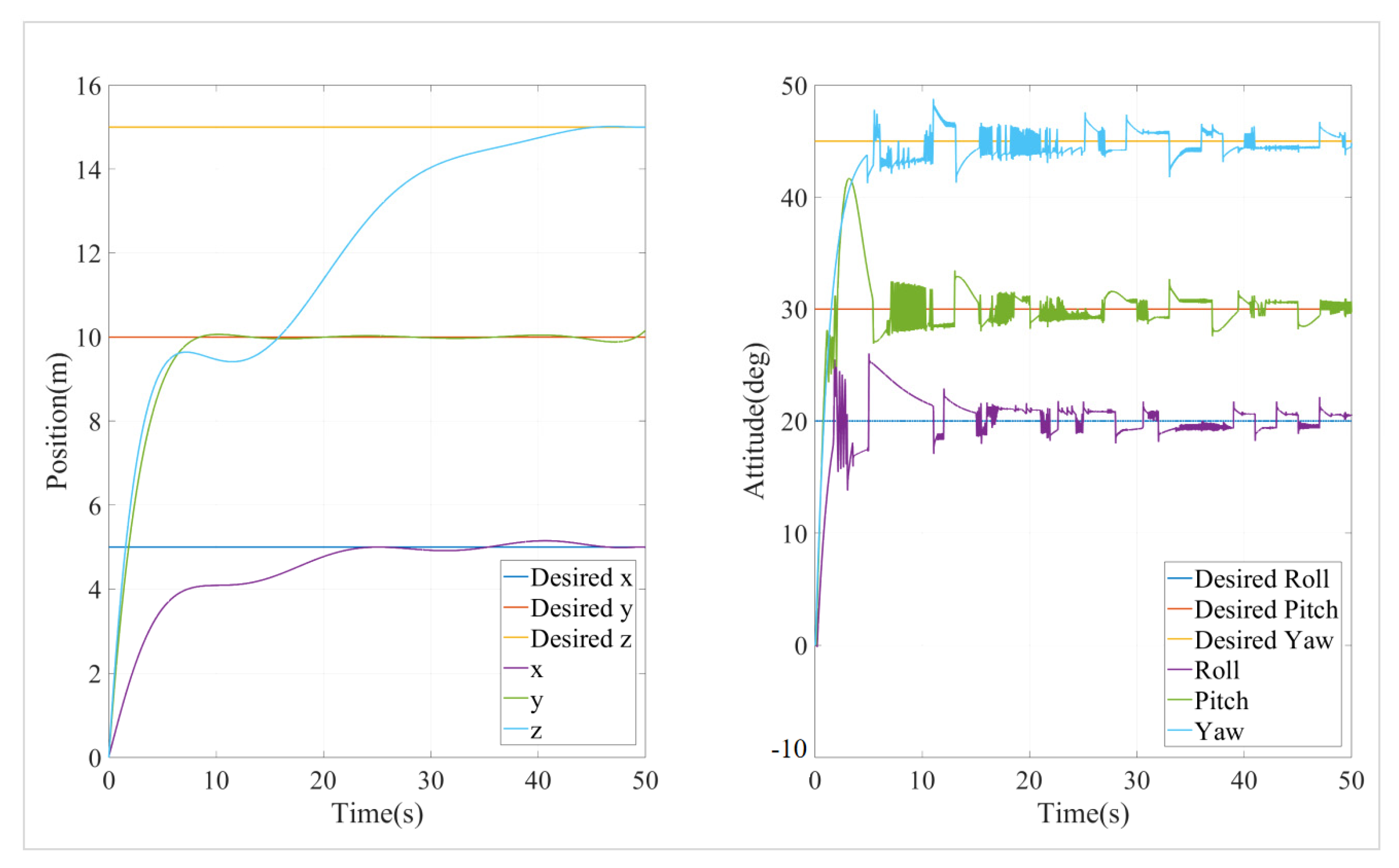
A simulation was also conducted using an adaptive event-triggered nonlinear model predictive control (AET-NMPC) algorithm, with the design parameter α set to 0.3. The position and attitude simulation results are shown in Figure 12, and the event trigger times and intervals between adjacent events are shown in Figure 13.

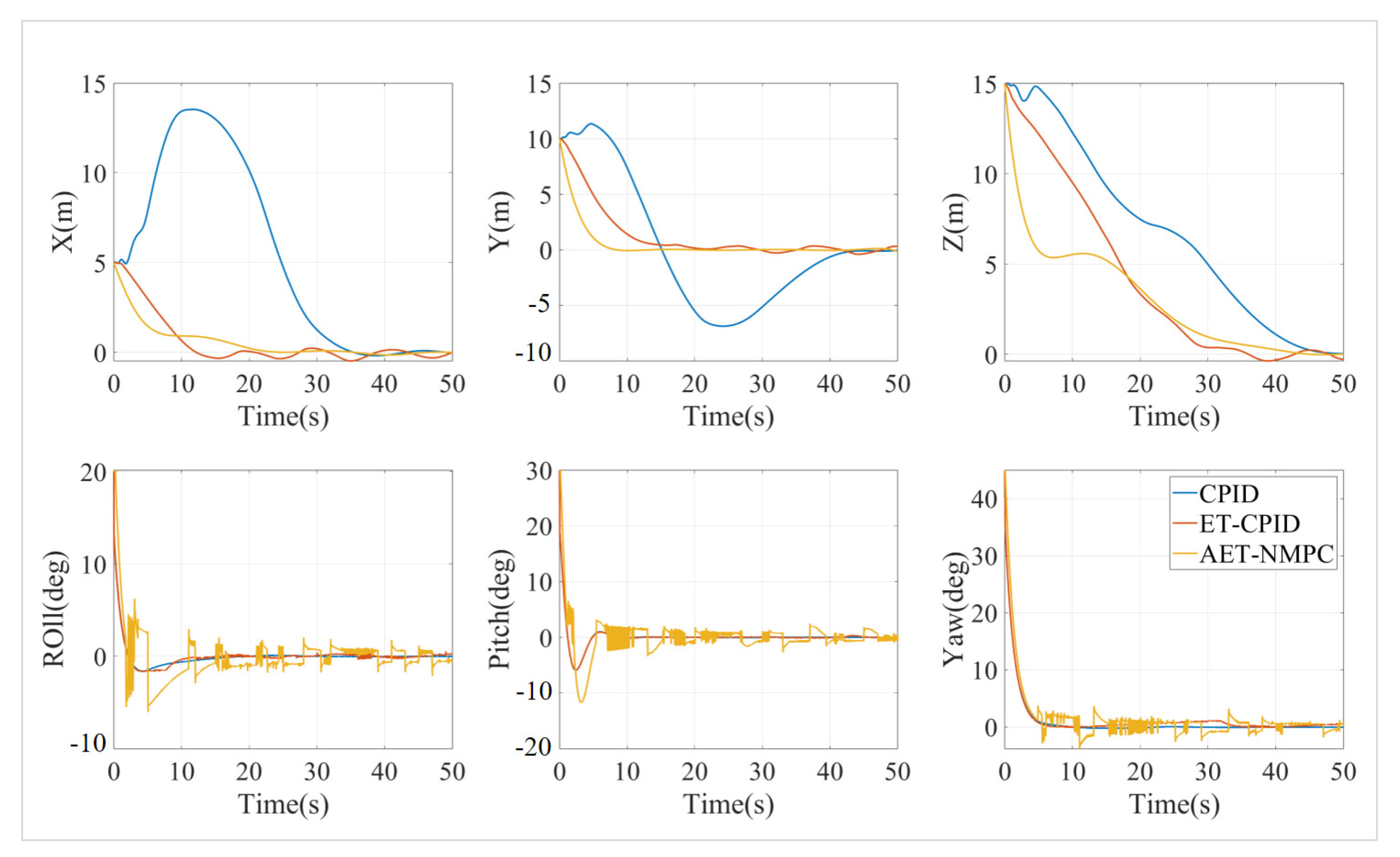
The trajectory plots of the three algorithms are shown in Figure 13, and the six-degree-of-freedom tracking errors are shown in Figure 14. It can be seen that all three algorithms successfully achieved point-to-point position tracking from the starting point to the endpoint, following a fixed desired attitude—namely, a desired roll angle of 20 degrees, a desired pitch angle of 30 degrees, and a desired yaw angle of 45 degrees—thus meeting the expected experimental objectives. Using the evaluation method described in Section 4.1, the simulation results were analyzed. Since the AUV’s state variables include both position (meters) and attitude angles (degrees), directly comparing their errors would be problematic due to the different units. To address this, the authors normalize the errors to make them dimensionless, ensuring a fair comparison. The formula is shown in (20)–(22).

$${\mathrm{X}}_{norm}={\displaystyle \frac{X}{X_{ref}}}$$

(20)

$${\mathrm{e}}_i=1-X_{norm}^i(i=1,\dots ,M)$$

(21)

$$RMSE=\sqrt{{\displaystyle \frac{1}{M}}{\displaystyle \sum _{\mathrm{i}=1}^M{\left|e_i\right|}^2}}$$

(22)

The dimensionless error values for each algorithm are shown in

Table 7. Non-dimensional error values of different algorithms.

Algorithm	CPID (%)	ET-CPID (%)	AET-NMPC (%)
	15.6966	5.7583	4.8928

.

In the point-to-point tracking task, the AET-NMPC algorithm performed the best, with a dimensionless error value of 4.89%. In comparison, the ET-CPID had an error of 5.76%, while the CPID showed an error of 15.70%. In terms of error, AET-NMPC outperformed ET-CPID by 0.87 percentage points and surpassed CPID by 10.81 percentage points. These results indicate that AET-NMPC offers superior path tracking accuracy in point-to-point tasks. AET-NMPC could accurately predict the future trajectory and dynamically adjust control parameters based on the error, significantly reducing deviations. Leveraging its model predictive capabilities, AET-NMPC responded more rapidly to path changes, achieving higher precision. Although ET-CPID’s error was slightly higher than that of AET-NMPC, it still demonstrated adequate performance in simple point-to-point tasks. However, it lacks the precise path adjustment capabilities of AET-NMPC. The CPID algorithm exhibited significantly larger errors, indicating that it is less effective at handling dynamic changes during control in point-to-point tasks, which leads to accumulating deviations.

5.3. Experimental Validation

The experiments were conducted in an indoor water tank equipped with glass observation windows, measuring 10 m in length, 6 m in width, and 4 m in depth. The experimental setup and conditions are illustrated in Figure 15.

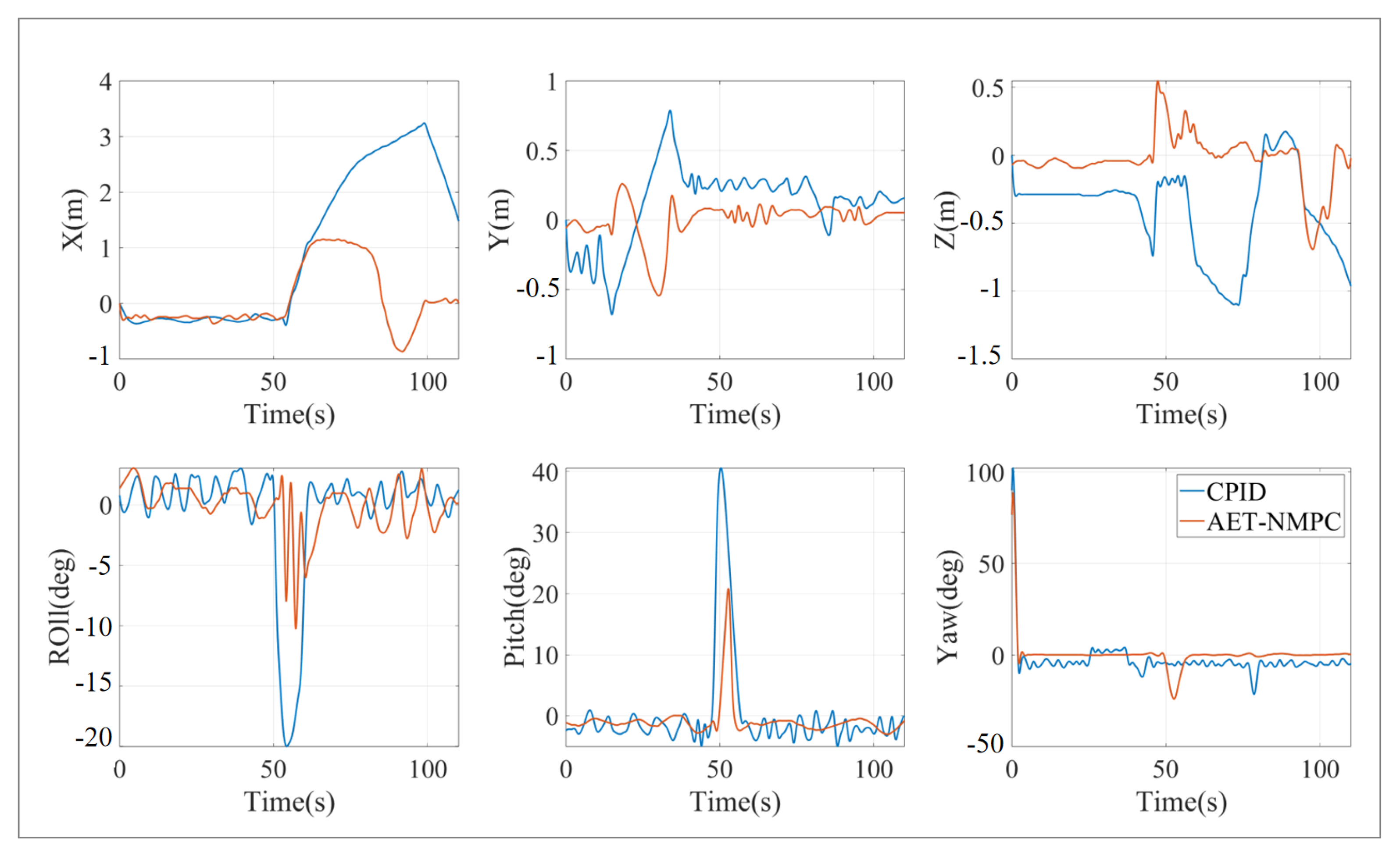
We conducted trajectory tracking experiments in the pool under the same conditions as the simulation, with the comparative results shown in Figure 16. Figure 16 presents the trajectory tracking points using both the adaptive event-triggered AET-NMPC algorithm and the event-triggered cascade PID algorithm. And the trajectory tracking error chart is shown in Figure 17. Experimental results reveal that the AET-NMPC algorithm, which is based on adaptive event-triggered mechanisms, offers higher accuracy and stability compared to the event-triggered cascade PID algorithm. The AET-NMPC approach demonstrates greater robustness in handling complex and dynamic environments. Although it imposes a higher computational load, the event-triggered mechanism effectively mitigates this by reducing the frequency of computations and communications, enhancing its practicality in real-world applications. Moreover, the predictive capability of the AET-NMPC algorithm allows for more precise adjustment of control inputs under external disturbances, significantly improving overall control accuracy.

In conclusion, the AET-NMPC algorithm with adaptive event-triggering outperforms the event-triggered cascade PID algorithm in complex environments, particularly in scenarios involving nonlinear dynamics and external disturbances. Despite its relatively higher computational demands, the AET-NMPC algorithm’s optimized control strategy delivers notable advantages in terms of accuracy and robustness, making it a promising solution for complex control tasks.

6. Conclusions

This paper presented the design and development of an autonomous underwater vehicle (AUV) aimed at navigating complex seafloor terrains with enhanced agility and trajectory tracking accuracy. To address this objective, a comprehensive approach was implemented, covering hydrodynamic optimization, mechanical structure design, and control algorithm development. Hydrodynamic simulations and shape optimization improved the vehicle’s stability and maneuverability, laying a solid foundation for precise motion control. A novel adaptive event-triggered model predictive control (AET-NMPC) algorithm was proposed to enhance control performance in dynamic and uncertain underwater environments. Through Simulink-based simulations and comparative analysis with conventional PID and event-triggered PID controllers, the AET-NMPC algorithm demonstrated significantly improved control accuracy and responsiveness. A small-scale AUV prototype was developed to validate the feasibility of the proposed system. Experimental results confirmed the effectiveness of the integrated hardware and software platform as well as the superior performance of the AET-NMPC algorithm, with the trajectory tracking error being reduced to 4.89%. Overall, this research successfully fulfilled its objective by achieving agile motion control and accurate trajectory tracking through the synergy of hydrodynamic optimization and advanced control strategies. These findings contribute to the advancement of AUV technologies, particularly for applications requiring high-precision navigation in complex underwater environments.

References

- Manley, J.E.; Marsh, A.G. Progress in autonomous underwater vehicles. Annu. Rev. Control. 2021, 52, 178–189. [Google Scholar]
- Ferreira, F.; Sousa, J.B.; Oliveira, R. AUV missions for oceanography: A review. Sensors 2020, 20, 5693. [Google Scholar]
- Mandal, S.; Tiwari, R.; Chakrabarty, A. A review on motion planning and control techniques for AUVs. Ocean. Eng. 2021, 235, 109380. [Google Scholar]
- Annamalai, A.R.; Wang, W. Autonomous underwater vehicles: A review on platforms, control and communication. Mar. Technol. Soc. J. 2022, 56, 42–56. [Google Scholar]
- Zhang, D.; Liang, Y.; Liu, J. Hydrodynamic modeling and experimental validation of an efficient AUV hull design. Ocean. Eng. 2021, 239, 109812. [Google Scholar]
- Kim, K.; Park, J. Design optimization of AUV considering maneuvering and hydrodynamic performance. Appl. Ocean. Res. 2020, 96, 102085. [Google Scholar]
- Ismail, A.R.; Karim, Z.A.; Mohamed, Z. Comparative performance analysis of torpedo-shaped AUVs. J. Mar. Sci. Eng. 2020, 8, 701. [Google Scholar]
- Chen, X.; Bose, N.; Brito, M.; Khan, F.; Millar, G.; Bulger, C.; Zou, T. Risk-based path planning for autonomous underwater vehicles in an oil spill environment. Ocean. Eng. 2022, 266, 113077. [Google Scholar] [CrossRef]
- Fossen, T.I.; Breivik, M. Nonlinear control of marine vehicles: Recent advances and future directions. Annu. Rev. Control. 2021, 52, 74–89. [Google Scholar]
- Cui, R.; Wang, H. Modeling and control of AUVs under ocean current disturbances. Ocean. Eng. 2020, 217, 107867. [Google Scholar]
- Wang, Z.; Liu, Y.; Jiang, H. Evaluation of PID and LQR control for underactuated AUVs. IEEE Access 2021, 9, 45367–45376. [Google Scholar]
- Li, Y.; Chen, C.L.P. Robust LQR–PID control of AUVs under modeling uncertainties. IEEE Trans. Syst. Man Cybern. Syst. 2020, 50, 2901–2911. [Google Scholar]
- Li, Y.; Wang, H. Adaptive sliding mode control of AUVs with input saturation. IEEE Trans. Ind. Electron. 2021, 68, 9750–9760. [Google Scholar]
- He, Y.; Zhang, W.; Liu, Y. Backstepping control for AUVs considering thruster dynamics and disturbances. Ocean. Eng. 2020, 198, 106963. [Google Scholar]
- Zhang, Y.; Yang, C. Nonlinear MPC for AUV trajectory tracking under constraints. Control. Eng. Pract. 2021, 109, 104731. [Google Scholar]
- Park, S.; Kim, M. Real-time model predictive control of AUVs with ocean current adaptation. Robot. Auton. Syst. 2022, 148, 103931. [Google Scholar]
- Wang, L.; Dunnigan, M.W. Thruster placement optimization for fault-tolerant AUV design. Ocean. Eng. 2021, 235, 109370. [Google Scholar]
- Tang, Y.; Cui, R. Optimal thruster configuration for over-actuated underwater robots. IEEE Trans. Ind. Inform. 2020, 16, 3276–3285. [Google Scholar]
- Cacace, J.; Finzi, A.; Lippiello, V. Fault-tolerant control in underwater vehicles using actuator reallocation. Robot. Auton. Syst. 2020, 124, 103361. [Google Scholar]
- Cui, R.; Liu, B.; Fu, M. Adaptive fault-tolerant control of AUVs using neural estimators. IEEE Trans. Ind. Electron. 2020, 67, 2170–2180. [Google Scholar]
- Li, Y.; Liu, J. Coordinated control for docking of AUVs under current disturbances. IEEE Trans. Control. Syst. Technol. 2021, 29, 2519–2530. [Google Scholar]
- Wang, X.; Zhang, Y. Disturbance-rejection control for AUVs using disturbance observer-based backstepping. Ocean. Eng. 2020, 217, 107919. [Google Scholar]
Figure 1.
Typical subsea AUV configurations.
Figure 2.
(a) Overall 3D model; (b) internal framework.
Figure 3.
(a)Thruster layout parameters; (b) top view of thruster layout.
Figure 4.
Hardware platform.
Figure 5.
Software architecture.
Figure 6.
(a) Mesh generation of underwater AUV; (b) mesh generation of calculation region.
Figure 7.
Speed distribution of underwater robot’s forward motion: (a) 1.0 knot, (b) 2.5 knots, and (c) 3.0 knots.
Figure 8.
Event-triggered PID algorithm control architecture.
Figure 9.
Event-triggered NMPC algorithm control architecture.
Figure 10.
Simulation results of position and attitude of cascade PID algorithm.
Figure 11.
Simulation results of position and attitude of event = triggered cascade PID algorithm.
Figure 12.
Simulation results of position and attitude of NMPC algorithm based on adaptive event triggering.
Figure 13.
Point-to-point trajectory diagram.
Figure 14.
Trajectory error diagram.
Figure 15.
Indoor experimental conditions.
Figure 16.
Trajectory tracking curves of different algorithms.
Figure 17.
Trajectory tracking error chart.