Energy-Optimized Path Planning and Tracking Control Method for AUV Based on SOC State Estimation

Abstract

Effective path planning in complex underwater environments serves as a critical determinant of autonomous underwater vehicle (AUVs) energy efficiency, while simultaneously influencing sensor operational demands and battery state-of-charge (SOC) dynamics. Systematic trajectory tracking emerges as a pivotal methodology for SOC optimization, enabling enhanced energy management through precision navigation control. This paper proposes a path planning and trajectory tracking control framework for autonomous underwater vehicles (AUVs) combined with battery state of charge (SOC) optimization. The framework incorporates the Grasshopper Optimization Algorithm (GOA) with the Artificial Potential Field Algorithm (APF) to achieve global path planning and local path optimization while minimizing energy consumption as an objective. Specifically, GOA is used for global path planning. APF further optimizes the path by introducing a SOC optimization strategy, in which high SOC consumption points are regarded as repulsive points and low SOC consumption points are regarded as attractive points. In addition, the trajectory tracking control adopts the model predictive control (MPC) method to ensure the accurate tracking of the planned path and dynamically manage the SOC states. Simulation results show that the proposed framework outperforms traditional methods in obstacle avoidance capability and SOC consumption, effectively improving energy efficiency and trajectory tracking accuracy.

1. Introduction

Autonomous underwater vehicles (AUVs), as an advanced underwater exploration and operation tool, have been widely used in marine science, resource exploration, and military applications in recent years [1]. The AUV’s practical autonomy and adaptable agility allow it to execute many duties in intricate underwater settings, such as marine surveying and mapping, ecological environment monitoring, and seabed geological exploration [2]. As technology advances, the usage of AUVs broadens, and their significance in scientific research and engineering is growing more evident [3]. However, the energy consumption of AUVs has always been one of the bottlenecks restricting their wide application due to the increase in size, weight, and sensor functions of AUVs when developing and designing AUVs [4], all of which limit the durability and driving range of the AUV to a certain extent. During the AUV mission, the battery’s state of charge (SOC) directly determines its sailing time and mission efficiency. Due to the difficulty of underwater energy replenishment, how to reasonably optimize the SOC in path planning and control and ensure the effective distribution of power on the path is one of the core issues to improve the endurance of AUV missions [5].

The majority of current AUV path planning techniques emphasize shortest path determination, obstacle evasion, or path optimization [6], and do not fully consider the impact of changes in battery SOC on energy consumption. This neglect leads to the fact that in actual tasks, AUVs may find it difficult to complete them due to the rapid drop in battery power during execution, so they cannot effectively extend the cruising time [7]. The path planning without SOC management not only affects the efficiency of task execution, but also may lead to task failure in complex environments, so integrating SOC optimization into path planning is the key to solving this problem [8].

Path planning algorithms aim to determine the most efficient path from an origin location to a destination. These algorithms can be broadly classified into three categories: traditional path planning methods, biologically inspired swarm intelligence methods, and machine learning methods [9,10]. Typically, traditional path planning algorithms rely on precise models of the problem or detailed information about the environment for their calculations. Commonly used traditional methods are the Dijkstra algorithm [11], Artificial Potential Field (APF) [12], A* algorithm, etc. [13]. Among them, the Dijkstra algorithm gradually determines the shortest path by traversing the global map and expanding the known shortest path set, but the discretization of the map will lead to a lack of smoothness in the planned path; the APF technique is a path planning algorithm that utilizes a virtual potential field, incorporating gravitational and repulsive forces to guide the intelligent agent in identifying the ideal route within the environment. Compared to the Dijkstra algorithm, the path determined by this method is more differentiable. Yet, it is susceptible to local optima, potentially resulting in the inability to identify the globally optimal path in intricate environments. In summary, these conventional approaches possess several significant shortcomings, including being time-consuming, having inadequate real-time performance, and a propensity to converge on local optima.

Due to the shortcomings of traditional methods, path planning is gradually developing towards artificial intelligence. Reference [14] introduces a multi-trajectory planning (MTP) problem for an autonomous underwater vehicle (AUV), considering the intricate underwater environment, the efficacy of each trajectory, and the variability among distinct trajectories, and formulates a comprehensive MTP model. By adopting a nesting strategy, attenuated alarm pheromones, and a diverse heuristic metric, an ant colony-based trajectory optimizer, MTrajPlanner, is developed to identify and maintain a set of high-quality solutions. Reference [15] amalgamates the genetic algorithm (GA), ant colony optimization (ACO) algorithm, and simulated annealing (SA) algorithm, enhancing GA through the introduction of novel energy consumption mutation operators, adaptive genetic operation probabilities, path self-smoothing, and trial crossover mechanisms, while also accounting for the impact of ocean currents. A novel heuristic algorithm fusion method is introduced to address the path-planning challenge for autonomous underwater vehicles (AUVs) in intricate underwater settings. Ref. [16] proposed a swarm intelligence optimization algorithm for locust optimization in 2017 and applied it to parameter optimization problems. GOA has a simple structure, few parameters, and strong stability. It is very competitive in terms of optimization accuracy and solution speed [17]; the algorithm’s unique adaptive mechanism effectively balances the global and local search processes [18].

In actual missions, AUVs not only need to plan a reasonable path but also need to track the path accurately [19]. However, the path tracking process will also be affected by external factors such as ocean current interference, causing the trajectory to deviate from the planned path and increasing additional energy consumption [20]. Existing path-tracking control methods mostly take stability and trajectory accuracy as the main goals without considering the real-time optimization of SOC and ignore the impact of energy consumption on trajectory adjustment. This control strategy, lacking SOC management, may cause the AUV to consume excessive battery power during path tracking, thereby shortening the vehicle’s endurance and affecting its stability and durability in complex missions.

Numerous control methodologies have attained elevated tracking precision, including sliding mode control [21], neural network control [22], and fuzzy control [23]. Furthermore, several published articles have enhanced the energy optimization of AUVs through the refinement of control methodologies. Reference [24] proposed an energy optimization control method based on economic model predictive control (EMPC) by considering the dynamic characteristics of AUV and the influence of ocean circulation. The EMPC controller optimizes two objective functions: one is the control energy consumption in the prediction time domain, and the other is the remaining energy consumption from the end of the prediction time domain to the target waypoint (energy-to-reach). Reference [25] proposed a new position error-constrained line tracking (PECLOS) control strategy based on the controller design of feedback linearization and the position error constraint mechanism. Reference [26] proposed an underwater communication system that combines time-division synchronous OFDM (TDS-OFDM) and non-orthogonal multiple access (NOMA), and uses energy recovery techniques to improve the energy efficiency of the system. Reference [27] proposed a hybrid energy-efficient routing protocol (HEERP) to optimize the energy consumption and data transmission efficiency of underwater wireless sensor networks (UWSNs) by combining DFS and BFS strategies. Experimental results show that HEERP outperforms conventional routing protocols in terms of energy consumption, network throughput and transmission delay.

Thanks to its benefits of rolling optimization and the explicit management of constraints, Model Predictive Control (MPC) has established itself as a well-developed technology in modern industry, as noted in [28]. Numerous scholars have explored the application of MPC in controlling Autonomous Underwater Vehicles (AUVs) [29]. The literature [30] presented an innovative hybrid agent-based MPC control method regarding resource efficiency. This method’s cost function takes into account fuel expenses, exergy loss costs, and primary exergy loss costs to minimize energy usage in maintaining indoor air temperature. In [31], a novel energy consumption cost function was introduced that incorporates controlled heating and cooling power parameters, demonstrating its efficiency through various test scenarios. However, there is a dearth of literature on the topic of optimizing AUV battery management systems utilizing Model Predictive Control (MPC) techniques. The design of the MPC control law hinges on the minimization of this cost function, which encompasses elements aimed at achieving specific control targets. Generally, this involves minimizing the discrepancy between the projected outcome and the original trajectory, along with the expected fluctuations in the input vector [32]. The Model Predictive Control (MPC) methodology has been prominent in the regulation of Autonomous Underwater Vehicles (AUVs) and Remotely Operated Vehicles (ROVs) due to its advantageous rolling horizon technique and its proficiency in constraint management. Simulations detailed in [33] demonstrated the practicality of MPC. Trials utilizing MPC controllers for AUVs and ROVs have yielded compelling results, showcasing MPC’s ability to maintain impressive control precision [34]. Nonetheless, the optimization of State of Charge (SOC) is not currently incorporated into the cost function of MPC.

This paper proposes a unified SOC optimization architecture based on AUV. In the path planning stage, a new GOA-PF method is proposed, in which the locust algorithm is used for global path planning, and the artificial potential field algorithm is used for local SOC optimization. The SOC reference is introduced, and the path points with large SOC changes are regarded as repulsive points, and the path points with small changes are regarded as attractive points so as to effectively allocate the energy consumption on the path. Secondly, the trajectory tracking control adopts the model predictive control (MPC) method to ensure the accurate tracking of the planned path and dynamically manage the SOC states.

This paper’s primary contributions are as follows:

• In view of the fact that AUVs cannot replenish energy underwater, a new GOA-PF path planning method for optimizing SOC is proposed.
• In view of the anti-interference ability of AUV path tracking and avoiding excessive energy loss, a SOC-optimized NMPC control method is proposed.
• An integrated framework of path planning and tracking control based on SOC optimization is proposed. By combining path planning with SOC optimization and continuing to pay attention to the dynamic management of SOC in the path tracking stage, the unified optimization of path selection and energy management during the AUV mission execution is achieved.

The remainder of this article is structured as follows:

Section 2 presents the mathematical model of the AUV, the three-dimensional environmental model, energy consumption, and the battery model. Section 3 delineates the comprehensive design process of the GOA-PF path planning algorithm. Section 4 presents the comprehensive design block diagram of the system and elaborates on the MPC controller design with a focus on SOC optimization. The simulation outcomes and conclusions are presented in Section 5 and Section 6, respectively.

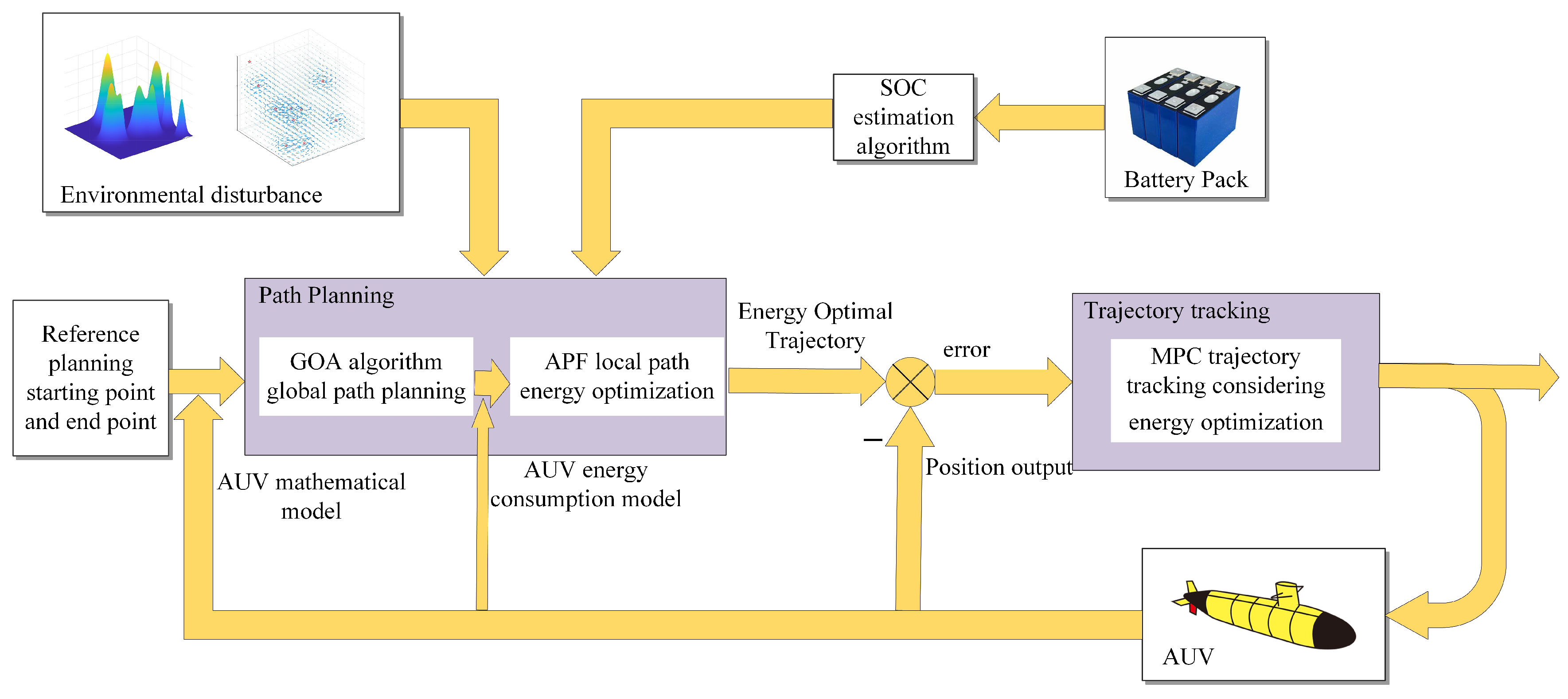
2. AUV System Description and Modeling

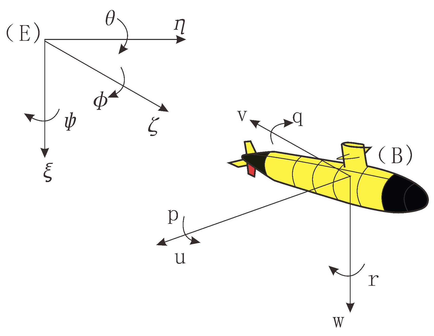
2.1. Kinematic and Dynamic Models

The Society of Naval Architects and Ocean Engineers (SNAME) [35] recommends that the origin of the inertial coordinate system I be positioned at the ocean surface’s beginning point, with the $E\zeta$ axis aligned with the reference heading. The stationary coordinate system B is affixed to the AUV, with its origin located at the center of gravity of the AUV and its principal axis aligned with that of the AUV. Figure 1 illustrates the corresponding system of coordinates.

The rotation matrix of the 6-DOF underwater robot is composed of three-axis basic rotation matrices. In geometric analysis, the basic rotation matrices of the X-axis, Y-axis, and Z-axis are as follows:

$$R_x\left(\varphi \right)=\left[\begin{array}{ccc}1& 0& 0\\ 0& cos\left(\varphi \right)& -sin\left(\varphi \right)\\ 0& sin\left(\varphi \right)& cos\left(\varphi \right)\end{array}\right]$$

(1)

$$R_y\left(\theta \right)=\left[\begin{array}{ccc}cos\left(\theta \right)& 0& sin\left(\theta \right)\\ 0& 1& 0\\ -sin\left(\theta \right)& 0& cos\left(\theta \right)\end{array}\right]$$

(2)

$$R_z\left(\psi \right)=\left[\begin{array}{ccc}cos\left(\psi \right)& -sin\left(\psi \right)& 0\\ sin\left(\psi \right)& cos\left(\psi \right)& 0\\ 0& 0& 1\end{array}\right]$$

(3)

Combining these basic rotation matrices, the rotation matrix R is as follows:

$$R=R_z\left(\psi \right)R_y\left(\theta \right)R_x\left(\varphi \right)$$

(4)

The relationship between direction and angular velocity is as follows:

$$J=\left[\begin{array}{ccc}1& sin\left(\varphi \right)tan\left(\theta \right)& cos\left(\varphi \right)tan\left(\theta \right)\\ 0& cos\left(\varphi \right)& -sin\left(\varphi \right)\\ 0& sin\left(\varphi \right)/cos\left(\theta \right)& cos\left(\varphi \right)/cos\left(\theta \right)\end{array}\right]$$

(5)

Therefore, the kinematics of the AUV in 6-DOF is

$$\dot{\eta }=\left[\begin{array}{cc}R& 0_{3\times 3}\\ 0_{3\times 3}& J\end{array}\right]\nu$$

(6)

Keep in mind that the following matrices stand in for the position vector and the generalized velocity vector, respectively:

$$\eta ={\left[\begin{array}{c}X,Y,Z,\varphi ,\theta ,\psi \end{array}\right]}^T$$

(7)

Referring [35] to the maneuvering model, the nonlinear equations of motion for the AUV kinetics have the following general form:

$$M\left(\dot{\nu }\right)+C\left(\nu \right)\nu +D\nu +g\left(\eta \right)=\tau$$

(8)

where M stands for the inertia matrix, C for the centripetal and Coriolis terms, and D for the hydrodynamic damping matrix in this context. To control the AUV’s motion, the control input variable $\tau =Bf$ is converted into force and torque via the matrix B, while the vector g represents the combined effects of buoyant and gravitational forces. Here is how the control input variable f is defined:

$$f={\left[\begin{array}{c}{T}_u,T_q,T_r\end{array}\right]}^T$$

(9)

where $T_u$ symbolize the thrust generated by propeller rotation, $T_q$ represent the vertical motion control force exerted by the left and right rudders, and $T_r$ signify the horizontal motion control force produced by the up and down rudders.

Assuming the AUV’s center of gravity ($x_g,y_g,z_g$) and buoyancy remain in one place, its six-DOF translational and rotational motion will be the following:

$$\begin{array}{cc}\hfill & m[\dot{u}-\nu r+wq-x_g(q^2+r^2)+y_g(pq-\dot{r})+z_g(pr+\dot{q})]=X_{total}\hfill \\ \hfill & m[\dot{v}-wp+ur-y_g(r^2+p^2)+z_g(qr+\dot{p})+x_g(qp+\dot{r})]=Y_{total}\hfill \\ \hfill & m[\dot{w}-uq+vp-z_g(p^2+q^2)+x_g(rq-\dot{q})+y_g(rp+\dot{p})]=Z_{total}\hfill \\ \hfill & I_x\dot{p}+(I_z-I_y)qr-(\dot{r}+pq)I_{xz}+(r^2-q^2)I_{yz}+(pr-\dot{q})I_{xy}\hfill \\ \hfill & +m[y_g(\dot{w}-uq+vp)-z_g(\dot{v}-wp+ur)]=K_{total}\hfill \\ \hfill & I_y\dot{q}+(I_x-I_z)rp-(\dot{p}+qr)I_{xy}+(p^2-r^2)I_{zx}+(qp-\dot{r})I_{yz}\hfill \\ \hfill & +m[z_g(\dot{u}-vr+wq)-x_g(\dot{v}-uq+vp)]=M_{total}\hfill \\ \hfill & I_z\dot{r}+(I_y-I_x)pq-(\dot{q}+rp)I_{yz}+(q^2-p^2)I_{xy}+(rp-\dot{p})I_{zx}\hfill \\ \hfill & +m[x_g(\dot{\nu }-wp+ur)-y_g(\dot{u}-wr+wq)]=N_{total},\hfill \end{array}$$

(10)

where m represents the vehicle’s mass, I denotes the moment of inertia in a particular axial or lateral direction, and ($X_{total},Y_{total},Z_{total}$) and ($K_{total},M_{total},N_{total}$) signify the total external forces corresponding to each degree of freedom.

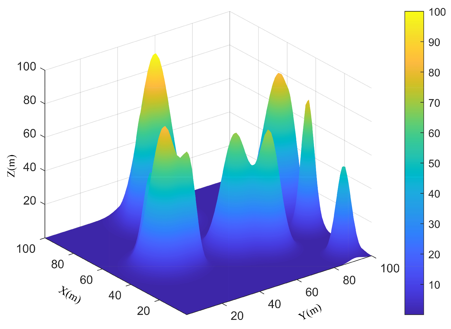
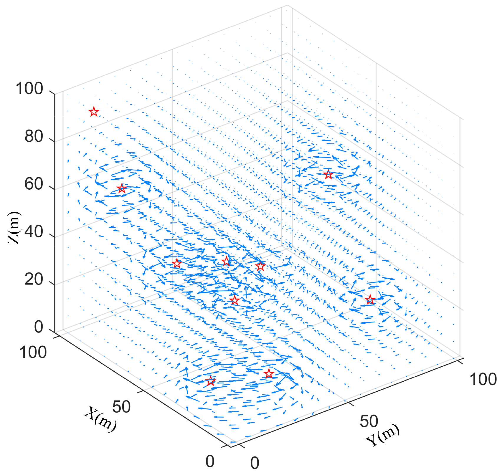
2.2. Underwater Environment Model

Complex physical elements in the underwater environment, including ocean currents, eddies, and impediments, significantly influence the course planning and trajectory tracking of autonomous underwater vehicles. The underwater environment model is used to simulate the actual operating environment of AUVs under different water currents and obstacle distributions so that the path planning process can take into account the interference caused by environmental factors such as ocean currents.

In the context of elevated natural mountains within the navigation environment, an exponential function is employed for their characterization, and the theoretical framework can be articulated as follows:

$$z\left(x,y\right)=\sum _{i=1}^n{h}_{i}exp[-{\left({\displaystyle \frac{x-x_i}{x_{si}}}\right)}^2-{\left({\displaystyle \frac{y-y_i}{y_{si}}}\right)}^2]$$

(11)

where, x and y denote the horizontal and vertical positional components of the seafloor topography, respectively; ($x_i$, $y_i$) indicates the central coordinates of the ith peak; n signifies the total number of peaks; $h_i$ is the terrain parameter that affects the height; $x_{si}$ and $y_{si}$ are the attenuation and control slopes of the ith peak along the x-axis and y-axis, respectively. Figure 2 shows the seafloor topography, which represents the real environment of the seafloor by establishing seafloor topographic constraints.

By analyzing the movement of ocean currents in reality, multiple single-point Lamb vortices are superimposed to simulate the movement state of real ocean currents. The mathematical expression formula is as follows:

$$\begin{array}{cc}\hfill V_x\left(r\right)& =-\lambda \times {\displaystyle \frac{y-y_0}{2\pi (r-r_0)}}\times \left(1-e^{-{\left({\displaystyle \frac{r-r_0}{\zeta }}\right)}^2}\right)\hfill \\ \hfill V_y\left(r\right)& =\lambda \times {\displaystyle \frac{x-x_0}{2\pi (r-r_0)}}\times \left(1-e^{-{\left({\displaystyle \frac{r-r_0}{\zeta }}\right)}^2}\right)\hfill \\ \hfill V_z\left(r\right)& ={\displaystyle \frac{\lambda }{\pi {\zeta }^2}}\times e^{-{\left({\displaystyle \frac{r-r_0}{\zeta }}\right)}^2}\hfill \end{array}$$

(12)

where r is the position state variable, x and y represent the horizontal and vertical position components of the ocean current, $V_i\left(r\right)$ are the velocity components of the ocean current in the horizontal, vertical, and vertical directions, $x_0$, and $y_0$ are the horizontal and vertical position constants of the ocean current, respectively, and $\lambda$, $\zeta$, and $r_0$ are the coordinates of the eddy intensity, eddy radius, and eddy center position, respectively. Figure 3 shows the generated random eddy field, with the red pentagram as the eddy centre and the blue symbols as the random eddy field. If $\lambda$ is greater than 0, the eddy is counterclockwise; if $\lambda$ is less than 0, the eddy is clockwise.

2.3. Energy Consumption Model

The energy consumption of AUVs in underwater missions directly affects their endurance and the effectiveness of mission execution. Establishing an energy consumption model can quantify the power consumption of AUVs at different speeds and attitude adjustments and help evaluate the impact of path selection and control strategies on energy utilization. During the execution of tasks by the AUV, the main energy consumption comes from the computing energy consumption of control system equipment, the energy consumption of AUV navigation resistance, and the energy consumption of actuators.

The energy consumption of navigation resistance generally includes the change in navigation resistance caused by the change in AUV longitudinal inclination angle and the resistance caused by the change in the rudder angle [4]. For the cross-shaped rudder of an underwater vehicle, the rotation of each rudder will generate forces and moments in all directions of the AUV. The lift Li and longitudinal resistance XR of the rudder can be expressed by Equations (13) and (14):

$$L_i={\displaystyle \frac{1}{2}}{C}_{Li}(\lambda ,{\delta }_i)u^2\rho A$$

(13)

$$X_R=\sum _{i=1}^4{\displaystyle \frac{1}{2}}{C}_D(\lambda ,{\delta }_i)\rho A{u}^2$$

(14)

where u is the longitudinal speed of the AUV, i is the number of the rudder, A is the rudder area, and the lift coefficient $C_{Li}$ and the drag coefficient $C_D$ are obtained by interpolating the rudder angle of the i rudder, and $\rho$ is the seawater density.

The control quantity of the AUV steering system is the rudder angle, so the energy consumption modeling analysis is carried out based on the rudder angle. The energy consumption of the motor driving the rudder surface is shown in Formula (15):

$$P_{\delta }={\displaystyle \frac{W}{\eta }}={\displaystyle \frac{M_{\delta }\times \dot{\delta }}{\eta }}$$

(15)

where $P_{\delta }$ denotes the power consumption of the servo system, W denotes the output power of the servo system, $\eta$ indicates the operational efficiency of the servo system, $M_{\delta }$ signifies the total load torque of the rudder surface, and $\delta$ refers to the angular velocity of the rudder. The overall load torque on the rudder surface comprises the torque $M_l$ generated by the hydrodynamic force and the system’s friction torque, expressed as follows:

$$M_{\delta }=M_l+M_f$$

(16)

where $M_l$ is linearly positively related to the product of the square of the AUV’s forward velocity $u_0$ and the steering angle $\delta$, which can be expressed as follows:

$$M_l=\mathit{\epsilon }{\mathit{u}}_0^2\delta$$

(17)

where $\epsilon$ is the torque coefficient, which is 0.0274 through relevant calculation. Compared with the hydrodynamic torque $M_l$, the friction torque $M_f$ is very small and can be approximated as tiny, so it can be ignored. The work required for the rudder angle to change from the initial rudder angle ${\delta }_0$ to $\delta$ is as follows:

$$W_r={\int }_0^{\left|{\displaystyle \frac{\delta -{\delta }_0}{\delta }}\right|}{M}_{\delta }{u_0}^2\delta \left(t\right)\dot{\delta }dt$$

(18)

For the modeling of propeller thrusters, we need to express the propeller thrust $T_p$ and torque $Q_p$ according to the following equations:

$$T_p=\rho ·D^4·K_T\left(J_0\right)·n·\left|n\right|$$

(19)

$$Q_p=\rho ·D^5·K_Q\left(J_0\right)·n·\left|n\right|$$

(20)

where D is the propeller diameter, $K_T$ and $K_Q$ are dimensionless thrust and torque coefficients, n is the propeller speed, and we consider $K_T$ and $K_Q$ as polynomial forms as follows:

$$\begin{array}{c}\hfill K_T=k_{t1}·J_0^2+k_{t2}·J_0+k_{t3}\\ \hfill K_Q=k_{q1}·J_0^2+k_{q2}·J_0+k_{q3}\end{array}$$

(21)

where $J_0={\displaystyle \frac{u}{n\times D}}$ is the advance coefficient, $k_{t1}$ to $k_{t3}$ and $k_{q1}$ to $k_{q3}$ are the coefficients suitable for propeller design, and the propeller parameters are listed in the table.

The effective thrust $T_p$ of the propeller is the longitudinal resistance overcome by the AUV during navigation, so the propeller energy consumption is

$$P_{Thrust}={\alpha }_P{\left(T_P\right)}^2$$

(22)

where ${\alpha }_p={\displaystyle \frac{1}{D}}\sqrt{{\displaystyle \frac{1}{2\pi \rho }}}$ is the propeller power coefficient.

In summary, the total energy consumption of an autonomous underwater vehicle throughout the movement is indicated in Formula (23):

$$J_P=W_{RS}+W_P+W_r+W_{cs}$$

(23)

where $W_{RS}={\int }_{t_0}^t(F_D+X_R)udt$, $W_P={\int }_{t_0}^t{P}_{thrust}dt$, $W_r$ represents the energy consumption of resistance, propeller and steering gear in a certain action time domain, and $W_{cs}$ represents the power resource consumption of the control system.

2.4. Battery Model

A 32-cell lithium iron phosphate battery pack with a nominal energy capacity of 3 kWh is used as the energy storage unit of the AUV power system. This study omits the influence of temperature on the battery [8] and employs a rudimentary internal resistance model to delineate the dynamic characteristics of the battery, wherein $V_{oc-bat}$ denotes the open circuit voltage, $R_{bat}$ signifies the total internal resistance of the battery pack, $V_{bat}$ indicates the battery output voltage, and $I_{bat}$ represents the battery current. The correlation among $I_{bat}$, $P_{bat}$ (denoting battery output power), $E_{bat}$ (indicating remaining battery energy), $V_{bat}$, and SOC (representing the state of charge of the battery) can be articulated as follows:

$$P_{bat}=V_{bat}·I_{bat}$$

(24)

$$P_{bat}=V_{oc-bat}·I_{bat}-R_{bat}·I_{bat}^2$$

(25)

$$SOC\left(t\right)=SOC\left(t_0\right)-{\displaystyle \frac{{\eta }_{bat}{\int }_{t_0}^t{I}_{bat}dt}{C_{bat}}}$$

(26)

$$\mathrm{SOC}=-{\eta }_{bat}{\displaystyle \frac{I_{bat}}{C_{bat}}}$$

(27)

where $SOC\left(t_0\right)$ represents the initial SOC of the battery pack, $C_{bat}$ denotes the capacity of the pack of batteries (unit: Ah), ${\eta }_{bat}$ represents the coulombic efficiency of the battery, and for lithium-ion batteries, ${\eta }_{bat}$ is assumed to be 1.

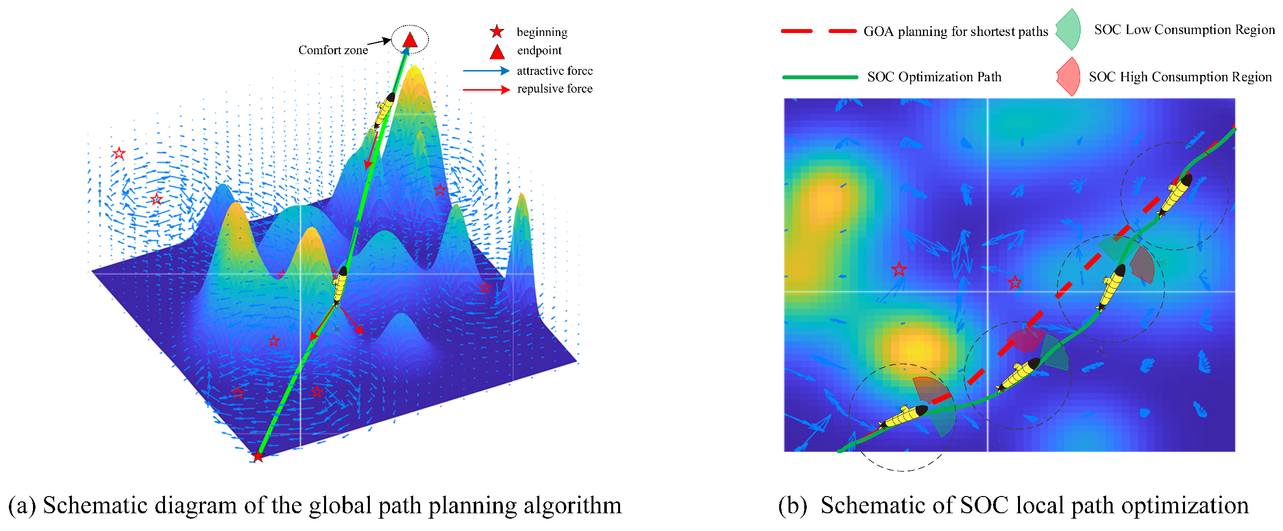
3. GOA-PF Path Planning Combined with SOC

3.1. Traditional GOA Algorithm

The Grasshopper Optimization Algorithm (GOA) [16] is an optimization algorithm that simulates the migration and predation behavior of locusts in nature and searches for the optimal food source through the interaction between individuals. In GOA, the location of a locust individual represents a candidate solution to the optimization problem. Locust individuals are mainly affected by three factors: the interaction force between locust populations, wind force, and gravity. The computational framework used for modeling locust flocking behavior is as follows:

$$X_i=S_i+G_i+A_i$$

(28)

where $X_i$ defines the location of the $i^{th}$ locust, $S_i$ signals social interaction, $G_i$ denotes the gravitational force acting over the $i^{th}$ locust and $A_i$ represents a wind force influencing a $i^{th}$ locust.

By substituting each component into the Formula (28), we can obtain the following:

$$X_i=\sum _{\begin{array}{c}j=1\\ j\ne i\end{array}}^{N}s\left(d_{ij}\right){\mathbf{d}}_{ij}-g{e}_{\mathrm{g}}-p{e}_{\mathrm{w}}$$

(29)

This mathematical model is not immediately applicable to solving the optimization problem, primarily because locusts rapidly attain their comfort zone, preventing the swarm from converging to the designated site. The optimization problem is reformulated as follows:

$$X_i^d=c\sum _{\begin{array}{c}j=1\\ j\ne i\end{array}}^N\left(c{\displaystyle \frac{{\mathrm{ub}}_d-{\mathrm{lb}}_d}{2}}s\left(d_{ij}\right){\mathbf{d}}_{ij}\right)+T_d$$

(30)

where N represents the population size, $u{b}_d$ specifies the upper limit of the target’s d-th depth, $l{b}_d$ signifies the smaller limit of the d-th depth, and $T_d$ indicates the optimal value of the d-th dimension for the destination; c is the coefficient for the linear reduction of the soothing zone, repulsion zone, and attractiveness zone. This formula disregards the impact of gravity and presumes that the wind direction consistently aligns with the ideal solution. The representation of c is as follows:

$$C=C_{max}-n{\displaystyle \frac{C_{max}-C_{min}}{L}}$$

(31)

where n is the current number of repetitions, L represents the maximum permitted amount of repetitions, as well as the parameters $c_{max}$ and $c_{min}$ are 1 and 0.0004, respectively.

During the entire algorithm iteration process, the evaluation index of the quality of each locust position is the fitness function. For mobile robot path planning, the fitness function is usually adopted to satisfy the shortest moving path. The ideal solution to the problem is achieved by iteratively applying Formula (36) during the solution process. The ideal solution for the current problem is documented as the highest fitness value achieved after each iteration, continuing until the maximum iteration limit is attained.

3.2. GOA-PF Path Planning Algorithm Combined with SOC

The efficacy of the GOA, being a heuristic algorithm, is significantly influenced by the initial population value. In GOA, the initialization of the population is determined randomly. This method is prone to the uneven distribution of the population in the solution space, and there may be a phenomenon of population aggregation, which may affect the convergence of the next step. In order to prevent the population from being too dense and causing unnecessary energy loss, the APF algorithm is introduced to optimize the local energy of the SOC. The APF algorithm is a widely utilized local route planning technique characterized by its straightforward mathematical formulation, low computer cost, rapid response time, and smooth trajectory generation. The flowchart of the path planning algorithm is illustrated in Figure 4. Improvements have been implemented in the APF algorithm based on the research. In the local optimization stage, the SOC change of each path point on the global path is calculated based on the energy consumption model. The path points with large SOC changes are regarded as high energy consumption points (repulsive force points), and the path points with small SOC changes are regarded as low energy consumption points (attractive points). The gravitational and repulsive fields are constructed in combination with the APF algorithm, and the global path is locally adjusted to optimize the energy consumption distribution. Figure 5 shows a schematic of the algorithm. The pseudo-code of the algorithm is shown in Algorithm 1.

The SOC reference trajectory is introduced and defined as $SO{C}_{ref}\left(t\right)$ to guide path selection and maintain SOC in the ideal range. The trajectory is designed to gradually decrease with the path length in order to balance the SOC consumption during the entire mission:

$$SO{C}_{ref}\left(t\right)=SO{C}_{max}-\left({\displaystyle \frac{SO{C}_{max}-SO{C}_{min}}{L_{total}}}\right)·D\left(t\right)$$

(32)

where $SO{C}_{max}$ and $SO{C}_{min}$ are the initial SOC rating and the lowest permissible SOC value of the battery; $L_{total}$ is the projected total path length; $D\left(t\right)$ represents the length of the traveled path at the present instant.

The formulas for attracting and repulsive forces are as follows:

$$U_{att}\left(x\right)={\displaystyle \frac{1}{2}}\zeta \left(1+k·\left(SOC\left(t\right)-{\mathrm{SOC}}_{ref}\right)\right){∥x-x_{\mathrm{goal}}∥}^2$$

(33)

$$U_{rep}\left(x\right)=\left\{\begin{array}{cc}{\displaystyle \frac{1}{2}}\eta {\left({\displaystyle \frac{1+m·(SOC-{\mathrm{SOC}}_{ref})}{\Vert x-x_{\mathrm{obs}}\Vert }}-{\displaystyle \frac{1}{d_{\mathrm{safe}}}}\right)}^2\hfill & \mathrm{if}\Vert x-x_{\mathrm{obs}}\Vert \le d_{\mathrm{safe}}\hfill \\ 0\hfill & \mathrm{if}\Vert x-x_{\mathrm{obs}}\Vert >d_{\mathrm{safe}}\hfill \end{array}\right.$$

(34)

In the formula, $\zeta$ and $\eta$ are the basic attraction coefficient and repulsion gain coefficient of the AUV’s position, and k is the SOC attraction factor. When the SOC deviates from the reference value, the attraction is increased to reduce the additional path consumption; m is the repulsion influence factor. When the SOC is low, the repulsion force increases, enhancing the obstacle avoidance ability and thereby reducing emergency acceleration and high-energy maneuvers. By solving the gradients of the attraction and repulsion potential fields, the equation of the total potential field force is formulated as follows:

$$U\left(x\right)=\sum _{i=1}^m{U}_{att}\left(x_i\right)+\sum _{j=1}^n{U}_{rep}\left(x_j\right)$$

(35)

$$F_{att}\left(x\right)=-\nabla U_{att}\left(x\right)=-\zeta (1+k·(SOC-{\mathrm{SOC}}_{ref}))(x-x_{\mathrm{goal}})$$

(36)

$$F_{rep}\left(x\right)=\nabla U_{rep}\left(x\right)$$

(37)

$$F=F_{att}\left(x\right)+F_{rep}\left(x\right)$$

(38)

where F represents the total potential field derived from the summation of the repulsive and attractive fields, followed by the computation of the gradient of the resultant field to ascertain the vehicle’s direction of travel.

In order to ensure that the proposed GOA-PF path planning algorithm and SOC-optimized MPC trajectory tracking controller can be practically applied in real-time control tasks, this section provides an analysis of the computational complexity and real-time performance of both algorithms. The GOA-PF path planning algorithm combines the GOA with the APF method to achieve global path planning and local path optimization. The time complexity of the GOA-PF algorithm can be derived from the following components:

Global Path Planning: The GOA algorithm uses a population for global search, and assuming the population size is n and the number of iterations is T, and the time complexity is $O(n·T)$.

Local Path Optimization: The APF algorithm optimizes the path locally. Its complexity depends on the number of path nodes m and the number of local iterations k, so the time complexity is $O(m·k)$.

Thus, the overall time complexity of the GOA-PF algorithm is $O(n·T+m·k)$. As the complexity of the environment increases (e.g., more obstacles, longer paths), the complexity of the algorithm will increase, but it still maintains an acceptable performance under reasonable task scales.

In terms of space complexity, the GOA algorithm requires memory to store the population, where each individual requires storage for p parameters (e.g., position, velocity), so the space complexity is $O(n·p)$.

Algorithm 1: Pseudocode of GOA-PF algorithm combined with SOC optimization

Input: ${\mathbf{P}}_{\mathrm{start}}$, ${\mathbf{P}}_{\mathrm{goal}}$, Environment data, Initial SOC

Output: ${\mathbf{P}}_{\mathrm{final}}$

1: Initialize population ${\mathbf{X}}_i(i=1,2,\dots ,N)$ in search space 2: for $t=1$ to MaxIterations do 3:     Evaluate $F_{\mathrm{path}}\left({\mathbf{X}}_i\right)$ for all individuals 4:     Update ${\mathbf{X}}_i$ using GOA rules 5:     Update global best path ${\mathbf{P}}_{\mathrm{global}}$ 6: end for 7: Compute $\Delta {\mathrm{SOC}}_i$ for all points in ${\mathbf{P}}_{\mathrm{global}}$ 8: for each point in ${\mathbf{P}}_{\mathrm{global}}$ do 9:    if $\Delta {\mathrm{SOC}}_i>{\mathrm{threshold}}_{\mathrm{high}}$ then 10:        Mark as repulsion point 11:    else if $\Delta {\mathrm{SOC}}_i<{\mathrm{threshold}}_{\mathrm{low}}$ then 12:        Mark as attraction point 13:    end if 14: end for 15: Adjust ${\mathbf{P}}_{\mathrm{global}}$ using artificial potential field to obtain ${\mathbf{P}}_{\mathrm{optimized}}$ 16: Return ${\mathbf{P}}_{\mathrm{final}}={\mathbf{P}}_{\mathrm{optimized}}$

4. Design of MPC Controller Based on SOC Optimization

This part mainly investigates the three-dimensional path tracking problem of AUV in challenging marine environments [36]. According to the reference path planned in the previous chapter, the dynamic characteristics of the underwater robot are controlled to keep its position consistent. As shown in Figure 6, MPC control is employed to facilitate the gradual convergence of the AUV’s driving position to the specified command while minimizing SOC consumption, guaranteeing that the AUV position tracking error converges and the SOC is managed to decrease appropriately. Taking into account the relevant limitations during the design of each controller can more efficiently identify the ideal solution within the control set.

4.1. MPC Controller Design

In this study, the complete AUV model is formulated by combining the nonlinear six-degree-of-freedom (6-DOF) dynamic equations of motion with the corresponding kinematic equations (as given in Equation (8)). Because AUV missions are typically executed around a balanced attitude (trim condition) and at moderate speeds, the nonlinear state-space model can be linearized about a suitable equilibrium operating point to simplify controller design. In this linearization process, the restoring force term $g\left(\eta \right)$ is set to zero (assuming the AUV is neutrally buoyant in a level posture) and the ocean current disturbance is neglected. As a result, a continuous-time linear time-invariant state-space model is obtained, which is then discretized to serve as the predictive model for the MPC controller design.

The vector $\mathbf{x}={\left[\begin{array}{cc}{\eta }^T& {\nu }^T\end{array}\right]}^T\in {\mathbb{R}}^{12}$ is defined as a state vector, including the starting point component $\eta$ and the vector of velocity $\nu$. A complex status space description for an underwater robot is built by merging kinematics and dynamics.

$$\begin{array}{cc}\hfill \dot{\mathbf{x}}& ={\mathbf{A}}_c\left(\mathbf{x}\right)+{\mathbf{B}}_c\tau +{\mathbf{D}}_c{\tau }^w\hfill \\ \hfill \mathbf{y}& =\mathbf{G}\mathbf{x}\hfill \end{array}$$

(39)

where

$${\mathbf{A}}_c\left(\mathbf{x}\right)=\left[\begin{array}{cc}\mathbf{0}& \mathbf{J}\left(\eta \right)\\ \mathbf{0}& -{\mathbf{M}}^{-1}(\mathbf{C}\left({\nu }^r\right)+\mathbf{D}\left({\nu }^r\right))\end{array}\right]\mathbf{x}-\left[\begin{array}{c}\mathbf{0}\\ {\mathbf{M}}^{-1}\left(\mathbf{g}\left(\eta \right)\right)\end{array}\right]$$

$${\mathbf{D}}_c={\mathbf{B}}_c=\left[\begin{array}{c}\mathbf{0}\\ {\mathbf{M}}^{-1}\end{array}\right]$$

$$\mathbf{G}=\left[\begin{array}{cc}\mathbf{I}& 0\end{array}\right]$$

and $\mathbf{y}=\eta \in {\mathbb{R}}^6$ be the result column. ${\tau }^w$ depicts the forces and moments caused by ocean currents that influence the motion of the AUV. Constraints are imposed around the location vector $\eta$ to prevent exceptional conversion matrices $J\left(\eta \right)$. Furthermore, considering that the bulk of missions are conducted at very moderate velocities, it is preferable to impose an upper limit on the linear speed of the underwater vehicle. Consequently, the restriction collection for the condition vector X is demarcated as follows:

$$X=\left\{\mathbf{x}\in {\mathbb{R}}^{12}:\mid \mathbf{x}\mid \le {\mathbf{x}}_{max}\right\}$$

(40)

The constantly changing linear model in (39) is streamlined by establishing $g\left(\eta \right)=0$, neglecting unidentified currents and waves, and discretized using the backward Euler method to obtain a model of state space for controller construction.

$$\begin{array}{cc}\hfill \mathbf{x}(\kappa +1)& =A_x\mathbf{x}\left(\kappa \right)+B\tau \left(\kappa \right)\hfill \\ \hfill \mathbf{y}\left(\kappa \right)& =C_{\mathrm{x}}\mathbf{x}\left(\kappa \right)\hfill \end{array}$$

(41)

where

$$A_x=\left[\begin{array}{cc}\mathbf{I}& \mathbf{J}\left(\eta \right)T_s\\ \mathbf{0}& (\mathbf{I}-{\mathbf{M}}^{-1}(\mathbf{C}\left(\nu \right)+\mathbf{D}\left(\nu \right)))T_s\end{array}\right]$$

$$B=\left[\begin{array}{c}\mathbf{0}\\ {\mathbf{M}}^{-1}{T}_s\end{array}\right]C_{\mathrm{x}}=\left[\begin{array}{cc}I& 0\end{array}\right]$$

where $T_s$ denotes the sample period and $\kappa$ represents the duration number. For clarity, the duration indices from $\eta$ and $\nu$ are removed for the equation of $A_x$ since they pertain to the time indices of $\mathbf{x}\left(\kappa \right)$.

Assume that all states are measurable. Let $N_p$ be the prediction time domain, $N_c$ be the control time domain, and $N_c\le N_p$. Define $Y_v$ as the output vector predicted in $N_p$ steps, and define $\Delta U$ as the input vector in $N_c$ steps:

$$Y=\left[\begin{array}{c}y(\kappa +1\mid \kappa )\\ y(\kappa +2\mid \kappa )\\ ⋮\\ y(\kappa +N_p\mid \kappa )\end{array}\right]$$

(42)

$$\Delta U=\left[\begin{array}{c}\mathit{\tau }\left(\kappa \right)\\ \mathit{\tau }(\kappa +1)\\ ⋮\\ \mathit{\tau }(\kappa +N_c-1)\end{array}\right]$$

(43)

In accordance with the model predictive control concept, the prediction equation expression could be generated as follows:

$$Y=S_{x}x\left(\kappa \right)+S_u\Delta U$$

(44)

where

$$S_x={\left[\begin{array}{cccc}{C}_x{A}_x& C_x{A}_x^2& \dots & C_x{A}_x^{N_p}\end{array}\right]}^T$$

$$S_u=\left[\begin{array}{cccc}{C}_{x}B& 0& ...& 0\\ C_x{A}_{x}B& C_x{B}_x& ...& 0\\ ⋮& ⋮& \ddots & ⋮\\ C_x{A}_x^{N_p-1}B& C_x{A}_x^{N_p-2}B& ...& C_x{A}_x^{N_p-N_c}B\end{array}\right]$$

In controller design, the system status $x\left(\kappa \right)$ with the control input $\tau \left(\kappa \right)$ serve as constraints. The system state $x\left(\kappa \right)$ is confined by an upward and downward bound, and the control system input $\tau \left(\kappa \right)$ is likewise finite.

$$x{\left(\kappa \right)}_{min}\le x\left(\kappa \right)\le x{\left(\kappa \right)}_{max}$$

(45)

$$\mathit{\tau }{\left(\kappa \right)}_{min}\le \mathit{\tau }\left(\kappa \right)\le \mathit{\tau }{\left(\kappa \right)}_{max}$$

(46)

where $x{\left(\kappa \right)}_{min}$, $\tau {\left(\kappa \right)}_{min}$ are predefined lower limits, and $x{\left(\kappa \right)}_{max}$, $\tau {\left(\kappa \right)}_{max}$ are predefined upper limits. The present state of the system’s $x\left(\kappa \right)$ constraints is converted into control input increment $\Delta u\left(\kappa \right)$ constraints and expressed as the following compact linear constraint forms:

$$M\Delta U_{\le }\gamma$$

(47)

where

$$M=\left[\begin{array}{c}I\\ B\end{array}\right]\gamma =\left[\begin{array}{c}\Delta U_{\max }-\Delta U_{\min }\\ X_{\max }-A_x\left(\kappa \right)-X_{\min }+A_x\left(\kappa \right)\end{array}\right]$$

Choose a particular objective function:

$$\underset{\Delta U\left(\kappa \right)}{min}J(y\left(\kappa \right),\Delta U,N_p,N_c)=\Vert {\mathsf{\Gamma }}_y\left(Y\left(\kappa \right)\right){-\nu \left(\kappa \right)\Vert }^2+{\Vert {\mathrm{\Gamma }}_u\Delta U\left(\kappa \right)\Vert }^2$$

(48)

where ${\mathrm{\Gamma }}_y$ and ${\mathrm{\Gamma }}_u$ indicate the weighting coefficient of the output signal and the weighting factor of the control signal, respectively.

4.2. Design of MPC Controller Combined with SOC Optimization

For AUVs with limited energy resources, their path tracking control needs to take into account both trajectory accuracy and energy consumption optimization. The objective function of traditional MPC controllers usually only focuses on the output error and the change of control input, ignoring the importance of battery state of charge (SOC) to system energy management. Therefore, in order to extend the endurance of AUVs, this section introduces the SOC optimization strategy in the MPC controller design, incorporates the SOC consumption into the objective function, and imposes energy consumption constraints on the control input.

$$\Delta \mathrm{SOC}(\kappa +i)=SOC\left(\kappa \right)-{\eta }_{bat}{\displaystyle \frac{J_P(\kappa +i)·T_s}{V·C_{\mathrm{bat}}}}$$

(49)

where $J_P(\kappa +i)$ is the total power consumption predicted in the i step, including propulsion power consumption, attitude adjustment power consumption, and power resource consumption, and V and $Q_{total}$ are the battery voltage and total battery capacity.

To further optimize energy consumption, we add the following constraints in the MPC controller:

$$\begin{array}{cc}\hfill \mathsf{\Delta }{\mathrm{SOC}}_{min}& \le \mathsf{\Delta }\mathrm{SOC}(\kappa +i)\le \mathsf{\Delta }{\mathrm{SOC}}_{max}\hfill \\ \hfill {\tau }_{min}& \le \tau (\kappa +i)\le {\tau }_{max}\hfill \end{array}$$

(50)

$\Delta {\mathrm{SOC}}_{min}$ was introduced as a lower limit for the energy consumption of a single step, with the aim of ensuring that the energy consumption of each control step is not too low, thus avoiding unstable values or invalid solutions. Consequently, the goal function may be reformulated as follows:

$$\underset{\mathsf{\Delta }U\left(\kappa \right)}{min}J=\Vert {\mathsf{\Gamma }}_{y2}{\left(Y\left(\kappa \right)\right)-\nu \left(\kappa \right)\Vert }^2+\Vert {\mathsf{\Gamma }}_{u2}{\mathsf{\Delta }U\left(\kappa \right)\Vert }^2+\lambda {\Vert \mathsf{\Delta }\mathrm{SOC}(\kappa +i)\Vert }^2$$

(51)

where $\mathsf{\Delta }SOC(\kappa +i)$ is the SOC change predicted in the i step, and $\lambda$ is the weight factor of the SOC optimization term, which controls the balance between energy consumption optimization and trajectory accuracy.

Taking Y as the objective function, we can obtain the quadratic equation about $\tau \left(\kappa \right)$. The final standard convex quadratic programming form can be written as follows:

$$\begin{array}{cc}\hfill & \tau \left(\kappa \right)=\underset{\tau \left(\kappa \right)}{\mathrm{argmin}}\left({\displaystyle \frac{1}{2}}\tau {\left(\kappa \right)}^{\top }H\left(\kappa \right)\tau \left(\kappa \right)+f^{\top }\left(\kappa \right)\tau \left(\kappa \right)\right)\hfill \\ \hfill & \mathrm{s}.\mathrm{t}.M\mathsf{\Delta }U\le \gamma \hfill \end{array}$$

(52)

where

$$H\left(\kappa \right)=-\left(S_u^T{\mathsf{\Gamma }}_y^T{\mathsf{\Gamma }}_y{S}_u+{\mathsf{\Gamma }}_u^T{\mathsf{\Gamma }}_u\right)$$

(53)

$$f\left(\kappa \right)=\left(S_u^T{\mathsf{\Gamma }}_y^T{\mathsf{\Gamma }}_y\left(S_{x}x\left(\kappa \right)-\nu \left(\kappa \right)\right)\right)$$

(54)

The converted quadratic programming problem can be calculated online. Then, the optimal input vector ${\tau }^{\ast }\left(\kappa \right)$ for prediction can be obtained.

At each sample period $\kappa$, ${\tau }^{\ast }\left(\kappa \right)$ is computed to facilitate the rolling horizon optimization. The anticipated state $x(\kappa +1)$ and the ideal input ${\tau }^{\ast }\left(\kappa \right)$ are ascertained from the current state $x\left(\kappa \right)$. Therefore, MPC can compensate for the system uncertainty caused by model mismatch and external disturbances. The rolling optimization process is continuously iterated until the AUV trajectory tracking task is completed. It can be seen that MPC can reduce the impact of model uncertainty. This paper focuses on practical engineering applications, such as the impact of external disturbances and energy states on AUV trajectory tracking.

4.3. Stability Analysis

Theorem: For the MPC-based controller (41), consider the cost function (46) with constraint (47). Select the positive definite matrix ${\mathsf{\Gamma }}_y$, the positive definite matrix ${\mathsf{\Gamma }}_u$, the prediction horizon Np, and the control horizon $N_c$ and ensure that the optimal solution of the cost function (46) exists. Designate the ideal price function $J^{\ast }\left(\kappa \right)$ to be the Lyapunov function $V^{\ast }\left(\kappa \right)$. If $V^{\ast }(\kappa +1)\le V^{\ast }\left(\kappa \right)$ holds, then the optimum approach ${\tau }^{\ast }\left(\kappa \right)$ assures the theoretical equilibrium of the system (41).

Proof: In the most effective approach $\Delta U^{\ast }\left(\kappa \right)$ of the cost function (46) subject to the constraint (47), ${\tau }^{\ast }(\kappa +i|\kappa )$ is selected as the ideal increment for the control input. Thus, $x^{\ast }(\kappa +i|\kappa )$ represents the optimal control input associated with the optimal control signal increase ${\tau }^{\ast }(\kappa +i|\kappa )$. The ideal cost function $J^{\ast }\left(\kappa \right)$ is identified as the Lyapunov function $V^{\ast }\left(\kappa \right)$.

$$\begin{array}{cc}\hfill V^{\ast }\left(\kappa \right)& =minJ\left(\kappa \right)\hfill \\ \hfill & =min[\sum _{i=1}^{N_p}\parallel {\mathsf{\Gamma }}_y\left(y_{\eta }(\kappa +i|\kappa )\right)-y_d(\kappa +i|\kappa ){\parallel }^2\hfill \\ \hfill & +\sum _{i=0}^{N_c-1}\parallel {\mathsf{\Gamma }}_u\tau (\kappa +i|\kappa ){\parallel }^2+\lambda \sum _{i=1}^{N_p}\parallel \Delta \mathrm{SOC}(\kappa +i){\parallel }^2]\hfill \end{array}$$

(55)

The optimal function (52) clearly fulfills ${\mathrm{V}}^{\ast }\left(0\right)=0$, where $\kappa =0$, and ${\mathrm{V}}^{\ast }\left(\kappa \right)>0$ for any $k\ne 0$. For the system (41) subject to external disturbance, the optimal control input increment $\tau (\kappa +1+i|\kappa +1)$ and the control input $x(\kappa +1+i|\kappa +1)$ are computed as follows:

$$\begin{array}{cc}\hfill \tau (\kappa +1+i\mid \kappa +1)& =[\tau (\kappa +1\mid \kappa +1),\tau (\kappa +2\mid k+1),\dots ,\tau (\kappa +N_{c1}\mid \kappa +1)]\hfill \\ \hfill & =[{\tau }^{\ast }(\kappa +1\mid \kappa +1),{\tau }^{\ast }(\kappa +2\mid \kappa +1),\dots ,{\tau }^{\ast }(\kappa +N_c\mid \kappa +1)]\hfill \end{array}$$

(56)

$$\begin{array}{cc}\hfill x(\kappa +1+i\mid \kappa +1)& =[x(\kappa +1\mid \kappa +1),x(\kappa +2\mid \kappa +1),\dots ,x(\kappa +N_{c1}\mid \kappa +1)]\hfill \\ \hfill & =[x^{\ast }(\kappa +1\mid \kappa +1),x^{\ast }(\kappa +2\mid \kappa +1),\dots ,x^{\ast }(\kappa +N_c\mid \kappa +1)]\hfill \end{array}$$

(57)

It is straightforward to demonstrate that (53) and (54) constitute feasible solutions to the quadratic programming problem (49). The control increment $\tau (\kappa +1+i|\kappa +1)$ and the controller $x(\kappa +1+i|\kappa +1)$ adhere to the restrictions (45), (46), and (50), respectively. Furthermore, owing to the optimality of the cost function (27), the function $J(\kappa +1)$ is not inferior to $V^{\ast }(\kappa +1)$.

$$V^{\ast }(\kappa +1)\le V^{\ast }\left(\kappa \right)$$

(58)

Consequently, the correlation among $V^{\ast }\left(\kappa \right)$ with $J(\kappa +1)$ is demarcated in the following manner:

$$\begin{array}{cc}\hfill V^{\ast }(\kappa +1)& \le J(\kappa +1)\hfill \\ \hfill & \le V^{\ast }\left(\kappa \right)-\parallel {\mathsf{\Gamma }}_y\left(y_{\eta }^{\ast }\left(\kappa \right)\right)-y_d{\left(\kappa \right)\parallel }^2-\parallel {\mathsf{\Gamma }}_u{\tau }^{\ast }{\left(\kappa \right)\parallel }^2+\lambda {\parallel \Delta \mathrm{SOC}(\kappa +i)\parallel }^2\hfill \end{array}$$

(59)

For $\kappa =0$, the Lyapunov function (61) fulfills $V^{\ast }\left(0\right)=0$, whereas for any $\kappa \ne 0$, $V^{\ast }\left(\kappa \right)>0$. The Lyapunov function (61) is monotonically non-increasing, namely, $V^{\ast }(\kappa +1)\le V^{\ast }\left(\kappa \right)$. Consequently, the system (47) exhibits nominal stability.

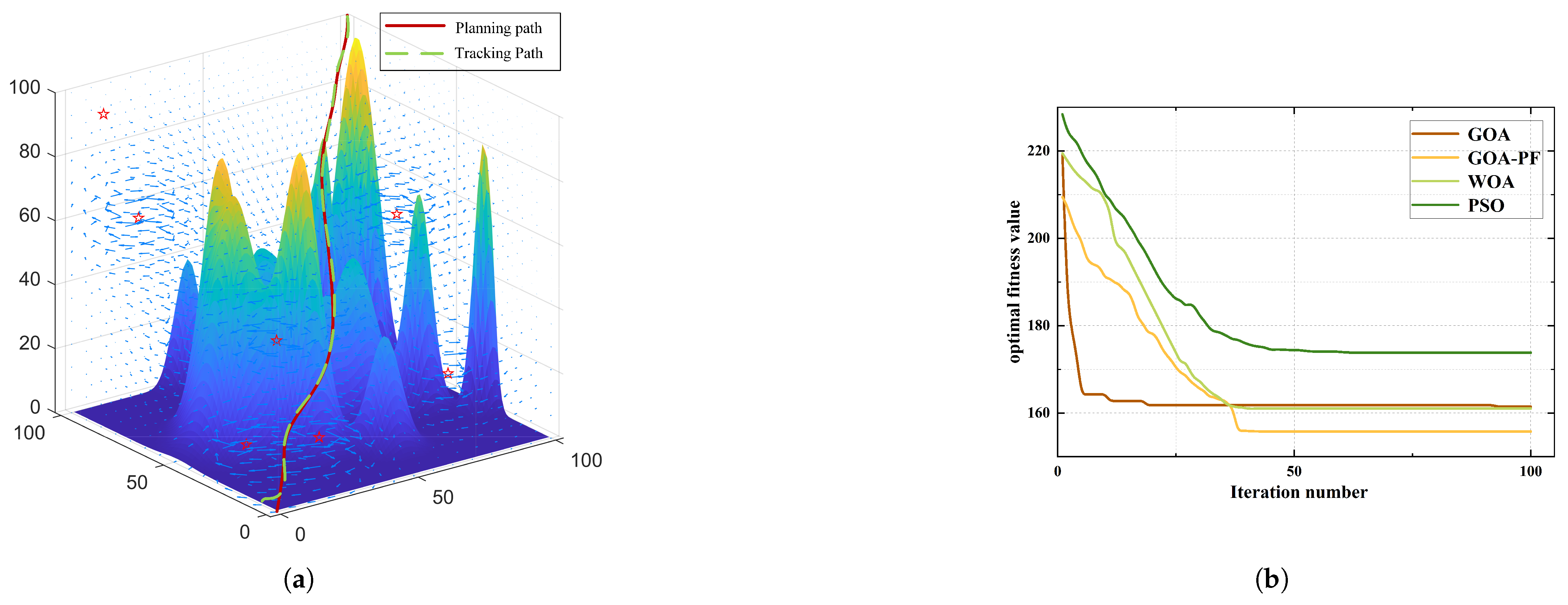
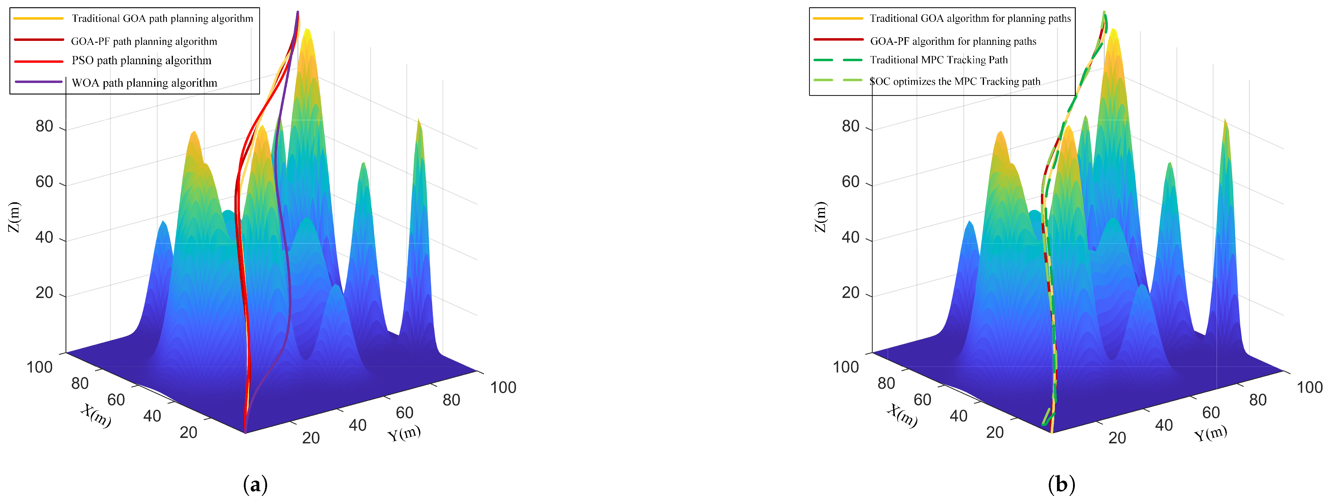
5. Simulation Results Analysis

This section validates the efficacy of the SOC-optimized path planning and trajectory tracking framework through extensive simulations. The experiments demonstrate the collaborative optimization of path planning and tracking, analyze the dynamic management of SOC consumption, and test the framework’s robustness under complex environments. The GOA-PF algorithm with SOC optimization is employed for path planning, while an SOC-optimized MPC controller ensures precise tracking of the planned path. By comparing with traditional methods, key metrics such as path length, tracking error, and SOC consumption are analyzed to highlight the advantages of the proposed framework in energy efficiency.

5.1. Path Planning and Tracking Control Results

In this experiment, we used a standard simulation platform for testing. The hardware platform used for the experiment is a laptop computer with an Intel i7 processor, and the runtime environment is the standard MATLAB 2024a simulation environment. We tested the computational performance of the whole system (including path planning, control optimization and SOC estimation) in a typical AUV task scenario. The simulation task contains path planning, trajectory tracking, and battery SOC monitoring.

In our experiments, we measured the total computation time for each control loop. Below is the average computation time for each part of the algorithm:

GOA-PF path planning: using a population size of 50 and an iteration number of 100 setup, the average computation time is 40 ms.

SOC-MPC control: the average computation time to solve the quadratic optimization problem is 45 ms with a prediction time domain of 20 steps.

Based on these results, the total computation time for each control cycle of the whole system is about 85 ms. Considering that the control frequency of the AUV is 10 Hz (i.e., the control command is updated every 0.1 s), this computation time fully satisfies the real-time control requirements.

Table 1. AUV Related Parameters.

Parameters	Value	Parameters	Value
m	185 kg	$Y_v$	100 kg/s
$X_{\dot{u}}$	$-30$ kg	$Y_{\left|v\right|v}$	200 kg/m
$Y_{\dot{v}}$	$-80$ kg	$Z_w$	100 kg/s
$Z_{\dot{w}}$	$-80$ kg	$Z_{\left|w\right|w}$	200 kg/m
$I_y$	40 kgm2	$M_q$	50 kgm2/($\mathrm{s}·$rad)
$M_{\dot{q}}$	$-40$ kgm2	$M_{\left|q\right|q}$	100 kgm2/rad
$I_z$	40 kgm2	$N_r$	50 kgm2/($\mathrm{s}·$rad)
$N_{\dot{r}}$	$-40$ kgm2	$N_{\left|r\right|r}$	100 kgm2/rad
$X_u$	70 kg/s	$X_{\left|u\right|u}$	100 kg/m
$k_{t1}$	−0.2896	$k_{q1}$	0.0084
$k_{t2}$	−0.1114	$k_{q2}$	0.0283
$k_{t3}$	0.5420	$k_{q3}$	0.0947
$\epsilon$	0.0274	D	10 N·s/m

and

Table 2. Path planning and trajectory control parameters.

Parameters	Value
$T_s$	0.2 s
$N_p$	50
$N_c$	5
${\mathsf{\Gamma }}_{y2}$	$diag[0.1,0.1,0.1,0.1,0.1,0.1,0.1]$
${\mathsf{\Gamma }}_{u2}$	$diag[1,1,1,1,1,1]$
$c_{max}$	1
$c_{min}$	0.004
l	1.5
f	0.5

give the parameters related to the studied AUVs and the design of the control algorithm, respectively. The initial state defined is by the simulation is (0, 0, 0). The end point is (100, 100, 100). AUV geopotential avoidance and current perturbations are randomly generated according to (11) and (12). The initial state of AUV trajectory tracking is ${[6,3,0,0,0,0]}^T$. In this Section 5.1, the simulation results of the AUV apply the proposed framework by presetting various parameters of the AUV, Figure 7a demonstrates the effect of planning the path and tracking control in the SOC-optimized seafloor terrain and current environment, which bypasses the mountain while searching for the SOC-optimal path as much as possible, and finally arrives at the preset target point from the starting point. Figure 7b shows the fitness value of the GOA-PF algorithm with the traditional GOA algorithm, Particle Swarm Algorithm (PSO), Whale Optimization Algorithm (WOA) at 100 iterations; the GOA-PF optimization algorithm has obtained the best fitness value after weighing the shortest path with SOC reasonable descent. Compared to other algorithms, although the convergence speed is not the fastest, the convergence accuracy is also the best, which indicates that the GOA-PF optimization algorithm has a stronger patrolling optimization ability for path and SOC descent as well as overall stability.

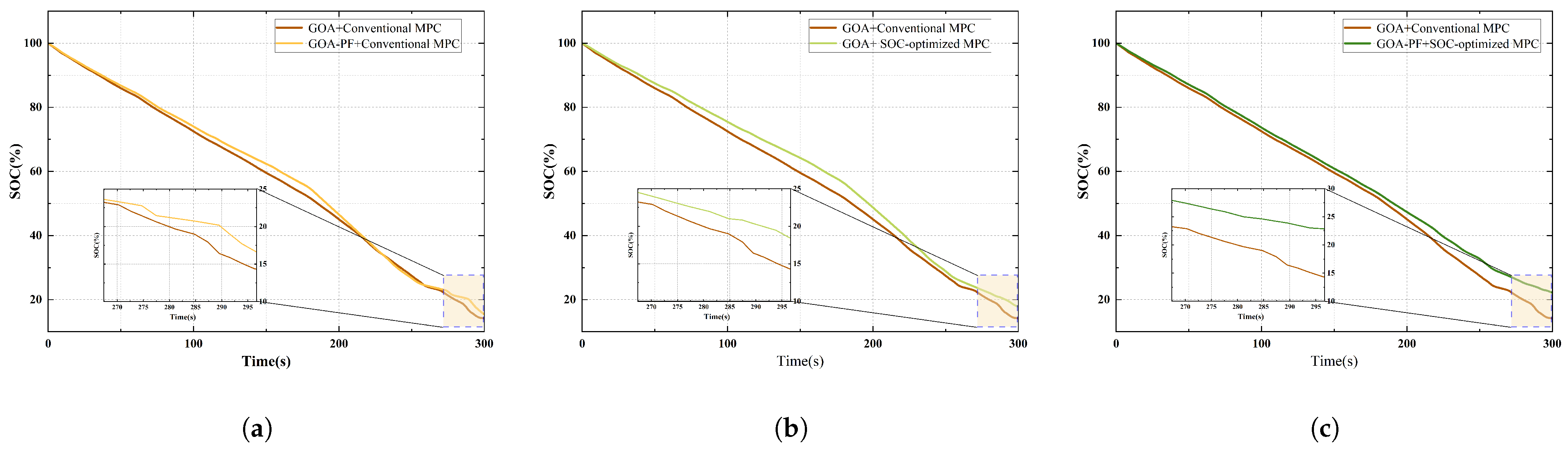
5.2. Comparative Analysis Without Perturbation

In order to verify the reasonableness of the established model and the effectiveness of the GOA-PF algorithm as well as the overall optimization capability, the GOA-PF algorithm is compared with the classical particle swarm optimization algorithm (PSO), the traditional locust optimization algorithm (GOA), and the whale optimization algorithm (WOA) for the planning of paths. For each algorithm, the control parameters are representative empirical values and are derived from the original article. The GOA-PF algorithm searches for the global optimal path based on the locust optimization algorithm to find the lowest local SOC consumption with the APF to construct the gravitational and repulsive fields in order to optimize the energy consumption. The four optimization algorithms paths are shown in Figure 8a. Figure 8b shows the path planning and trajectory tracking results of the seafloor topography in the absence of current perturbation. As shown, the yellow and red solid lines indicate the paths planned by the conventional GOA algorithm and the GOA-PF algorithm, respectively, while the two dashed lines indicate the trajectory tracking paths traveled by the conventional MPC as well as the SOC-optimized MPC controller. In the absence of current perturbations, the traditional algorithm and the algorithm designed in the article yield roughly the same results, and due to the absence of perturbations, the algorithms both travel the shortest path possible to minimize SOC consumption.

Figure 9 shows the position tracking error comparison results of different algorithms, using the traditional planning and trajectory control algorithms, respectively, with the path planning algorithm of the SOC optimization framework and trajectory tracking algorithms for variable-by-variable comparisons; the three graphs show that there is a small magnitude of overshooting error at the initial stage of tracking, and then the error tends to zero. Figure 10 shows the SOC under different algorithms degradation. Also, using the variable-by-variable method for comparative analysis, the SOC optimization framework consumes roughly the same SOC as the traditional algorithm in the absence of current interference.

5.3. Comparative Analysis with Perturbation

In the environment with random current disturbance, the path planning from the starting point to the end point as well as the path tracking control should not only avoid the obstacles of the seabed terrain, but also consider the impact of random currents on the SOC consumption, which is introduced into the stochastic current model according to Equation (12), and similarly, the GOA-PF algorithm will be compared to the classical particle swarm optimization algorithm (PSO), the traditional locust optimization algorithm (GOA), as well as the whale optimization algorithms for planning paths, as shown in Figure 11a. Figure 11b shows the path planning and trajectory tracking results of the traditional method and the method in the presence of current disturbances it can be found that the traditional GOA algorithm and the proposed algorithm plan different paths, and the two tracking algorithms also converge to the planned paths in a very short time to achieve an accurate trajectory tracking. Figure 12 and Figure 13 show the position tracking error and SOC consumption under current disturbances. Combined with the path lengths traveled under the different planning algorithms given in

Table 3. Different path planning algorithms and path lengths in different environments.

Algorithm	Path Lengths Under Different Algorithms Without Ocean Currents (m)	Path Lengths Under Different Algorithms for the Ocean Current Case (m)
GOA	205.14	206.32
PSO	206.89	207.51
WOA	210.13	209.86
GOA-PF	208.11	221.83

. Compared with the traditional algorithm, the proposed SOC energy optimization framework travels 7.6 percent more, but achieves an energy trade-off by deliberately bypassing the countercurrent area and taking advantage of favorable fluid dynamic conditions. This targeted flow avoidance mechanism reduces SOC consumption by 8.04 percent by optimizing propulsion efficiency, thus offsetting the extended sailing distance with stronger energy savings.

6. Conclusions

In this paper, a new control framework combined with SOC optimization is proposed to address the problem of energy management in the planning and tracking of the paths of autonomous underwater vehicles (AUVs). The efficacy of path planning in AUV missions inside intricate underwater settings directly influences the vehicle’s energy efficiency, while the precision of trajectory tracking impacts mission reliability and the rationality of energy consumption. However, traditional path planning and control methods mostly aim at the shortest path length or the strongest obstacle avoidance capability, with less consideration of energy management, especially under real working conditions, ignoring the dual effects of current interference, kinetic constraints, and battery SOC status on path selection and trajectory control. To this end, this paper firstly establishes a six-degree-of-freedom model of an underdriven AUV based on kinematics and dynamics, establishes an ocean current model as well as a seafloor geopotential model in order to characterize the dynamics constraints, and establishes a SOC state estimation model based on the ansatz-integral method. Then, the GPA-PF path planning algorithm based on the overall SOC optimization framework and the MPC trajectory tracking controller combined with SOC optimization is designed, respectively. On the basis of the GOA global path planning algorithm, the local paths are optimized based on SOC by combining with the APF algorithm, and the precision and energy efficiency of path execution are further improved by the MPC trajectory tracking controller, which realizes the deep coupling of path planning and energy management. Simulation results show that the GOA-PF framework proposed in this paper exhibits significant advantages in terms of path length, obstacle avoidance capability, and SOC optimization, and compared with the traditional GOA algorithm, the energy distribution of the planned path is more uniform, and the total SOC consumption is significantly reduced, while the trajectory tracking error is effectively suppressed. The research in this paper provides an effective solution for energy-efficient navigation of AUVs in complex underwater environments and also expands the research field of path planning and trajectory tracking based on SOC optimization. Future research efforts will focus on the following aspects: first, validating the engineering applicability of the framework through real-world underwater experiments; second, introducing real-time SOC feedback into the controller design to improve the real-time performance of energy optimization; third, exploring the application in multi-AUV collaborative tasks and investigating its scalability in group coordination and energy management; fourth, combining more advanced energy management systems, such as the hybrid energy model, to further optimize the range of AUVs.

References

1. Sahoo, A.; Dwivedy, S.K.; Robi, P. Advancements in the field of autonomous underwater vehicle. Ocean. Eng. 2019, 181, 145–160. [Google Scholar] [CrossRef]
2. Fenucci, D.; Fanelli, F.; Consensi, A.; Salavasidis, G.; Pebody, M.; Phillips, A.B. A multi-platform Guidance, Navigation and Control system for the autosub family of Autonomous Underwater Vehicles. Control. Eng. Pract. 2024, 146, 105902. [Google Scholar] [CrossRef]
3. Heshmati-Alamdari, S.; Nikou, A.; Dimarogonas, D.V. Robust trajectory tracking control for underactuated autonomous underwater vehicles in uncertain environments. IEEE Trans. Autom. Sci. Eng. 2020, 18, 1288–1301. [Google Scholar] [CrossRef]
4. Piskur, P.; Szymak, P.; Przybylski, M.; Naus, K.; Jaskólski, K.; Żokowski, M. Innovative energy-saving propulsion system for low-speed biomimetic underwater vehicles. Energies 2021, 14, 8418. [Google Scholar] [CrossRef]
5. Wang, Z.; Xiang, X.; Duan, Y.; Yang, S. Adversarial deep reinforcement learning based robust depth tracking control for underactuated autonomous underwater vehicle. Eng. Appl. Artif. Intell. 2024, 130, 107728. [Google Scholar] [CrossRef]
6. Liu, Z.; Ning, D.; Hou, J.; Zhang, F.; Liang, G. AUV path planning in a three-dimensional marine environment based on a novel multiple swarm co-evolutionary algorithm. Appl. Soft Comput. 2024, 164, 111933. [Google Scholar] [CrossRef]
7. Wen, J.; Dai, H.; He, J.; Sun, L.; Gao, L. Intelligent Decision-Making Method for AUV Path Planning Against Ocean Current Disturbance Via Reinforcement Learning. IEEE Internet Things J. 2024, 11, 38965–38975. [Google Scholar] [CrossRef]
8. Eimeni, S.N.H.; Khosravi, A. An Online Energy Management System Based on Minimum-Time Speed Planning for Autonomous Underwater Vehicles. IEEE Trans. Intell. Veh. 2024, 1–12. [Google Scholar] [CrossRef]
9. Panda, J. Machine learning for naval architecture, ocean and marine engineering. J. Mar. Sci. Technol. 2023, 28, 1–26. [Google Scholar] [CrossRef]
10. Panda, J.P.; Mitra, A.; Warrior, H.V. A review on the hydrodynamic characteristics of autonomous underwater vehicles. Proc. Inst. Mech. Eng. Part J. Eng. Marit. Environ. 2021, 235, 15–29. [Google Scholar] [CrossRef]
11. Li, L.; Li, Y.; Wang, Y.; Xu, G.; Wang, H.; Gao, P.; Feng, X. Multi-AUV coverage path planning algorithm using side-scan sonar for maritime search. Ocean Eng. 2024, 300, 117396. [Google Scholar] [CrossRef]
12. Sun, M.; Xiao, X.; Luan, T.; Zhang, X.; Wu, B.; Zhen, L. The path planning algorithm for UUV based on the fusion of grid obstacles of artificial potential field. Ocean Eng. 2024, 306, 118043. [Google Scholar] [CrossRef]
13. Xu, Z.; Shen, Y.; Xie, Z.; Liu, Y. Research on Autonomous Underwater Vehicle Path Optimization Using a Field Theory-Guided A* Algorithm. J. Mar. Sci. Eng. 2024, 12, 1815. [Google Scholar] [CrossRef]
14. Gong, Y.J.; Huang, T.; Ma, Y.N.; Jeon, S.W.; Zhang, J. Mtrajplanner: A multiple-trajectory planning algorithm for autonomous underwater vehicles. IEEE Trans. Intell. Transp. Syst. 2023, 24, 3714–3727. [Google Scholar] [CrossRef]
15. Wen, J.; Yang, J.; Wang, T. Path planning for autonomous underwater vehicles under the influence of ocean currents based on a fusion heuristic algorithm. IEEE Trans. Veh. Technol. 2021, 70, 8529–8544. [Google Scholar] [CrossRef]
16. Saremi, S.; Mirjalili, S.; Lewis, A. Grasshopper optimisation algorithm: Theory and application. Adv. Eng. Softw. 2017, 105, 30–47. [Google Scholar] [CrossRef]
17. Mirjalili, S.Z.; Mirjalili, S.; Saremi, S.; Faris, H.; Aljarah, I. Grasshopper optimization algorithm for multi-objective optimization problems. Appl. Intell. 2018, 48, 805–820. [Google Scholar] [CrossRef]
18. Ingle, K.K.; Jatoth, R.K. Non-linear channel equalization using modified grasshopper optimization algorithm. Appl. Soft Comput. 2024, 153, 110091. [Google Scholar] [CrossRef]
19. Yan, Z.; Yan, J.; Wu, Y.; Cai, S.; Wang, H. A novel reinforcement learning based tuna swarm optimization algorithm for autonomous underwater vehicle path planning. Math. Comput. Simul. 2023, 209, 55–86. [Google Scholar] [CrossRef]
20. Liang, X.; Dong, Z.; Hou, Y.; Mu, X. Energy-saving optimization for spacing configurations of a pair of self-propelled AUV based on hull form uncertainty design. Ocean Eng. 2020, 218, 108235. [Google Scholar] [CrossRef]
21. Li, B.; Gao, X.; Huang, H.; Yang, H. Improved adaptive twisting sliding mode control for trajectory tracking of an AUV subject to uncertainties. Ocean Eng. 2024, 297, 116204. [Google Scholar] [CrossRef]
22. Sun, Y.; Du, Y.; Qin, H. Distributed adaptive neural network constraint containment control for the benthic autonomous underwater vehicles. Neurocomputing 2022, 484, 89–98. [Google Scholar] [CrossRef]
23. Tang, J.; Dang, Z.; Deng, Z.; Li, C. Adaptive fuzzy nonlinear integral sliding mode control for unmanned underwater vehicles based on ESO. Ocean Eng. 2022, 266, 113154. [Google Scholar] [CrossRef]
24. Yang, N.; Chang, D.; Amini, M.R.; Johnson-Robersor, M.; Sun, J. Energy management for autonomous underwater vehicles using economic model predictive control. In Proceedings of the 2019 American Control Conference (ACC), Philadelphia, PA, USA, 10–12 July 2019; pp. 2639–2644. [Google Scholar] [CrossRef]
25. Miao, J.; Wang, Y.; Deng, K.; Sun, X.; Liu, W.; Guo, Z. PECLOS path-following control of underactuated AUV with multiple disturbances and input constraints. Ocean Eng. 2023, 284, 115236. [Google Scholar] [CrossRef]
26. Esmaiel, H.; Sun, H. Energy Harvesting for TDS-OFDM in NOMA-Based Underwater Communication Systems. Sensors 2022, 22, 5751. [Google Scholar] [CrossRef]
27. Mostafa, M.; Esmaiel, H.; Omer, O.A. Hybrid energy efficient routing protocol for UWSNs. In Proceedings of the 2020 2nd International Conference on Computer and Information Sciences (ICCIS), Sakaka, Saudi Arabia, 13–15 October 2020; pp. 1–6. [Google Scholar] [CrossRef]
28. Zhang, C.; Wang, S.; Cao, Y.; Zhu, S.; Guo, Z.; Wen, S. Robust model predictive control for continuous nonlinear systems with the quasi-infinite adaptive horizon algorithm. J. Frankl. Inst. 2024, 361, 748–763. [Google Scholar] [CrossRef]
29. Xu, B.; Wang, Z.; Li, W.; Yu, Q. Distributed robust model predictive control-based formation-containment tracking control for autonomous underwater vehicles. Ocean Eng. 2023, 283, 115210. [Google Scholar] [CrossRef]
30. Sangi, R.; Müller, D. A novel hybrid agent-based model predictive control for advanced building energy systems. Energy Convers. Manag. 2018, 178, 415–427. [Google Scholar] [CrossRef]
31. Ryzhov, A.; Ouerdane, H.; Gryazina, E.; Bischi, A.; Turitsyn, K. Model predictive control of indoor microclimate: Existing building stock comfort improvement. Energy Convers. Manag. 2019, 179, 219–228. [Google Scholar] [CrossRef]
32. Dong, D.; Ye, H.; Luo, W.; Wen, J.; Huang, D. Fast Trajectory Tracking Control Algorithm for Autonomous Vehicles Based on the Alternating Direction Multiplier Method (ADMM) to the Receding Optimization of Model Predictive Control (MPC). Sensors 2023, 23, 8391. [Google Scholar] [CrossRef]
33. Schwedersky, B.B.; Flesch, R.C. Nonlinear model predictive control algorithm with iterative nonlinear prediction and linearization for long short-term memory network models. Eng. Appl. Artif. Intell. 2022, 115, 105247. [Google Scholar] [CrossRef]
34. Jia, Z.; Lu, H.; Li, S.; Zhang, W. Distributed dynamic rendezvous control of the AUV-USV joint system with practical disturbance compensations using model predictive control. Ocean Eng. 2022, 258, 111268. [Google Scholar] [CrossRef]
35. McCue, L. Handbook of marine craft hydrodynamics and motion control [bookshelf]. IEEE Control. Syst. Mag. 2016, 36, 78–79. [Google Scholar] [CrossRef]
36. Gong, P.; Yan, Z.; Zhang, W.; Tang, J. Lyapunov-based model predictive control trajectory tracking for an autonomous underwater vehicle with external disturbances. Ocean Eng. 2021, 232, 109010. [Google Scholar] [CrossRef]
Figure 1. AUV coordinate system.
Jmse 13 01074 g001
Figure 2. Seafloor terrain reference.
Jmse 13 01074 g002
Figure 3. Ocean current model reference.
Jmse 13 01074 g003
Figure 4. Flowchart of GOA-PF path planning algorithm.
Jmse 13 01074 g004
Figure 5. Schematic diagram of the algorithm.
Jmse 13 01074 g005
Figure 6. AUV control framework diagram based on SOC optimization.
Jmse 13 01074 g006
Figure 7. (a) Simulation results of 3D trajectory planning and tracking of AUV without current disturbance; (b) Convergence curves for the fitness values of the two algorithms.
Jmse 13 01074 g007
Figure 8. (a) Comparison results of path planning without ocean current interference; (b) Results of trajectory tracking without current interference.
Jmse 13 01074 g008
Figure 9. Comparison of tracking errors in the absence of current disturbances. (a) Comparison of GOA algorithm and GOA-PF algorithm; (b) Comparison of Traditional MPC control and SOC-optimised MPC control; (c) Traditional versus SOC optimisation frameworks.
Jmse 13 01074 g009
Figure 10. Comparison of SOC consumption without current disturbance. (a) Comparison of GOA algorithm and GOA-PF algorithm; (b) Comparison of Traditional MPC control and SOC-optimised MPC control; (c) Traditional versus SOC optimisation frameworks.
Jmse 13 01074 g010
Figure 11. (a) Comparison results of path planning under ocean current disturbances; (b) Comparison results of trajectory tracking under ocean current interference.
Jmse 13 01074 g011
Figure 12. Comparison of tracking errors during ocean current disturbances. (a) Comparison of GOA algorithm and GOA-PF algorithm; (b) Comparison of Traditional MPC control and SOC-optimised MPC control; (c) Traditional versus SOC optimisation frameworks.
Jmse 13 01074 g012
Figure 13. Comparison of SOC consumption curves during current disturbances. (a) Comparison of GOA algorithm and GOA-PF algorithm; (b) Comparison of Traditional MPC control and SOC-optimised MPC control; (c) Traditional versus SOC optimisation frameworks.
Jmse 13 01074 g013