A Comparative Analysis of In Situ Testing Methods for Clay Strength Evaluation Using the Coupled Eulerian–Lagrangian Method

Abstract

The progression of marine resource exploration into deepwater and ultra-deepwater regions has intensified the requirement for precise quantification of the undrained shear strength of clay. Although diverse in situ testing methodologies—including the vane shear test (VST), cone penetration test (CPT), T-bar penetration test (TPT), and ball penetration test (BPT)—are widely utilized for the assessment of clay strength, systematic discrepancies and correlations between their derived measurements remain inadequately resolved. The aim of this work is to provide a systematic comparison of strength interpretations across different in situ testing methods, with emphasis on identifying method-specific biases under varying soil behaviors. To achieve this, a unified numerical simulation framework was developed to simulate these four prevalent testing techniques, employing large-deformation finite element analysis via the Coupled Eulerian–Lagrangian (CEL) approach. The model integrates critical constitutive behaviors of marine clays, specifically strain softening and strain rate dependency, to replicate in situ shear strength evolution. Rigorous sensitivity analyses confirm the model’s robustness. The results indicate that, when the stain rate and softening effects are neglected, the resistance factors from the CPT and VST remain largely insensitive to shear strength variations. However, T-bar and ball penetrometers tend to underestimate strength by up to 15% in high-strength soils due to the incomplete development of a full-flow failure mechanism. As a result, their application in high-strength soils is not recommended. With both the strain rate and softening effects considered, the interpreted strength value S_ut from the CPT increases by 13.5% compared to cases excluding these effects, while other methods exhibit marginal decreases of 4–5%. The isolated analysis of strain softening reveals that, under identical softening parameters, the CPT demonstrates the least sensitivity to strain softening among the four methods examined, with the factor reduction ratio N_s/N₀ ranging from 0.76 to 1.00, while the other three methods range from 0.65 to 0.88. The results indicate that the CPT is well suited for strength testing in soils exhibiting pronounced softening behavior, as it reduces the influence of strain softening on the measured results. These findings provide critical insights into method-specific biases in undrained shear strength assessments, supporting a more reliable interpretation of in situ test data for deepwater geotechnical applications.

1. Introduction

In marine geotechnical engineering, the undrained shear strength ($s_{\mathrm{u}}$) of clayey soils constitutes a pivotal design parameter, as it directly dictates the stability and configuration of critical subsea infrastructures, such as pile foundations, pipelines, and anchoring systems [1,2,3]. These structural elements require the precise determination of $s_{\mathrm{u}}$ to optimize their dimensions, geometric layouts, and embedment depths during design phases. Nevertheless, significant inconsistencies persist in $s_{\mathrm{u}}$ values obtained from conventional in situ testing methodologies for marine clays [4,5]. These discrepancies, attributed to variations in failure mechanisms, strain rate effects, and soil–structure interaction modes across different testing apparatuses, necessitate a comparative analysis among various testing and interpretation approaches.

The field vane shear test (VST) and cone penetration test (CPT) have been established as predominant techniques for assessing clay strength [6,7]. The VST demonstrates particular operational advantages in soft clay characterization due to its procedural simplicity and cost-effectiveness [8,9]. While isotropic soil behavior is conventionally assumed in VST interpretation, significant strength anisotropy in low-plasticity clays may introduce measurement biases [9]. This fundamental assumption limits reliability in stratigraphic units exhibiting pronounced fabric-induced anisotropy. Cone penetration testing (CPT), including pore pressure measurements (CPTu), is widely used due to its ability to provide a continuous soil stiffness and strength profile [10,11,12,13]. The piezocone penetration test (CPTu) enables continuous stratigraphic profiling through the simultaneous measurement of tip resistance and pore pressure [14]. However, technical limitations persist, including necessary corrections for overburden stress effects and diminished accuracy in deepwater marine soft sediments due to reduced measurement sensitivity [15]. To address limitations in conventional methods, advanced penetrometers with enhanced geometric configurations have been developed. The T-bar (TPT) and ball (BPT) penetrometers, featuring significantly larger projected areas, effectively mitigate overburden stress interference through full-flow soil displacement mechanisms [16,17,18]. These devices demonstrate superior performance in measuring both intact and remolded undrained shear strength, particularly in submarine sediments where conventional methods prove inadequate [19].

Recent studies have shown limited advancement in the interpretation methods for the VST and CPT, with research primarily focusing on factors that influence interpretation results, such as soil anisotropy [20], rigidity index [21], strain softening, and the strain rate [20,22]. In contrast, the interpretation of shear strength from TPT and BPT is based on the full-flow mechanism. As the tests progress, the penetration process transitions from open cavity to trapped cavity and eventually to full flow. To correct the resistance factors under non-full-flow conditions and to obtain accurate shear strength values, a series of back-analysis frameworks were established by White et al. [23], Zhou et al. [24], Wang et al. [25], and Gu et al. [26]. However, differences in the parameters considered and the modeling approaches employed have led to inconsistencies in the interpreted results.

The undrained shear strength obtained from in situ testing is influenced by both the testing method and the interpretation approach. The lack of systematic comparative analyses hinders a thorough understanding of method-specific biases and restricts the assessment of the relative reliability of different interpretation approaches under varying soil conditions. Finite element simulations can be employed for decoupling methodological influences through the controlled simulation of soil response mechanisms. Two advanced numerical approaches, the Remeshing and Interpolation Technique with Small Strain (RITSS) and the Coupled Eulerian–Lagrangian (CEL) method, have been extensively employed in this domain [27,28,29,30,31]. The RITSS method has demonstrated particular efficacy in penetration analysis since its inception by Hu and Randolph [32,33]. Zhou and Randolph [34] and Zhou et al. [24] applied it to systematically analyze the resistance factors of ball penetration. Lu et al. [35] employed the RITSS method to study the effects of the soil rigidity index and in situ stress anisotropy on the cone resistance factor of the CPT. The built-in CEL method in Abaqus effectively addresses the numerical implementation challenges inherent in the RITSS method. Qiu et al. [36] systematically analyzed the CEL method from both algorithmic and application perspectives, demonstrating its suitability for large deformation problems in geotechnical engineering. Subsequently, Tho et al. [37] leveraged CEL simulations to delineate dual failure mechanisms during pipeline penetration, providing guidance for TPT studies. Gu et al. [26] further utilized this method to elucidate the deformation process of the non-full-flow mechanism in the BPT.

The undrained shear strength ($s_{\mathrm{u}}$) of clayey soils exhibits fundamental dependencies on both strain rate effects [38] and progressive strain-softening behavior under large deformation conditions [29]. The modified Tresca model proposed by Einav and Randolph [39], which incorporates coupled strain rate dependency and strain-softening behavior, has been extensively applied in marine engineering research in recent years [40,41]. This study utilizes the CEL method to model four standardized in situ testing methodologies: the VST, CPT, TPT, and BPT. Through detailed parametric analyses, the interaction characteristics between different structures and soil were analyzed, revealing the soil failure mechanisms. The differences in results from various strength interpretation methods were evaluated, providing new insights for clay strength interpretation.

2. Numerical Model

2.1. CEL Method

Two primary methods are used to describe the motion of objects: the Lagrangian and Eulerian descriptions. The Lagrangian description, predominantly utilized in solid mechanics and geomechanics, tracks the trajectory of individual material points as functions of material coordinates and time, enabling precise monitoring of the object’s interface through grid nodes that move with the material. However, under large deformation regimes—such as penetrometer–soil interaction—Lagrangian formulations suffer from severe mesh distortion. In contrast, the Eulerian description, widely adopted in fluid mechanics and fluid–structure interaction problems, characterizes motion through spatial coordinates and time within a fixed reference grid to track the material’s movement in space. While this approach avoids mesh distortion, it requires tracking the movement of the material within the Eulerian domain [36].

The CEL method combines the advantages of both the Lagrangian and Eulerian descriptions. It treats the continuous medium undergoing large deformations during structural interactions as Eulerian material while modeling the material experiencing small deformations as Lagrangian material. The Eulerian material is tracked using the Eulerian grid, with the Eulerian Volume Fraction (EVF) representing the proportion of material within each Eulerian element. An EVF of 0 indicates no material in the element, while an EVF of 1 signifies that the element is fully filled with material. The contact constraints between the Eulerian and Lagrangian bodies are described using general contact, which automatically calculates and tracks the contact surface between the two bodies [42,43].

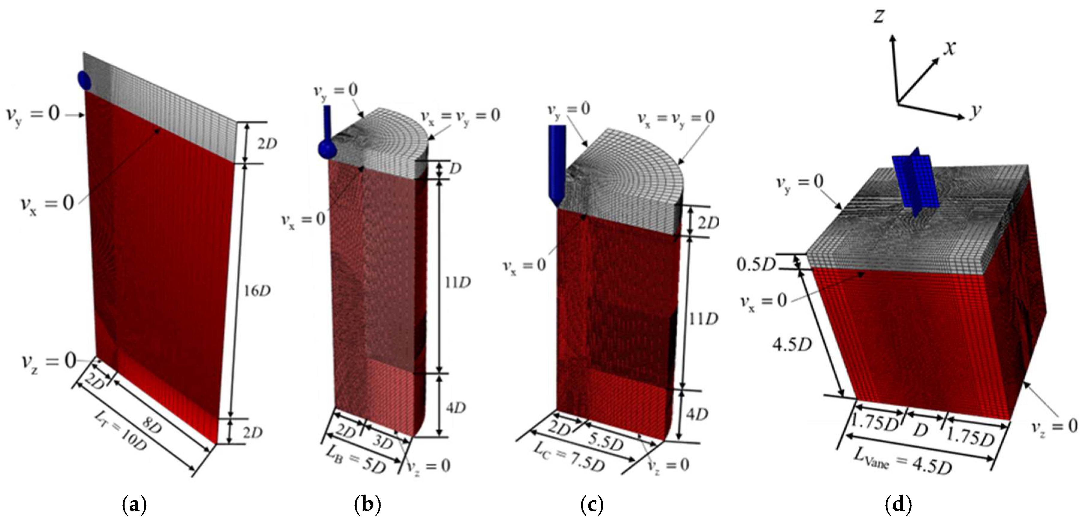
2.2. Geometry and FE Mesh

In this study, the CEL method was implemented using Abaqus/Explicit [44]. The soil region was modeled with eight-node reduced integration hexahedral elements (EC3D8R), and the various testing instruments were modeled using three-dimensional four-node rigid elements (R3D4). As shown in Figure 1, the Eulerian domain is divided into two parts: a clay material phase (colored red), assigned the mechanical properties of marine clay, and an initially unassigned void region (colored gray). The void region functions as a buffer zone to accommodate large soil displacements during penetrometer–soil interaction. The diameters of the ball penetrometer, cone penetrometer, T-bar penetrometer, and vane shear blade are denoted as D_Ball = 113 mm, D_Cone = 36 mm, D_T-bar = 40 mm, and D_Vane = 55 mm, respectively. Considering the slender, rod-like geometry of the T-bar penetrometer, this study adopts a plane strain assumption for its numerical modeling to reduce computational costs [45]. In the CEL method, since Eulerian domains only support three-dimensional hexahedral elements, the model of T-bar penetration was constructed as a single-layer mesh with a thickness set to D/20 as shown in Figure 1a [29,37]. The BPT (Figure 1b) and CPT (Figure 1c) models were modeled as one-quarter cylinders, and the VST (Figure 1d) is represented as a rectangular prism with dimensions of 4.5D × 4.5D × 4.5D. A high-resolution zone within 2D of the penetrometer captures strain localization, transitioning from D/20 to D/2 in peripheral regions. The contact interaction was controlled by the general contact algorithm, with normal behavior defined as hard contact to prevent interpenetration and tangential behavior modeled as frictionless. At the vane–soil interface, a tangential friction model based on the penalty method was selectively applied, with a Coulomb friction coefficient of 0.1 [31].

2.3. Constitutive Model and Material Parameters

To capture the strain-softening behavior and strain rate dependency inherent to soft clay, this study incorporates the modified Tresca constitutive model introduced by Einav and Randolph (2005) [39]. Although the model relies on accurate calibration of parameters such as μ, ${\xi }_{95}$, and ${\delta }_{\mathrm{rem}}$, the aim of this study is to compare the interpretation results of different testing methods under identical parameter conditions. Therefore, despite these limitations, the model remains effective in revealing the relative deviations and systematic errors among the various testing methods. The model expresses the undrained shear strength as a function of the maximum shear strain rate (${\dot{\gamma }}_{\max }$), with its formulation given as follows:

$$s_{\mathrm{u}}=\left[1+\mu \log \left({\displaystyle \frac{\max \left(\left|{\dot{\gamma }}_{\max }\right|,{\dot{\gamma }}_{\mathrm{ref}}\right)}{{\dot{\gamma }}_{\mathrm{ref}}}}\right)\right]\times \left[{\delta }_{\mathrm{rem}}+\left(1-{\delta }_{\mathrm{rem}}\right)e^{-3\xi /{\xi }_{95}}\right]s_{\mathrm{u}0}$$

(1)

where $\mu$ denotes the growth rate of shear strength per logarithmic cycle, typically ranging from 0.05 to 0.2 [46,47]. ${\dot{\gamma }}_{\max }$ is the maximum shear strain rate, calculated from $(△{\epsilon }_1-△{\epsilon }_3)/\Delta t$. ${\dot{\gamma }}_{\mathrm{ref}}$ represents the reference shear rate, typically taken as 1%/h [39], a value adopted in this study. Additionally, ${\delta }_{\mathrm{rem}}$ is the reciprocal of sensitivity $S_{\mathrm{t}}$, defined as the ratio of remolded strength to initial intact shear strength. $\xi$ represents the cumulative absolute maximum plastic shear strain, calculated from $\xi ={\displaystyle \int \left|{\dot{\gamma }}_{\max }\right|dt}$. ${\xi }_{95}$ is the cumulative shear strain required for 95% shear strength degradation, with typical values ranging from 10 to 50. $s_{\mathrm{u}0}$ denotes the initial intact shear strength at the reference shear strain rate ${\dot{\gamma }}_{\mathrm{ref}}$ before softening occurs. The model employs uniform strength properties with a constant Young’s modulus $E=300s_{\mathrm{u}}$, and the Poisson’s ratio is set to 0.495. The submerged unit weight of the soil is set to ${\gamma }^{\prime }=6.0{ \mathrm{kN}/\mathrm{m}}^3$ and the coefficient of horizontal earth pressure $K_0=1.0$. To elucidate method-specific discrepancies and interdependencies across in situ testing approaches, this study establishes a parametric study (detailed in

Table 1. Selected parameters for various testing methods in CEL analysis.

Testing Method	su0 (kPa)	μ	St	ξ95
TPT, BPT, CPT, VST	0.24, 1.0, 5.0, 10.0	-	-	-
TPT, BPT, CPT, VST	1.0	0.1	1.0	-
TPT, BPT, CPT, VST	1.0	0.1	10	10
TPT, BPT, CPT, VST	1.0	0	10	10, 30, 50

).

Since the modified Tresca model is not built in Abaqus, it must be implemented using the subroutine VUSDFLD. This subroutine enables the customization of material behavior and is well suited for incorporating complex constitutive models. The implementation approach follows a procedure similar to those adopted by Dutta et al. [48] and Han et al. [29]. A brief overview of the implementation process is provided below:

This process begins by retrieving the plastic strain tensor (${\epsilon }_{\mathrm{ij}}$) and stress tensor (${\sigma }_{\mathrm{ij}}$) at each integration point, updating them within each time increment, and storing the updated values in state variables. Next, parameters related to the modified Tresca model (e.g., $\mu$, ${\dot{\gamma }}_{\mathrm{ref}}$, ${\delta }_{\mathrm{rem}}$, ${\xi }_{95}$) were directly defined. During each time increment, both the absolute maximum shear strain rate $\left|{\dot{\gamma }}_{\max }\right|$ and the cumulative absolute maximum plastic shear strain $\xi$ were calculated. Then, $\left|{\dot{\gamma }}_{\max }\right|$ and ${\dot{\gamma }}_{\mathrm{ref}}$ were compared, and the maximum value was selected to prevent negative values in the logarithmic function during computation. Finally, $s_{\mathrm{u}}$ was assigned as a field variable to update the shear strength field at each time increment.

2.4. Loading Steps

In finite element analysis of various in situ tests, the process typically involves three analysis steps to simulate the penetration of different probes. Take the cone penetration test as an illustrative example:

(1)

Initial analysis step: As shown in Figure 1c, the velocity at the bottom boundary of the model was set to zero ($v_{\mathrm{z}}=0$), while the normal velocities at the two vertical face boundaries of the quarter-cylinder were also set to zero, corresponding to one vertical face as $v_{\mathrm{x}}=0$ and the other as $v_{\mathrm{y}}=0$. The velocity boundary for the cylindrical surface is defined as $v_{\mathrm{x}}=v_{\mathrm{y}}=0$. In this step, two predefined fields were established: one assigns the soil material to the Eulerian domain, and the other applies geostatic stress to the soil material portion.

(2)

Geostatic analysis step: A body force load was applied across the entire domain to simulate the influence of gravity. During this step, the displacement of the cone and push rod was constrained to prevent interaction with the soil. This constraint is implemented using a reference point, with a rigid body constraint established between the reference point and the conical rod. At the end of this step, the model shows only negligible deformation.

(3)

Penetration analysis step: A displacement load was applied to the reference point to drive the probe to the target depth. The displacement load is defined using a tabular amplitude curve to maintain a constant velocity during penetration.

In the vane shear test simulation, the first three steps adhere to the same procedural sequence. A fourth step, vane rotation analysis, was incorporated. During this step, a rotational load was applied and defined via a tabular amplitude curve to ensure a constant angular velocity throughout rotation.

2.5. Methodologies for Strength Interpretation

2.5.1. Vane Shear Test

During VST execution, a cruciform vane was inserted into the soil and rotated at a controlled angular velocity to measure the applied torque ($T$). This torque is typically divided into two components: the torque resisted by the horizontal surface ($T_{\mathrm{h}}$) and the cylindrical surface ($T_{\mathrm{v}}$). Wroth [5] proposed an expression assuming a shear stress distribution on the horizontal plane, given by

$${\displaystyle \frac{\tau }{{\tau }_{\mathrm{m}}}}={\left[{\displaystyle \frac{r}{D/2}}\right]}^n$$

(2)

where r represents the radial distance from the centerline on the horizontal surface, D is the diameter of the cylindrical failure surface, $\tau$ is the undrained shear stress at a distance r, ${\tau }_{\mathrm{m}}$ denotes the maximum shear stress occurring along the cylindrical surface, and $n$ is a coefficient dependent on the shear stress distribution shape on the horizontal surface. By integrating Equation (1), $T_{\mathrm{h}}$ can be calculated. Subsequently, under the assumption of isotropic soil strength, the torque is derived as

$$T=T_{\mathrm{h}}+T_{\mathrm{v}}={\displaystyle \frac{\pi D^3{\tau }_{\mathrm{m}}}{2(n+3)}}+{\displaystyle \frac{\pi D^{2}H{\tau }_{\mathrm{m}}}{2}}$$

(3)

where $H$ represents the vane height. For a typical vane with $H/D=2$, assuming uniform shear stress distribution on the horizontal surface (n = 0), the $s_{\mathrm{u}}$ is given by

$$\tau =s_{\mathrm{u}}={\displaystyle \frac{6T}{7\pi D^3}}$$

(4)

2.5.2. Cone Penetration Test

The estimation of $s_{\mathrm{u}}$ based on CPT results is typically expressed as [49]

$$s_{\mathrm{u}}={\displaystyle \frac{q_{\mathrm{net}}}{N_{\mathrm{kt}}}}={\displaystyle \frac{q-{\sigma }_v}{N_{\mathrm{kt}}}}$$

(5)

where $q_{\mathrm{net}}$ represents the net penetration resistance, $q$ denotes the cone resistance, $N_{\mathrm{kt}}$ is the cone resistance factor, and ${\sigma }_v$ stands for the total vertical overburden stress.

2.5.3. Ball and T-bar Penetration Test

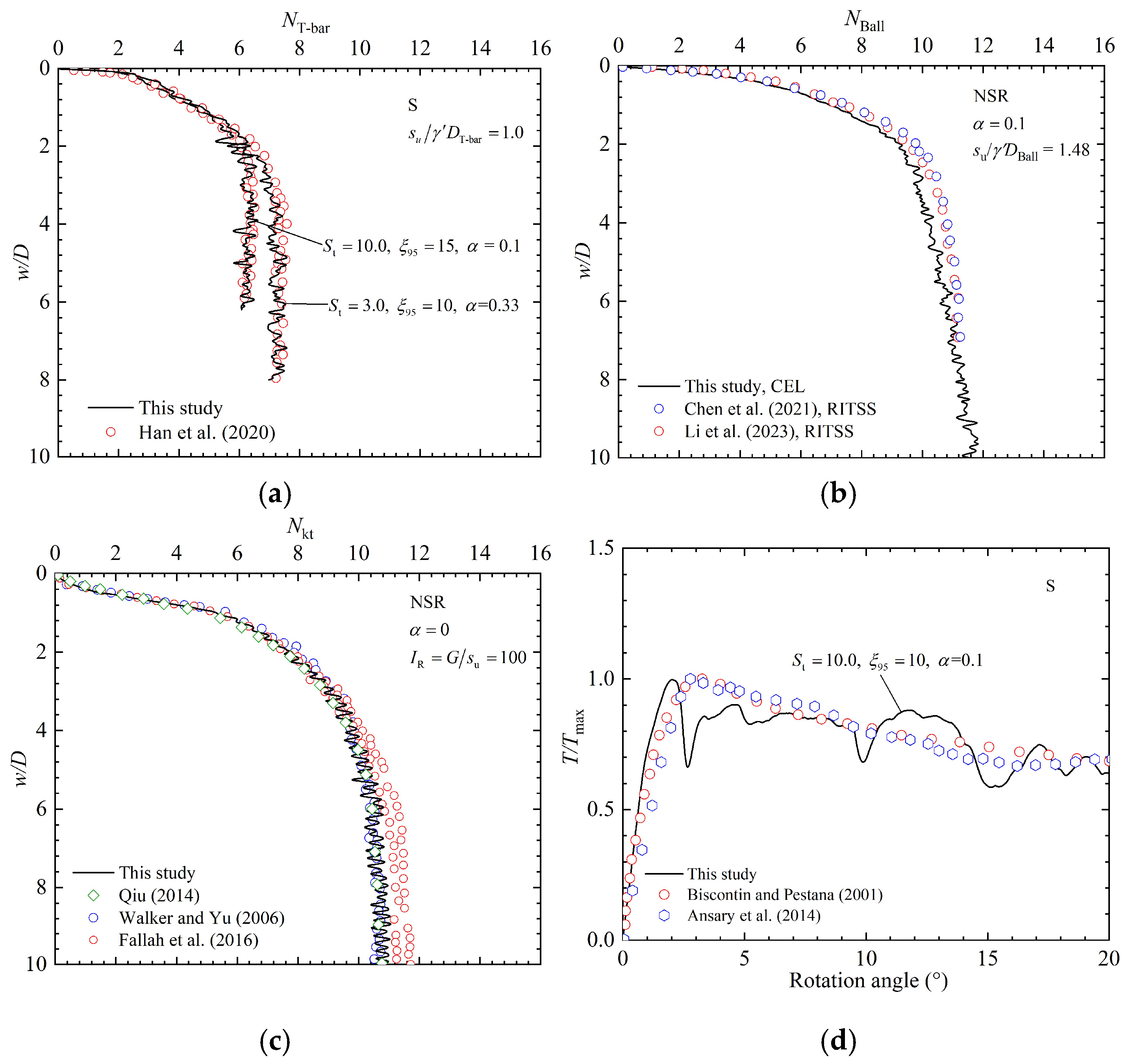
The net penetration resistance in T-bar penetration testing (TPT) and ball penetration testing (BPT) is determined by

$$q_{\mathrm{T}\text{-}\mathrm{bar}}=q_{\mathrm{Ball}}=q-\left[{\sigma }_v-u(1-a)\right]{\displaystyle \frac{A_{\mathrm{s}}}{A_{\mathrm{p}}}}$$

(6)

where $q_{\mathrm{T}\text{-}\mathrm{bar}}$ and $q_{\mathrm{Ball}}$ represent the net penetration resistance of the T-bar and the ball, respectively; u denotes the pore water pressure at the connection between the fully flowing probe and the push rod; a signifies the instrument’s unbalanced area ratio; and $A_{\mathrm{s}}$ and $A_{\mathrm{p}}$ represent the projected areas of the push rod and probe, respectively. The undrained shear strength is calculated from [50]

$$s_{\mathrm{u}}={\displaystyle \frac{q_{\mathrm{net}}}{N}}={\displaystyle \frac{q_{\mathrm{T}\text{-}\mathrm{bar}}}{N_{\mathrm{T}\text{-}\mathrm{bar}}}}={\displaystyle \frac{q_{\mathrm{Ball}}}{N_{\mathrm{Ball}}}}$$

(7)

where $N_{\mathrm{T}\text{-}\mathrm{bar}}$ represents the T-bar resistance factor, and $N_{\mathrm{Ball}}$ denotes the ball resistance factor.

3. Model Validation

A series of sensitivity analyses and a thorough verification process were conducted in this section. As shown in Figure 2, velocity sensitivity analyses were conducted for the BPT, VST, and CPT. The sensitivity analysis for TPT was not repeated here, as this study adopted the same modeling approach as Han et al. [29], who had already performed comprehensive validations. Their results demonstrated that, when the penetration velocity is set to D/10 s⁻¹, the influence of velocity on the penetration resistance becomes negligible. In addition, they showed that a mesh size of D/20 is sufficient to achieve mesh-independent results, as further refinement does not lead to significant changes in the computed resistance. For the BPT and CPT, $v$ in the figure represents the penetration velocity of the probe. As shown in Figure 2a, the verification results indicate that, at higher penetration rates, the penetration resistance factor may be overestimated. However, when the penetration velocity is D/10 s⁻¹, its effect on the resistance factor becomes negligible. Figure 2b shows the influence of penetration velocity on the cone resistance factor. This study adopts a penetration velocity of D/10 s⁻¹ to optimize computational accuracy and cost efficiency. Similarly, for the VST, $\omega$ represents the rotational speed of the vane. As shown in Figure 2c, when the rotation rate reaches 0.2° s⁻¹, the vane torque no longer decreases with a reduction in rotation speed, indicating that the effect of rotation speed on torque can be ignored.

Mesh sensitivity analyses, summarized in Figure 3a,b, reveal the convergence of resistance coefficients at a refined mesh size of D/20. Figure 3c shows that, when the mesh size of the VST model reaches D/25, the torque contributed by the vertical shear plane no longer decreases with further mesh refinement. This indicates that the influence of mesh size on the results becomes negligible at this point. Boundary effect validation, illustrated in Figure 4, confirms that the domain dimensions for BPT and CPT simulations sufficiently mitigate edge influences. For the VST model, boundary constraints adhere to the protocols established in Ansari et al.’s study [22].

Finally, mass scaling techniques were implemented to reconcile computational accuracy with efficiency. This method has been comprehensively validated by Kencana et al. [51]. As shown in Figure 5, increasing the model density by a factor of four yields computational results that are highly consistent before and after mass scaling, while reducing computation time by half. This validates the feasibility of the approach.

To validate the accuracy of the model, a comparison was conducted with the results of Tho et al. [37]. Figure 6a presents the soil deformation patterns obtained by Tho et al. [37] using the CEL method at different penetration depths for the T-bar. Correspondingly, Figure 6b shows the equivalent plastic strain contours from this study under the same material parameters. In the Eulerian framework, the equivalent plastic strain (PEEQVAVG) is calculated as a weighted average of the volume fractions of all materials within the element. This approach more accurately captures the overall plastic accumulation during material flow and quantifies the extent of the deformation. The results of this study closely align with those of Tho et al. [37], with regions of high equivalent plastic strain primarily concentrated along the path traversed by the T-bar during penetration.

Figure 7a presents T-bar penetration test results for two cohesive soils with distinct sensitivity levels. The high-sensitivity soil exhibits a markedly lower resistance factor, corroborating the experimental findings of Han et al. [29]. In this study, “S” represents only the softening effect, “R” represents only the rate effect, “SR” represents both the softening and rate effects, and “NSR” represents the scenario where neither effect is considered. Additionally, $\alpha$ denotes the roughness factor. Figure 7b presents the depth-dependent $N_{\mathrm{Ball}}$ curve obtained by Chen et al. [52] and Li et al. [53] using the RITSS method, which was successfully reproduced in this study using the CEL method. In the initial penetration phase, the results of this study exhibit excellent agreement with those of previous studies. However, as the penetration depth increases, the ball enters the trapped cavity phase, causing interaction between the push rod and the soil, which leads to a continuous increase in penetration resistance with depth. Therefore, this effect requires further correction. Figure 7c,d show the simulation results for CPT and VST, respectively, both of which exhibit strong consistency with existing studies [22,47,54,55,56]. These findings confirm the high accuracy of the developed numerical model.

4. Results and Discussion

4.1. Shear Failure Process Analysis

In the VST, the vane is slowly driven into the soil until reaching the predetermined depth, after which controlled torsional loading is applied. Figure 8 illustrates the equivalent plastic strain distribution at the middle section of the vane’s cross-section as the torsional angle increases in the model. At the end of penetration, localized plastic strains develop near the vane–soil interface, while pronounced strain concentrations emerge at the central area. Under subsequent torsion, a square-shaped plastic zone initially forms around the vane. As torsional displacement progresses, this zone transitions into a radially circular pattern, indicative of shear band development and strain redistribution.

Compared with the vane shear test, the ball and T-Bar penetrometers exhibit three distinct penetration phases due to their axisymmetric geometries and continuous soil-probe interaction (as shown in Figure 9 and Figure 10): (1) open cavity state, (2) trapped cavity state, and (3) full-flow state. In the Figure 9 and Figure 10, $w_{\mathrm{c}}$ represents the critical depth from the open cavity phase to the cavity-trapped phase, while $w_{\mathrm{d}}$ denotes the critical depth from the cavity-trapped phase to the full-flow phase. In the initial open cavity state, the penetration resistance increases rapidly. When the penetration depth reaches approximately 4.8D, the ball enters the cavity-trapped phase. As penetration depth increases, the failure mechanism of the probe gradually transitions progressively from the trapped cavity mechanism to the full-flow mechanism, accompanied by a slight increase in the resistance factor. The ball enters the full-flow phase only when the penetration depth reaches around 7.5D, at which point the resistance factor stabilizes and remains constant. The shear failure mechanism of the TPT is consistent with that of the BPT. However, the critical depths for transitioning between different failure mechanisms differ, being approximately 10.6D and 20.4D, respectively.

Figure 11 presents the cone resistance factor variation with depth and deformation characteristics at different stages. During the initial stage of the cone penetration test (penetration depth of D), the cone penetrometer fully contacts the soil. As the cone tip advances through the soil, significant equivalent plastic strain develops in the cone tip region. Compared to the T-bar and ball penetrometers, the cone penetrometer is enveloped by the soil more rapidly. As penetration depth increases, the equivalent plastic strain around the cone penetrometer gradually rises, with the maximum equivalent plastic strain occurring at the slanted surface. When the penetration depth reaches 8D, the resistance factor stabilizes and no longer changes.

Figure 12 depicts the evolution of shear failure mechanisms for each testing penetrometer at penetration depths of 2D, 5D, and 10D. The left panel displays the distribution of equivalent plastic strain, while the right panel illustrates the flow vectors of the clay during penetration. The red arrows indicate the flow direction of the soil material during probe–soil interaction in the testing process. Figure 12a,b demonstrates that the ball and T-bar probes induce significant soil deformation during penetration, with peak equivalent plastic strain concentrated at their tips. Velocity vector diagrams further illustrate pronounced soil backflow during both probe operations. Compared to the BPT and TPT, the CPT induces larger equivalent plastic strain near the probe (Figure 12c), but with a smaller affected zone. Additionally, cone penetration velocity vectors visually demonstrate lateral soil displacement caused by the advancing cone tip.

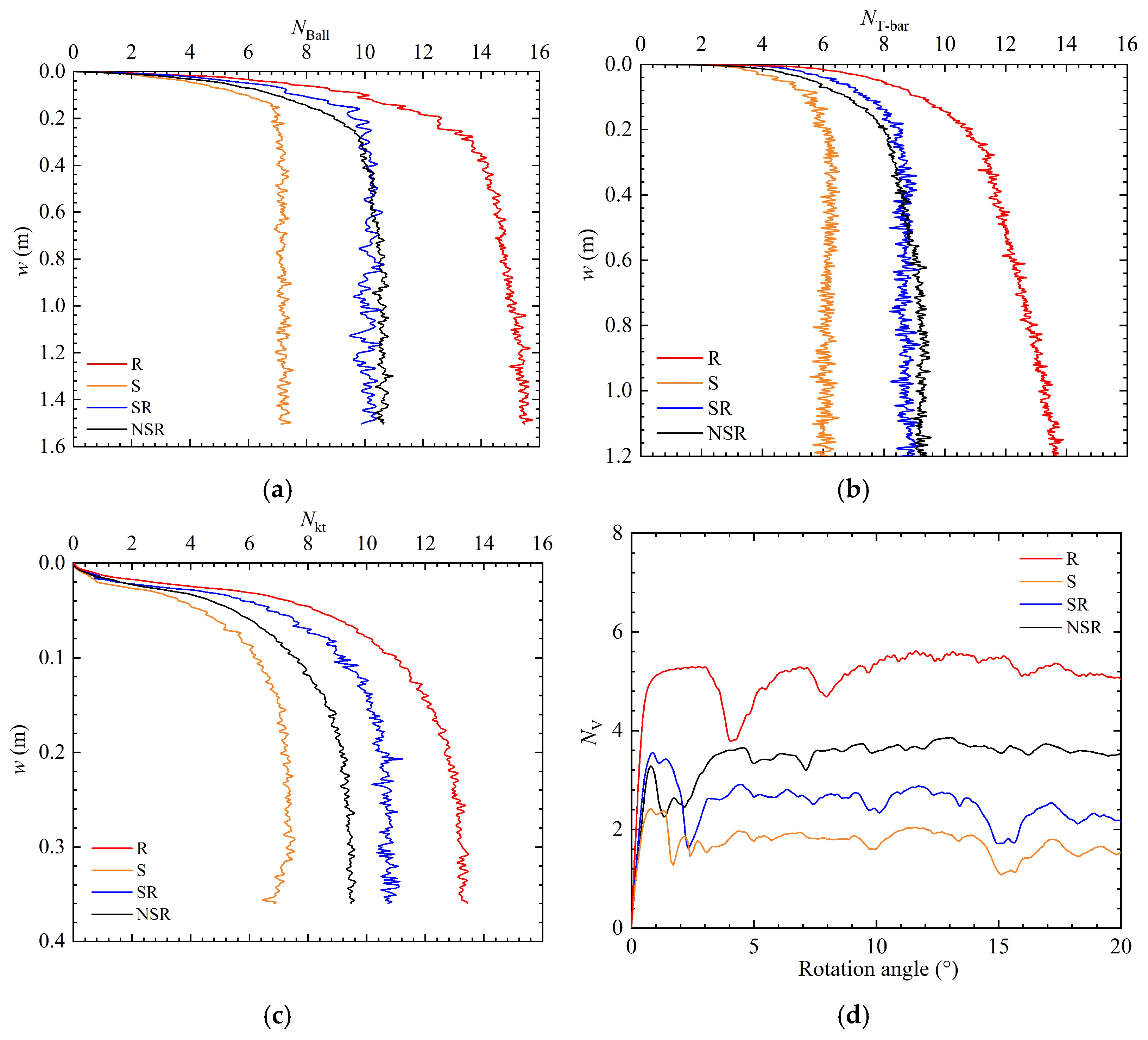
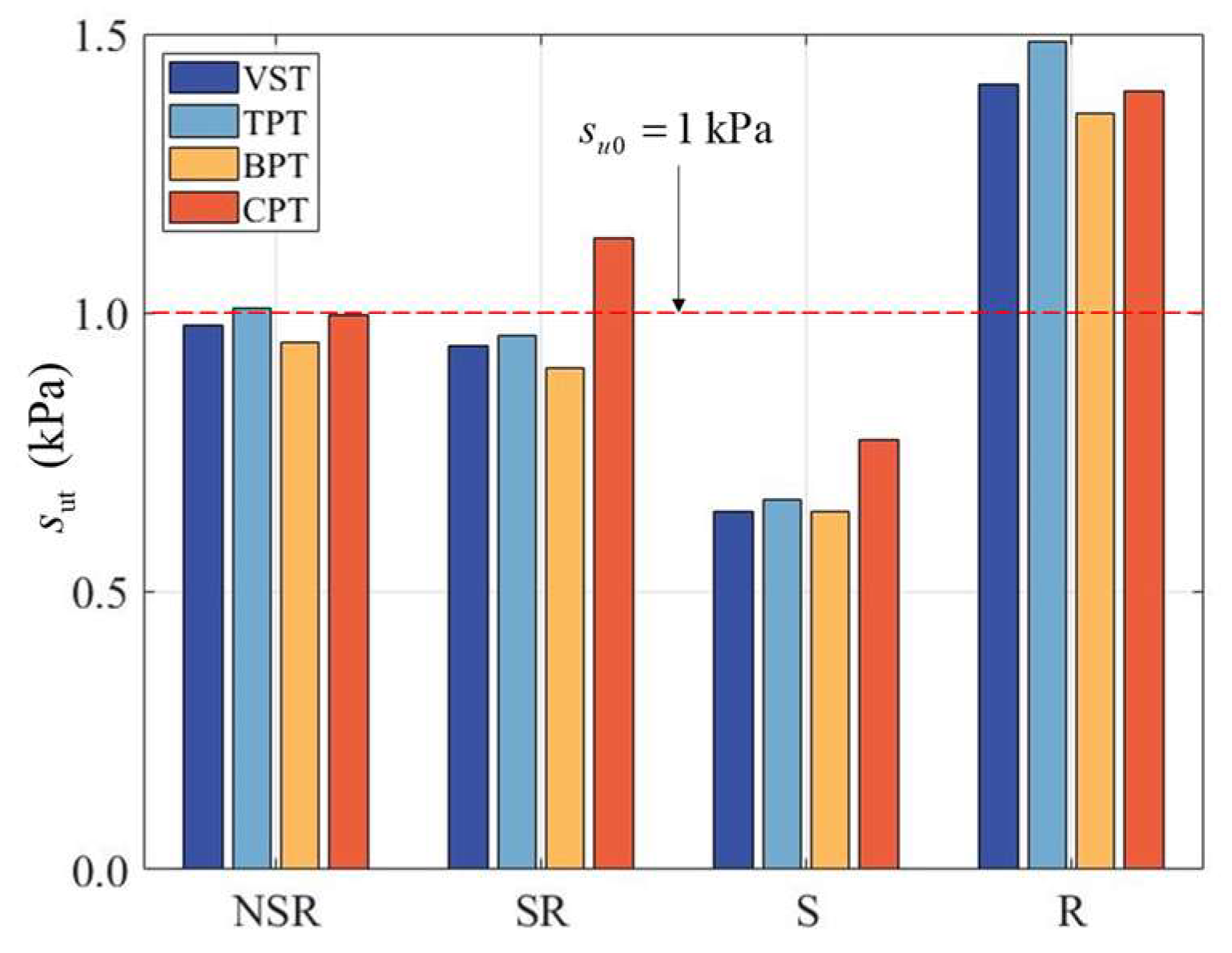
4.2. Comparative Analyses of Various Testing Methods

This study performed multiple strength test series to investigate the adaptability of four testing methods in cohesive soils across varying strength ranges. As shown in Figure 13a,b, ball (BPT) and T-bar (TPT) penetration tests at 10D penetration depth reveal that high-strength ($s_{\mathrm{u}0}=5.0 \mathrm{kPa}$, $s_{\mathrm{u}0}=10.0 \mathrm{kPa}$) cohesive soils exhibit limited plastic deformation, inhibiting full-flow mechanism development. Consequently, the resistance factor, calculated as the ratio of net penetration resistance to initial shear strength, significantly deviates from the theoretical value. The resistance factor ($N$) is computed using

$$N={\displaystyle \frac{q_{\mathrm{net}}}{s_{\mathrm{u}0}}}$$

(8)

For low-strength ($s_{\mathrm{u}0}=0.24 \mathrm{kPa}$) soils, the resistance factor calculated using Equation (8) may be overestimated. Tho et al. [37] corrected the net penetration resistance by accounting for the self-weight of the soil uplift, bringing the resistance factor closer to the theoretical value. In the case where the soil strength is 1.0 kPa, as the penetration depth increases, both the ball and T-bar enter the full-flow phase. The T-bar resistance factor $N_{\mathrm{T}\text{-}\mathrm{bar}}$ converges closely with the theoretical value of 9.14 proposed by Martin and Randolph. [57]. It is noteworthy that the resistance factor of the ball is slightly lower than the average theoretical value of 11.20 from existing studies (under smooth conditions, the lower-bound solution is 10.98, and the upper-bound solution is 11.80 in Randolph et al. [58], while a smaller upper-bound solution of 11.36 was obtained in Einav and Randolph [39]). This discrepancy occurs because theoretical calculations neglect the influence of the rod itself, an explanation validated by Zhou et al. [24]. Similar findings have also been reported in Gu et al. [26]. In a study of CPTs, Gu et al. [59] combined the CEL method with laboratory model tests, proposing a recommended value of 9.50 for the cone penetrometer’s resistance factor. The numerical study by Walker and Yu [54] established a correlation between the cone factor $N_{\mathrm{kt}}$ and the rigidity index ($I_{\mathrm{R}}=G/s_{\mathrm{u}}$) under smooth conditions, expressed as

$$N_{\mathrm{kt}}=2.0167\ln (G/s_u)+0.2092$$

(9)

In this study, with the $I_{\mathrm{R}}$ set to 100, the same $N_{\mathrm{kt}}$ was calculated. As shown in Figure 13c, when the cone penetration factor stabilizes with depth, the resistance factor obtained in this study aligns with their results. Additionally, it was observed that the cone resistance factor remains largely unchanged under different strength conditions. To facilitate comparison across multiple testing methods, this study defines a vane resistance factor $N_{\mathrm{V}}$, representing dimensionless torque, with the specific expression given by

$$N_{\mathrm{V}}={\displaystyle \frac{T}{s_{\mathrm{u}}{D}^3}}$$

(10)

From Equations (4) and (10), $N_{\mathrm{V}}=3.66$ can be calculated. Figure 13d illustrates the variation in the resistance factor under different strength conditions, indicating that $N_{\mathrm{V}}$ is less sensitive to changes in strength.

Figure 13. Variation in results of the four testing methods under different strength conditions: (a) $N_{\mathrm{Ball}}$ [39,58]; (b) $N_{\mathrm{T}\text{-}\mathrm{bar}}$ [57]; (c) $N_{\mathrm{kt}}$ [54,59]; and (d) $N_{\mathrm{V}}$.

Figure 13. Variation in results of the four testing methods under different strength conditions: (a) $N_{\mathrm{Ball}}$ [39,58]; (b) $N_{\mathrm{T}\text{-}\mathrm{bar}}$ [57]; (c) $N_{\mathrm{kt}}$ [54,59]; and (d) $N_{\mathrm{V}}$.

To analyze the differences in strength interpretation values obtained from various testing methods, this study first derives penetration resistance ($q$) and torque ($T$) through numerical simulations. The strength interpretation values ($s_{\mathrm{ut}}$) for the four testing methods are calculated using Equations (4)–(7). In this study, the influence of pore water pressure is neglected, and the TPT model is simulated without a rod, leading to the derivation of the following equations:

$$q_{\mathrm{T}\text{-}\mathrm{bar}}=q$$

(11)

$$q_{\mathrm{Ball}}=q-{\sigma }_v{\displaystyle \frac{A_{\mathrm{s}}}{A_{\mathrm{p}}}}$$

(12)

For penetration tests (TPT, BPT, CPT), empirical relationships based on measured data from different regions are typically established in engineering practice to determine shear strength, with the resistance factor often as an empirical value. In this study, theoretical values of the resistance factor from related research are selected to calculate $s_{\mathrm{ut}}$. For the T-bar and ball, the previously mentioned theoretical values of 9.14 and 11.20 are used for the resistance factor. For the selection of the cone resistance factor, based on Walker and Yu [54] and Gu et al. [59], a value of $N_{\mathrm{kt}}=9.50$ was selected.

Following the interpretation of multiple experimental datasets, as shown in Figure 14, the ball (BPT) and T-bar (TPT) penetrometers in high-strength soils fail to fully mobilize the full-flow mechanism. Under this cavity-trapped mechanism, the measurement of $s_{\mathrm{u}0}$ is underestimated, with the strength interpretation value $s_{\mathrm{ut}}$ deviating by up to 15% from the initial undrained shear strength $s_{\mathrm{u}0}$. Therefore, it is advisable to avoid using these two testing methods for soils with high undrained shear strength. For the CPT and VST, the results indicate that the ratio of interpreted shear strength to initial shear strength is essentially consistent, meaning that the interpreted results are relatively unaffected by the initial shear strength. Since the selected cone resistance factor closely matches the factor derived from interpretation, the standardized interpreted shear strength value for the CPT is approximately 1. However, the VST interpretation underestimates the initial drained shear strength by about 5.7%, suggesting that the vane shear strength interpretation is conservative. This discrepancy is likely due to the non-uniform distribution of shear stress on the vane blades during torsion, which differs from the conventional assumption of uniform distribution. These findings highlight the systematic errors present in various testing methods during testing.

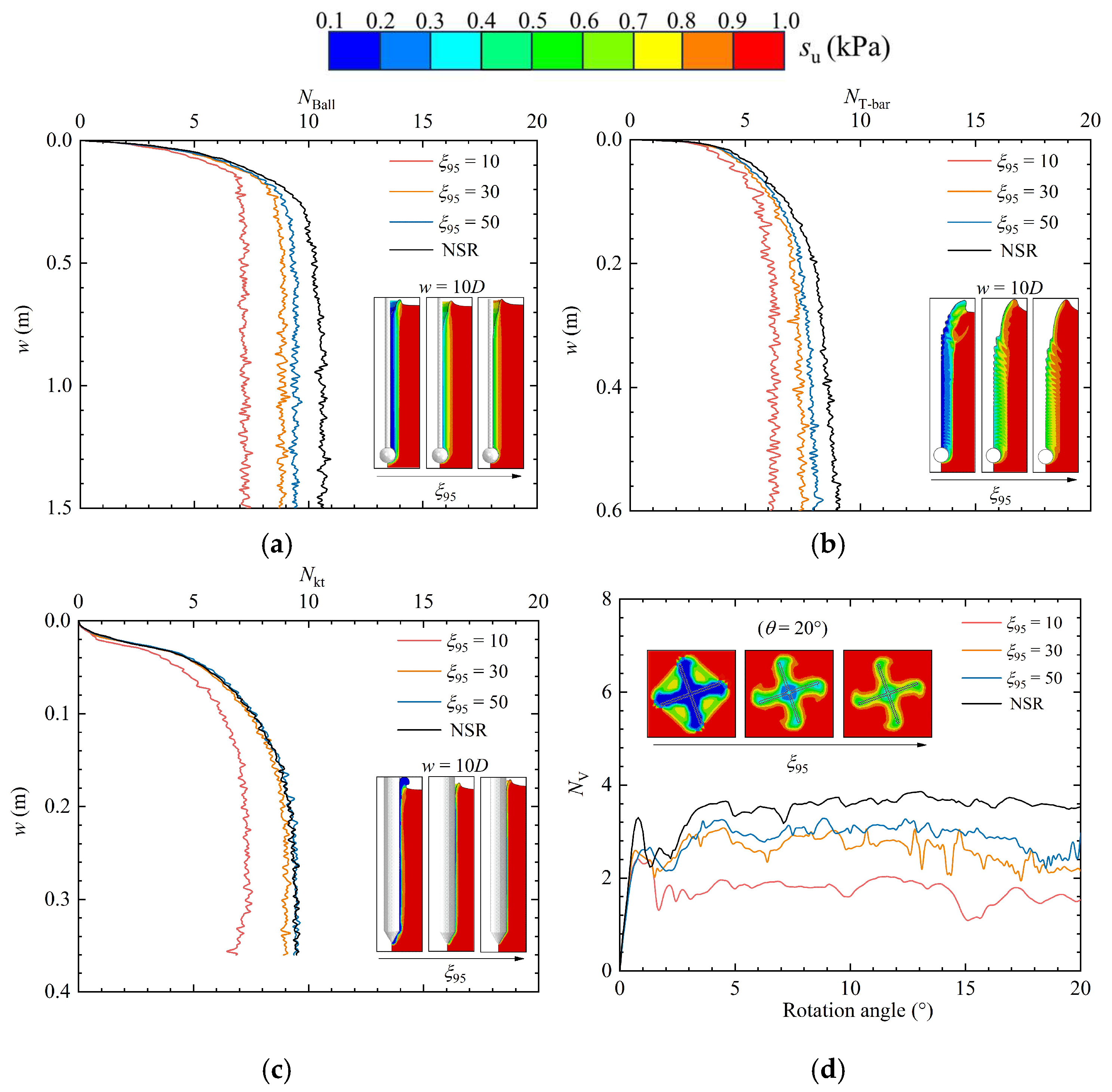
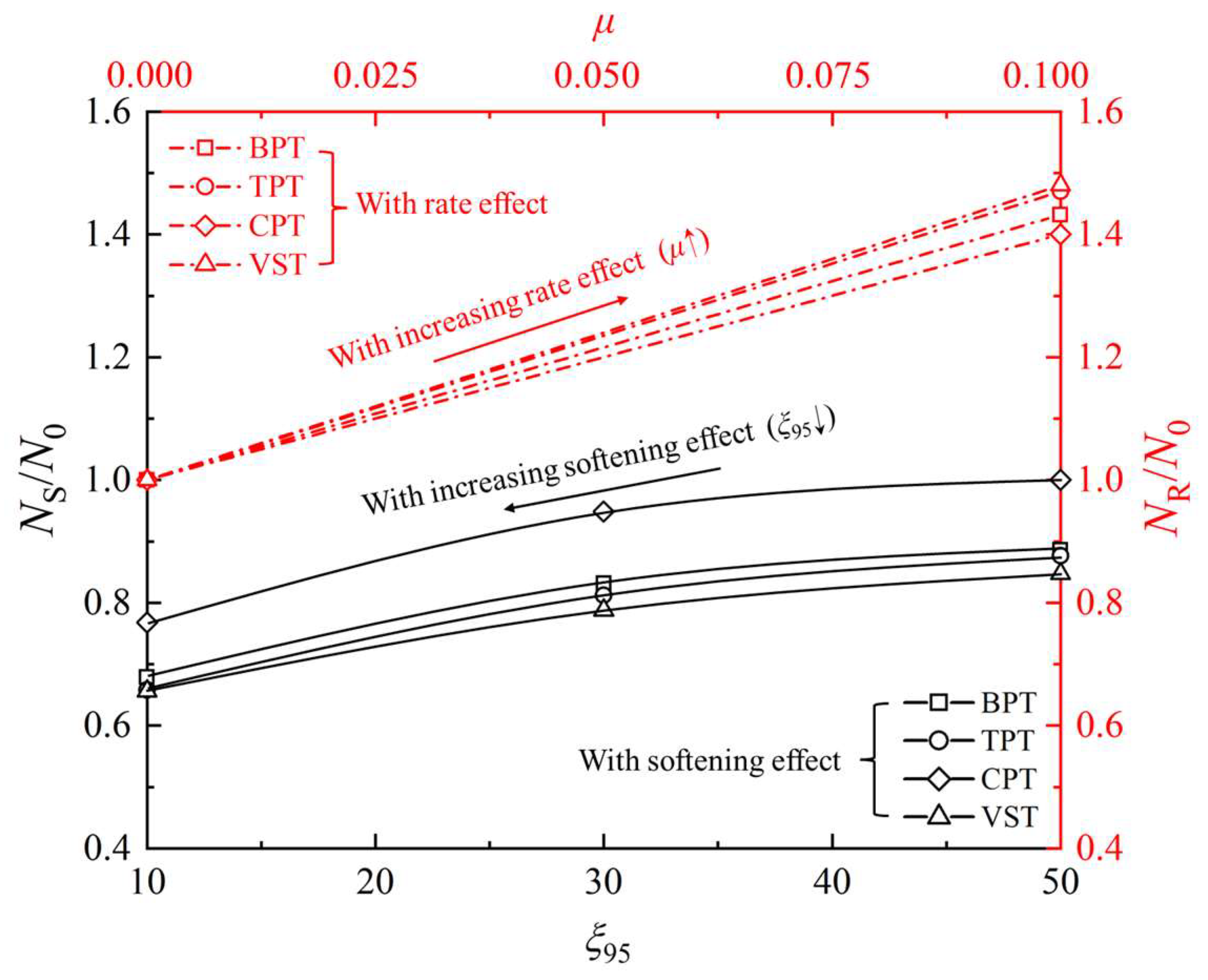
4.3. Analysis of the Softening Effect and Rate Effect Results

To comparatively analyze strain softening and strain rate effects on the four testing methodologies, this study conducted simulations under various combinations of softening and rate effects. Figure 15 illustrates the variations in resistance factors across the four testing methods under different effect considerations. In this section, four working conditions are examined: (1) considering only the rate effect ($\mu =0.1, S_{\mathrm{t}}=1$); (2) considering only the softening effect ($\mu =0, S_{\mathrm{t}}=10, {\xi }_{95}=10$); (3) considering neither effect ($\mu =0, S_{\mathrm{t}}=1$); and (4) considering both effects ($\mu =0.1, S_{\mathrm{t}}=10, {\xi }_{95}=10$). By comparing the NSR and S curves, it can be seen that, after considering the softening effect, the resistance factors from all strength testing methods decrease. A further comparison between Figure 16a,b shows that the softening effect reduces the local shear strength around the ball. On the other hand, the comparison between the NSR and R curves indicates that, after considering the rate effect, the resistance factors measured by various strength testing methods increase. As shown in Figure 16a,c, the rate effect enhances the local shear strength around the ball. Therefore, when both effects are considered simultaneously, their competitive mechanism governs the soil deformation: softening-induced strength degradation counteracts rate-induced strengthening. Figure 16d shows the shear strength field distribution during BPT penetration. In region A₁, where the cumulative plastic strain is significant, the softening effect is more pronounced, reducing shear strength. In region A₂, where cumulative plastic strain is minimal, the rate effect dominates, increasing shear strength.

By comparing the SR and NSR curves in Figure 15, it can be found that, before and after considering both rate and softening effects, factors from the BPT, TPT, and VST show a slight decrease, as the strain softening effect outweighs the local strain rate hardening effect. In contrast, CPT simulations show that strain-rate hardening dominates, with the increase in localized shear strength exceeding softening-induced degradation, resulting in a 13.5% elevation in penetration resistance relative to NSR models.

Following the interpretation of resistance and torque data obtained from the four testing methodologies, the undrained shear strength values $s_{\mathrm{ut}}$ interpreted from the CPT, TPT, BPT, and VST exhibit significant method-dependent variations under the modified Tresca constitutive framework, governed by competing strain-rate hardening and strain-softening mechanisms, as shown in Figure 17. When only the rate effect is considered, the undrained shear strength increases by 40–50% across all methods. Conversely, when only the softening effect is considered, the undrained shear strength decreases by 23–35% in all tests. In the CPT, the strain softening effect exhibits a comparatively weaker influence on resistance reduction than that observed in other testing methods, indicating that strain-rate hardening dominates. Under isolated rate effect conditions, the resistance increase observed in CPT is comparable to that observed in other methods. Consequently, when both rate and softening effects are concurrently modeled, the CPT-derived $s_{\mathrm{ut}}$ values are markedly higher than those from the TPT, BPT, and VST.

In light of the methodological inconsistencies previously noted in strain-softening responses, a focused investigation of the softening parameter ξ₉₅ was undertaken. Figure 18 illustrates the variation in resistance factors under different ξ₉₅. The cloud plot in the lower-right corner of the figure shows the shear strength field distribution at a penetration depth of 10D for different ξ₉₅ values (from left to right: ξ₉₅ = 10, 30, 50). As shown in Figure 18a, as ξ₉₅ increases, less soil enters the fully remolded state (s_u0 = 0.1 kPa), leading to higher resistance factor values.

Figure 19 compares the performance of different testing methods under the isolated examination of rate effects and softening effects. Here, $N_{\mathrm{S}}$ represents the resistance factor when only the softening effect is considered, while $N_{\mathrm{R}}$ denotes the factor considering only rate effects. The resistance factor $N_0$ is defined under conditions excluding both rate dependency and the softening behavior. $N_{\mathrm{S}}/N_0$ represents the factor reduction ratio, indicating the extent of change in the factors of each testing method after considering softening. $N_{\mathrm{R}}/N_0$ represents the factor amplification ratio. Figure 19 reveals that the resistance factors obtained from the four testing methods exhibit distinct growth rates with increasing $\mu$ values, following the order CPT < BPT < TPT < VST. Similarly, as the parameter ${\xi }_{95}$ decreases, the resistance factors decline with varying magnitudes across methods, following the sequence: CPT, BPT, TPT, and VST from the smallest to the largest reduction. Notably, when considering only the softening effect, the CPT achieves significantly higher penetration resistance than the TPT, BPT, and VST, due to its relatively lower sensitivity to softening.

5. Conclusions

This study investigates the relationships between different in situ testing methods for the undrained shear strength of soft clay. Using the CEL method, we developed finite element models of four strength testing methods and performed a comprehensive comparative analysis of their interpreted values. The key findings are summarized as follows:

(1)

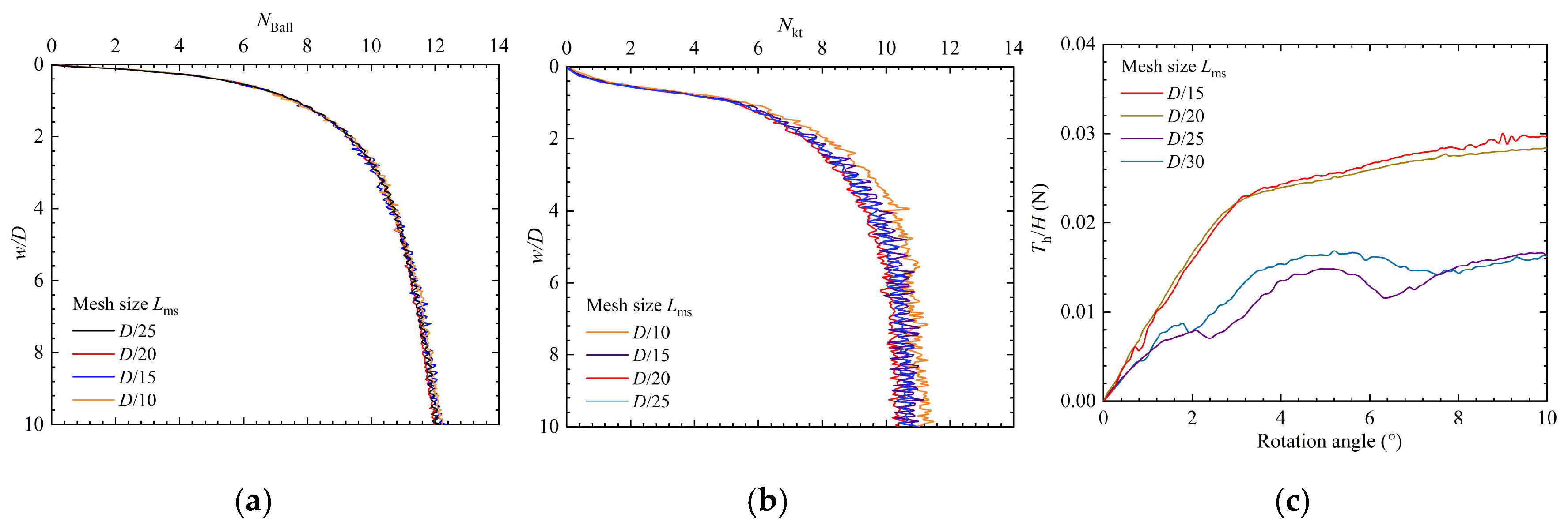
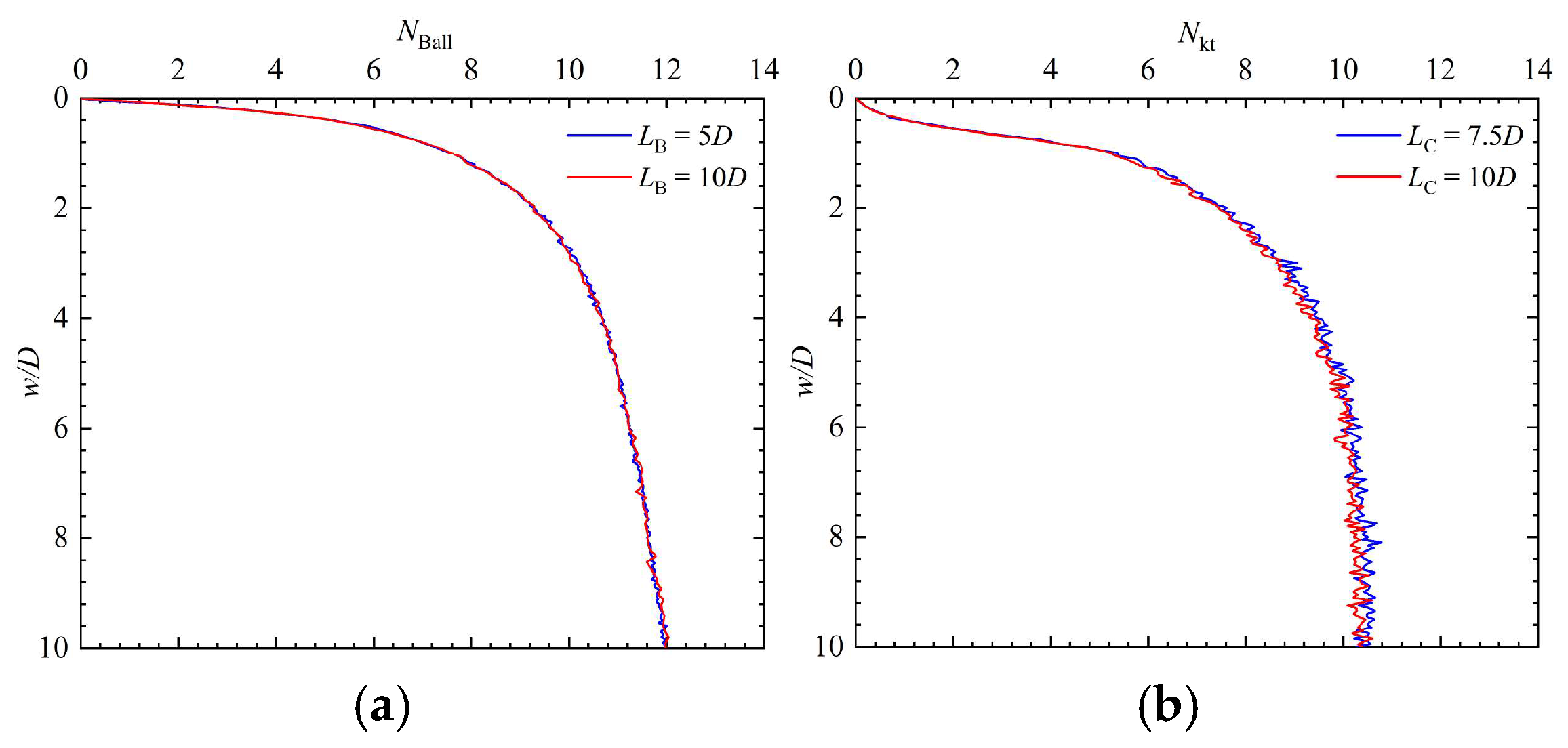
Model Validation: A systematic evaluation of the FE models for multiple in situ testing methods is performed, focusing on velocity sensitivity, mesh sensitivity, boundary effects, and mass scaling. The results consistently validated the reliability of the simulation framework.

(2)

Failure Mechanism Analysis: The CEL method effectively captured distinct failure patterns across different testing methods. In the VST simulation, progressive shear failure of the soil surrounding the vane was observed, accompanied by a geometric transition of the failure surface from square to circular with an increasing torsion angle. Both BPT and TPT simulations demonstrated the characteristic three-phase penetration behavior: cavity initiation, cavity confinement, and full-flow development. The CPT simulation revealed soil displacement around the cone tip, with maximum equivalent plastic strain concentrated along the conical interface.

(3)

Interpreted Strength Variations: When neglecting strain softening and rate effects, the interpreted strength values ($s_{\mathrm{ut}}$) showed method-dependent variations due to differing shear failure mechanisms. While the VST and CPT exhibited minimal deviation in the ratio of the interpreted values to the initial shear strength, the BPT and TPT underestimated strength by approximately 15% in high-strength soils where full-flow mechanisms failed to develop completely.

(4)

Constitutive Effects: The combined consideration of softening and rate effects produced contrasting results across methods. The TPT, BPT, and VST showed slight decreases (4–5%) in interpreted strength, while CPT values increased by 13.5%. This discrepancy stems from the CPT’s reduced sensitivity to cumulative plastic strain effects. When only the softening effect is considered, strain softening had significantly less impact on the CPT ($N_{\mathrm{S}}/N_0$≈0.76–1.00) compared to other methods ($N_{\mathrm{S}}/N_0$≈0.65–0.88) under identical ${\xi }_{95}$ conditions.

These findings contribute to a deeper understanding of the intrinsic differences and interrelations among the interpreted results from various in situ strength testing methods. In previous studies, strength interpretation frameworks were typically developed independently for each testing method, often using different numerical approaches, which introduced unavoidable discrepancies in cross-method comparisons. By employing a consistent modeling framework to simulate four widely used test types, this study systematically analyzed the origins of interpretation differences, examined each method’s applicability under varying strength conditions, and quantified the effects of key constitutive behaviors. The outcomes offer a new perspective on undrained strength interpretation and serve as a valuable reference for future efforts aimed at establishing consistent correlations among different in situ test results.

References

1. Randolph, M.F.; Gaudin, C.; Gourvenec, S.M.; White, D.J.; Boylan, N.; Cassidy, M.J. Recent advances in offshore geotechnics for deep water oil and gas developments. Ocean Eng. 2011, 38, 818–834. [Google Scholar] [CrossRef]
2. Wang, Y.; Cassidy, M.J.; Bienen, B. Numerical investigation of bearing capacity of spudcan foundations in clay overlying sand under combined loading. J. Geotech. Geoenviron. Eng. 2020, 146, 04020117. [Google Scholar] [CrossRef]
3. Wang, N.; Qi, W.G.; Gao, F.P. Predicting the instability trajectory of an obliquely loaded pipeline on a clayey seabed. J. Mar. Sci. Eng. 2022, 10, 299. [Google Scholar] [CrossRef]
4. Stefanow, D.; Dudziński, P.A. Soil shear strength determination methods–State of the art. Soil Tillage Res. 2021, 208, 104881. [Google Scholar] [CrossRef]
5. Wroth, C.P. The interpretation of in situ soil tests. Géotechnique 1984, 34, 449–489. [Google Scholar] [CrossRef]
6. Low, H.E.; Randolph, M.F. Strength measurement for near-seabed surface soft soil using manually operated miniature full-flow penetrometer. J. Geotech. Geoenviron. Eng. 2010, 136, 1565–1573. [Google Scholar] [CrossRef]
7. Ma, H.; Zhou, M.; Hu, Y.; Hossain, M.S. Effects of cone tip roughness, in-situ stress anisotropy and strength inhomogeneity on CPT data interpretation in layered marine clays: Numerical study. Eng. Geol. 2017, 227, 12–22. [Google Scholar] [CrossRef]
8. Chung, S.G.; Kim, G.J.; Kim, M.S.; Ryu, C.K. Undrained shear strength from field vane test on busan clay. Mar. Georesour. Geotec. 2007, 25, 167–179. [Google Scholar] [CrossRef]
9. Chandler, R.J. The in-situ measurement of the undrained shear strength of clays using the field vane. In Vane Shear Strength Testing in Soils: Field and Laboratory Studies; Richards, A.F., Ed.; ASTM: West Conshohocken, PA, USA, 1988; Volume 1014, pp. 13–44. [Google Scholar]
10. Robertson, P.K.; Cabal, K. Guide to Cone Penetration Testing, 7th ed.; Gregg Drilling LLC: Signal Hill, CA, USA, 2022. [Google Scholar]
11. Qi, W.G.; Gao, F.P.; Randolph, M.F.; Lehane, B.M. Scour effects on p–y curves for shallowly embedded piles in sand. Géotechnique 2016, 66, 648–660. [Google Scholar] [CrossRef]
12. Li, B.; Qi, W.-G.; Wang, Y.; Gao, F.-P.; Wang, S.-Y. Scour-induced unloading effects on lateral response of large–diameter monopiles in dense sand. Comput. Geotech. 2024, 174, 106635. [Google Scholar]
13. Fu, S.; Shen, Y.; Jia, X.; Zhang, Z. A novel method for estimating the undrained shear strength of marine soil based on CPTU tests. J. Mar. Sci. Eng. 2024, 12, 1019. [Google Scholar] [CrossRef]
14. Lunne, T.; Randolph, M.F.; Chung, S.F.; Andersen, K.H.; Sjursen, M. Comparison of cone and t-bar factors in two onshore and one offshore clay sediments. In Proceedings of the International Symposium on Frontiers in Offshore Geotechnics, Perth, Australia, 1 January 2005; pp. 981–989. [Google Scholar]
15. Lunne, T.; Andersen, K.H.; Low, H.E.; Randolph, M.F.; Sjursen, M. Guidelines for offshore in situ testing and interpretation in deepwater soft clays. Can. Geotech. J. 2011, 48, 543–556. [Google Scholar] [CrossRef]
16. Randolph, M.F.; Hefer, P.A.; Geise, J.M.; Watson, P.G. Improved seabed strength profiling using T-bar penetrometer. In Proceedings of the International Conference on Offshore Site Investigation and Foundation Behaviour: New Frontiers, London, UK, 22–24 September 1998; pp. 221–235. [Google Scholar]
17. Stewart, D.P.; Randolph, M.F. T-bar penetration testing in soft clay. J. Geotech. Eng. 1994, 120, 2230–2235. [Google Scholar] [CrossRef]
18. Kelleher, P.J.; Randolph, M.F. Seabed geotechnical characterization with the portable remotely operated drill. In Proceedings of the International Symposium on Frontiers in Offshore Geotechnics, Perth, Australia, 19–21 September 2005; pp. 365–371. [Google Scholar]
19. DeJong, J.; Yafrate, N.; DeGroot, D.; Low, H.E.; Randolph, M. Recommended practice for full-flow penetrometer testing and analysis. Geotech. Test. J. 2010, 33, 137–149. [Google Scholar] [CrossRef]
20. Liyanapathirana, D.S. Arbitrary Lagrangian Eulerian based finite element analysis of cone penetration in soft clay. Comput. Geotech. 2009, 36, 851–860. [Google Scholar] [CrossRef]
21. Zhang, W.; Zou, J.; Zhang, X.; Yuan, W.; Wu, W. Interpretation of cone penetration test in clay with smoothed particle finite element method. Acta Geotech. 2021, 16, 2593–2607. [Google Scholar] [CrossRef]
22. Ansari, Y.; Pineda, J.; Kouretzis, G.; Sheng, D. Experimental and numerical investigation of rate and softening effects on the undrained shear strength of Ballina clay. Aust. Geomech. J. 2014, 49, 51–58. [Google Scholar]
23. White, D.J.; Gaudin, C.; Boylan, N.; Zhou, H. Interpretation of t-bar penetrometer tests at shallow embedment and in very soft soils. Can. Geotech. J. 2010, 47, 218–229. [Google Scholar] [CrossRef]
24. Zhou, M.; Hossain, M.S.; Hu, Y.; Liu, H. Behaviour of ball penetrometer in uniform single-and double-layer clays. Géotechnique 2013, 63, 682–694. [Google Scholar] [CrossRef]
25. Wang, Y.; Hu, Y.; Hossain, M.S.; Zhou, M. Effect of trapped cavity mechanism on interpretation of T-Bar penetrometer data in uniform clay. J. Geotech. Geoenviron. Eng. 2020, 146, 04020078. [Google Scholar] [CrossRef]
26. Gu, Z.; Guo, X.; Nian, T.; Fu, C.; Zhao, W. An improved evaluation method for the undrained shear strength of uniform soft clay in the nonfull flow state based on ball penetration simulations. Appl. Ocean Res. 2022, 128, 103365. [Google Scholar] [CrossRef]
27. Randolph, M.F.; Andersen, K.H. Numerical analysis of T-bar penetration in soft clay. Int. J. Geomech. 2006, 6, 411–420. [Google Scholar] [CrossRef]
28. Shen, J.; Wang, X.; Chen, Q.; Ye, Z.; Gao, Q.; Chen, J. Numerical investigations of undrained shear strength of sensitive clay using miniature vane shear tests. J. Mar. Sci. Eng. 2023, 11, 1094. [Google Scholar] [CrossRef]
29. Han, Y.; Yu, L.; Yang, Q. Strain softening parameters estimation of soft clay by T-bar penetrometers. Appl. Ocean Res. 2020, 97, 102094. [Google Scholar] [CrossRef]
30. Ke, L.; Gao, Y.; Fei, K.; Gu, Y.; Ji, J. Determination of depth-dependent undrained shear strength of structured marine clays based on large deformation finite element analysis of T-bar penetrations. Comput. Geotech. 2024, 176, 106758. [Google Scholar] [CrossRef]
31. Gupta, T.; Chakraborty, T.; Abdel-Rahman, K.; Achmus, M. Large deformation finite element analysis of vane shear tests. Geotech. Geol. Eng. 2016, 34, 1669–1676. [Google Scholar] [CrossRef]
32. Hu, Y.; Randolph, M.F. H-adaptive FE analysis of elasto-plastic non-homogeneous soil with large deformation. Comput. Geotech. 1998, 23, 61–83. [Google Scholar] [CrossRef]
33. Hu, Y.; Randolph, M.F. A practical numerical approach for large deformation problems in soil. Int. J. Numer. Anal. Methods Geomech. 1998, 22, 327–350. [Google Scholar] [CrossRef]
34. Zhou, H.; Randolph, M.F. Effect of shaft on resistance of a ball penetrometer. Géotechnique 2011, 61, 973–981. [Google Scholar] [CrossRef]
35. Lu, Q.; Randolph, M.F.; Hu, Y.; Bugarski, I.C. A numerical study of cone penetration in clay. Géotechnique 2004, 54, 257–267. [Google Scholar] [CrossRef]
36. Qiu, G.; Henke, S.; Grabe, J. Application of a Coupled Eulerian–Lagrangian approach on geomechanical problems involving large deformations. Comput. Geotech. 2011, 38, 30–39. [Google Scholar] [CrossRef]
37. Tho, K.K.; Leung, C.F.; Chow, Y.K. Deep cavity flow mechanism of pipe penetration in clay. Can. Geotech. J. 2012, 49, 59–69. [Google Scholar] [CrossRef]
38. Zhu, B.; Dai, J.; Kong, D. Modelling T-bar penetration in soft clay using large-displacement sequential limit analysis. Géotechnique. 2020, 70, 173–180. [Google Scholar] [CrossRef]
39. Einav, I.; Randolph, M.F. Combining upper bound and strain path methods for evaluating penetration resistance. Int. J. Numer. Meth. Eng. 2005, 63, 1991–2016. [Google Scholar] [CrossRef]
40. Wang, Y.; Cassidy, M.J.; Bienen, B. Evaluating the penetration resistance of spudcan foundations in clay overlying sand. Int. J. Offshore Polar Eng. 2021, 31, 243–253. [Google Scholar] [CrossRef]
41. Zhou, H.; Randolph, M.F. Computational techniques and shear band development for cylindrical and spherical penetrometers in strain-softening clay. Int. J. Geomech. 2007, 7, 287–295. [Google Scholar] [CrossRef]
42. McCarron, W.O. Limit analysis and finite element evaluation of lateral pipe–soil interaction resistance. Can. Geotech. J. 2015, 53, 14–21. [Google Scholar] [CrossRef]
43. Yu, H.; Zhou, H.; Sheil, B.; Liu, H. Finite element modelling of helical pile installation and its influence on uplift capacity in strain softening clay. Can. Geotech. J. 2022, 59, 2050–2066. [Google Scholar] [CrossRef]
44. Dassault Systèmes. Abaqus User’s Manual 2012; Dassault Systèmes: Vélizy-Villacoublay, France, 2012. [Google Scholar]
45. Dutta, S.; Hawlader, B.; Phillips, R. Finite element modeling of vertical penetration of offshore pipelines using coupled Eulerian Lagrangian approach. In Proceedings of the 22nd International Offshore and Polar Engineering Conference, Rhodes, Greece, 17−22 June 2012. [Google Scholar]
46. Zhou, S.; Zhou, M.; Tian, Y.; Zhang, X. Effects of strain rate and strain softening on the installation of helical pile in soft clay. Ocean Eng. 2023, 285, 115370. [Google Scholar] [CrossRef]
47. Biscontin, G.; Pestana, J.M. Influence of peripheral velocity on vane shear strength of an artificial clay. Geotech. Test. J. 2001, 24, 423–429. [Google Scholar] [CrossRef]
48. Dutta, S.; Hawlader, B.; Phillips, R. Finite element modeling of partially embedded pipelines in clay seabed using Coupled Eulerian–Lagrangian method. Can. Geotech. J. 2015, 52, 58–72. [Google Scholar] [CrossRef]
49. Zhou, M.; Lu, W.; Guo, Z.; Xue, L.; Zhang, X.; Tian, Y. Interpretation of shear strength of cone penetrating in double layered clays considering the scale effect in centrifuge testing. Appl. Ocean Res. 2023, 138, 103647. [Google Scholar] [CrossRef]
50. Randolph, M.F. Characterization of soft sediments for offshore applications. In Proceedings of the 2nd International Conference on Site Characterization, Rotterdam, The Netherlands, 1 January 2004; pp. 209–232. [Google Scholar]
51. Kencana, E.Y.; Haryono, I.S.; Leung, C.F.; Chow, Y.K. Mass-gravity-scaling technique to enhance computational efficiency of explicit numerical methods for quasi-static problems. Comput. Geotech. 2021, 133, 103999. [Google Scholar] [CrossRef]
52. Chen, X.; Han, C.; Liu, J.; Hu, Y. Interpreting strength parameters of strain-softening clay from shallow to deep embedment using ball and T-bar penetrometers. Comput. Geotech. 2021, 138, 104331. [Google Scholar] [CrossRef]
53. Li, C.; Yu, L.; Kong, X.; Zhang, H. Estimation of undrained shear strength in rate-dependent and strain-softening surficial marine clay using ball penetrometer. Comput. Geotech. 2023, 153, 105084. [Google Scholar] [CrossRef]
54. Walker, J.; Yu, H.S. Adaptive finite element analysis of cone penetration in clay. Acta Geotech. 2006, 1, 43–57. [Google Scholar] [CrossRef]
55. Qiu, G. Numerical analysis of penetration tests in soils. In Ports for Container Ships of Future Generations; Grabe, J., Ed.; Technische Universität Hamburg-Harburg Inst. für Geotechnik und Baubetrieb: Hamburg, Germany, 2014; pp. 183–196. [Google Scholar]
56. Fallah, S.; Gavin, K.; Jalilvand, S. Numerical modelling of cone penetration test in clay using coupled Eulerian Lagrangian method. In Proceedings of the 2nd Civil Engineering Research in Ireland Conference, Galway, Ireland, 29–30 August 2016. [Google Scholar]
57. Martin, C.M.; Randolph, M.F. Upper-bound analysis of lateral pile capacity in cohesive soil. Géotechnique 2006, 56, 141–145. [Google Scholar] [CrossRef]
58. Randolph, M.F.; Martin, C.M.; Hu, Y. Limiting resistance of a spherical penetrometer in cohesive material. Géotechnique 2000, 50, 573–582. [Google Scholar] [CrossRef]
59. Gu, Z.; Guo, X.; Zhao, W.; Wang, X.; Liu, X.; Zheng, J.; Liu, J.; Jia, Y.; Nian, T. Multi-probe in-situ testing system and evaluation method for undrained shear strength of deep-sea shallow sediments. J. Eng. Geol. 2021, 29, 1949–1955. [Google Scholar]
Figure 1. Finite element models of various in situ testing methods: (a) TPT; (b) BPT; (c) CPT; and (d) VST.
Jmse 13 00935 g001
Figure 2. Velocity sensitivity analysis: (a) BPT; (b) CPT; and (c) VST.
Jmse 13 00935 g002
Figure 3. Mesh size sensitivity analysis: (a) BPT; (b) CPT; and (c) VST.
Jmse 13 00935 g003
Figure 4. Boundary effect analysis: (a) BPT; and (b) CPT.
Jmse 13 00935 g004
Figure 5. Mass scaling validation: (a) TPT and (b) BPT.
Jmse 13 00935 g005
Figure 6. Soil deformation patterns at different penetration depths when s u / γ D = 10 : (a) adapted from Tho et al. [37] and (b) this study.
Jmse 13 00935 g006
Figure 7. Comparison of the results from this study with other research: (a) TPT [29]; (b) BPT [52,53]; (c) CPT [54,55,56]; and (d) VST [22,47].
Jmse 13 00935 g007
Figure 8. Equivalent plastic strain distribution during the vane shear test process ( s u 0 = 1.0   kPa ).
Jmse 13 00935 g008
Figure 9. Evolution of soil failure mechanism in BPT ( s u 0 = 1.0   kPa ).
Jmse 13 00935 g009
Figure 10. Evolution of soil failure mechanism in TPT ( s u 0 = 1.0   kPa ).
Jmse 13 00935 g010
Figure 11. Equivalent plastic strain distribution during cone penetration ( s u 0 = 1.0   kPa ).
Jmse 13 00935 g011
Figure 12. Equivalent plastic strain distribution and soil flow during the penetration process for different testing methods: (a) ball penetration process; (b) T-bar penetration process; and (c) cone penetration process.
Jmse 13 00935 g012aJmse 13 00935 g012b
Figure 14. Normalized strength ratio s ut / s u 0 variation across shear strength ranges.
Jmse 13 00935 g014
Figure 15. Comparative analysis of testing methodologies under varying constitutive effect assumptions: (a) N Ball ; (b) N T - bar ; (c) N kt ; and (d) N V .
Jmse 13 00935 g015
Figure 16. Shear strength field distribution for BPT under different effect considerations: (a) NSR; (b) S; (c) R; and (d) SR.
Jmse 13 00935 g016
Figure 17. Undrained shear strength values sut derived from the four testing methodologies under distinct constitutive effect regimes.
Jmse 13 00935 g017
Figure 18. Variation in resistance factors with softening parameter ξ 95 : (a) N Ball ; (b) N T - bar ; (c) N kt ; and (d) N V .
Jmse 13 00935 g018
Figure 19. Variation of N R / N 0 with rate effect μ and N S / N 0 with softening effect ξ 95 .
Jmse 13 00935 g019