
Wave-Induced Seabed Stability in an Infinite Porous Seabed: Effects of Phase-Lags


Abstract
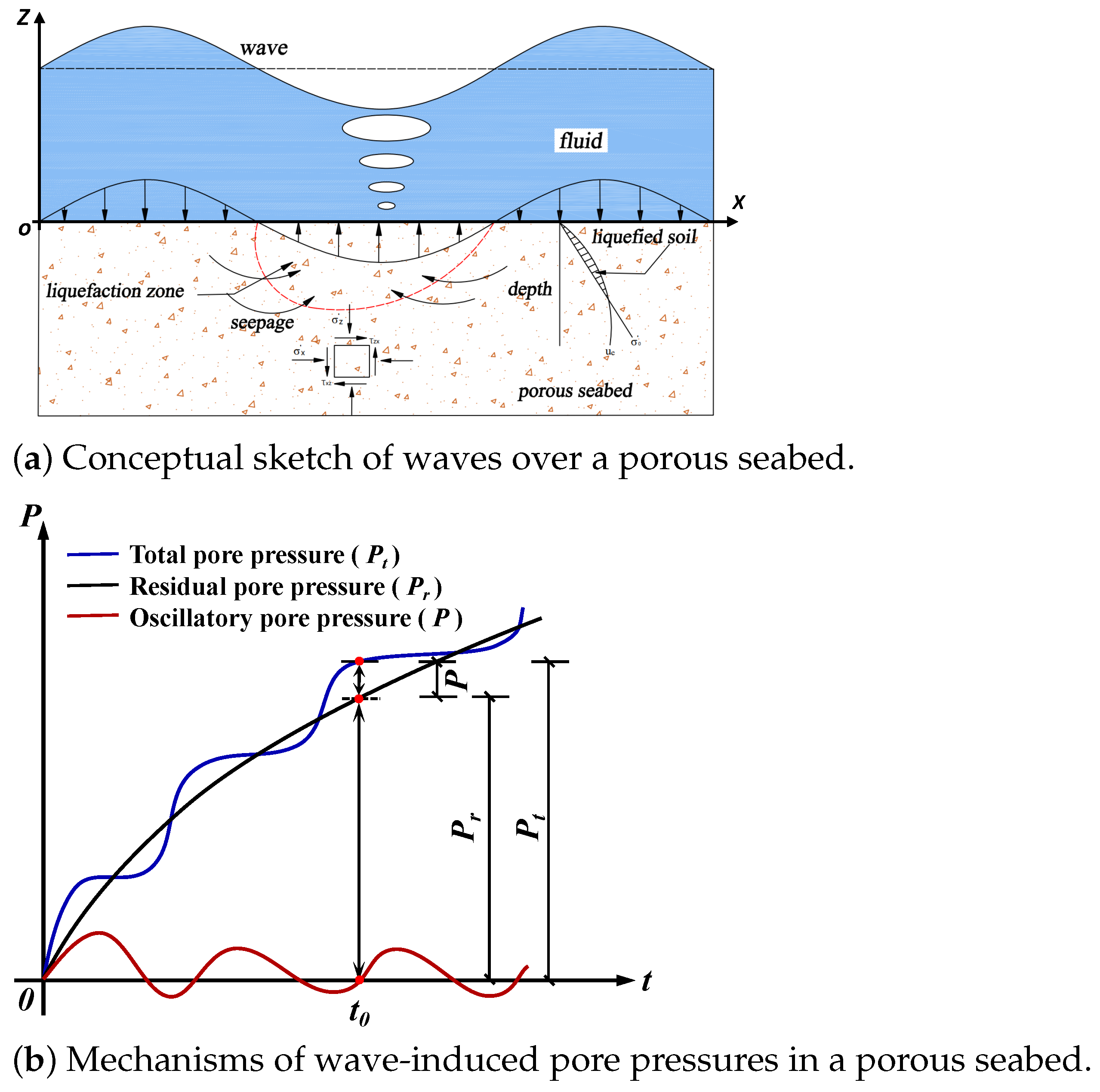
1. Introduction
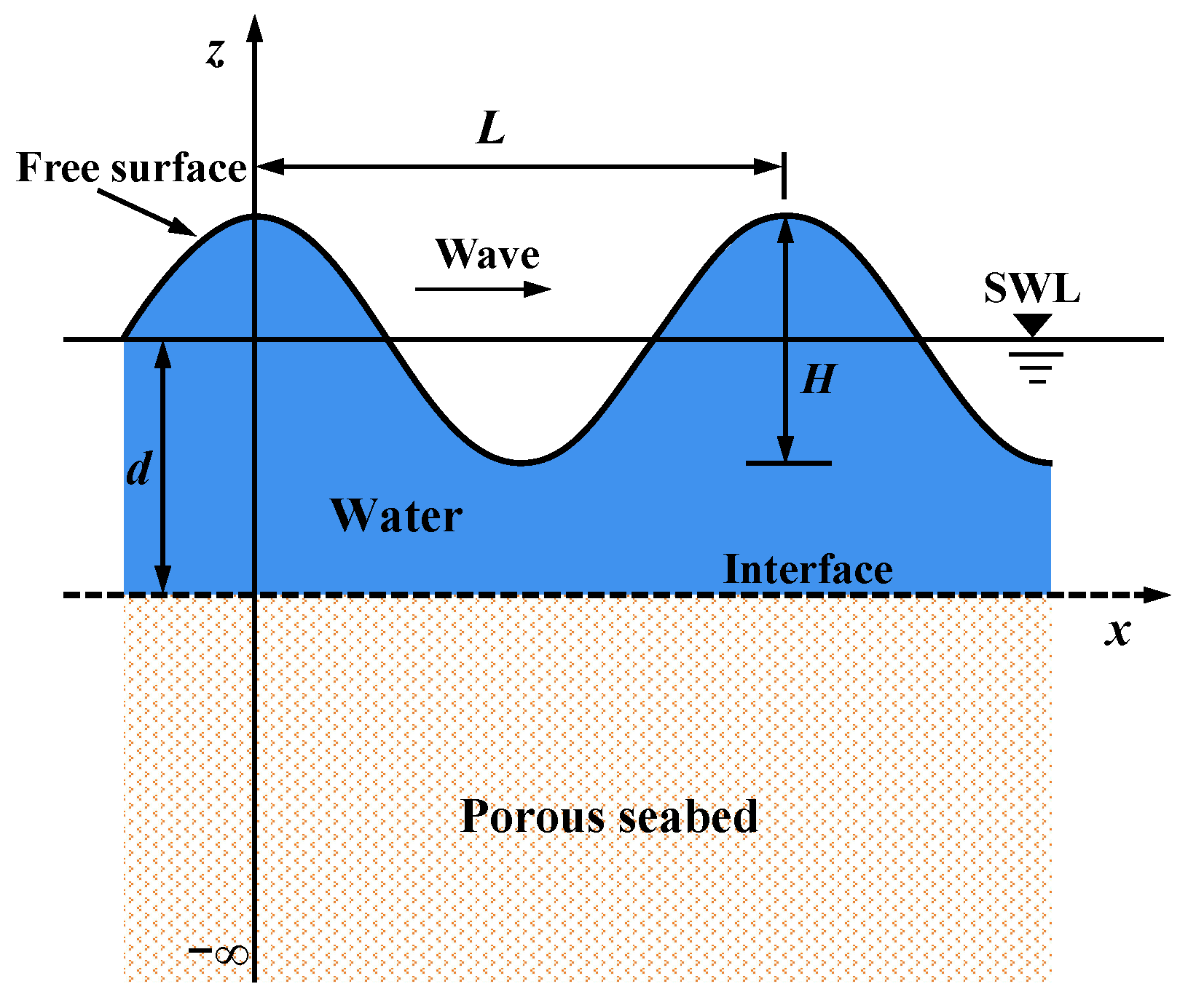
2. Analytical Solution for Wave-Induced Soil Response
3. Phase-Lag for Soil Response Variables
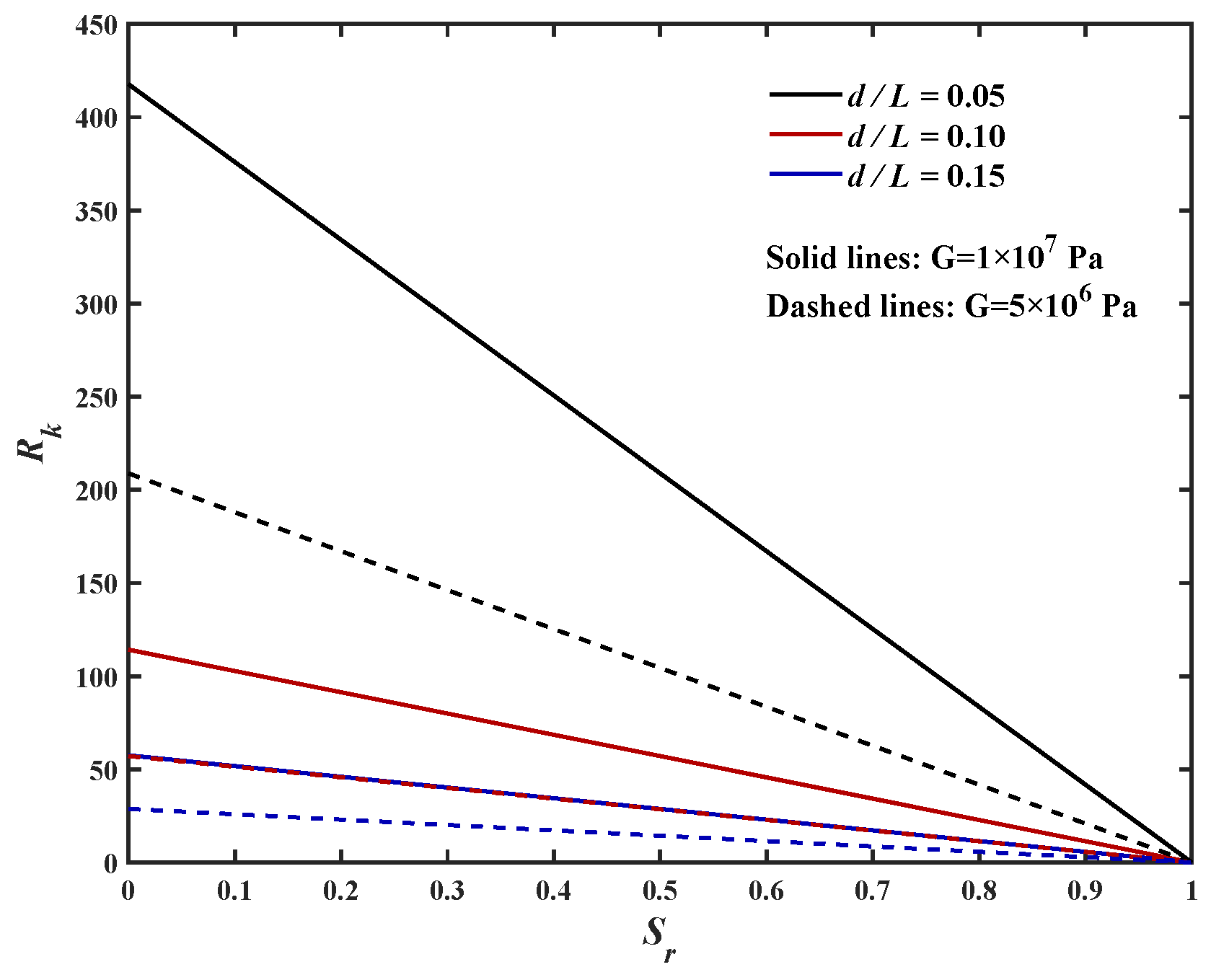
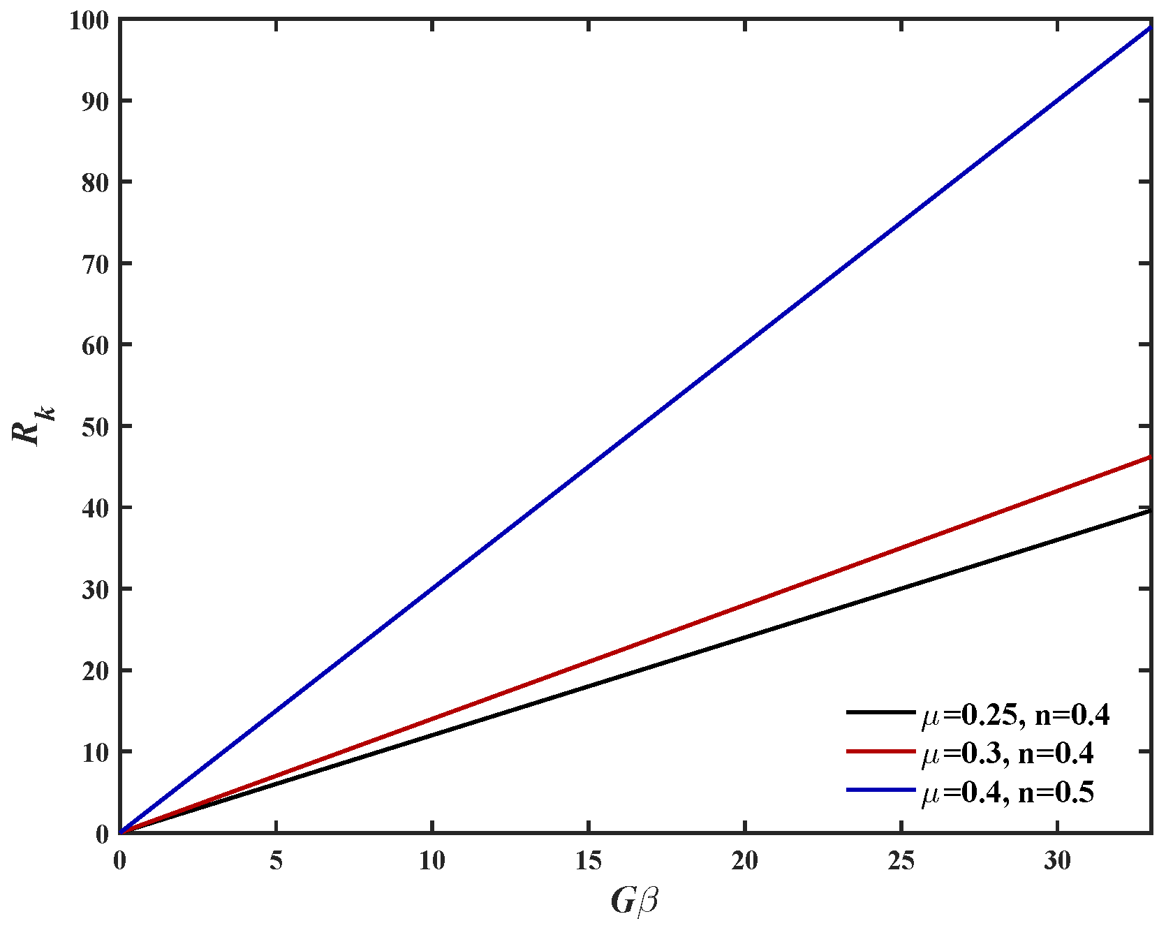
3.1. Relative Rigidity Parameter ()
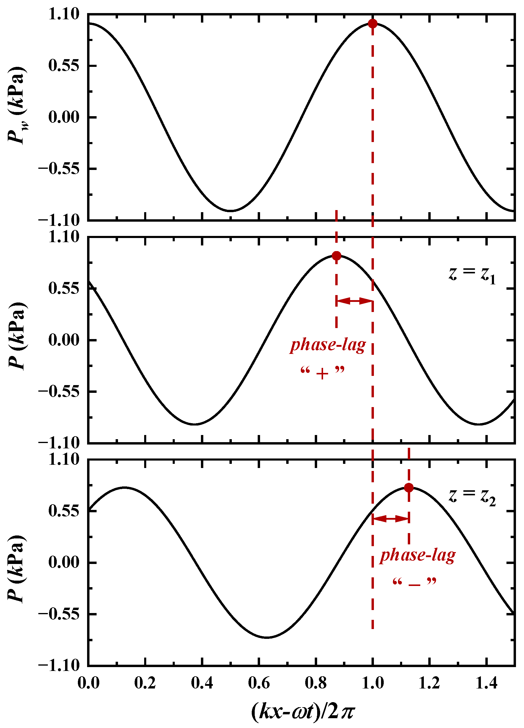
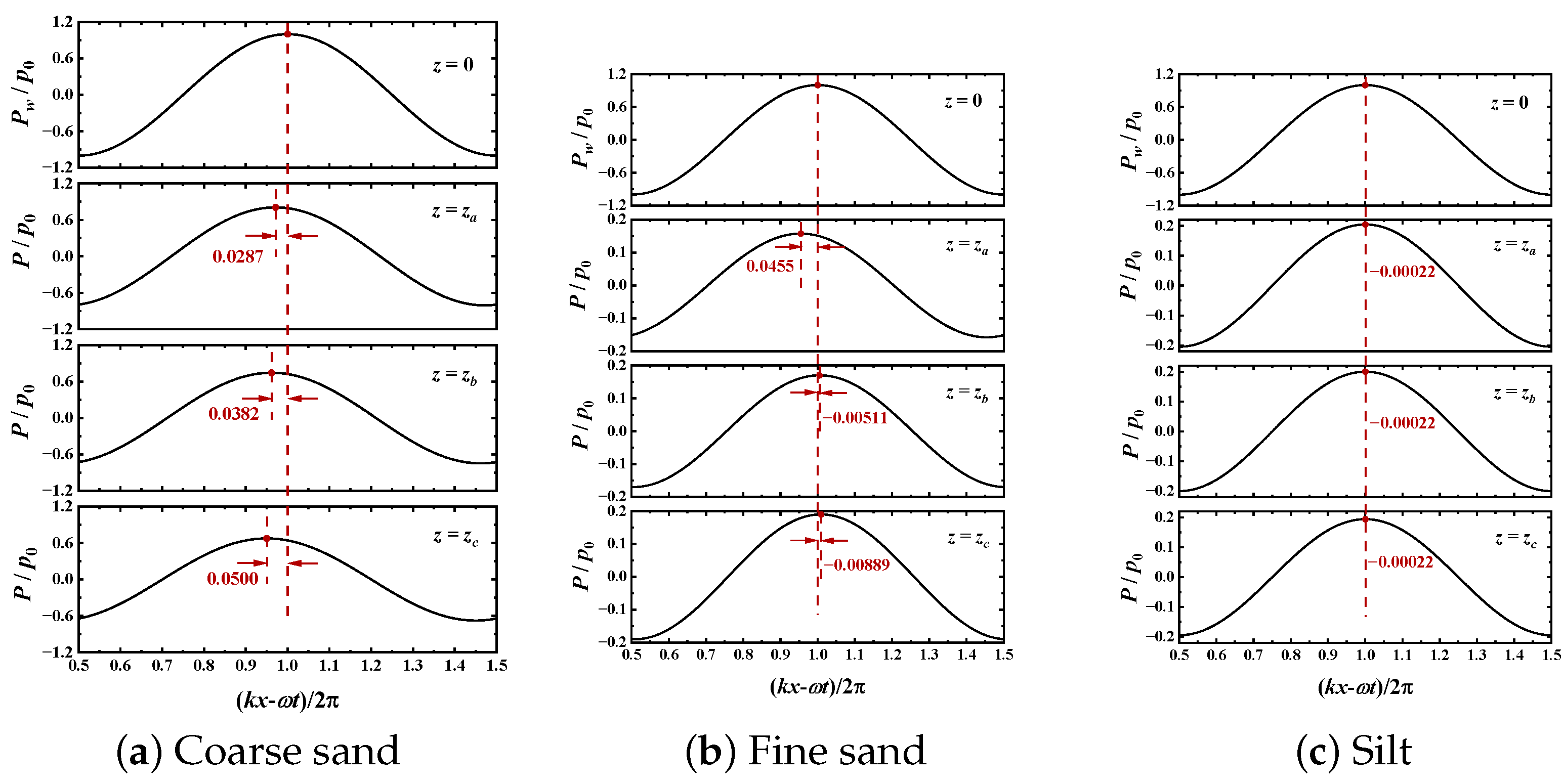
3.2. Phase-Lag for Pore Pressure (P)
- (1)
- Case-I:
- (2)
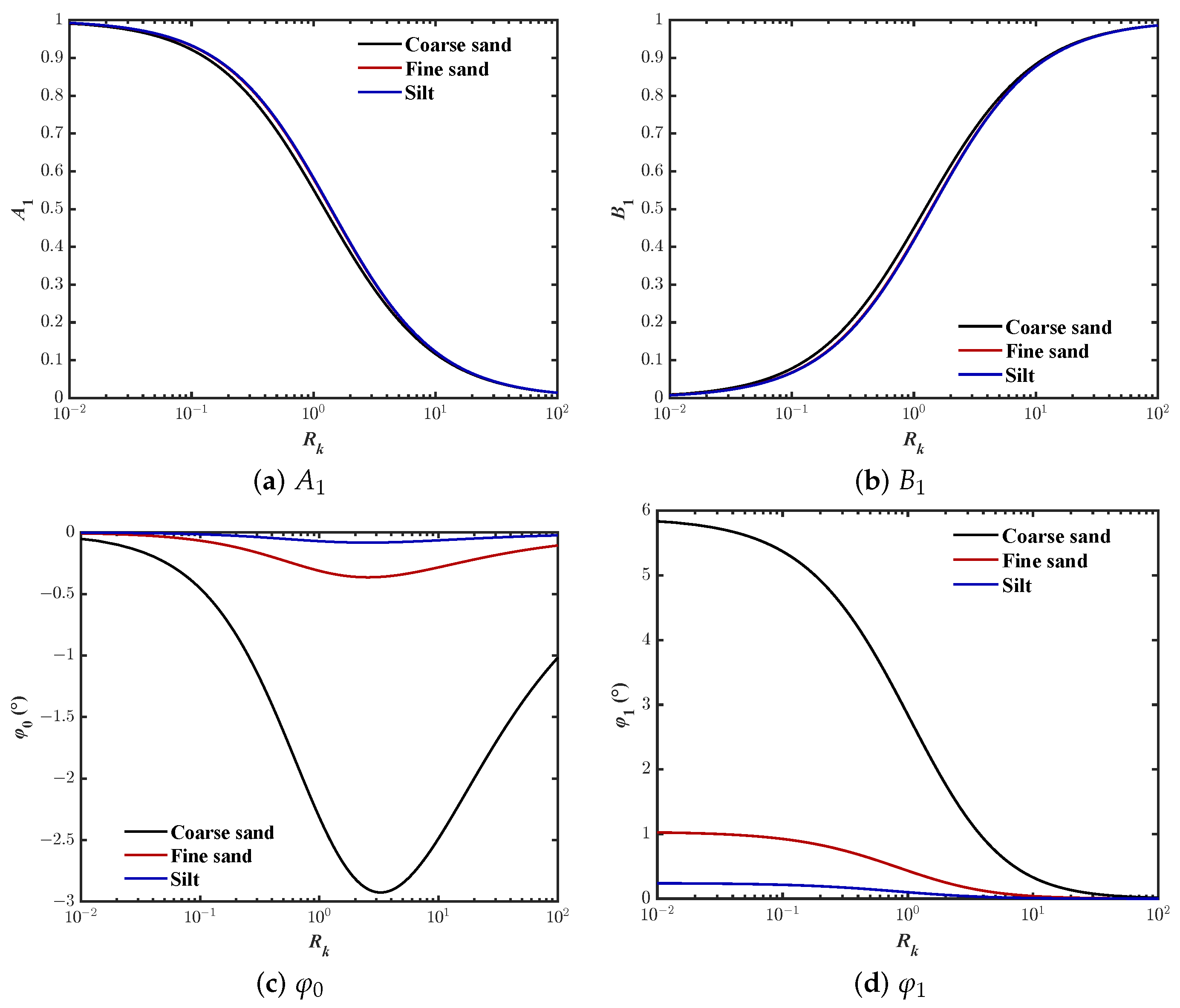
- Case-II:As shown in Figure 6, for , the coefficients approaches zero, approaches 1.0, and approaches zero when . That is,where the phase-lag for the wave-induced pore pressure can be expressed aswhich is a function of soil depth (z).
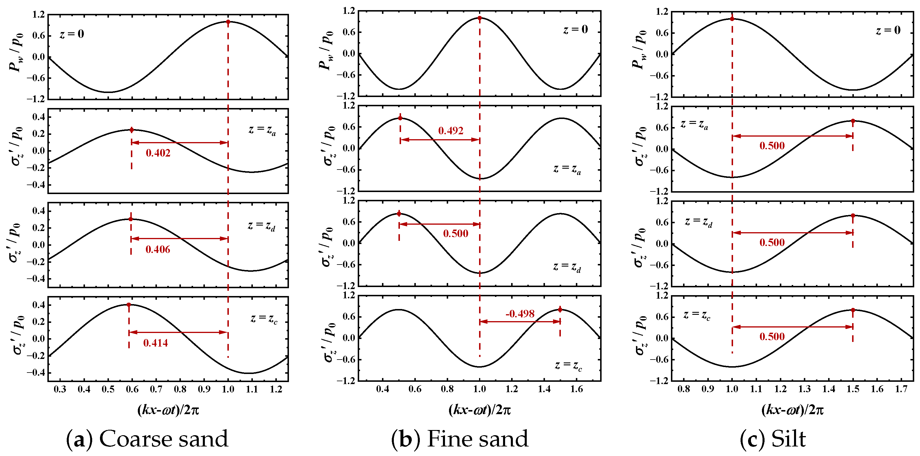
3.3. Phase-Lag for Effective Normal Stresses (, )
- (1)
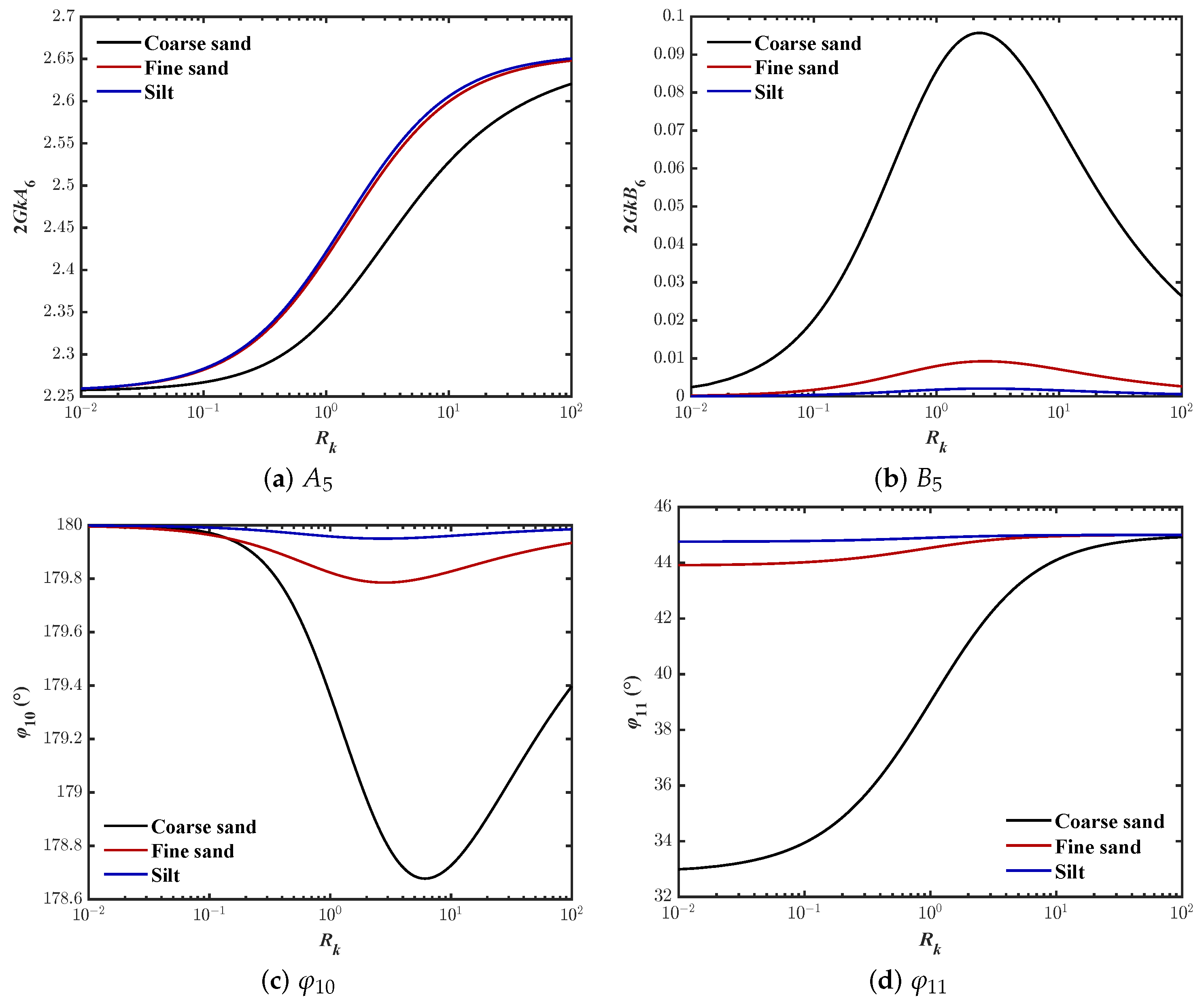
- Case-I:As shown in Figure 8, if , the coefficient approaches a constant, but the constant varies with the different parameters and approaches zero. Therefore,According to (55), the effective horizontal stress does not have phase delay in a fully saturated seabed.
- (2)
- Case-II:
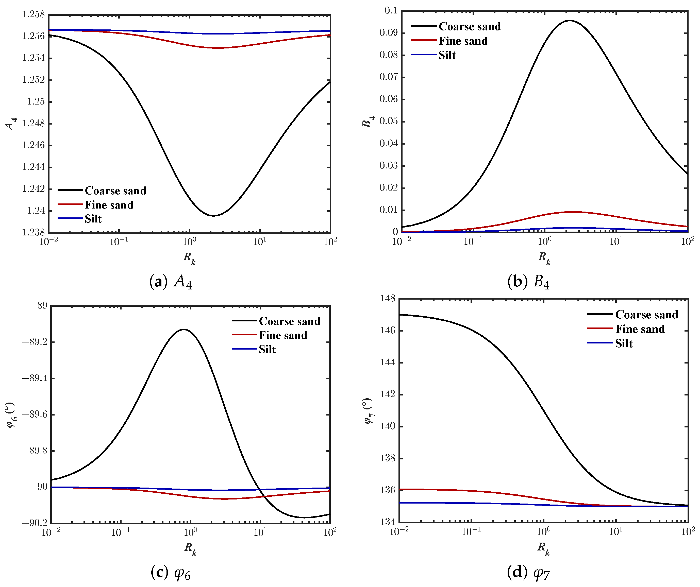
- (1)
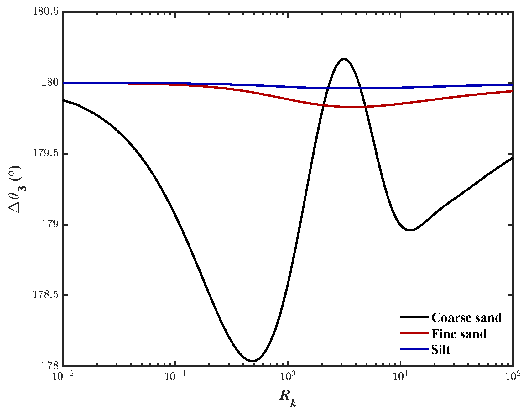
- Case-I:As shown in Figure 10, if , approaches a constant, while approaches zero and approaches 180 degrees. Therefore, (58) can be simplified toAccording to (69), when the seabed is fully saturated, the phase-lag for the effective vertical stress is 180 degrees.
- (2)
- Case-II:As shown in Figure 10, when , approaches a constant, approaches 1.0, and approaches 0 degrees. That iswhere the phase-lag for the effective vertical stress can be expressed as
3.4. Phase-Lag for Shear Stress ()
- (1)
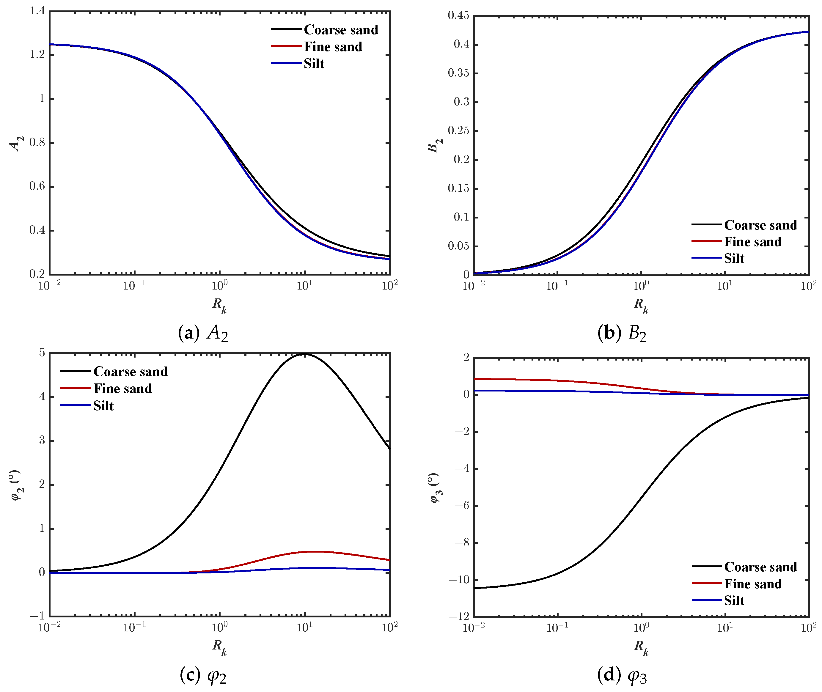
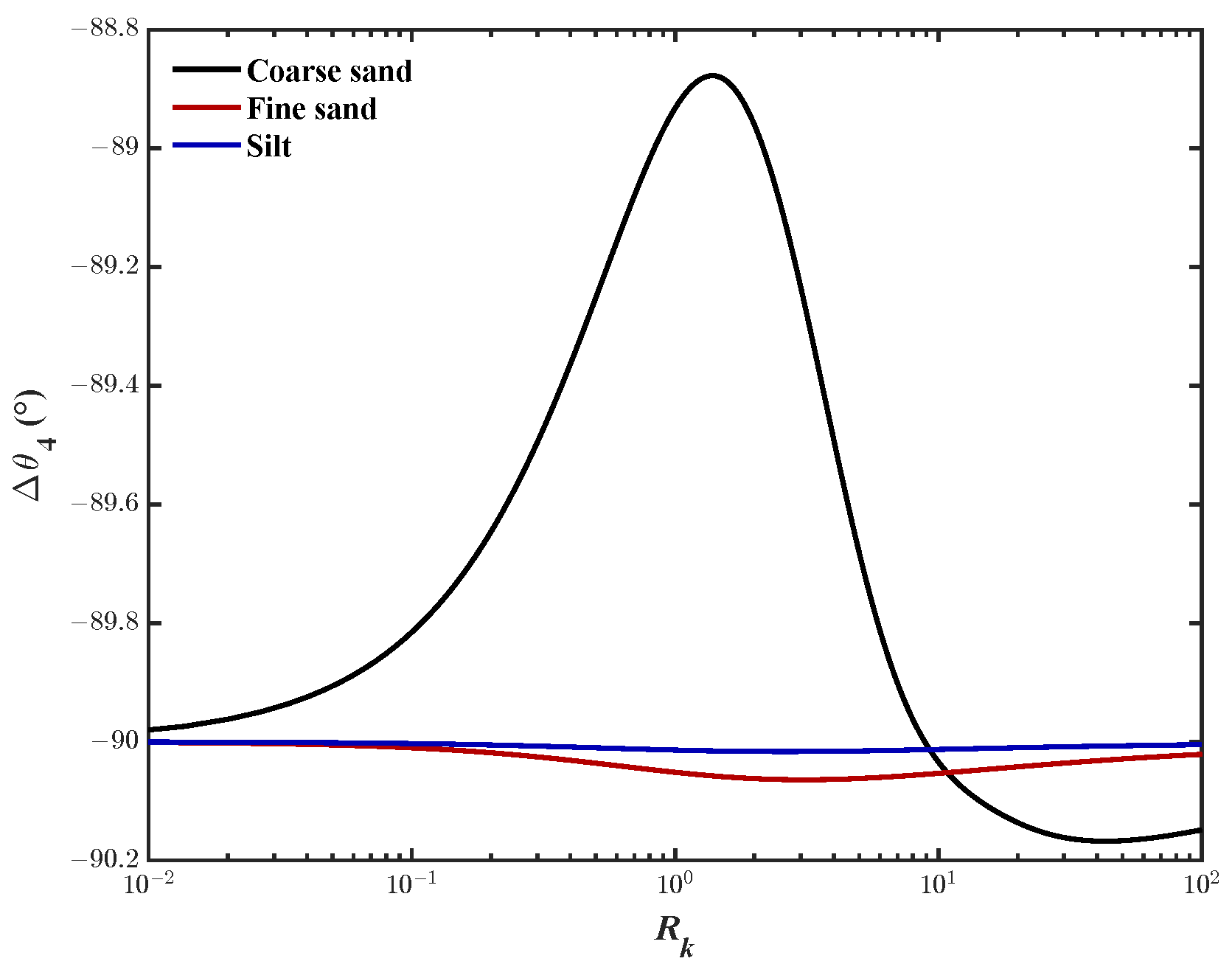
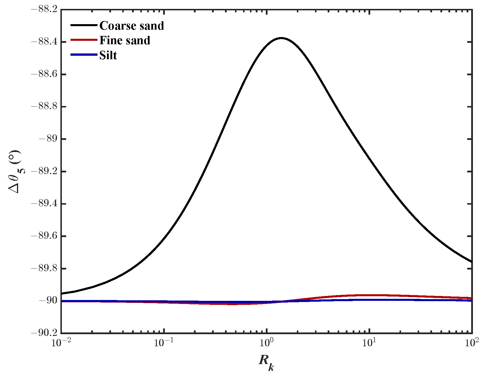
- Case-I:As shown in Figure 12, for this case, cannot be ignored, approaches zero, and approaches −90 degrees. Then, (72) can be simplified toFrom (82), when , the phase-lag for shear stress is −90 degrees.
- (2)
- Case-II:When , is much smaller than , so the second term can be neglected. Then, (72) can be simplified toand the phase-lag for shear stress can be calculated by
3.5. Phase-Lag for Soil Displacements (u, w)
- (1)
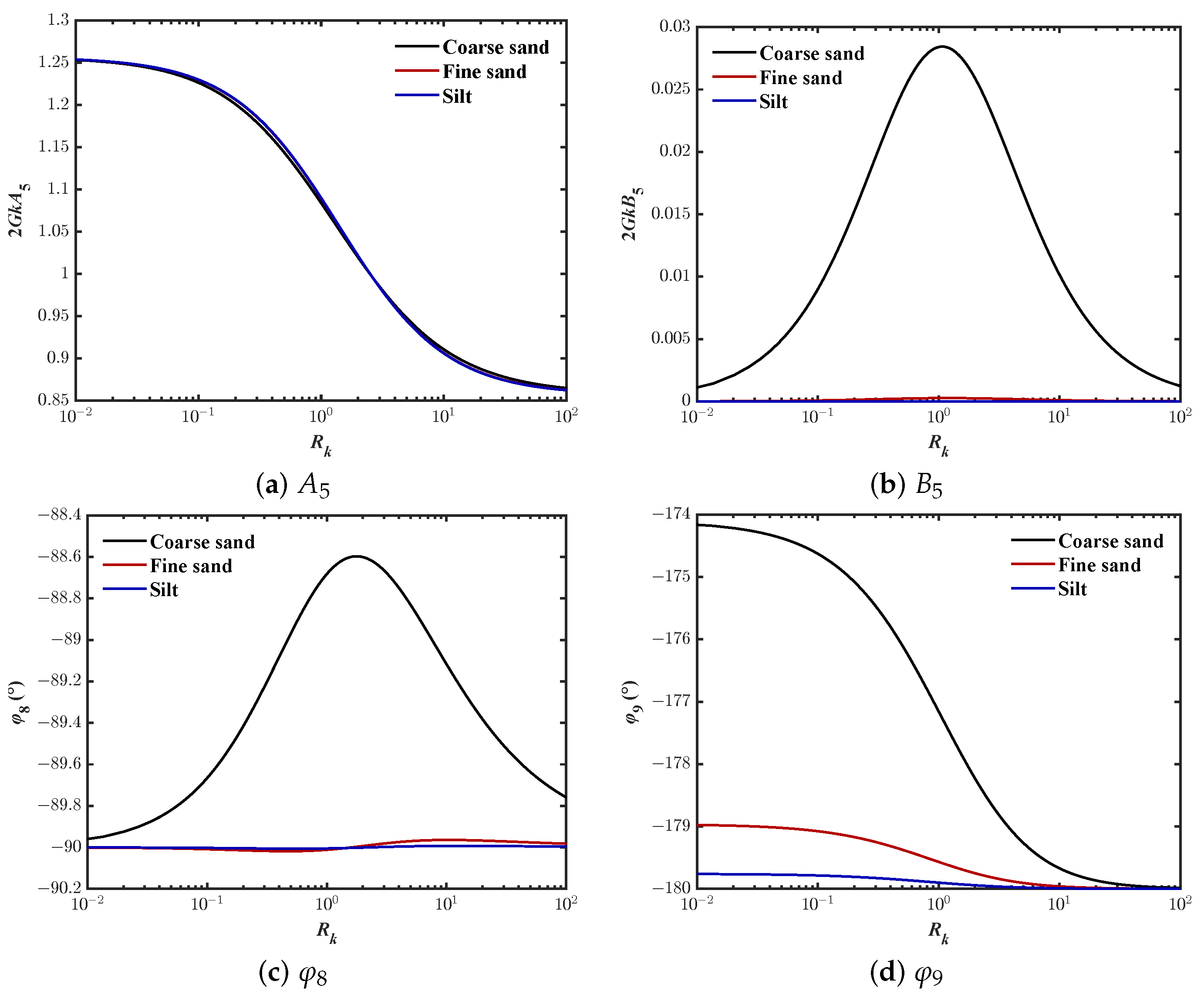
- Case-I:As illustrated in Figure 14, when , approaches the constant, approaches zero, and approaches . (85) can be simplified toFrom (94), when , the phase-lag for x-displacement is −90 degrees.
- (2)
- Case-II:If , is also much smaller than , and approaches zero (see Figure 14). That isand the phase-lag for soil displacement in x-direction can be expressed as
- (1)
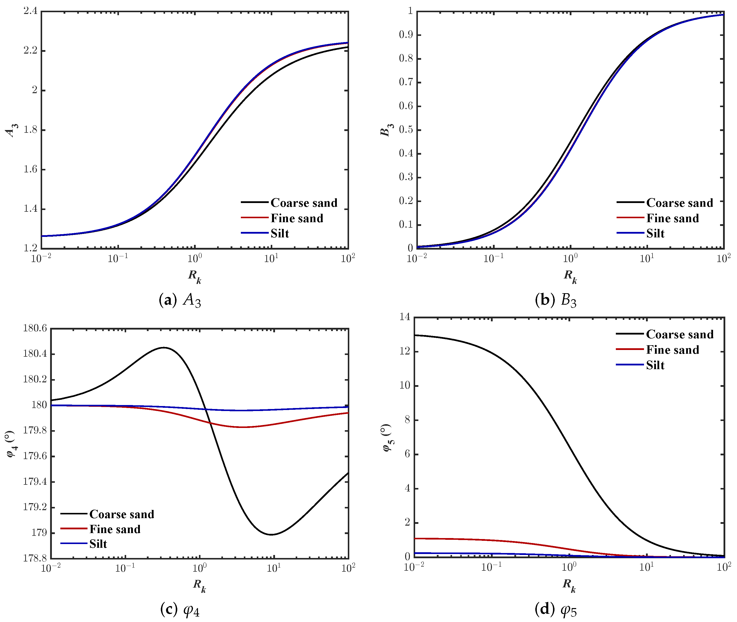
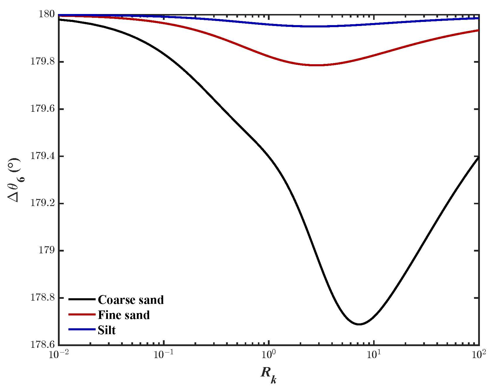
- Case-I:When , approaches a constant, approaches zero, and approaches as seen in Figure 16. Then, (97) can be simplified toFrom (106), in this case, the phase-lag is 180 degrees.
- (2)
- Case-II:If , is much smaller than , so the second term can be ignored (see Figure 16). That isand the phase-lag for vertical displacement can be expressed as
4. Parametric Study for Phase-Lags
4.1. Wave-Induced Pore Pressures (P)
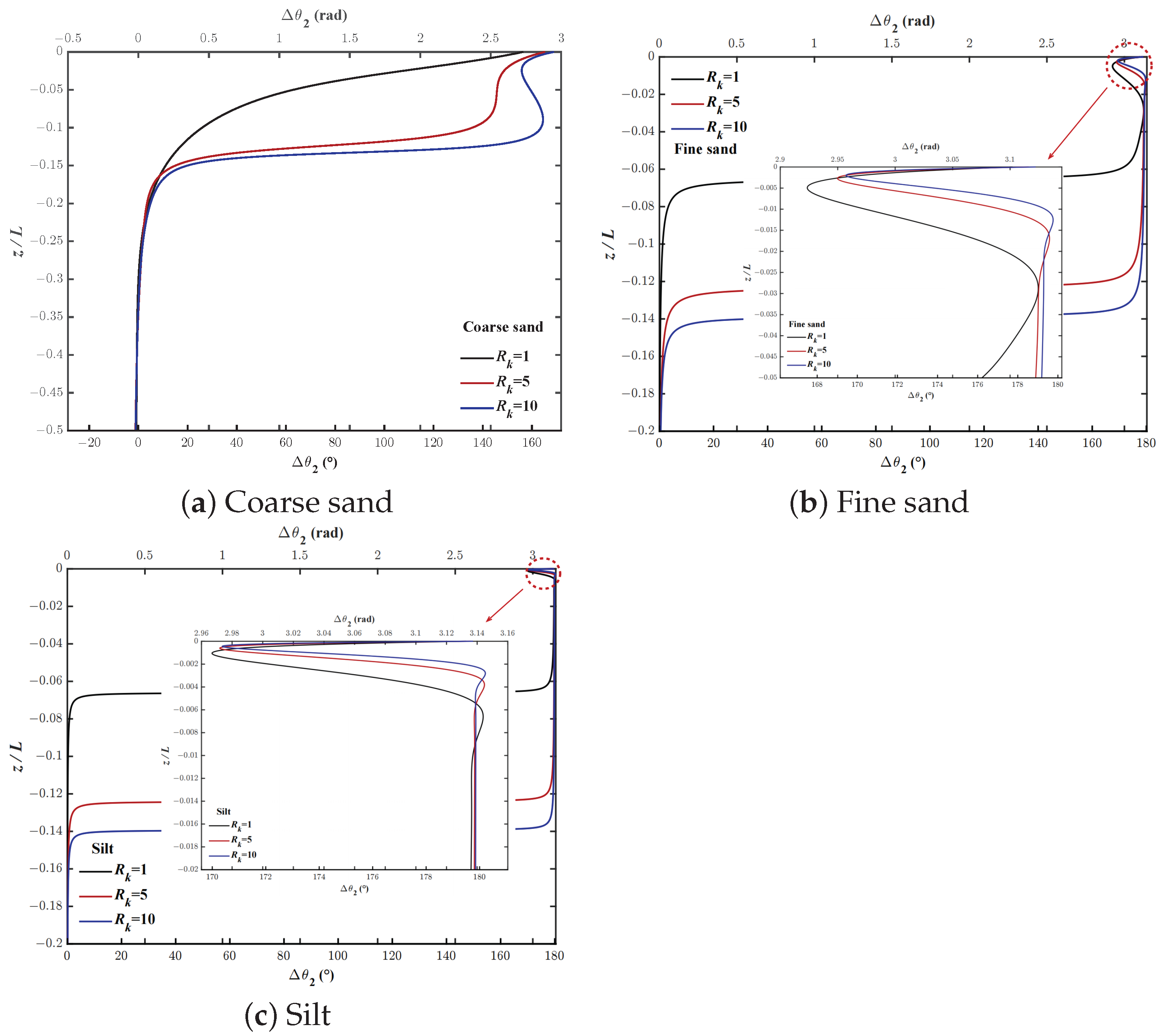
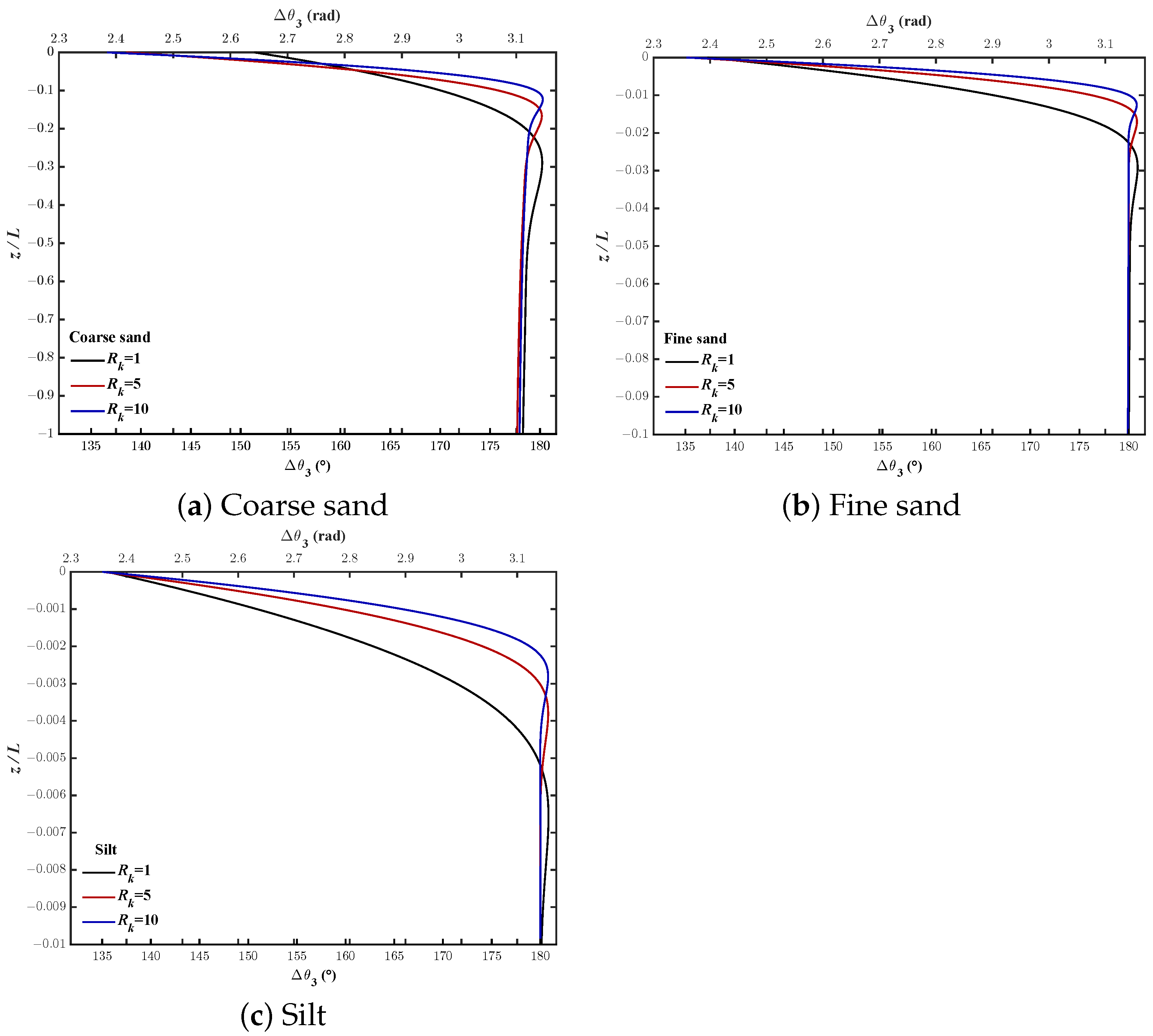
4.2. Wave-Induced Stress (, and )
5. Wave-Induced Seabed Stability
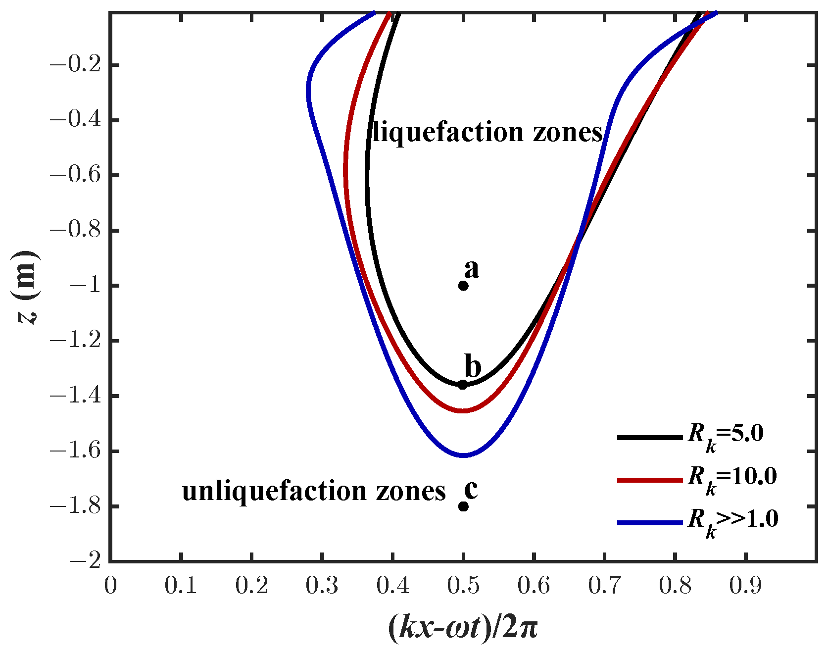
5.1. Liquefaction
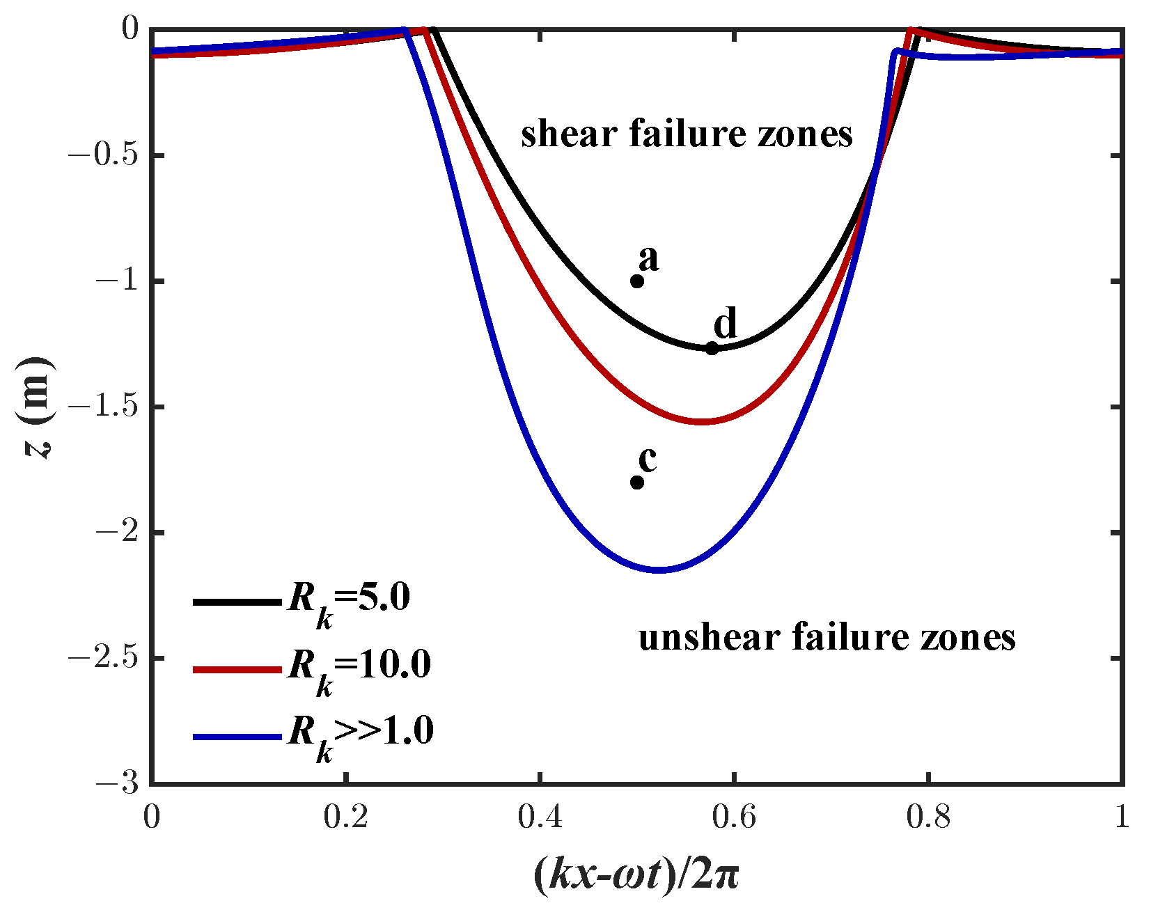
5.2. Shear Failure
6. Conclusions
- When the seabed is completely saturated, there are no phase-lags for wave-induced pore pressure and horizontal effective stress. However, the phase-lags for vertical effective stress and z-displacement are 180 degrees, and the phase-lags for shear stress and x-displacement are −90 degrees.
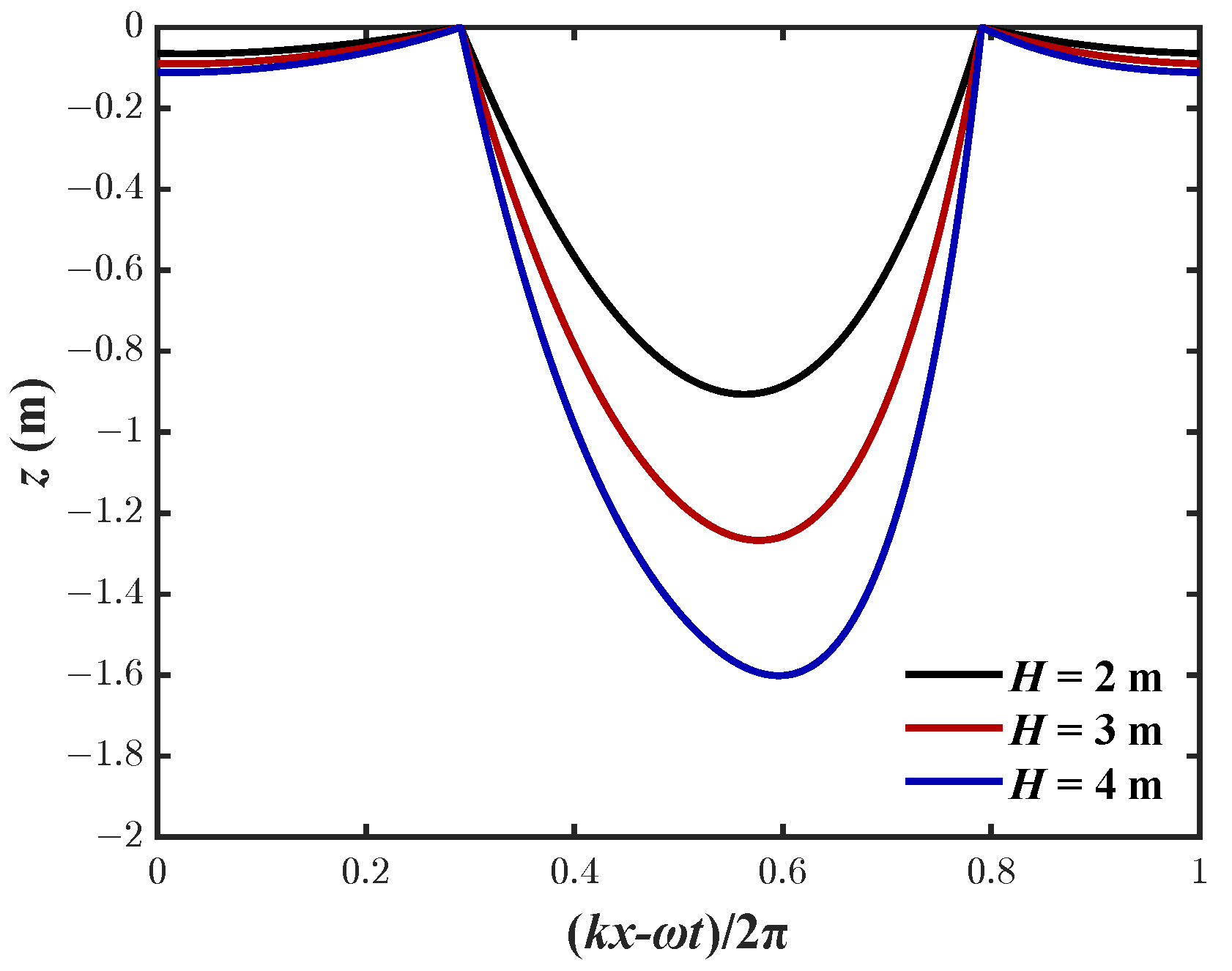
- The instantaneous liquefaction zone and shear failure zone increase with increasing . In addition, the liquefaction zone and the maximum liquefaction depth, as well as the shear failure zone and the maximum shear failure depth. Both increase with increasing wave height H.
- The phase-lag for wave-induced pore pressure increases with increasing . In contrast, the extreme phase delay for horizontal effective stress and shear stress decreases with increasing .
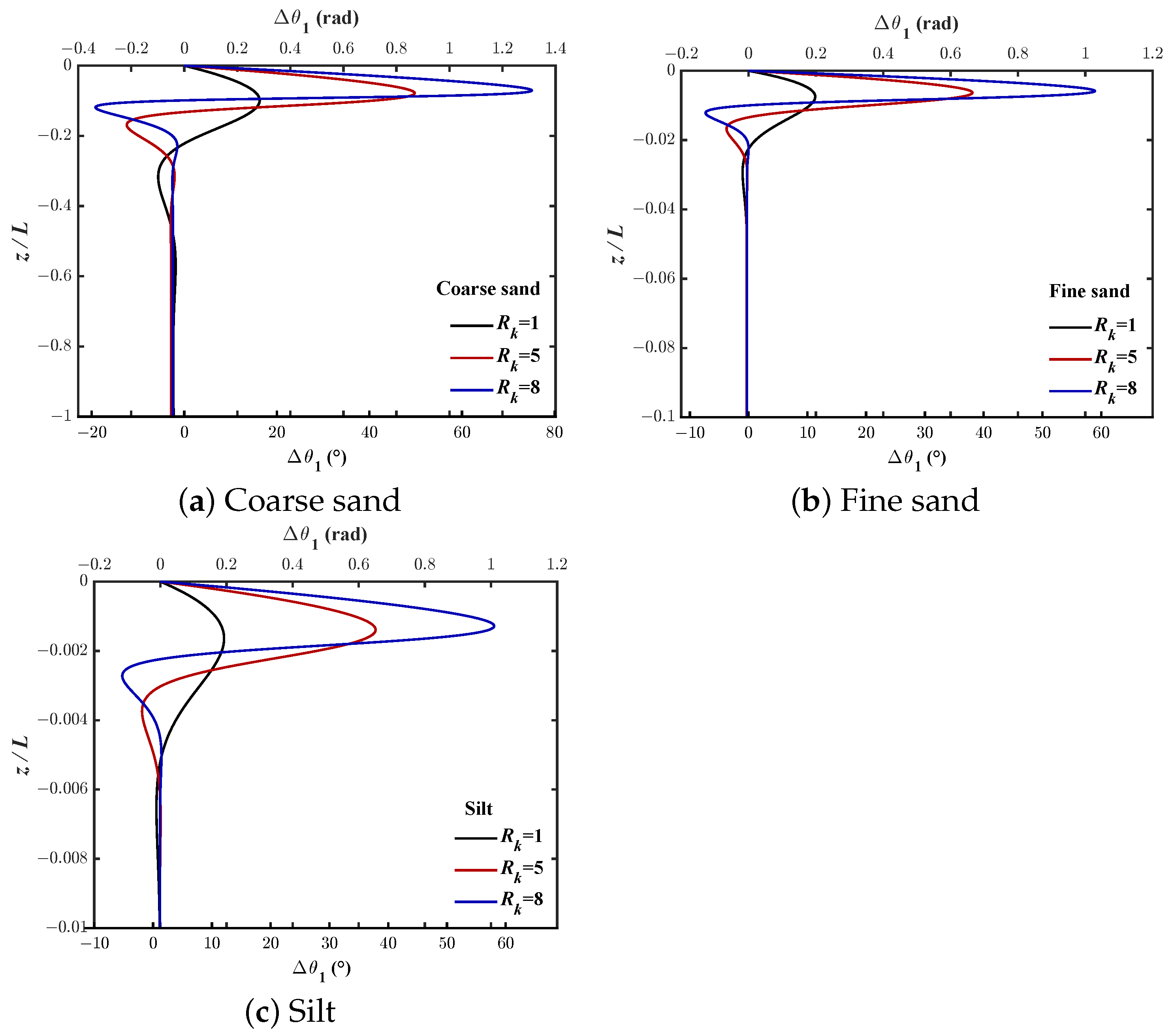
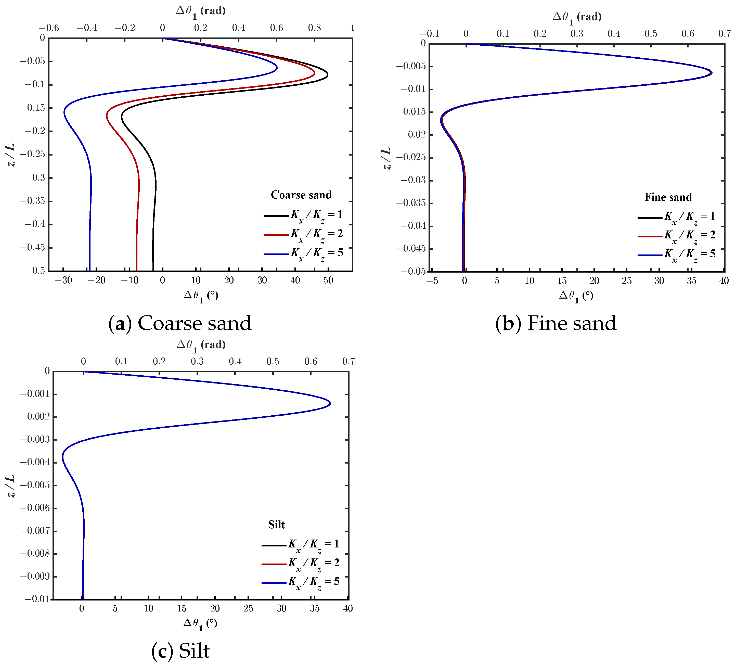
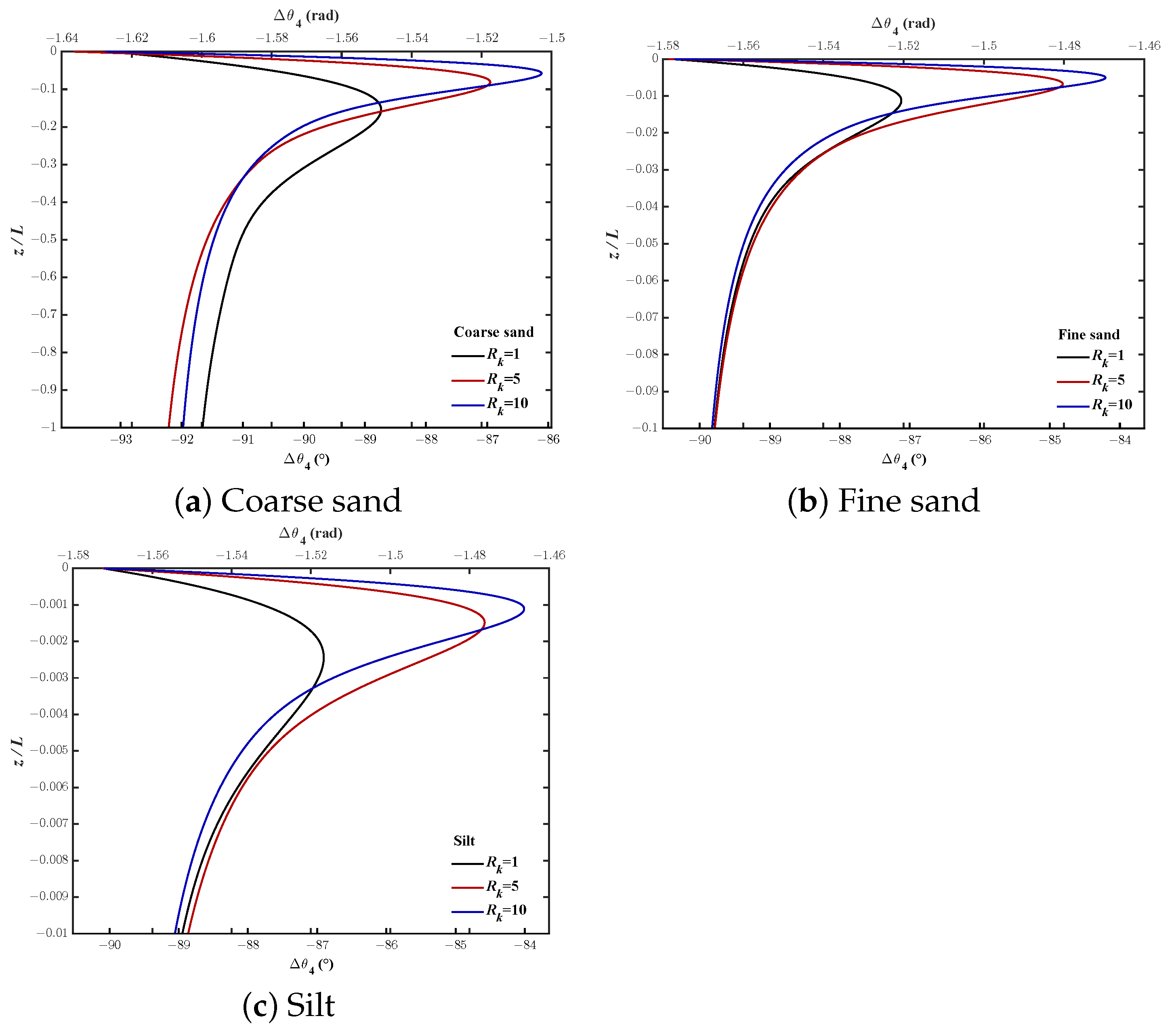
- When , in fine sand and silt, has almost no influence on phase-lag. In coarse sand, the phase-lag for wave-induced pore pressure and shear stress decreases with increasing , while the phase-lag for effective normal stresses is opposite.
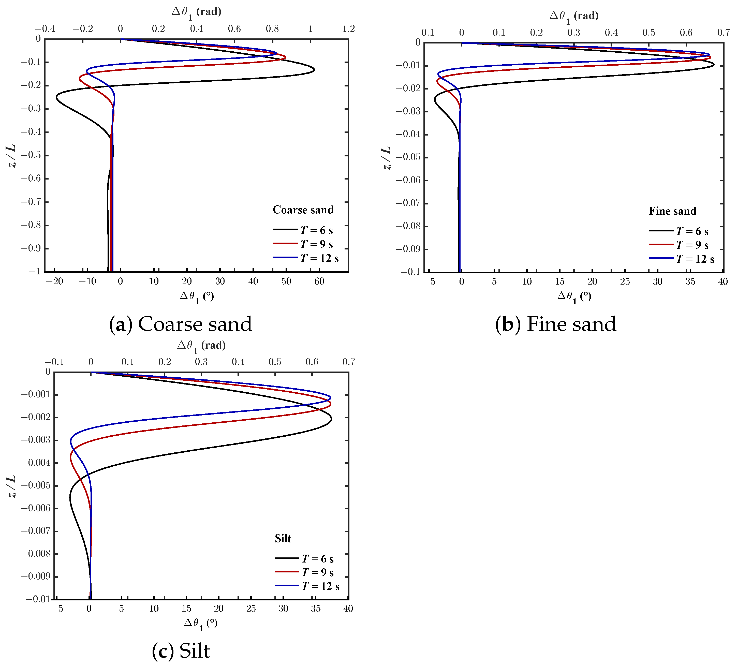
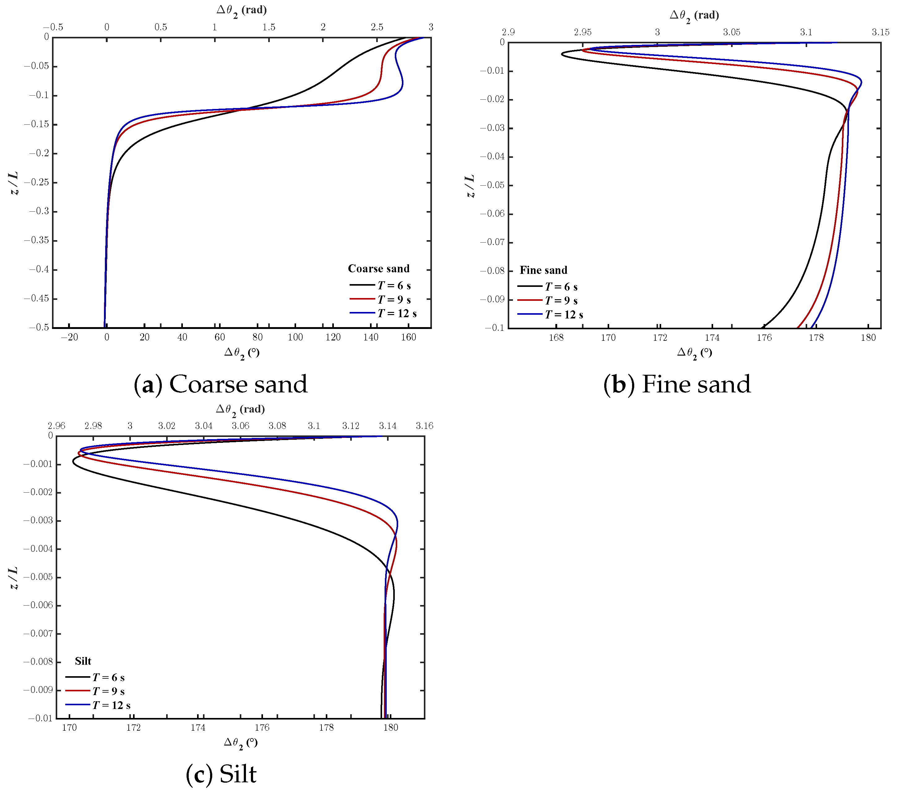
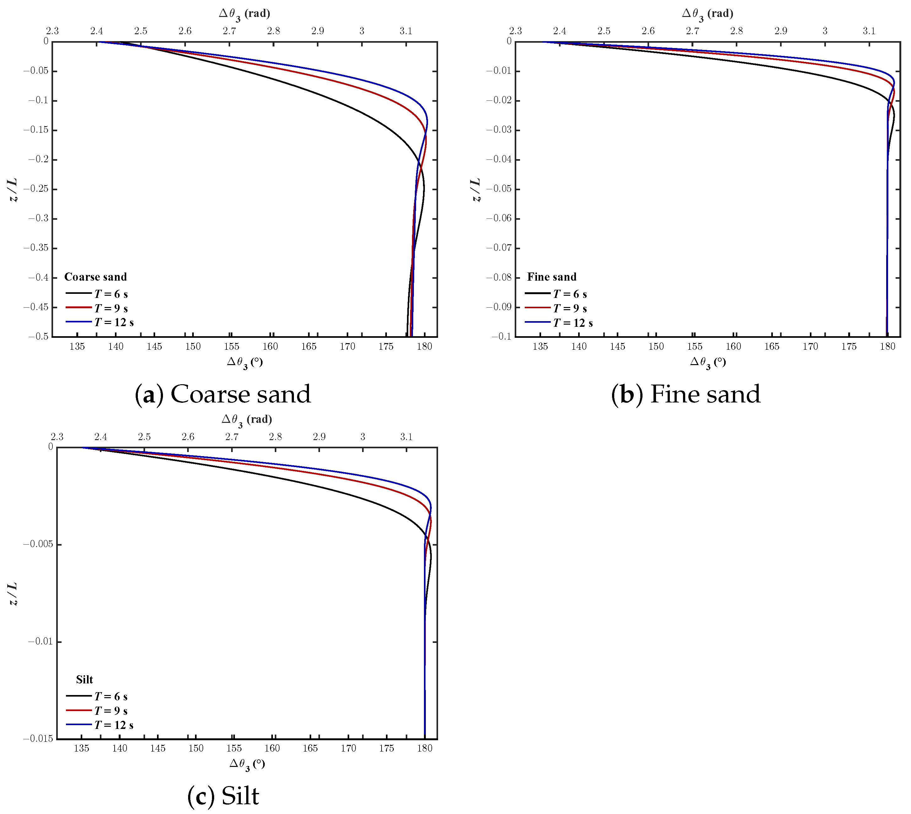
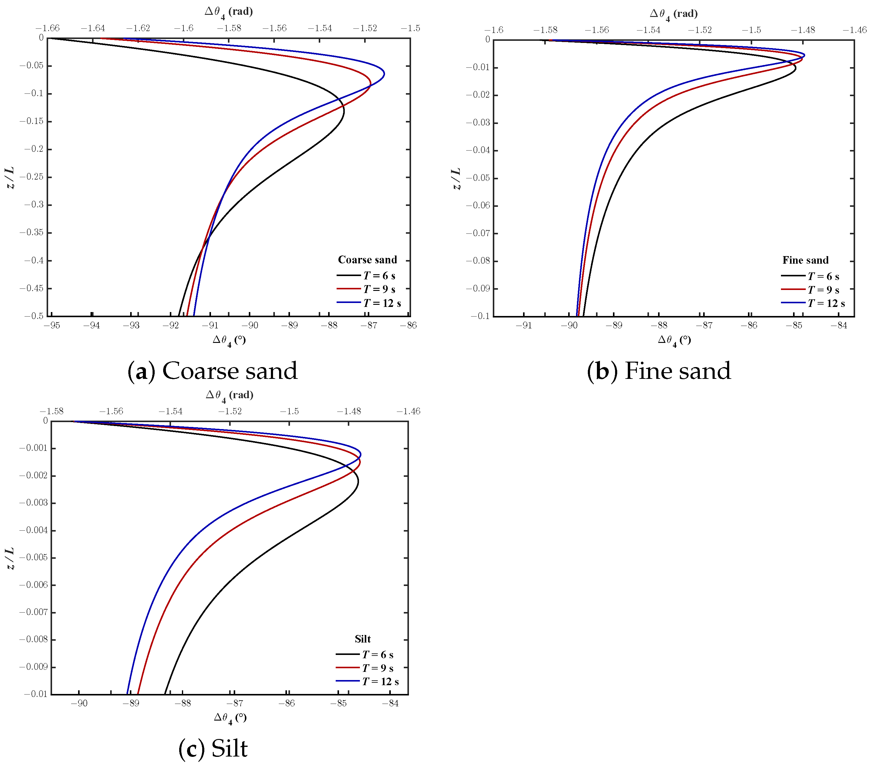
- The phase-lag for wave-induced pore pressure and shear stress decreases with increasing T, while the phase-lag for effective normal stresses is opposite. Moreover, the shorter the wave period, the deeper the soil depth affected by the phase-lag.
Author Contributions
Funding
Data Availability Statement
Acknowledgments
Conflicts of Interest
References
- Lundgren, H.; Lindhardt, J.H.C.; Romold, C.J. Stability of breakwaters on porous foundation. In Proceedings of the 12th International Conference on Soil Mechanics and Foundation Engineering, Rio de Janeiro, Brazil, 13–18 August 1989; Volume 1, pp. 451–454. [Google Scholar]
- Sumer, B.M.; Fredsøe, J. The Mechanics of Scour in the Marine Environment; World Scientific Publishing Company: Singapore, 2002; Volume 17. [Google Scholar] [CrossRef]
- Chung, S.G.; Kim, S.K.; Kang, Y.J.; Im, J.C.; Prasad, K.N. Failure of a breakwater founded on a thick normally consolidated clay layer. Géotechnique 2006, 56, 393–409. [Google Scholar] [CrossRef]
- Zen, K.; Yamazaki, H. Mechanism of wave-induced liquefaction and densification in seabed. Soils Found. 1990, 30, 90–104. [Google Scholar] [CrossRef] [PubMed]
- Nago, H.; Maeno, S.; Matsumoto, T.; Hachiman, Y. Liquefaction and densification of loosely deposited sand bed under water pressure variation. In Proceedings of the the 3rd International Offshore and Polar Engineering Conference (ISOPE1993), Singapore, 6–11 June 1993; Volume I, pp. 578–584. [Google Scholar]
- Sumer, B.M. Liquefaction around Marine Structures. Adv. Ser. Ocean. Eng. 2014, 39. [Google Scholar] [CrossRef]
- Wan, Z.P.; Cui, L.; Jeng, D.S. Integrated model for wave-induced oscillatory and residual soil response in a poro-elastic seabed: Partially dynamic model. J. Mar. Sci. Eng. 2023, 11, 833. [Google Scholar] [CrossRef]
- Sleath, J.F.A. Wave-induced pressures in beds of sand. J. Hydraul. Div. ASCE 1970, 96, 367–378. [Google Scholar] [CrossRef]
- Okusa, S. Wave-induced stress in unsaturated submarine sediments. Géotechnique 1985, 35, 517–532. [Google Scholar] [CrossRef]
- Tsui, Y.T.; Helfrich, S.C. Wave-induced pore pressures in submerged sand layer. J. Geotech. Eng. ASCE 1983, 109, 603–618. [Google Scholar] [CrossRef]
- Liu, B.; Jeng, D.S.; Ye, G.L.; Yang, B. Laboratory study for pore pressures in sandy deposit under wave loading. Ocean. Eng. 2015, 106, 207–219. [Google Scholar] [CrossRef]
- Yamamoto, T.; Koning, H.; Sellmeijer, H.; Hijum, E.V. On the response of a poro-elastic bed to water waves. J. Fluid Mech. 1978, 87, 193–206. [Google Scholar] [CrossRef]
- Li, C.F.; Gao, F. Characterization of spatio-temporal distributionof wave-induced pore pressure in a non-cohesive seabed: Amplitude-attenuation and phase-lag. Ocean. Eng. 2022, 253, 111315. [Google Scholar] [CrossRef]
- Li, C.F.; Yu, J.H.; Gao, F.P. Phase-lag effect on the instantaneously-liquefied seabed depth under progressive waves: Explicit approximations. Appl. Ocean. Res. 2024, 147, 103965. [Google Scholar] [CrossRef]
- Zen, K.; Jeng, D.S.; Hsu, J.R.C.; Ohyama, T. Wave-induced seabed instability: Difference between liquefaction and shear failure. Soils Found. 1998, 38, 37–47. [Google Scholar] [CrossRef] [PubMed]
- Hsu, J.R.C.; Jeng, D.S.; Tsai, C.P. Short-crested wave-induced soil response in a porous seabed of infinite thickness. Int. J. Numer. Anal. Methods Geomech. 1993, 17, 553–576. [Google Scholar] [CrossRef]
- Darcy, H. Les Fontaines Publiques de la Ville de Dijon; Dalmont, V., Ed.; Calilas-Gary and First Damalute: Paris, France, 1856; Volume 1. [Google Scholar]
- Dean, R.; Dalrymple, R.A. Water wave mechanics for engineers and scientists. Adv. Ser. Ocean. Eng. 1984, 2, 253. [Google Scholar] [CrossRef]
- Cui, L.; Jeng, D.S. Two-dimensional one-way coupled modelling for fluid-structure-seabed interactions around a semicircular breakwater using OpenFOAM. Appl. Ocean. Res. 2024, 153, 104249. [Google Scholar] [CrossRef]
- Mei, C.C.; Foda, M.A. Wave-induced response in a fluid-filled poro-elastic solid with a free surface-a boundary layer theory. Geophys. J. R. Astron. Soc. 1981, 66, 597–631. [Google Scholar] [CrossRef]
- Scott, R.F. Principle of Soil Mechanics; Addison-Publishing Company INC.: London, UK, 1963. [Google Scholar]


| Wave Parameters | Value | ||
|---|---|---|---|
| Wave period (T) [s] | 9.0 | ||
| Water depth (d) [m] | 15.0 | ||
| Wave height (H) [m] | 3.0 | ||
| Wave length (L) [m] | 95.5 | ||
| Soil properties | Coarse sand | Fine sand | Silt |
| Permeability (, ) [m/s] | |||
| Shear modulus (G) [Pa] | |||
| Poisson’s ratio () [-] | 0.3 | ||
| Porosity (n) [-] | 0.4 | ||
Disclaimer/Publisher’s Note: The statements, opinions and data contained in all publications are solely those of the individual author(s) and contributor(s) and not of MDPI and/or the editor(s). MDPI and/or the editor(s) disclaim responsibility for any injury to people or property resulting from any ideas, methods, instructions or products referred to in the content. |
© 2025 by the authors. Licensee MDPI, Basel, Switzerland. This article is an open access article distributed under the terms and conditions of the Creative Commons Attribution (CC BY) license (https://creativecommons.org/licenses/by/4.0/).
Share and Cite
He, X.; Jeng, D.-S. Wave-Induced Seabed Stability in an Infinite Porous Seabed: Effects of Phase-Lags. J. Mar. Sci. Eng. 2025, 13, 1397. https://doi.org/10.3390/jmse13081397
He X, Jeng D-S. Wave-Induced Seabed Stability in an Infinite Porous Seabed: Effects of Phase-Lags. Journal of Marine Science and Engineering. 2025; 13(8):1397. https://doi.org/10.3390/jmse13081397
Chicago/Turabian StyleHe, Xufen, and Dong-Sheng Jeng. 2025. "Wave-Induced Seabed Stability in an Infinite Porous Seabed: Effects of Phase-Lags" Journal of Marine Science and Engineering 13, no. 8: 1397. https://doi.org/10.3390/jmse13081397
APA StyleHe, X., & Jeng, D.-S. (2025). Wave-Induced Seabed Stability in an Infinite Porous Seabed: Effects of Phase-Lags. Journal of Marine Science and Engineering, 13(8), 1397. https://doi.org/10.3390/jmse13081397