Navigation Attitude Prediction for Unmanned Surface Vessels in Wave Environments Using Improved Unscented Kalman Filter and Digital Twin Model

Abstract

Unmanned surface vehicles (USVs) face significant challenges in long-term operations in complex and dynamic marine environments. These include abnormal attitudes, low accuracy in navigation attitude prediction, and difficulties in maintaining operational stability and equipment safety. To address these issues, this paper proposed a USV navigation attitude prediction method that integrates Unscented Kalman Filtering (UKF) with a digital twin model. First, a three-degree-of-freedom mathematical model is constructed based on the motion characteristics of the USV to establish an initial digital twin model. Then, the UKF algorithm is improved with a dynamic sliding window approach and integrated with real vessel experimental data to achieve dynamic model parameter updates, further enhancing prediction accuracy. The updated twin model is subsequently used for USV navigation attitude prediction. Experimental results demonstrate that this method significantly improves prediction accuracy and robustness, even under complex sea conditions and sensor data loss, providing crucial support for the safety and reliability of USV autonomous navigation.

1. Introduction

In recent years, the rapid advancement of technology and the growing demand for marine applications have brought unmanned surface vehicles (USVs) into increasing prominence. As a new class of vessels, USVs are capable of operating autonomously or under remote control on the water’s surface without direct human intervention. They have become essential tools and platforms in various fields such as marine scientific research, resource exploration, environmental monitoring, maritime patrol, reconnaissance, mine sweeping, and maritime defense [1]. By extending the capabilities of traditional vessels, USVs offer improved operational flexibility, reduced human risk, and enhanced efficiency, making them vital assets in both civilian and military domains [2].

However, despite their growing importance, USVs face significant operational challenges, particularly when navigating in dynamic and unpredictable marine environments. Variations in wind speed and direction can impact their stability and path control, while waves and ocean currents often cause trajectory deviations, introducing complexity and uncertainty into their motion. Furthermore, high-precision navigation and positioning systems, critical for USV operations, can be severely affected by GPS (Global Positioning System) signal interference at sea, leading to increased positioning errors [3]. In such conditions, accurate navigation attitude prediction becomes crucial. By precisely forecasting the navigation attitude of USVs, it is possible to achieve high-precision motion control, optimize dynamic responses, and enhance hazard avoidance, thereby ensuring the safe and effective operation of USVs.

To ensure the safe operation of unmanned boats and the successful execution of specific tasks, many researchers worldwide have focused on the field of unmanned boat attitude prediction. However, the methods used are often cumbersome, with poor model generalization, making them difficult to apply to real vessels. Current methods for predicting unmanned boat motion are mainly divided into three categories: mathematical models, statistical models, and machine learning models [4].

Unmanned boats exhibit six degrees of freedom in motion when navigating in waves: pitch, roll, yaw, surge, sway, and heave. Carrillo S. et al. performed ship motion modeling based on the Nomoto model and determined the KT parameters using the least squares method [5]. L. W. Yu and others used a potential flow-based five-degree-of-freedom nonlinear time-domain model to quantitatively predict the roll of the KCS (KRISO Container Ship) container ship [6]. Z. Z. applied Support Vector Machine (SVM) to identify the hydrodynamic derivatives and moments in the Abkowitz model, thereby improving the accuracy of ship maneuvering prediction [7].

Common statistical prediction methods include regression analysis, gray theory, fuzzy theory, and time-series methods [8]. These statistical methods typically rely on large amounts of accurate input–output data, using techniques like curve fitting and parameter estimation to solve the mapping relationship between input and output data. Z. G. Zhang and others used a gray model optimization algorithm to optimize the parameters of a fuzzy inference system model, where the optimized model showed good prediction performance for the roll of unmanned boats [9]. Diez et al. and Serani et al. used the full-order dynamic mode decomposition algorithm to construct the dynamic system for all modes, analyzing and predicting the ship’s motion trajectory in waves [10]. J. Jiménez and others successfully conducted long-term predictions of energy demand using multivariate statistical analysis methods [11]. P. C. de Lima Silva and others proposed a forecasting method based on fuzzy time series, which utilizes the fuzzy and stochastic patterns of data to predict points, intervals, and distributions [12]. Q. Q. Chen and others used an autoregressive model to predict the roll of unmanned boats and proposed an empirical formula for prediction errors in the roll motion of unmanned boats [13]. H. H. Song and others used the Kalman filtering algorithm to monitor the attitude of unmanned boats, achieving high prediction accuracy [14].

Machine learning algorithms, such as ANNs (Artificial Neural Networks), are widely used in prediction fields due to their strong nonlinear fitting capabilities [15]. Moreira and Hao validated the ship longitudinal motion prediction method based on the RNN (Recurrent Neural Network) model using simulation data and model test data, respectively [16]. Rong Zhen and others proposed a ship trajectory prediction model based on deep learning Long Short-Term Memory (LSTM) networks, achieving promising results. However, the model tends to suffer from overfitting and long-term dependency issues in long-term predictions [17]. Khan et al. proposed a method that combines backpropagation (BP) neural networks with genetic algorithms and compared it with the ARMA prediction model [18].

Mathematical model-based prediction does not require large historical data but needs a deep understanding of the system. However, random disturbances and empirically chosen parameters can cause significant errors and poor robustness [19]. Statistical model-based prediction avoids precise modeling but relies on extensive historical data, resulting in high computational costs. Machine learning excels at identifying patterns and adapting to dynamic, nonlinear environments but requires large amounts of high-quality data and often lacks interpretability [20].

The emergence of digital twin technology provides a promising solution for real-time attitude prediction and has become a powerful tool for enhancing predictive capabilities across various industries. A digital twin is a virtual representation of a physical system that continuously updates real-time data to enable accurate simulation and prediction. This capability has proven invaluable in many fields, playing a key role in predictive maintenance, control systems, diagnostics, and personalized healthcare. For example, GP. Liu et al. used digital twins to predict the behavior of nonlinear systems, compensating for time delays and unknown dynamics, which improved system performance and provided real-time solutions for complex dynamics under uncertainty [21]. Haykal et al. applied digital twin technology to predict potential skin issues using patient-specific data, optimizing skin care treatments and creating more effective, personalized strategies [22]. Cui et al. employed digital twins to predict tail fin control behaviors, improving control accuracy in systems with time-varying parameters and uncertainty [23]. Smeets et al. used digital twins to predict motorcycle riding profiles, combining data from the motorcycle, environment, and rider behavior to improve riding safety [24]. Hasan et al. applied digital twins to predict potential system failures in USVs, enhancing maintenance strategies and decision-making [25]. In the context of USV, attitude prediction must account for complex environmental factors such as wind, waves, and water flow, which introduce nonlinear disturbances—a challenge for traditional models. Digital twins, however, enable high-fidelity modeling by integrating both mechanistic and data-driven approaches, dynamically updating model parameters to improve prediction accuracy, and adapting to changes in complex environments with real-time feedback.

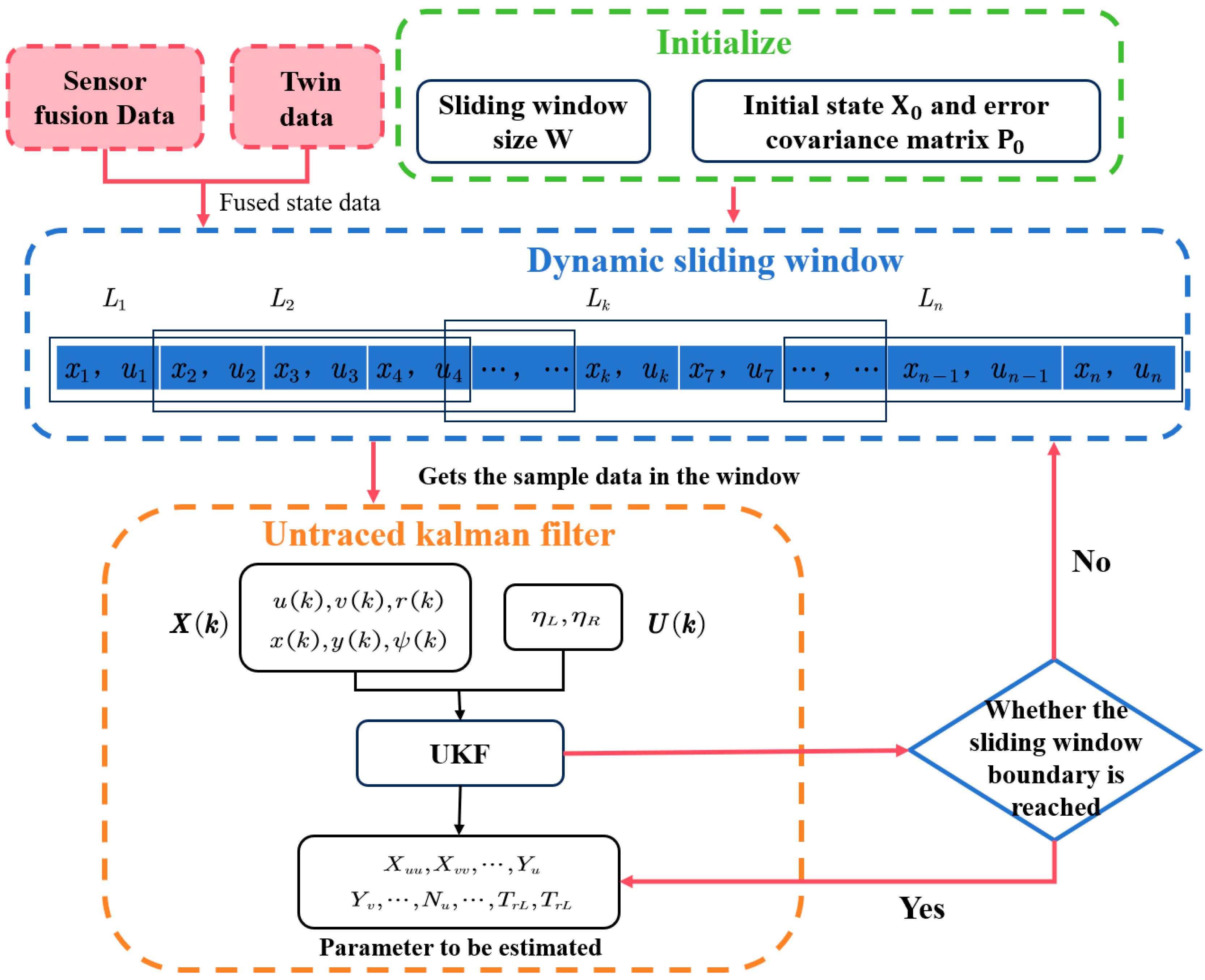
Therefore, this paper proposed an unmanned boat navigation attitude prediction framework that integrates the improved UKF algorithm and digital twin technology. As shown in Figure 1, the method achieves high-precision dynamic mapping between virtual and real environments through a closed-loop feedback mechanism of the digital twin and filtering algorithms. The core innovations of this paper can be summarized as the following three key contributions:

• Development of a digital twin model (DT-Model) for the USV: A high-fidelity modeling approach for complex marine environments is proposed using digital twin technology. This method integrates the kinematics, dynamics, and control models of the USV, as well as environmental disturbance factors, to establish a fully parameterized digital twin model.
• Proposal of a Virtual–Real Synchronization Adjustment Mechanism based on the improved UKF algorithm: Multi-source sensor fusion data including GPS and IMU (Inertial Measurement Unit) data are combined with the improved UKF algorithm to perform real-time attitude estimation and model updates. A filter optimization strategy based on dynamic adjustment of the noise covariance matrix is proposed to enable dynamic updates of the digital twin model.
• By combining twin data with actual measurement data, a time-domain rolling prediction based on the calibrated model is realized: Using the calibrated digital twin model, a navigation attitude prediction model is developed, and the sliding time window technique is used to perform rolling predictions of future navigation attitudes.

The structure of this paper is organized as follows: Section 2 constructs a high-fidelity digital twin model of the unmanned boat from multiple perspectives; Section 3 details the prediction twin model and the improved UKF algorithm for dynamically updating the twin model parameters; Section 4 verifies the effectiveness of the prediction method through comparative experiments and provides analysis; Section 5 discusses the technical limitations and future research directions, culminating in the research conclusions.

2. Problem Description

To accurately predict the navigation attitude of unmanned surface vessels (USVs), digital twin technology offers an effective solution. The development of a digital twin model for the USV is a key component of this approach. Based on the mechanistic model of the USV, a corresponding digital twin model is constructed and dynamically updated using real-time sensor data. This section presents the digital twin method, the mathematical modeling of the USV, and the process of constructing the digital twin model.

2.1. Digital Twin Method

Digital twin technology, originally developed in the field of industrial manufacturing, has been increasingly applied to the modeling and operational management of complex engineering systems. Its core concept involves constructing a virtual model that closely mirrors the physical system, continuously updated using real-time sensor data. In this work, a hybrid modeling approach is adopted for the digital twin, combining physics-based models with data-driven methods. This integration allows the digital twin to leverage the interpretability and generalization of physical models along with the adaptability and predictive capabilities of data-driven techniques. Through this hybrid model, the digital twin enables continuous monitoring, accurate reconstruction, and forward-looking prediction of the system’s operational state.

Beyond serving as a modeling tool for unmanned surface vessel (USV) navigation systems, digital twins also function as key components for real-time state estimation and short-term attitude prediction. In this study, the digital twin method is defined as an integrated technical framework that combines high-fidelity modeling, real-time sensing, data fusion, and predictive analytics. Specifically, real-time sensor data collected from the physical USV is transmitted to the digital twin model, which is iteratively optimized through system identification algorithms to achieve dynamic synchronization between the physical entity and its virtual representation. This process significantly enhances the model’s responsiveness and predictive capability, thereby providing robust technical support for USV navigation and control.

Figure 2 illustrates the architecture of the digital twin USV. This architecture supports bidirectional communication between the physical USV and its virtual model deployed on the digital twin platform, enabling real-time data exchange and model updates. The digital twin platform serves as a comprehensive software environment for the creation, deployment, and management of digital twins. It provides a centralized repository for storing and organizing multi-source sensor data. Upon receiving sensor data, the virtual USV within the platform utilizes an improved Unscented Kalman Filter (UKF) algorithm (as detailed in Section 3) to reconstruct the vessel’s navigation attitude and estimate related dynamic parameters. Based on this, a prediction model using first-order differences is established to forecast the future navigation attitude of the physical USV, thereby enabling intelligent, data-driven control strategies.

2.2. Construction of USV Mathematical Model

The mechanistic model can accurately capture the motion process of the unmanned surface vehicle (USV) and its interactions with the environment, ensuring that the prediction results align with physical laws and real-world operational conditions. Compared to statistical or machine learning models, mechanistic models offer higher accuracy and interpretability in modeling dynamic systems. Therefore, this study chooses to construct a mathematical model based on the mechanistic model of the USV, which includes the development of the kinematic model, dynamic model, control model, environmental disturbance model, and three-dimensional geometric model of the USV.

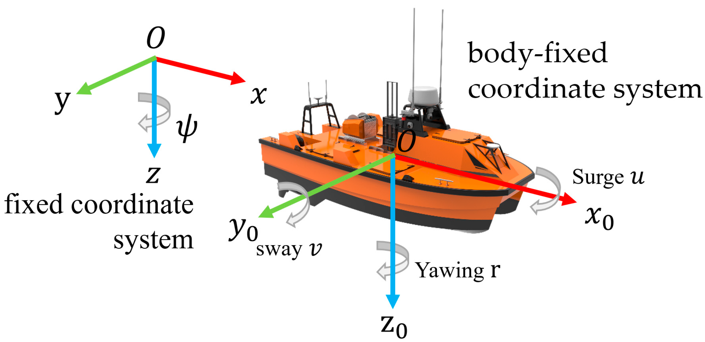
2.2.1. Kinematic Model

The kinematic model of the unmanned boat is described using the six-degree-of freedom (6-DOF) motion equations, as shown in Figure 3. In this paper, the right-handed coordinate system is used. The fixed coordinate system is used to describe the position of the unmanned boat on the water surface, while the body-fixed coordinate system is used to describe its navigation attitude.

In the fixed coordinate system, $\left(x,y,z\right)$ represents the position vector of the unmanned boat, and $\left(\phi ,\theta ,\psi \right)$ represents the attitude vector of the unmanned boat. In the body-fixed coordinate system, $\overrightarrow{V}={\left(u,v,w\right)}^T$ represents the velocity vector of the unmanned boat, and $\overrightarrow{\Omega }={\left(p,q,r\right)}^T$ represents the angular velocity vector.

The transformation between the two coordinate systems is achieved through a rotation matrix, where the coordinate transformation is defined using Euler angles. The transformation matrix is given by $R=R_z\left(\psi \right)R_y\left(\theta \right)R_x\left(\phi \right)$, where $R_x\left(\phi \right)$, $R_y\left(\theta \right)$, and $R_z\left(\psi \right)$ are the rotation matrices about the x, y, and z axes, respectively.

$$R_x\left(\phi \right)=\left[\begin{array}{ccc}1& 0& 0\\ 0& \cos \phi & -\sin \phi \\ 0& \sin \phi & \cos \phi \end{array}\right], R_y\left(\theta \right)=\left[\begin{array}{ccc}\cos \theta & 0& \sin \theta \\ 0& 1& 0\\ \sin \theta & 0& \cos \theta \end{array}\right], R_z\left(\psi \right)=\left[\begin{array}{ccc}\cos \psi & -\sin \psi & 0\\ \sin \psi & \cos \psi & 0\\ 0& 0& 1\end{array}\right],$$

(1)

Specifically, Equation (1) defines the transformation from body-fixed velocity components $\left(u,v,w\right)$ to position derivatives $\left(\dot{x},\dot{y},\dot{z}\right)$ in the earth-fixed frame, expressed as

$$\left[\begin{array}{c}\dot{x}\\ \dot{y}\\ \dot{z}\end{array}\right]=R\left[\begin{array}{c}u\\ v\\ w\end{array}\right],$$

(2)

Equation (2) describes the transformation from body-fixed angular velocity components $\left(p,q,r\right)$ to the time derivatives of Euler angles $\left(\dot{\phi },\dot{\theta },\dot{\psi }\right)$, given by

$$\left[\begin{array}{c}\dot{\phi }\\ \dot{\theta }\\ \dot{\psi }\end{array}\right]=\left[\begin{array}{ccc}1& \sin \phi \tan \theta & \cos \phi \tan \theta \\ 0& \cos \phi & -\sin \phi \\ 0& \sin \phi \sec \theta & \cos \phi \sec \theta \end{array}\right]\left[\begin{array}{c}p\\ q\\ r\end{array}\right],$$

(3)

2.2.2. Dynamic Model

The motion of the USV on the sea can be regarded as the motion of a solid body in a fluid, with the external force and external torque acting on it denoted as F and T, respectively.

$$\left\{\begin{array}{c}F={\left[\begin{array}{ccc}X& Y& Z\end{array}\right]}^T,\\ T={\left[\begin{array}{ccc}K& M& N\end{array}\right]}^T\end{array}\right.,$$

(4)

where X, Y, and Z represent the longitudinal force, lateral force, and vertical force acting on the unmanned vessel, while K, M, and N represent the roll moment, pitch moment, and yaw moment, respectively. As shown in the formula, the external force and torque acting on the unmanned vessel are divided into fluid inertial force $F_I$, fluid viscous force $F_H$, propeller thrust $F_P$, wind force $F_W$, and wave force $F_w$. Each of these forces and moments can be decomposed into the forces and moments along each axis.

$$\left\{\begin{array}{c}F=F_I+F_H+F_P+F_W+F_w,\\ T=T_I+T_H+T_P+T_W+T_w\end{array}\right.,$$

(5)

Based on the MMG (Maneuvering Model Group) [26] modular mathematical model for ship maneuvering, the matrix equation describing the six-degree-of-freedom nonlinear motion of the USV is formulated as

$$\left\{\begin{array}{c}\begin{array}{c}m[\dot{u}-vr+wq-x_G(q^2+r^2)+y_G(pq-\dot{r})+z_G(pr+\dot{q}\left)\right]=X_I+X_H+X_P+X_W+X_w\\ m[\dot{v}-wp+ur-y_G(p^2+r^2)+z_G(qr-\dot{p})+x_G(qp+\dot{r}\left)\right]=Y_I+Y_H+Y_P+Y_W+Y_w\\ m[\dot{w}-uq+vp-z_G(p^2+q^2)+x_G(rp-\dot{q})+y_G(rq+\dot{p}\left)\right]=Z_I+Z_H+Z_P+Z_W+Z_w\end{array}\\ \begin{array}{c}{I}_{xx}\dot{p}-I_{xy}\dot{q}-I_{xx}\dot{r}+(I_{zz}r-I_{xx}p-I_{zy}q)q+(I_{yx}p+I_{zx}r-I_{yy}q)r\\ +m\left[y_G\right(w+vp-uq)-z_G(\dot{v}+ur-wp\left)\right]=K_I+K_H+K_P+K_W+K_w\\ I_{xx}\dot{q}-I_{xy}\dot{p}-I_{xz}\dot{r}+(I_{xx}p-I_{xy}q-I_{xz}r)r+(I_{xz}p+I_{zy}q-I_{zz}r)p\\ +m\left[z_G\right(u+wq-vr)-x_G(\dot{v}q+vp-uq\left)\right]=M_I+M_H+M_P+M_W+M_w\\ I_{zz}\dot{r}-I_{xy}\dot{q}-I_{xz}\dot{p}+(I_{yy}q-I_{xy}p-I_{zz}r)p+(I_{xz}r+I_{xz}q-I_{xx}p)q\\ +m\left[x_G\right(\dot{v}+ur-wp)-y_G(\dot{u}+wq-vr\left)\right]=N_I+N_H+N_P+N_W+N_w\end{array}\end{array}\right.,$$

(6)

where $m$ represents the mass of the USV, and $I_{xx}$, $I_{yy}$, and $I_{zz}$ are the moments of inertia about the x, y, and z axes, respectively. $I_{xy}$, $I_{xz}$, and $I_{yz}$ represent the inertia coupling terms of the USV with respect to different axes. $x_G$, $y_G$, and $z_G$ denote the offsets of the center of mass relative to the reference point.

In this paper, it is assumed that point O coincides with the position of the center of gravity (G), and that the position of the center of gravity does not shift during navigation. It is also assumed that the unmanned surface vessel (USV) is symmetric about the xz plane, and that its heave, pitch, and roll motions can be neglected [27]. The research object in this study is a 7.5 m long unmanned surface vessel, and only a three-degree-of-freedom maneuvering mathematical model is sufficient to meet the experimental requirements. Based on these assumptions, the dynamics equation of the USV in three degrees of freedom is simplified from Equation (6) and expressed as Equation (7):

$$\left\{\begin{array}{c}m\left(\dot{u}-vr\right)=X_I+X_H+X_P+X_W+X_w\\ m\left(\dot{v}+ur\right)=Y_I+Y_H+Y_P+Y_W+Y_w\\ I_{zz}\dot{r}=N_I+N_H+N_P+N_W+N_w\end{array}\right.,$$

(7)

When the unmanned surface vessel (USV) accelerates or decelerates in a fluid, the inertial reaction force from the fluid affects the USV’s navigation attitude. This force is known as the fluid inertia force. According to the literature [28], its expression is as follows:

$$\left\{\begin{array}{c}{X}_I=-m_x\dot{u}+m_y\nu r\\ Y_I=-m_y\dot{v}-m_{x}ur\\ N_I=-J_z\dot{r}\end{array}\right.,$$

(8)

where $m_x$, $m_y$, and $J_z$ are the added mass and added moment of inertia coefficients of the USV.

The presence of viscous forces causes relative resistance between fluid layers moving at different velocities, thereby affecting the motion of the unmanned surface vehicle (USV). The fluid viscous force acting on the USV is referenced in [29] as follows, with $X_{uu}$, …, $N_{vr}$ being the viscous force coefficients:

$$\left\{\begin{array}{c}{X}_H=X_{uu}{u}^2+X_{vv}{v}^2+X_{vr}vr+X_{rr}{r}^2\\ Y_H=Y_{v}v+Y_{r}r+Y_{v\left|v\right|}v\mid v\mid +Y_{v\left|v\right|}v\mid r\mid +Y_{r\left|v\right|}r\mid r\mid \\ N_H=N_{v}v+N_{r}r+N_{r\left|r\right|}r\mid r\mid +N_{vvr}{v}^{2}r+N_{vrr}v{r}^2\end{array}\right.,$$

(9)

The subject of this study is a twin-propeller unmanned surface vehicle (USV). The thrust it experiences is described by Equation (10):

$$\left\{\begin{array}{c}{X}_p=T_{L}cos\left({\delta }_L\right)+T_{R}cos\left({\delta }_R\right)\\ Y_p=T_{L}sin\left({\delta }_L\right)+T_{R}sin\left({\delta }_R\right)\\ N_p=(T_{L}cos({\delta }_L)-T_{R}cos({\delta }_R\left)\right)\cdot 0.5\cdot L_{LR}-Y_P\cdot L_{OP}\end{array}\right.,$$

(10)

where $X_p$ represents the total thrust in the X-direction on the unmanned surface vehicle, synthesized from the thrust components of the two propellers. $Y_p$ denotes the total thrust in the Y-direction, which primarily affects the lateral motion of the vessel. $N_p$ describes the yawing moment caused by the unbalanced thrust produced by the two propellers; if the two propellers generate different thrusts (i.e., $T_L\ne T_R$), a moment about the Z-axis is produced, leading to yawing of the vessel. $L_{LR}$ is the distance between the left and right propellers, and $L_{OP}$ is the longitudinal coordinate of the propellers.

2.2.3. Control Model

The rudder angle of the unmanned boat is controlled through a deflection indicator control model, where the rate of change of the rudder angle $\dot{\eta }$ is adjusted based on the deviation between the desired rudder angle ${\eta }_E$ and the actual rudder angle.

$$\dot{\eta }=\left\{\begin{array}{cc}sgn\left({\eta }_E\right)k_{\eta }& \eta <\left|{\eta }_E\right|\\ 0& \eta \ge \left|{\eta }_E\right|\end{array}\right.,$$

(11)

where ${\eta }_E$ represents the desired rudder angle (in degrees), i.e., the target rudder angle to be achieved by the control system; $k_{\mathsf{\eta }}$ is the inertia slope in the rudder angle response process, describing the rate at which the rudder angle changes over time. $sgn\left({\mathsf{\eta }}_E\right)$ is the sign function, indicating the direction of rudder angle adjustment (positive or negative); when $\left|\mathsf{\eta }\right|<\left|{\mathsf{\eta }}_E\right|$, the rudder angle is adjusted according to the sign function; when $\left|\eta \right|\ge \left|{\eta }_E\right|$, the rudder angle no longer changes, indicating that the rudder angle has reached the desired value.

2.2.4. Environmental Disturbance Model

During actual navigation, an unmanned surface vehicle (USV) may encounter environmental disturbances such as wind and waves, which can cause deviations from its intended path. Therefore, the influence of these disturbances on the USV during its movement is considered. This paper models the forces exerted by wind and waves on the USV. The calculation of wind forces is primarily based on aerodynamic principles [30]. The average wind force and the moments generated by the wind are given in Equation (12):

$$\left\{\begin{array}{c}{X}_W=0.5{\rho }_a{V}_{wR}^2{A}_T{C}_{wx}\left({\alpha }_w\right)\\ Y_W=0.5{\rho }_a{V}_{wR}^2{A}_L{C}_{wy}\left({\alpha }_w\right)\\ N_{\mathrm{W}}=0.5{\rho }_a{V}_{wR}^2{A}_{L}L{C}_{wn}\left({\alpha }_w\right)\end{array}\right.,$$

(12)

The wind force and wind moment coefficients are estimated using the Blendermann empirical formula [31], as shown in Formula (13):

$$\left\{\begin{array}{cc}{C}_{Xwi}& =-C_{D1}{\displaystyle \frac{A_L}{A_T}}{\displaystyle \frac{\mathit{cos}\left({\alpha }_w\right)}{1-\frac{{\delta }_w}{2}(1-\frac{C_{D1}}{C_{Dt}}){sin}^2\left(2{\alpha }_w\right)}}\\ C_{Ywi}& =C_{Dt}{\displaystyle \frac{\mathit{sin}\left({\alpha }_w\right)}{1-\frac{{\delta }_w}{2}(1-\frac{C_{D1}}{C_{Dt}}){sin}^2\left(2{\alpha }_w\right)}}\\ C_{Nwi}& =[{\displaystyle \frac{s_L}{L}}-0.18({\alpha }_w-{\displaystyle \frac{\pi }{2}}\left)\right]\cdot C_{Y_{wi}}\end{array}\right.,$$

(13)

Marine environments are characterized by complex wave patterns, typically irregular waves. This paper assumes that the waves are long-crested, and according to wave theory [32], the wave height at a given point on the sea surface is represented as follows:

$$\zeta (t)={\sum }_{i=1}^{\infty }{\zeta }_{ai}cos(k_i\xi cos\mu +k_i\eta sin\mu -{\omega }_{i}t+{\epsilon }_i),$$

(14)

where ${\mathsf{\zeta }}_{ai}$, $k_i$, ${\mathsf{\omega }}_i$, and ${\mathsf{\epsilon }}_i$ are the amplitude, wave number, angular frequency, and initial phase of the i-th harmonic wave, respectively.

In this paper, the PM (Pierson–Moskowitz) wave spectrum [33] is fitted using wind and wave data as shown in Equation (15):

$$S\left(w\right)=\alpha {\displaystyle \frac{g^2}{w^5}}exp\left(-\beta {\left({\displaystyle \frac{w}{w_0}}\right)}^4\right),$$

(15)

where $\alpha =8.1\times {10}^{-3}$, $\beta =0.74$, $w_0=g/U_{19.5}$, and $U_{19.5}$ is the wind speed at 19.5 m above the water surface. It is typically assumed that $U_{19.5}=1.026 U$, where U is the wind speed at sea level.

The free-surface variance is given by the following:

$${\overline{n}}^2={\int }_0^{\infty }S\left(w\right)dw=0.00274{\displaystyle \frac{U^4}{g}},$$

(16)

The integration is taken over the frequency spectrum from zero to infinity, as the total wave energy is distributed over all frequencies.

The significant wave height $H_s$ can be estimated as $4n$. Substituting this expression into Equation (15), the wave spectrum can be written in terms of the significant wave height:

$$S_{\zeta }(\omega )={\displaystyle \frac{8.1\times {10}^{-3}{g}^2}{{\omega }^5}}exp(-0.031{({\displaystyle \frac{g}{{\omega }^2{H}_s}})}^2),$$

(17)

this equation describes the energy distribution of the waves, where the energy is a function of both the frequency and the significant wave height $H_s$.

The equations for the wave forces and moments acting on the USV are formulated based on reference [34] as follows:

$$\left\{\begin{array}{c}{X}_w=0.5\rho Lcos\chi \sum _{i=1}^m{c}_{Xw}\left({\lambda }_i\right){\zeta }_{ai}^2\\ Y_w=0.5\rho Lsin\chi \sum _{i=1}^m{C}_{Yw}\left({\lambda }_i\right){\zeta }_{ai}^2\\ N_w=0.5\rho Lsin\chi \sum _{i=1}^m{C}_{Nw}\left({\lambda }_i\right){\zeta }_{ai}^2\end{array}\right.,$$

(18)

Here, $C_{Xw}$, $C_{Yw}$ and $C_{Nw}$ represent the wave force and moment coefficients, which are estimated based on Equation (18) from reference [35]:

$$\left\{\begin{array}{c}{C}_{Xw}=0.05-0.2\left({\displaystyle \frac{\lambda }{L}}\right)+0.75{\left({\displaystyle \frac{\lambda }{L}}\right)}^2-0.51{\left({\displaystyle \frac{\lambda }{L}}\right)}^3\\ C_{Yw}=0.46+6.83\left({\displaystyle \frac{\lambda }{L}}\right)-15.65{\left({\displaystyle \frac{\lambda }{L}}\right)}^2+8.44{\left({\displaystyle \frac{\lambda }{L}}\right)}^3\\ C_{Nw}=-0.11+0.68\left({\displaystyle \frac{\lambda }{L}}\right)-0.79{\left({\displaystyle \frac{\lambda }{L}}\right)}^2+0.21{\left({\displaystyle \frac{\lambda }{L}}\right)}^3\end{array}\right.,$$

(19)

2.2.5. 3D Geometric Model

The three-dimensional (3D) geometric model of the USV digital twin serves as an accurate digital representation of its physical structure, encompassing the hull shape, internal framework, and key components such as thrusters, rudders, and sensors. This model must precisely reflect the USV’s dimensions, mass distribution, and inertial properties while being compatible with computational fluid dynamics (CFD) and structural simulation tools to facilitate environmental interaction modeling, motion behavior analysis, and dynamic response simulations. As shown in Figure 4, this study utilizes 3Ds Max (https://www.autodesk.com/products/3ds-max/overview, accessed on 28 April 2025) to construct and assemble 3D models of various USV components, forming a complete and detailed USV model. The created model is then exported in .fbx format and imported into the UE4-based digital twin platform. This ensures that the virtual USV model is fully consistent with its physical counterpart, allowing for accurate simulation of hydrodynamic forces and motion behavior in a virtual environment.

2.3. Construction of USV Digital Twin Model

There are several approaches to constructing a twin model, including mechanistic twin models built based on various physical and mathematical analysis methods, nonlinear mapping twin models constructed using neural networks, and twin models based on AR (Autoregressive) model structures [36]. Mechanistic modeling, grounded in physical laws, offers high interpretability and low data dependency. It can accurately describe the dynamics of unmanned surface vehicles (USVs) and is well suited for scenarios with known mechanisms and stable environments. Moreover, mechanistic models exhibit good generalization ability, making them applicable across various scenarios with stability. In contrast, data-driven modeling, while adaptable to complex environments, relies heavily on large volumes of high-quality data and lacks interpretability. It is often less effective at predicting in unknown scenarios. AR models are restricted to linear systems, making them less capable of handling complex nonlinear systems, and their long-term prediction errors are prone to accumulation. Overall, mechanistic modeling holds an advantage in terms of accuracy and reliability, making it particularly beneficial for environments where the underlying system behavior is well understood.

Building upon the mathematical model of the USV established in Section 2.2, the corresponding digital twin model is developed. Based on the previously constructed framework, the USV digital twin model is formulated as shown in Equation (20):

$$\left\{\begin{array}{l}\dot{u}=X_{uu}{u}^2+X_{vv}{v}^2+X_{vr}vr+X_{rr}{r}^2+T_{uL}{n}_L^2\cos {\delta }_p+T_{uR}{n}_R^2\cos {\delta }_s\hfill \\ \dot{\nu }=Y_{u}u+Y_v\nu +Y_{r}r+Y_{v\left|v\right|}\nu \left|\nu \right|+Y_{v\left|r\right|}\nu \left|r\right|+\hfill \\ \hspace{1em} Y_{r\left|r\right|}r\left|r\right|+Y_{ur}ur+T_{vL}{n}_L^2\sin {\delta }_p+T_{vR}{n}_R^2(k)\sin {\delta }_S\hfill \\ \dot{r}=N_{u}u+N_{v}v+N_{r}r+N_{r\left|r\right|}r\left|r\right|+N_{vvr}{v}^{2}r+N_{vrr}\nu r^2\hfill \\ \hspace{1em} +T_{rL}{n}_L^2\nu \sin {\delta }_p+T_{rR}{n}_R^2\nu \sin {\delta }_s\hfill \\ \dot{x}=u\cos \psi -\nu \sin \psi \hfill \\ \dot{y}=u\sin \psi +\nu \cos \psi \hfill \\ \dot{\psi }=r\hfill \end{array}\right.,$$

(20)

Here, the dimensioned viscous force coefficient and propeller thrust coefficient are selected as the identification targets, forming the parameter vector ${\mathsf{\xi }}_i$ to be optimized, as shown in Equation (21):

$$\left\{\begin{array}{l}{\mathit{\xi }}_{\mathit{u}}=\left[X_{uu}\hspace{0.33em}{X}_{vv}\hspace{0.33em}{X}_{vr}\hspace{0.33em}{X}_{rr}\hspace{0.33em}{T}_{uL}\hspace{0.33em}{T}_{uR}\right]\hfill \\ {\mathit{\xi }}_{\mathit{v}}=\left[Y_u\hspace{0.33em}{Y}_v\hspace{0.33em}{Y}_r\hspace{0.33em}{Y}_{v\left|v\right|}\hspace{0.33em}{Y}_{v\left|r\right|}\hspace{0.33em}{Y}_{r\left|r\right|}\hspace{0.33em}{Y}_{ur}\hspace{0.33em}{T}_{vL}\hspace{0.33em}{T}_{vR}\right]\hfill \\ {\mathit{\xi }}_{\mathit{r}}=\left[N_u\hspace{0.33em}{N}_v\hspace{0.33em}{N}_r\hspace{0.33em}{N}_{v\left|v\right|}\hspace{0.33em}{N}_{v\left|r\right|}\hspace{0.33em}{N}_{r\left|r\right|}\hspace{0.33em}{N}_{vvr}\hspace{0.33em}{N}_{vrr}\hspace{0.33em}{T}_{rL}\hspace{0.33em}{T}_{rR}\right]\hfill \end{array}\right.\hspace{0.33em},$$

(21)

Define ${\mathsf{\phi }}_i$ as the input matrix, as shown in Equation (22):

$$\left\{\begin{array}{l}{\mathsf{\phi }}_u=\left[u^2\hspace{0.33em}{v}^2\hspace{0.33em}{r}^2\hspace{0.33em}vr\hspace{0.33em}{n}_L^2\cos {\delta }_P\hspace{0.33em}{n}_R^2\cos {\delta }_S\right]\hfill \\ {\mathsf{\phi }}_v=\left[u\hspace{0.33em}v\hspace{0.33em}r\hspace{0.33em}v\left|v\right|\hspace{0.33em}v\left|r\right|\hspace{0.33em}r\left|r\right|\hspace{0.33em}ur\hspace{0.33em}{n}_L^2\cos {\delta }_P\hspace{0.33em}{n}_R^2\cos {\delta }_S\right]\hfill \\ {\mathsf{\phi }}_r=\left[u\hspace{0.33em}v\hspace{0.33em}r\hspace{0.33em}v\left|v\right|\hspace{0.33em}v\left|r\right|\hspace{0.33em}r\left|r\right|\hspace{0.33em}{v}^{2}r\hspace{0.33em}v{r}^2\hspace{0.33em}{n}_L^2\cos {\delta }_P\hspace{0.33em}{n}_R^2\cos {\delta }_S\right]\hfill \end{array}\right.,$$

(22)

Thus, the digital twin model can be expressed in the following form, where $Z_i$ represents the output matrix:

$${\mathit{Z}}_{\mathit{i}}={\mathit{\phi }}_{\mathit{i}}{\mathit{\xi }}_{\mathit{i}}^{\mathit{T}}+{\epsilon }_i, i=u,v,r,$$

(23)

3. USV Navigation Attitude Prediction Method

A mechanistic-based twin model was established in Section 2 to support state estimation and dynamic prediction of the USV. Building on this, this section develops a digital twin prediction model using time-series analysis, integrating the improved Unscented Kalman Filter algorithm to identify key parameters, resulting in a more accurate model for predicting the USV’s future navigation states. The key steps in parameter identification include three parts: the establishment of the USV model, the construction of the identification model, and the design of the identification algorithm. Section 2 discusses the model construction, while this section focuses on the development of the identification model and the identification algorithm.

3.1. USV Three-Degree-of-Freedom Prediction Twin Model

First-order differences are a method used in time-series analysis to measure the change between two adjacent data points, which helps reveal the trend of data variations [37]. This paper constructs a three-degree-of-freedom motion prediction model for the unmanned boat based on first-order differences to forecast its motion. The formula for first-order differences is given by Equation (23):

$$\dot{t}\left(k\right)={\displaystyle \frac{t\left(k+1\right)=t\left(k\right)}{h}},$$

(24)

Based on the above equation, the constructed digital twin prediction model is formulated as Equation (25). The attitude prediction of the unmanned surface vehicle (USV) is then carried out according to Equation (25):

$$x\left(k+1\right)=x\left(k\right)+f\left(x\left(k\right),u\left(k\right)\right)\cdot h,$$

(25)

Here, ${u\left(k\right)=\left[{\eta }_L\left(k\right),{\eta }_R\left(k\right),{\delta }_p\left(k\right),{\delta }_s\left(k\right)\right]}^T$ is the control input vector (left/right propeller speeds and rudder angles), $x\left(k\right)={\left[u\left(k\right),v\left(k\right),r\left(k\right),x\left(k\right),y\left(k\right),\mathsf{\psi }\left(k\right)\right]}^T$ represents the navigation attitude of the USV at time k, obtained through sensor fusion. $h$ is the integration step size, and $f\left(·\right)$ is a nonlinear function that encodes the dynamic behavior of the system.

The function $f\left(x,u\right)$ is composed of the following six elements, derived from the original differential equations:

$$f=\left[\begin{array}{c}{X}_{uu}{u}^2+X_{vv}{v}^2+X_{vr}vr+X_{rr}{r}^2+T_{uL}{n}_L^{2}cos\left({\delta }_p\right)+T_{uR}{n}_R^{2}cos\left({\delta }_s\right)\\ Y_{u}u+Y_{v}v+Y_{r}r+Y_{v\left|\nu \right|}v\left|\nu \right|+Y_{v\left|r\right|}v\left|r\right|+Y_{r\left|r\right|}r\left|r\right|+{Y_{ur}ur+T}_{vL}{n}_L^{2}sin\left({\delta }_p\right)+T_{vR}{n}_R^{2}sin\left({\delta }_s\right)\\ N_{u}u+N_{v}v+N_{r}r+N_{r\left|r\right|}u\left|r\right|+N_{vrr}v{r}^2+N_{vv\left|r\right|}{v}^{2}r+T_{rL}{n}_L^{2}sin\left({\delta }_p\right)+T_{rR}{n}_R^{2}sin\left({\delta }_s\right)\\ ucos\left(\psi \right)-vsin\left(\psi \right)\\ usin\left(\psi \right)+vcos\left(\psi \right)\\ r\end{array}\right],$$

(26)

Based on Equation (26), the future rudder angle prediction is derived as follows:

$${\eta }_i(k+1)=\left\{\begin{array}{cc}{\eta }_i\left(k\right)+\mathrm{sgn}\left({\eta }_E\right)k_{\eta }h& {\eta }_i\left(k\right)<\left|{\eta }_E\right|\\ {\eta }_E& {\eta }_i\left(k\right)\ge \left|{\eta }_E\right|\end{array}i=L,R\right.,$$

(27)

3.2. USV Prediction Digital Twin Model Identification Method

3.2.1. UKF Parameter Identification

The UKF is an attitude estimation algorithm suitable for nonlinear systems. It uses a set of carefully selected sample points (called Sigma points) to approximate the statistical characteristics of nonlinear functions, thereby avoiding the errors introduced during the linearization process of the EKF (Extended Kalman Filter) through Taylor series expansion [38]. This results in higher estimation accuracy and stability. To identify the parameters of the twin model, this paper introduces the Unscented Kalman Filter algorithm into the parameter identification of the unmanned boat motion twin model, where the model parameters are treated as variables.

For an n-dimensional nonlinear system, its attitude–space model is as follows:

$$\left\{\begin{array}{c}{\mathit{X}}_k=f({\mathit{X}}_{k-1},{\mathit{U}}_k)+w_k,\\ {\mathit{Z}}_k=h\left({\mathit{X}}_k\right)+v_k\end{array}\right.,$$

(28)

where ${\mathit{X}}_k$ is the system’s attitude vector at time k; $f$ is the state transition function, which depends on the previous attitude ${\mathit{X}}_{k-1}$ and the current control input ${\mathit{U}}_k$; $w_k$ is the process noise following a Gaussian distribution, typically assumed to be zero mean with variance ${\mathit{Q}}_k$ (white noise); ${\mathit{Z}}_k$ is the system’s observation vector at time k; $h$ is the system observation function, typically nonlinear; $v_k$ is the observation noise, usually assumed to be zero mean with variance ${\mathit{R}}_k$ (white noise). The steps of the UKF algorithm can be described as follows:

To capture the mean and covariance of the prior state distribution, a set of $2n+1$ sigma points is generated from the current estimated state ${\mathit{X}}_{k-|k-1}$ and error covariance $P_{k-|k-1}$:

$$\left\{\begin{array}{l}{\mathit{X}}_{0,k-1|k-1}={\widehat{\mathit{X}}}_{k-1|k-1},\\ {\mathit{X}}_{i,k-1|k-1}={\widehat{\mathit{X}}}_{k-1|k-1}\pm \sqrt{\left(n+k\right)P_{k-1|k-1}},i=\mathrm{1,2}\dots 2n\end{array}\right.,$$

(29)

where $i=\mathrm{1,2},\dots ,n$, $\lambda ={\alpha }^2\left(n+k\right)-n$, and $\alpha$, $k$ are scaling parameters. The square root is typically computed via Cholesky decomposition.

State estimation prediction and error covariance matrix prediction:

$$\left\{\begin{array}{c}{\mathit{X}}_{k|k-1},{\mathit{P}}_{k|k-1}^{\prime }=UT({\mathit{X}}_{k-1},{\mathit{P}}_{k-1},f),\\ {\mathit{P}}_{k|k-1}={\mathit{P}}_{k|k-1}^{\prime }+{\mathit{Q}}_k\end{array}\right.,$$

(30)

Filter gain:

$$\left\{\begin{array}{c}{\mathit{Z}}_{k|k-1},{\mathit{P}}_{zz}^{\prime }=UT({\mathit{X}}_{k|k-1},{\mathit{P}}_{k|k-1},h),\\ {\mathit{P}}_{zz}={\mathit{P}}_{zz}^{\prime }+{\mathit{R}}_k,\\ {\mathit{P}}_{xz}=U{T}_c({\mathit{X}}_{k|k-1},{\mathit{P}}_{k|k-1},f,h),\\ G_k={\mathit{P}}_{xz}{\mathit{P}}_{zz}^{-1}\end{array}\right.,$$

(31)

State estimation update:

$${\mathit{X}}_k={\mathit{X}}_{k|k-1}+G_k({\mathit{Z}}_k-{\mathit{Z}}_{k|k-1}),$$

(32)

Error covariance matrix update:

$${\mathit{P}}_k={\mathit{P}}_{k|k-1}-G_k{\mathit{P}}_{zz}{\mathit{G}}_k^T,$$

(33)

To enable online identification of model parameters, the parameters to be identified are incorporated into the attitude vector, thereby expanding the attitude space. For instance, model parameters such as damping coefficients and added mass are treated as extended attitudes:

$${\mathit{X}}_k^{\prime }=\left[\begin{array}{c}{\mathit{X}}_k\\ {\mathit{\xi }}_k\end{array}\right],$$

(34)

where ${\mathit{\xi }}_k$ is the vector of model parameters. During the UKF process, the parameters are estimated along with the attitude, enabling online identification.

3.2.2. Online Parameter Identification Method Based on Dynamic Sliding Window

Although the UKF has advantages in handling nonlinear systems, when used alone to identify the twin model parameters, attitude estimation typically relies on current observation data and recent attitudes. This makes the estimation vulnerable to transient errors, such as those caused by noise or sudden external disturbances, which can significantly impact the parameter estimates [39]. In dynamic environments, relying on a single observation data point can lead to instability in parameter estimation, affecting identification accuracy and making it difficult to estimate model parameters in a timely and precise manner.

To address these issues, this paper introduces an online parameter identification method based on a dynamic sliding window. The length of the window is dynamically adjusted based on changes in the system’s attitude and error characteristics, allowing the window to adaptively shrink or expand over time and in response to system attitude changes, thereby enabling more accurate parameter identification. The schematic of the dynamic sliding window is shown in Figure 5.

The core of the dynamic sliding window is the definition of an adjustment mechanism that determines the window’s dynamic changes based on the system’s attitude variations and error characteristics [15]. This paper defines the total length $W$ of the dynamic sliding window as consisting of a base window $w$ and an adaptive adjustment window $∆w\left(r\right)$:

$$W=w+\mathsf{∆}w\left(r\right),$$

(35)

where $w$ is the fixed portion of the window length, determined by the unmanned boat’s dynamic response time constant (e.g., $w=15$ corresponds to 0.75 s of historical data with a sampling frequency of 20 Hz); $∆w\left(r\right)$ is the dynamically adjusted portion, whose size is determined by the characteristics of the attitude data and fluctuations in prediction errors.

This paper adopts a periodic adaptive adjustment strategy to dynamically adjust the size of the sliding window $W$. The specific adjustment rules are as follows:

Setting the adjustment period. The base period $T_0=10 \mathrm{s}$ is determined based on the dominant period of the wave spectrum (3–15 s) and the unmanned boat’s control response time. The adjustment period is then modified based on the real-time feedback of the UKF innovation covariance $P_k$:

$$T=T_0\cdot {(1+{\displaystyle \frac{\mathrm{tr}\left(P_k\right)}{P_{max}}})}^{-1},$$

(36)

where $P_{max}$ is the upper limit of the innovation covariance (e.g., $P_{max}={1.5}^2$ corresponding to the 3σ boundary). When the filtering error increases, the adjustment period is shortened.

Calculating the mean fluctuation of marine environmental parameters in the window: The fluctuation $V_r^{env}$ within the window is calculated by combining wave height $H_s$ and wind speed $V_w$:

$$V_r^{env}={\displaystyle \frac{1}{3}}({\displaystyle \frac{\sigma \left(H_s\right)}{{\overline{H}}_s}}+{\displaystyle \frac{\sigma \left(V_w\right)}{{\overline{V}}_w}}),$$

(37)

Nonlinearity evaluation is performed using the largest Lyapunov exponent. The Lyapunov exponent is used to assess the nonlinearity of the motion attitude. For short time-series data, the maximum Lyapunov exponent is calculated using a small-data method [40]:

$${\lambda }_{max}={\displaystyle \frac{1}{\mathsf{∆}t}}⟨\ln {\displaystyle \frac{\parallel U\left(l+\Delta t\right)-U^{\prime }\left(l+\Delta t\right)\parallel }{\parallel U\left(l\right)-U^{\prime }\left(l\right)\parallel }}⟩,$$

(38)

The nonlinearity index within the window is calculated as

$$S_r^{nonlin}={\displaystyle \frac{1}{W}}{\sum }_{j=k}^{k+W-1}{e}^{{\lambda }_{max}\cdot (t_j-t_k)},$$

(39)

where $S_r^{\mathrm{nonlin}}$ reflects the divergence trend of the data, and $S_r^{\mathrm{nonlin}}>1$ indicates stronger local chaotic characteristics.

Model fusion and weighted optimization are calculated as

$$\Delta w\left(r\right)=⌊w\cdot \left({\gamma }_1\cdot V_r^{env}+{\gamma }_2\cdot S_r^{nonlin}\right)⌋,$$

(40)

Based on Zhuhai sea trial data (wave height levels 1–4), a multiple regression analysis determines the weighting coefficients ${\mathsf{\gamma }}_1=0.6$ and ${\mathsf{\gamma }}_2=0.4$, reflecting the dominant environmental disturbance characteristics. When the IMU lateral acceleration exceeds a threshold $a_y=0.3g$, the system enforces $∆w\left(r\right)=w$, doubling the window length to $2w$, emphasizing the dominance of environmental disturbances. If $V_r^{\mathrm{env}}<0.1$ and $S_r^{\mathrm{nonlin}}<1.2$ hold, then set $∆w\left(r\right)=0$ to save computational power.

At each sampling time, old data $x_k$ is removed, and new real-time data $x_{k+W}$ is added. When $∆w\left(r\right)$ decreases, redundant data at the window’s tail are removed to maintain a total window length $W=w+∆w\left(r\right)$, ensuring the system adapts to dynamic changes. The specific adjustment process is summarized in Algorithm 1.

Algorithm 1 Dynamic Sliding Window Adjustment

$\mathrm{Input}: \mathrm{the} \mathrm{state} \mathrm{observation} \mathrm{variable} (\mathrm{u}, \mathrm{v}, \mathrm{r}, \mathrm{x}, \mathrm{y}, \psi$)

$\mathrm{Output}: \mathrm{Window} \mathrm{size} W$$, \mathrm{the} \mathrm{state} \mathrm{observation} \mathrm{variable} (\mathrm{u}, \mathrm{v}, \mathrm{r}, \mathrm{x}, \mathrm{y}, \psi$)

$1: \mathrm{Initialize} \mathrm{base} \mathrm{window} \mathrm{size} w=15$$, \mathrm{maximum} \mathrm{innovation} \mathrm{covariance} \mathrm{threshold} P_{max}={1.5}^2$$, \mathrm{and} \mathrm{base} \mathrm{adjustment} \mathrm{period} T_0=10$;

$2: \mathrm{Input} \mathrm{current} \mathrm{innovation} \mathrm{covariance} P_k$$, \mathrm{wave} \mathrm{height} H_s$$, \mathrm{wind} \mathrm{speed} V_w$$, \mathrm{and} \mathrm{nonlinearity} \mathrm{index} S_r^{\mathrm{nonlin}}$;

$3: \mathrm{Calculate} \mathrm{environmental} \mathrm{fluctuation} V_r^{\mathrm{env}}$ by

$\hspace{1em}\hspace{1em}\hspace{1em}{V}_r^{\mathrm{env}}=H_s·V_w$;

$4: \mathrm{Estimate} \mathrm{nonlinearity} \mathrm{index} S_r^{\mathrm{nonlin}}$ using the largest Lyapunov exponent;

$5: \mathrm{If} P_k>P_{max}$, then

$6:\hspace{1em}\hspace{1em}\mathrm{Set} \mathrm{adjustment} \mathrm{period} T=T_0/2$;

7: Else

$8:\hspace{1em}\hspace{1em}\mathrm{Set} T=T_0$;

$9:\hspace{1em}\mathrm{Compute} \mathrm{adaptive} \mathrm{window} \mathrm{extension} \Delta w$$\mathrm{by} \mathrm{combining} S_r^{\mathrm{nonlin}}$$\mathrm{and} V_r^{\mathrm{env}}$:

$\hspace{1em}\hspace{1em}\hspace{1em}\hspace{1em}\hspace{1em}∆w=f(S_r^{\mathrm{nonlin}},V_r^{\mathrm{env}})$;

$10: \mathrm{Calculate} \mathrm{total} \mathrm{window} \mathrm{length} W$ as

$\hspace{1em}\hspace{1em}\hspace{1em}\hspace{1em}W=w+∆w\left(r\right)$;

$11: \mathrm{Return} \mathrm{updated} \mathrm{window} \mathrm{size} W$$\mathrm{and} \mathrm{state} \mathrm{observation} \mathrm{variable} (\mathrm{u}, \mathrm{v}, \mathrm{r}, \mathrm{x}, \mathrm{y}, \psi$).

3.2.3. UKF Identification Method Improved by Dynamic Sliding Window

Environmental disturbances and sensor interactions often affect the motion performance of unmanned surface vehicles (USVs), leading to data inaccuracies. To enhance parameter identification accuracy, this study employs sensor data fusion. By combining the strengths of GPS and IMU, the fusion improves attitude estimation robustness. Kalman filtering is used due to its effectiveness in handling noisy measurements [41]. Inspired by [42], a late-stage fusion strategy is adopted, where GPS and IMU data are first independently filtered using Kalman filters. GPS provides global position data, while the IMU offers high-frequency motion information. The resulting attitude estimates are then fused using their respective uncertainty levels.

As illustrated in Figure 6, the diagram presents the sensor fusion process based on GPS and IMU data. GPS and IMU data are used for attitude estimation and prediction separately through Kalman filters, where GPS provides global position information, and IMU offers high-frequency local acceleration and angular velocity data. The fusion module integrates the two sets of attitude estimates to generate a final, more accurate result.

Assuming both filtered signals follow zero mean Gaussian noise with covariances $K_{GPS,k+1}$ and $K_{IMU,k+1}$, the optimal fused attitude is obtained via:

$${\mathsf{\Phi }}_{k+1}=W_{GPS}{\mathsf{\Phi }}_{GPS,k+1}+W_{IMU}{\mathsf{\Phi }}_{IMU,k+1},$$

(41)

with the weights defined as

$$\left\{\begin{array}{c}{W}_{GPS}={\mathrm{K}}_{IMU,k+1}{\left({\mathrm{K}}_{GPS,k+1}+{\mathrm{K}}_{IMU,k+1}\right)}^{-1}\\ W_{IMU}={\mathrm{K}}_{GPS,k+1}{({\mathrm{K}}_{GPS,k+1}+{\mathrm{K}}_{IMU,k+1})}^{-1}\end{array}\right.,$$

(42)

This approach ensures statistically optimal fusion under Gaussian noise, offering improved accuracy and adaptability compared to fixed or empirical weighting methods.

The iterative optimization process of the digital twin model using the dynamic sliding window-improved Unscented Kalman Filter (DSW-UKF) is depicted in Figure 7. First, a sliding window mechanism is employed to dynamically extract twin data and real vessel data from the system. The fused USV data, obtained via Kalman filtering, includes attitude variables (e.g., position, velocity), inputs (control commands), and observations (sensor measurements). These data segments are sequentially processed through the sliding window and fed into the UKF. The UKF utilizes the system model and measurement data to perform recursive estimations of attitude variables and model parameters (e.g., noise covariance matrix) in real time. When the sliding window reaches the data boundary, the final identification results are output, enabling the digital twin model parameters to be updated dynamically.

Treating the parameter vector of the digital twin model as an attitude, both the attitude vector and parameter vector are estimated simultaneously. Based on Equation (25), the three-degree-of-freedom (3-DOF) USV motion digital twin model equation using the UKF is formulated as follows:

$$\left\{\begin{array}{ll}\dot{u}(k+1)=f_1(u(k),v(k),r(k),\eta (k),{\delta }_P(k),{\delta }_S(k),X_{uu}(k),\dots ,T_{uR}(k))\hfill & \hfill \\ \dot{v}(k+1)=f_2(u(k),v(k),r(k),\eta (k),{\delta }_P(k),{\delta }_S(k),Y_u(k),\dots ,T_{vR}(k))\hfill & \hfill \\ \dot{r}(k+1)=f_3(u(k),v(k),r(k),\eta (k),{\delta }_P(k),{\delta }_S(k),N_u(k),\dots ,T_{vR}(k))\hfill & \hfill \\ X_{uu}(k+1)=X_{uu}(k)\hfill & \hfill \\ ⋮\hfill & \hfill \\ Y_v(k+1)=Y_v(k)\hfill & \hfill \\ ⋮\hfill & \hfill \\ N_u(k+1)=N_u(k)\hfill & \hfill \\ ⋮\hfill & \hfill \\ T_{rR}(k+1)=T_{rR}(k)\hfill & \hfill \end{array}\right.,$$

(43)

The attitude vector $\mathit{X}$ describes the dynamic attitude of the USV. It includes the kinematic parameters of the USV (longitudinal velocity $u$, lateral velocity $v$, yaw rate $r$, northward position $x$ in the geodetic coordinate system, eastward position $y$ in the geodetic coordinate system, and heading angle $\psi$), as well as the parameters to be identified (dimensional viscous force coefficients and propeller thrust coefficients). By combining this information, the UKF is able to comprehensively estimate the attitude and adjust these estimates based on sensor data.

$$\mathit{X}={[u,v,r,x,y,\psi ,X_{uu}, X_{vv}, \dots , Y_u{Y}_v,\dots N_u, \dots , T_{rL}, T_{rL}]}^{\mathrm{T}},$$

(44)

The input control $\mathit{U}$ is a vector composed of the left and right propeller speeds, with the initial attitude having a rudder angle of 0°.

$$\mathit{U}={[{\eta }_L,{\eta }_R]}^{\mathrm{T}},$$

(45)

The system state observation vector $\mathit{Z}$ typically includes the actual measurement values obtained through sensors, as shown in Equation (46). In this paper, $\mathit{Z}$ represents the measurements of the first six variables of $\mathit{X}$, that is, the fusion of sensor data and twin data, as follows:

$$\mathit{Z}={[u,v,r,x,y,\psi ]}^{\mathrm{T}},$$

(46)

The initial value of the state matrix is as follows:

$${\mathit{X}}_0={[u_0,v_0,r_0,x_0,y_0,{\psi }_0,0.1,\dots ,0.1]}_{1\times 31}^T,$$

(47)

The state transition matrix is as follows:

$$\mathit{F}=\left[\begin{array}{cccccc}1& 0& -\Delta t\sin \psi & \Delta t& \hspace{0.33em}0& \hspace{0.33em}0\\ 0& 1& \Delta t\sin \psi & \hspace{0.33em}0& \Delta t& \hspace{0.33em}0\\ 0& 0& \hspace{0.33em}\hspace{0.33em}\hspace{0.33em}\hspace{0.33em}1& \hspace{0.33em}0& \hspace{0.33em}0& \Delta t\\ 0& 0& \hspace{0.33em}\hspace{0.33em}\hspace{0.33em}\hspace{0.33em}0& \hspace{0.33em}1& \hspace{0.33em}0& \hspace{0.33em}0\\ 0& 0& \hspace{0.33em}\hspace{0.33em}\hspace{0.33em}\hspace{0.33em}0& \hspace{0.33em}0& \hspace{0.33em}1& \hspace{0.33em}0\\ 0& 0& \hspace{0.33em}\hspace{0.33em}\hspace{0.33em}\hspace{0.33em}0& \hspace{0.33em}0& \hspace{0.33em}0& \hspace{0.33em}1\end{array}\right],$$

(48)

The observation matrix is as follows:

$$\mathit{H}=\left[\begin{array}{cccccc}1& \Delta t& {\displaystyle \frac{\Delta t^2}{2}}& 0& \hspace{0.33em}0& \hspace{0.33em}\hspace{0.33em}0\hspace{0.33em}\dots \hspace{0.33em}0\\ 0& \hspace{0.33em}1& \hspace{0.33em}\Delta t& 0& \hspace{0.33em}0& \hspace{0.33em}\hspace{0.33em}0\hspace{0.33em}\dots \hspace{0.33em}0\\ 0& \hspace{0.33em}0& \hspace{0.33em}\hspace{0.33em}1& 0& \hspace{0.33em}0& \hspace{0.33em}\hspace{0.33em}0\hspace{0.33em}\dots \hspace{0.33em}0\\ 0& \hspace{0.33em}0& \hspace{0.33em}\hspace{0.33em}0& 1& \Delta t& {\displaystyle \frac{\Delta t^2}{2}}\hspace{0.33em}\dots \hspace{0.33em}0\\ 0& \hspace{0.33em}0& \hspace{0.33em}\hspace{0.33em}0& 0& \hspace{0.33em}1& \hspace{0.33em}\Delta t\hspace{0.33em}\dots \hspace{0.33em}0\\ 0& \hspace{0.33em}0& \hspace{0.33em}\hspace{0.33em}0& 0& \hspace{0.33em}0& \hspace{0.33em}\hspace{0.33em}1\hspace{0.33em}\dots \hspace{0.33em}0\end{array}\right],$$

(49)

The process noise covariance matrix Q is as follows:

$$\mathit{Q}=\mathrm{diag}({\sigma }_u^2,{\sigma }_v^2,{\sigma }_r^2,{\sigma }_x^2,{\sigma }_y^2,{\sigma }_{\psi }^2)={10}^{-4}\mathit{E},$$

(50)

The measurement noise covariance matrix R is as follows:

$$\mathit{R}=\mathrm{diag}({\sigma }_u^2,{\sigma }_v^2,{\sigma }_r^2,{\sigma }_x^2,{\sigma }_y^2,{\sigma }_{\psi }^2)=\mathit{E},$$

(51)

Through the feedback mechanism and adaptive adjustment process, Q and R are dynamically adjusted to optimize system performance. In each control cycle, the state error ${ϵ}_s$ and control input error ${ϵ}_c$ are calculated. If ${ϵ}_s$ is large, Q is increased, and if ${ϵ}_c$ is large, R is increased. Based on the calculated errors, dynamic adjustments are made using the formula (49):

$$\left\{\begin{array}{c}{\mathit{Q}}_{k+1}={\mathit{Q}}_k+\alpha \cdot {ϵ}_s\\ {\mathit{R}}_{k+1}={\mathit{R}}_k+\beta \cdot {ϵ}_c\end{array}\right.,$$

(52)

This method ensures precise and real-time identification of model parameters by integrating the dynamic sliding window technique with the UKF algorithm.

4. Prediction Experiments and Comparative Analysis

As previously mentioned, accurate prediction of the navigation posture of the USV is crucial for enhancing both navigation efficiency and safety. By forecasting the USV’s future attitudes, intelligent decision-making can be facilitated in complex environments, enabling speed optimization and collision avoidance, among other benefits. However, achieving high-accuracy predictions in real-world operations is challenging. In practical applications, collected data are often contaminated by noise and influenced by varying navigation conditions. To evaluate the effectiveness of the proposed navigation attitude prediction method, which integrates an improved UKF with a digital twin framework, this section utilizes the DSW-UKF algorithm developed in Section 3. By iteratively optimizing the USV motion twin model with measurement data from full-scale experiments, the process of parameter iteration and optimization is detailed. The optimized twin model is then employed to predict the USV’s navigation attitudes.

For comparative analysis, the twin model optimized with the standard UKF identification algorithm and the commonly used LSTM-based black-box model are selected as comparison models for predicting the navigation attitude of the USV. The experiments were conducted under complex sea conditions to simulate the challenges that USVs face in real-world environments.

4.1. Experimental Environment

To ensure a reliable comparison, simulation experiments were conducted using the USV model developed by the digital twin laboratory at Xi’an Technological University. The detailed specifications of the USV are provided in

Table 1. Main parameters of USV.

Parameters	Value
Displacement/t	3.42
Length/m	7.5
Depth/m	1.081
Design Draft/t	0.526
Design Waterline Length/m	6.336
Maximum Ship Speed/kn	38
Beam/m	2.714
Main Engine Rated Speed/rpm	380
Length Between Perpendiculars/m	6.336
Distance from the Centerline to the Center of Gravity/m	0.982

.

To obtain the observational data sequences required for parameter identification of the twin USV, full-scale sea trials were conducted in a designated maritime area in Zhuhai. The experimental environment is shown in Figure 8a, while Figure 8b illustrates the USV during its navigation process. The USV is equipped with a GPS sensor and an Inertial Measurement Unit (IMU), enabling real-time acquisition of position, velocity, and attitude data. The unmanned surface vehicle (USV) is equipped with a high-precision GPS sensor and an Inertial Measurement Unit (IMU). The GPS sensor has an accuracy range of 2–5 m, which can improve to 1 m under optimal signal conditions. It supports an update frequency of up to 20 Hz to meet high-precision requirements, enhancing the stability and reliability of positioning. The IMU includes an accelerometer, gyroscope, and magnetometer, capable of measuring three-axis acceleration and angular velocity, providing accurate attitude and motion data. The accelerometer has an accuracy of 0.01 g, and the gyroscope accuracy can reach 0.01°/s. The drift issue is effectively reduced through sensor fusion algorithms, which combine GPS data to improve attitude estimation accuracy and ensure stable attitude and motion information, even when GPS signals are weak or lost.

The USV is remotely controlled from a shore-based ground control station, with control signals transmitted via a high-power data transmission radio to the onboard motor driver, which adjusts the rotational speed of the two propellers. The data transmission radio features high reception sensitivity, a maximum transmission range of 30 km, a wireless transmission rate of up to 1.2 Gbps, and strong anti-interference capabilities. This radio effectively minimizes the impact of signal delays in complex environments, ensuring precise control signal transmission and trajectory stability.

The experiment was conducted in two stages: First, multiple sets of turning maneuver tests were performed, followed by multiple zigzag maneuver tests. The multi-sensor observational data were filtered and fused before being fed into the twin USV model in real time for online parameter identification and optimization. The message transmission frequency of the actual unmanned vessel was set to 20 Hz via ground station control commands, which ensures system stability and real-time response. The digital twin platform then acquires real-time sensor data from the actual vessel, performs data fusion, and uses the fused data for twin model parameter identification and state prediction.

4.2. Scenario 1: Real-Time Attitude Prediction of a 20° Right Turn Maneuver in a Wind and Wave Environment

The 20° right turn maneuver test for the unmanned surface vehicle (USV) was conducted under sea attitude 2, with wave heights of approximately 0.5 m. The wind speed was around 4.5 m/s, blowing from the southeast direction. Throughout the experiment, environmental conditions varied over time. During the test, the USV maintained a 20° right rudder angle while operating at its rated rotational speed to evaluate its maneuverability and dynamic response. To ensure the reliability of the results, the test was repeated four times. Throughout the experiment, the sensor sampling frequency was set to 20 Hz, allowing the collection of sufficient dynamic data to assess the USV’s turning performance and stability.

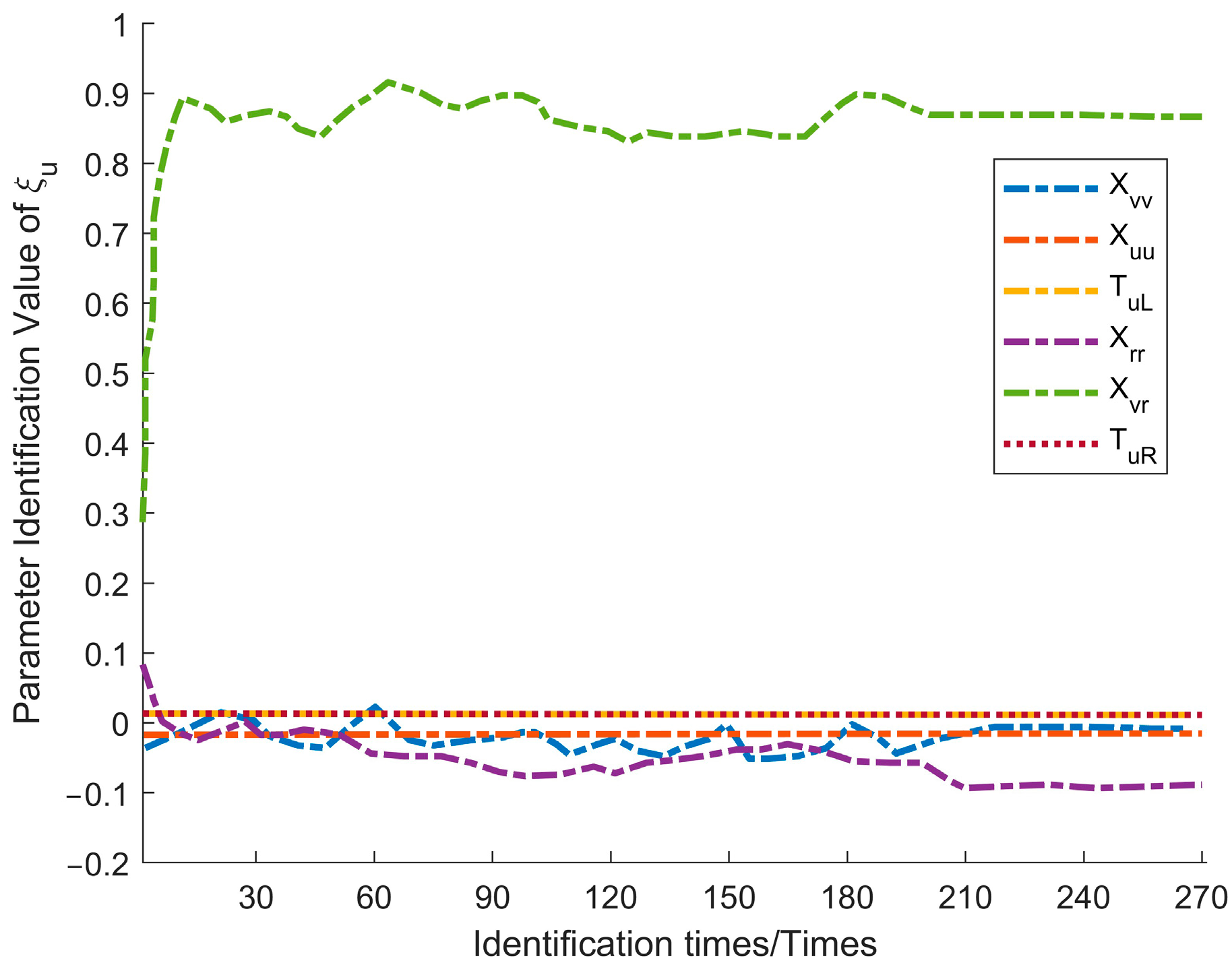
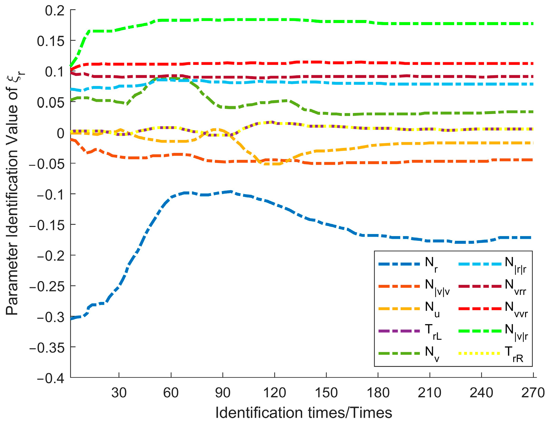
The parameter identification process for the twin USV model in this experiment is illustrated in Figure 9, Figure 10 and Figure 11. Specifically, Figure 9 presents the identification process for longitudinal dynamics parameters, Figure 10 depicts the identification of lateral dynamics parameters, and Figure 11 showcases the identification of yaw dynamics parameters.

During the parameter identification process, the dynamic sliding window-Unscented Kalman Filter (DSW-UKF) algorithm demonstrated both rapid convergence and stable performance. In the identification of longitudinal dynamics parameters, all parameters reached a stable convergence attitude after approximately 90 iterations. Parameters $X_{vv}$, $X_{rr}$, and $X_{vr}$ exhibited minor fluctuations in the early stages but quickly stabilized, while $X_{vr}$ demonstrated a particularly strong convergence effect. Meanwhile, propulsion-related parameters ($T_{uL}$ and $T_{uR}$) remained constant, indicating high resistance to wind and wave disturbances. Lateral dynamics parameters play a crucial role in the USV’s lateral motion, which is significantly affected by environmental disturbances such as wind and waves. As a result, $Y_{ur}$ and $Y_{\left|r\right|r}$ showed large initial variations but gradually converged after multiple iterations, reflecting the adaptability of the algorithm. For yaw dynamics parameters, the overall identification process remained stable. The nonlinear parameter $N_{\left|r\right|r}$ achieved high accuracy, while the linear parameter $N_r$ exhibited minor initial fluctuations before eventually stabilizing.

Based on the above analysis, the twin model progressively enhanced its adaptive capabilities throughout the identification process. Despite initial fluctuations, the parameters ultimately converged, indicating the model’s strong adaptability to dynamic environmental changes.

After 210 iterations, all parameters had essentially converged, indicating that the twin model had reached a stable attitude. At this point, the parameter identification results from the 210th iteration (as shown in

Table 2. Identified parameter values at the 210th iteration for the 20° right turn maneuver test under wind and wave conditions.

Parameters	Value	Parameters	Parameters	Value	Parameters
$X_{vv}$	−0.13319095	$Y_{ur}$	0.58329755	$N_r$	−0.17702271
$X_{uu}$	−0.01933487	$Y_v$	−0.13801318	$N_{\left|v\right|v}$	−0.04692461
$T_{uL}$	0.00750947	$Y_r$	−0.10806983	$N_u$	−0.01698518
$X_{rr}$	0.02046881	$Y_{\left|v\right|v}$	−0.34930751	$T_{rL}$	0.00568659
$X_{vr}$	0.47497131	$Y_{\left|r\right|r}$	0.05575388	$N_v$	0.03176391
$T_{uR}$	0.00750947	$Y_{\left|v\right|r}$	0.17874066	$N_{\left|r\right|r}$	0.07858179
		$Y_u$	0.14275839	$N_{vrr}$	0.08986971
		$T_{vL}$	0.13710593	$N_{vvr}$	0.11225423
		$T_{vR}$	−0.07592142	$N_{\left|v\right|r}$	0.17730327
				$T_{rR}$	0.00568859

) were substituted into the twin prediction models (Equations (22) and (23)). These models, in combination with real-time fusion of actual and twin data, were then used to predict the USV’s navigation posture.

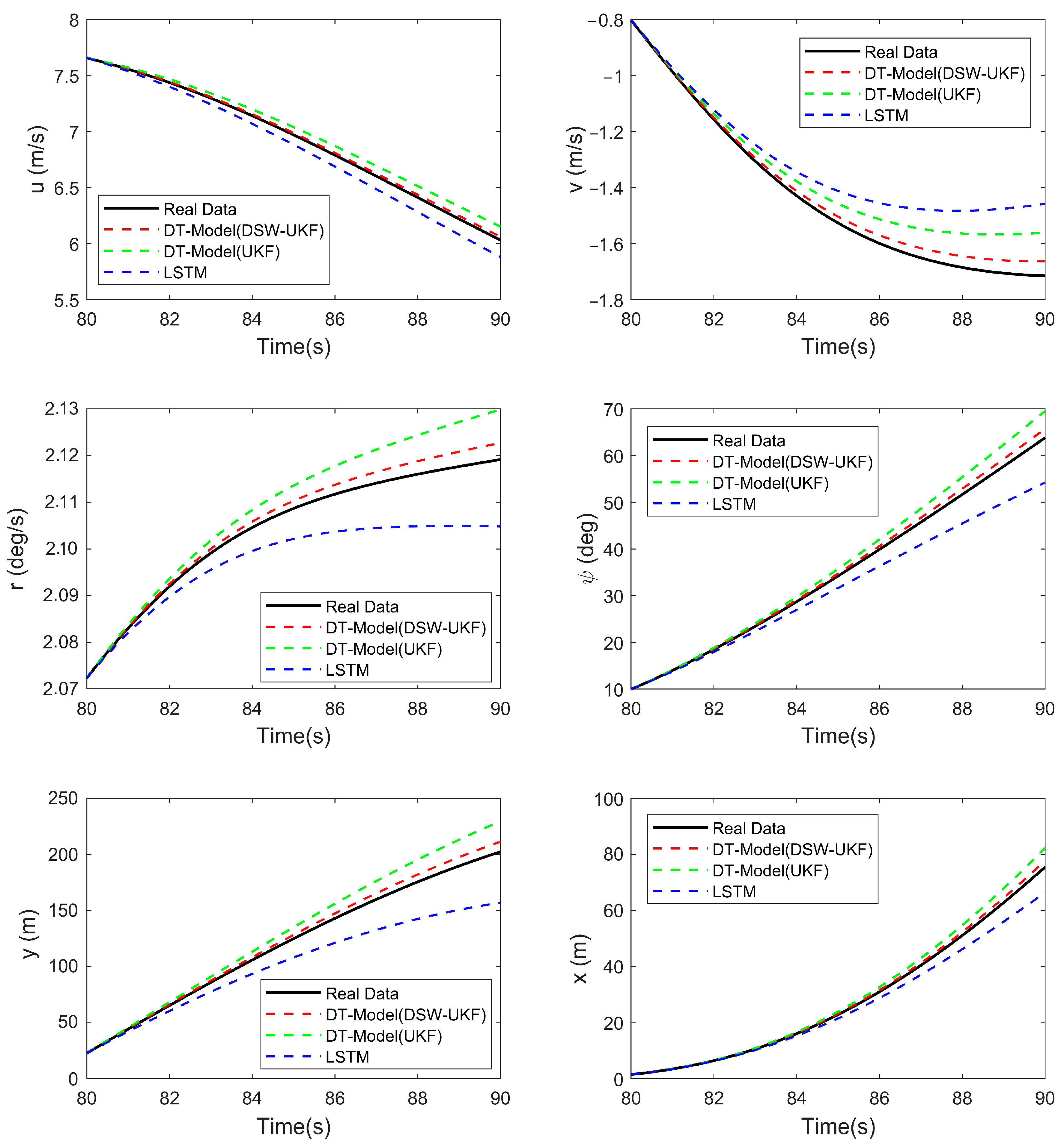
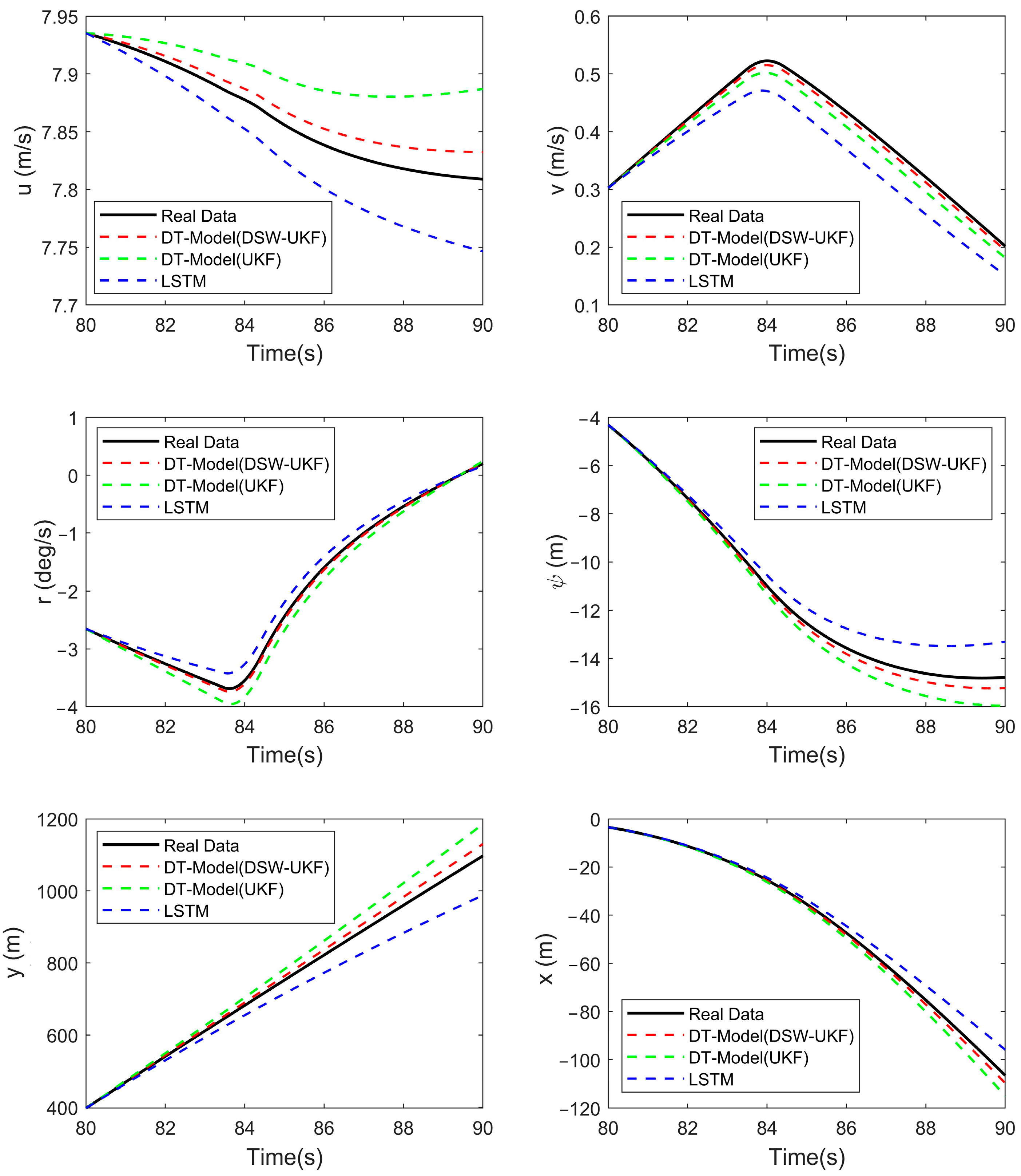
In a dynamic marine environment, factors such as wind and waves fluctuate over time, making long-term prediction accuracy difficult to guarantee. To mitigate the impact of environmental uncertainties, a 10 s prediction window was selected as a reasonable timeframe. The 10 s prediction results for the 20° right turn maneuver under wind and wave conditions are shown in Figure 12. The performance of different prediction methods varies across the results. Among them, the DT-Model (DSW-UKF)—the twin model iteratively optimized using the DSW-UKF algorithm—demonstrates the best performance across all prediction parameters. It accurately reflects the USV’s motion attitude and exhibits superior real-time adaptability and precision, particularly in handling time-varying dynamics and uncertainties.

In the attitude prediction of the 20° right turn maneuver, the proposed method demonstrates superior performance in most scenarios, accurately capturing the motion characteristics of the USV, including longitudinal and lateral velocities, yaw rate, heading angle, and positional changes. Compared with DT-Model (UKF) and the LSTM black-box model, the proposed approach achieves predictions that are consistently closer to the actual values, particularly in the eastward position and yaw rate estimation, where it exhibits higher accuracy. In contrast, the DT-Model (UKF) and LSTM black-box model show noticeable prediction deviations in certain cases. Specifically, the LSTM model exhibits larger errors in lateral velocity, heading angle, and position predictions. Overall, the DT-Model (DSW-UKF) demonstrates strong adaptability and high prediction accuracy in handling complex motion dynamics, making it a more reliable approach for USV attitude forecasting.

4.3. Scenario 2: Real-Time Attitude Prediction of a 20°/−20° Z-Type Maneuver Under Wind and Wave Conditions

The USV 20°/−20° Z-type maneuvering test was conducted under the same sea conditions. At the rated speed, the vessel first operated with a rudder angle of 20° for a certain period, followed by a period with a rudder angle of −20°, maintaining the same duration. To minimize random effects, the test was repeated four times. Data from 0 to 80 s of the test were selected for the parameter identification of the USV digital twin model.

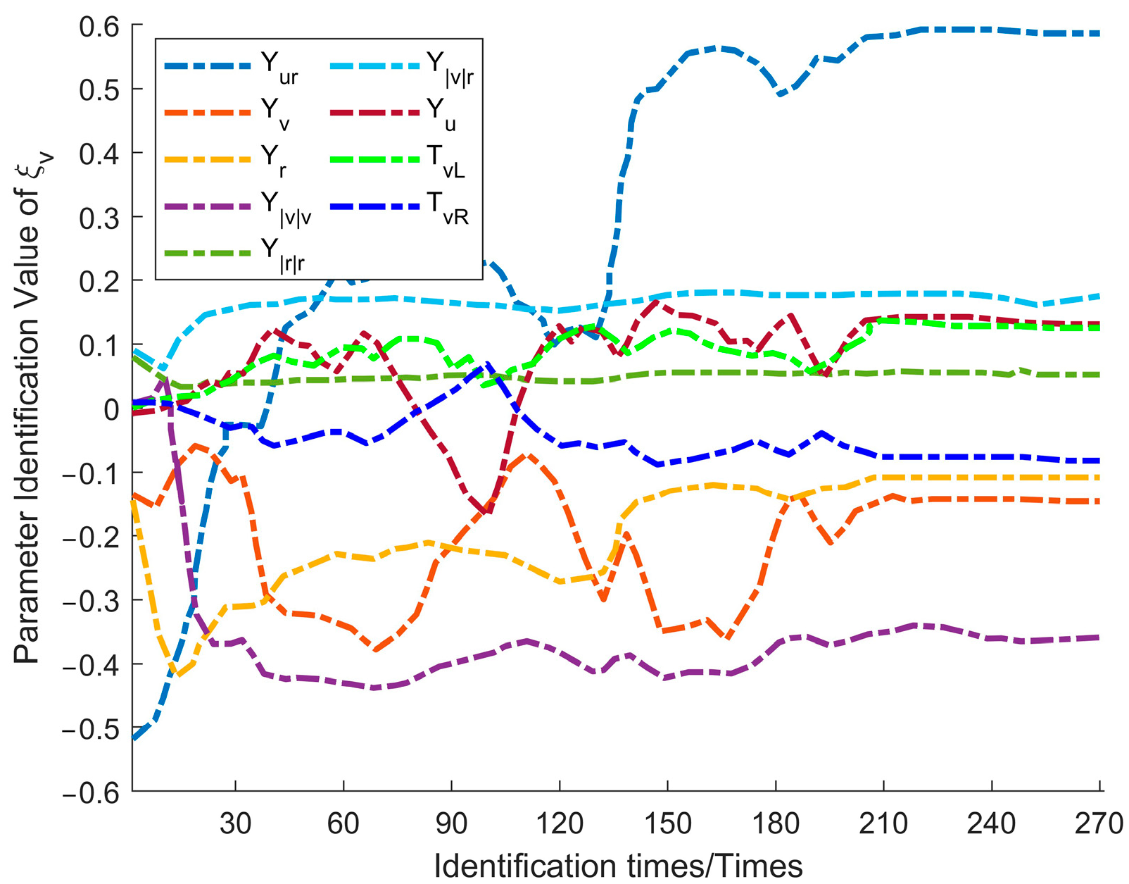
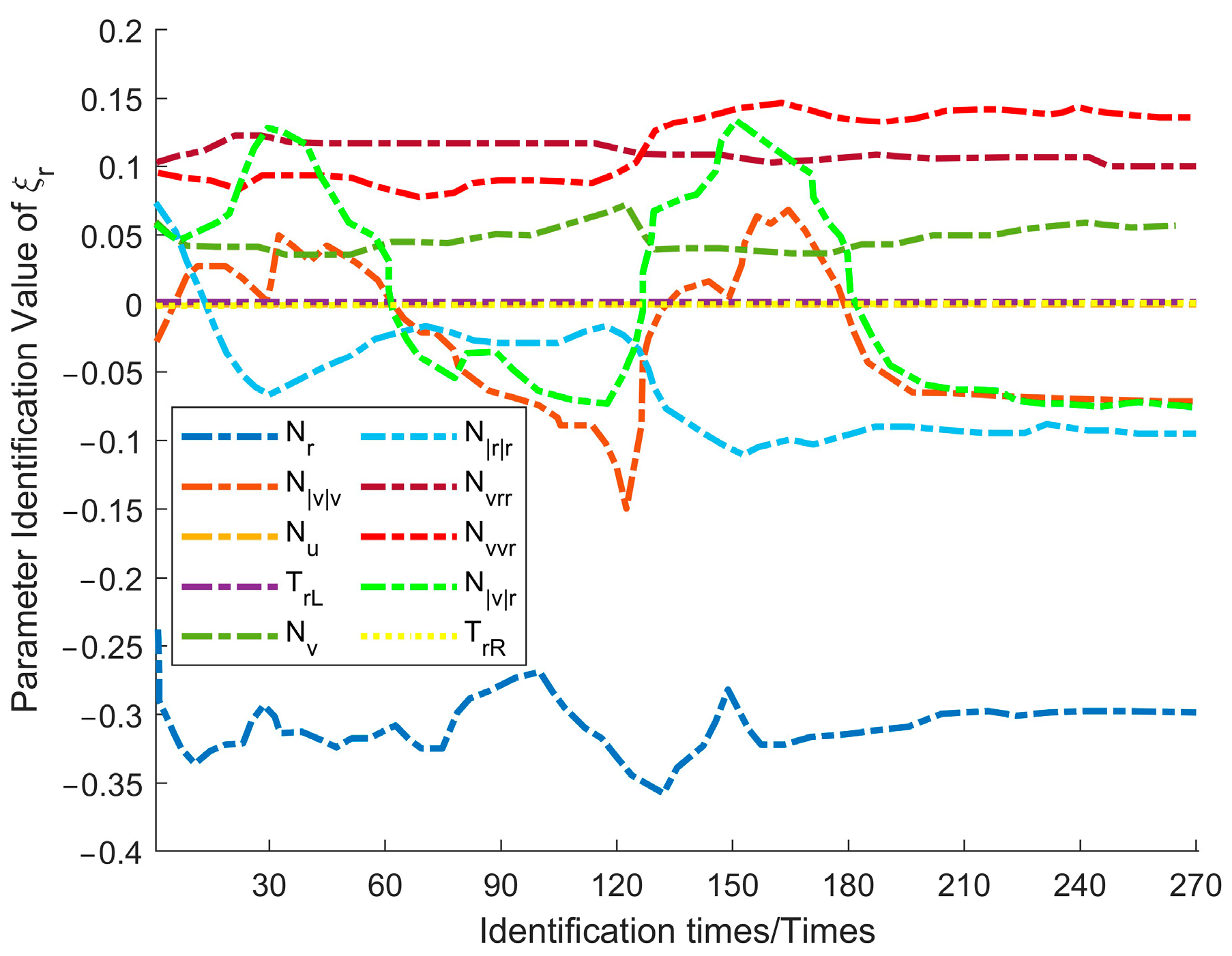
The parameter identification process for the twin USV model in this experiment is illustrated in Figure 13, Figure 14 and Figure 15. Specifically, Figure 13 presents the identification process for longitudinal dynamics parameters, Figure 14 depicts the identification of lateral dynamics parameters, and Figure 15 showcases the identification of yaw dynamics parameters.

In the 20°/−20° Z-type maneuver test under wind and wave conditions, the longitudinal dynamics parameters (e.g., $X_{vv}$ and $X_{uu}$) exhibited significant fluctuations due to frequent acceleration and deceleration as well as wave disturbances. However, they eventually converged rapidly, indicating that the model effectively captured the dynamic balance between thrust and resistance.

The lateral dynamics parameters were strongly influenced by sideslip effects and lateral wave forces, leading to continuous variations and a slower convergence rate. Similarly, yaw parameters experienced delayed convergence due to rapid turning maneuvers and nonlinear rudder effects.

Overall, the twin model dynamically adjusted in response to environmental variations throughout the identification process. This adaptability highlights the model’s strong capability to handle complex motion dynamics under challenging marine conditions.

Compared to the right turn maneuver test, the Z-type maneuver imposes higher demands on lateral and yaw responses. However, the algorithm continues to demonstrate strong robustness and high accuracy in handling these challenges. The results from both experiments indicate that the proposed algorithm is well suited for various maneuvering scenarios.

As in the previous test, the parameter identification results from the 210th iteration (detailed in

Table 3. Identified parameter values at the 210th iteration for the 20°/−20° Z-type maneuver test under wind and wave conditions.

Parameters	Value	Parameters	Parameters	Value	Parameters
$X_{vv}$	0.87067625	$Y_{ur}$	0.32354393	$N_r$	−0.29850031
$X_{uu}$	−0.01520207	$Y_v$	−0.07585661	$N_{\left|v\right|v}$	−0.06855151
$T_{uL}$	0.01141719	$Y_r$	−0.53618141	$N_u$	−0.00045943
$X_{rr}$	−0.09341181	$Y_{\left|v\right|v}$	−0.32916798	$T_{rL}$	0.00136872
$X_{vr}$	0.85951994	$Y_{\left|r\right|r}$	0.13383581	$N_v$	0.04981479
$T_{uR}$	0.01141719	$Y_{\left|v\right|r}$	0.30233231	$N_{\left|r\right|r}$	−0.09460934
		$Y_u$	−0.01204963	$N_{vrr}$	0.10663989
		$T_{vL}$	0.01002316	$N_{vvr}$	0.14198421
		$T_{vR}$	0.00686091	$N_{\left|v\right|r}$	−0.06284036
				$T_{rR}$	0.00107281

) were substituted into the twin prediction model to forecast the USV’s navigation posture.

The 10 s prediction results for the 20°/−20° Z-type maneuver under wind and wave conditions are shown in Figure 16. During this maneuver, the DT-Model (DSW-UKF) demonstrated high prediction accuracy, effectively tracking the trends of longitudinal velocity, lateral velocity, heading angle, yaw angle, and position changes. The DT-Model (UKF) also performed relatively well, closely following the actual data in most cases, though its accuracy was slightly lower than that of the improved DSW-UKF model. Meanwhile, the LSTM model, despite capturing some general trends, exhibited noticeable deviations in accuracy and detail, particularly in later-stage predictions, where its performance declined significantly.

Overall, the DT-Model (DSW-UKF) outperforms the other two methods in terms of accuracy and response speed, providing higher-precision predictions under complex wind and wave conditions.

4.4. Performance Analysis

To evaluate the performance differences between the proposed prediction method and the other two prediction methods, this paper introduces the Mean Absolute Error (MAE) and Mean Squared Error (MSE) as evaluation metrics [43] to assess the accuracy of the predicted navigation attitudes of the unmanned boat. The smaller the values of MAE and MSE, the higher the prediction accuracy. The formulas for MAE and MSE are as follows:

$$MAE={\displaystyle \frac{1}{n}}{\sum }_{i=1}^n\left|x_i-{\widehat{x}}_i\right|,$$

(53)

$$MSE={\displaystyle \frac{1}{n}}{\sum }_{i=1}^n{\left(x_i-{\widehat{x}}_i\right)}^2,$$

(54)

where $n$ represents the total number of test samples, $\widehat{x_i}$ denotes the predicted value for the i-th test sample, and $x_i$ represents the actual value for the i-th test sample.

Based on Equations (53) and (54), the MAE and Root Mean Squared Error (RMSE) for the future navigation attitudes of the unmanned boat predicted by the three methods are calculated, as shown in

Table 4. Performance analysis of USV attitude prediction method.

Scenario	Method	MAE	MSE
1	DT-Model (DSW-UKF)	0.1592	0.2292
	DT-Model (UKF)	0.1721	0.2331
	LSTM	0.1944	0.2542
2	DT-Model (DSW-UKF)	0.1733	0.1837
	DT-Model (UKF)	0.1855	0.1894
	LSTM	0.2792	0.2952

.

According to the analysis results in Table 4, in the “Wind and Wave Environment 20° Right Turn” prediction, the DT-Model (DSW-UKF) showed the best performance, with the lowest MAE (0.1592) and MSE (0.2292). In the “Wind and Wave Environment 20°/−20° Z-type Maneuver Test”, the MSE of DT-Model (DSW-UKF) decreased to 0.1837. Although the MAE slightly increased to 0.1733, it still outperformed both DT-Model (UKF) and LSTM, indicating that the model can effectively restore the navigation states of the two types of motion in the wind and wave environment through dynamic parameter calibration and noise optimization.

It is worth noting that the wind and wave environment inherently involves sensor data loss and noise, and these factors behave differently in the various experiments, further increasing the complexity of the prediction task. In a real maritime environment, the sensor data loss and noise conditions for the two motions are not identical. In this context, DT-Model (DSW-UKF) provides the most accurate predictions for both motions, demonstrating the model’s strong adaptability and robustness in complex dynamic environments. On the other hand, LSTM exhibited the largest error in all scenarios with an MAE of 0.2792, showing poor prediction performance for both motions in the wind and wave environment.

The LSTM black-box model primarily relies on training data and simulation results for motion prediction and can handle prediction tasks in various scenarios. However, in dynamic and complex environments, such as the one in Figure 16, where the USV quickly changes direction at 84 s, the predicted result for r shows large errors. In contrast, the digital twin model balances accuracy and robustness by integrating real-time sensor data and a physical model. The DSW-UKF method, through recursive updates and dynamic sliding window mechanisms, can track uncertain parameters in real-time and efficiently respond to sudden disturbances through adaptive noise estimation and feedback mechanisms. However, due to the lack of dynamic sliding window support, its ability to handle rapid changes and large amounts of data are limited, and its prediction accuracy requires improvement. The DT-Model (DSW-UKF) dynamically adjusts parameters based on recent data, adapts to time-varying characteristics, and effectively captures the motion states of the USV, providing the best prediction performance, particularly in complex dynamic environments where it shows higher stability and accuracy.

5. Conclusions

This study proposed a digital twin-driven hybrid modeling approach to address the navigation attitude prediction problem for unmanned surface vehicles (USVs). By integrating mechanistic modeling and data-driven techniques, the proposed method achieves high-precision predictions of USV navigation attitudes in complex environments. The core framework, DT-Model (DSW-UKF), is a synergistic system combining a digital twin model with an improved UKF algorithm enhanced by a dynamic sliding window mechanism.

Experimental results demonstrate that the proposed method significantly outperforms traditional approaches in terms of prediction accuracy and dynamic adaptability. The key conclusions are as follows:

• A multi-level digital twin model for USVs was developed, integrating kinematics, dynamics, control, environmental disturbance, and 3D geometric models to form a high-fidelity virtual mapping system. By aligning multi-source sensor data (e.g., GPS, IMU) with historical navigation records in both spatial and temporal dimensions, a hybrid-driven framework was established for offline training and online updates, significantly enhancing the model’s capability to represent complex dynamic behaviors.
• A dynamic sliding window-based Unscented Kalman Filter (DSW-UKF) algorithm was proposed. By adaptively adjusting the data weight window, it enables real-time estimation of hydrodynamic parameters. The algorithm dynamically corrects the digital twin model by incorporating feedback on discrepancies between the mechanistic model predictions and the actual USV motion, improving long-term prediction accuracy.
• Experimental validation under wind and wave disturbances confirms that the DT-Model (DSW-UKF) achieves more precise 10 s predictions than traditional methods, demonstrating superior adaptability to complex dynamic environments.

This study investigated the motion modeling and prediction of USV in the horizontal plane based on a 3-DOF framework. Future work will extend to a 6-DOF model to more accurately represent USV dynamics under complex sea conditions, particularly in the presence of disturbances such as wind, waves, and currents. The 6-DOF model will enhance the system’s capabilities in dynamic state estimation and control. To improve the model’s adaptability, advanced machine learning techniques, such as reinforcement learning, graph neural networks, and Transformer architectures, will be incorporated to replace or complement traditional LSTM-based approaches. These methods can capture complex motion patterns from historical data and adapt to environmental changes, improving decision-making and control efficiency. Additionally, the use of high-precision RTK technology will enhance positioning accuracy, further improving motion prediction and control. By combining 6-DOF modeling with intelligent algorithms and RTK-based precise positioning, the system is expected to improve autonomous perception and obstacle avoidance in complex environments, enhancing USV performance in applications such as coastal patrol, marine monitoring, and search and rescue.