Inter-Element Phase Error Compensated Calibration Method for USBL Arrays

Abstract

This study addresses the critical limitation of existing Ultra-Short Baseline (USBL) calibration algorithms in handling transducer positional errors and inter-element phase errors. We propose a novel positioning-calibration model based on vector projection theorem. The model achieves two key innovations: it eliminates the influence of inter-element positional errors through its structural design, and, for the first time, incorporates inter-element phase errors from acoustic array measurements as observational parameters to establish joint estimation equations for system installation angle errors and inter-element phase errors. The estimation process is implemented using an unscented Kalman filter (UKF). Simulation results demonstrate that the UKF outperforms the Gauss–Newton method (GNM), achieving estimation errors for installation angles and phase errors within 0.05°. Comparative evaluations confirm the model’s superiority over conventional calibration methods in accurately estimating installation angles under transducer positional errors. Field experiments further validate the algorithm’s effectiveness in real-world marine environments, successfully estimating system installation angle errors and inter-element phase errors to enhance final target positioning accuracy. This approach provides a practical solution to persistent calibration challenges in USBL systems.

1. Introduction

The Ultra-Short Baseline (USBL) system is an acoustic-based positioning technology characterized by its compact array dimensions, operational simplicity, and ease of installation/maintenance, making it particularly suitable for surface vessel-to-underwater target localization. The integration of USBL with Strapdown Inertial Navigation Systems (SINS) enables sustained high-precision underwater positioning for submersibles or ships, establishing SINS/USBL integrated navigation as an increasingly prominent research domain [1,2,3,4]. Critical factors affecting system accuracy include measurement errors induced by marine environmental parameters, transducer positional errors in acoustic arrays, and angular misalignment between USBL and SINS installations [5].

System calibration constitutes an essential process for enhancing the ultimate positioning accuracy of USBL systems. Imperfect coupling between USBL and SINS inevitably introduces installation errors, where a 1° heading misalignment [6] can result in horizontal positioning errors exceeding 1% of the slant range. Tang [7] proposed a two-stage parameter estimation framework, first estimating transponder positions via range intersection and then deriving error parameters using predefined criteria. Zhang [8] improved target positioning accuracy by synthesizing observational errors. Zheng [9] applied least-squares optimization for installation errors estimation, though with limited precision. Chen [10] developed an iterative calibration method analyzing individual attitude impacts on USBL performance, achieving higher accuracy but requiring circular calibration trajectories. Tong [11] proposed a dual-transponder calibration scheme capable of effectively estimating installation angle errors. However, this method requires precise knowledge of the depth difference between the two transponders, which is challenging to achieve in practical applications. Guo [12] introduced an inverted USBL calibration algorithm, where the USBL system is placed on the seabed for installation angle calibration. However, this approach is not suitable for real-world engineering applications. These methods universally rely on least-squares techniques, which exhibit noise sensitivity and permit only post-calibration batch processing rather than real-time implementation.

Recent advances address these limitations through state estimation-based approaches. Zhang [13,14] employed the unscented Kalman filter (UKF) for online installation angle calibration, demonstrating operational feasibility. Zhu [15] extended this framework to concurrently estimate SINS/USBL positional and angular errors. Wang [16] proposed a smoothed variable-structure UKF algorithm to enhance convergence stability and estimation accuracy. Zhu [17] improved precision via vector observation modeling, while Zhang [18] achieved effective errors estimation through differential calibration of sound speed and installation angle errors.

However, the aforementioned calibration algorithms focus solely on correcting the installation angle errors between the USBL and SINS systems. In addition to these errors, the positioning accuracy of the USBL system is also affected by phase errors and position errors among array elements, which result from manufacturing imperfections. These errors have not been accounted for in the existing algorithms. Moreover, since the calibration models use the target position as the observation variable, they are constrained by the positioning algorithm itself, and are therefore unable to solve for these errors within the calibration framework.

To address these challenges, this study develops a positioning algorithm employing the vector projection method and constructs a novel calibration model. Unlike conventional calibration approaches that utilize target positions as observables, our methodology establishes observation equations using phase differences between transducer elements, enabling simultaneous calibration of inter-element phase errors and installation angular errors. The algorithm’s compatibility with arbitrary array configurations allows the incorporation of physically measured transducer positions into the positioning model. Simulation and experimental results confirm the method’s effectiveness in estimating both installation angle errors and phase discrepancies between elements, demonstrating practical applicability in real underwater environments.

2. Principle of SINS/USBL Combination Positioning

The integrated positioning system enables high-precision underwater target localization by combining a SINS with a USBL acoustic positioning system. The system operates through two principal technical components. The USBL subsystem employs an underwater transponder deployed at the target location and a ship-mounted acoustic transducer array. Through precise measurement of acoustic signal propagation time between the transducer array and transponder, it establishes the target’s relative spatial coordinates relative to the host vessel.

The coordinate transformation mechanism then processes these relative measurements using SINS-provided real-time navigation data, including vessel attitude parameters (roll, pitch, and heading angles) and positional information. By implementing lever arm compensation and coordinate system conversion algorithms, the system translates the USBL-derived relative coordinates into an Earth-fixed geographic reference frame. This technical integration effectively mitigates positioning errors caused by vessel dynamics and environmental interference, resulting in enhanced operational accuracy that reaches centimeter-level precision under optimal conditions.

The combined navigation solution demonstrates superior performance in complex underwater environments where traditional positioning methods face limitations, achieving reliable target tracking through advanced multi-sensor fusion techniques.

2.1. Principle of USBL Acoustic Positioning

Figure 1 illustrates the transducer array configuration of the USBL system, which adopts a uniform five-element circular planar geometry.

The vector projection method is a direction-finding algorithm for two-element arrays operating under far-field plane-wave conditions. Figure 2 demonstrates a typical two-element direction finding system, where the key parameter is the incident angle θ between the signal propagation direction and the array baseline, with θ ranging from 0° to 180°. The fundamental relationship between this angular parameter and the phase differences observed between transducer elements is mathematically expressed in Equation (1). This formulation establishes the theoretical foundation for converting phase measurements into spatial orientation information, enabling precise directional estimation through systematic analysis of acoustic signal characteristics.

$$\cos (\mathsf{\theta })={\displaystyle \frac{c{\phi }_{mn}}{2\pi f{d}_{mn}}}$$

(1)

where c is the sound speed, ${\phi }_{mn}$ is the phase errors between the element m and element n, f is the signal frequency, and $d_{mn}$ is the distance between the elements.

Set $X_m=(x_m,y_m,z_m)$ and $X_n=(x_n,y_n,z_n)$, so that the positioning coordinate of the target is $X_o=(x_s,y_s,z_s)$.

According to the vector projection theorem, Equation (2) is:

$$\cos (\mathsf{\theta })={\displaystyle \frac{X_o\cdot X_{nm}}{d_{mn}{R}_s}}$$

(2)

where $X_o$ and $X_{mn}$ represent the direction vectors of the target and the baseline mn, respectively, defined as $X_o=(x_s,y_s,z_s)$ and $X_{mn}=(x_m-x_n,y_m-y_n,z_m-z_n)$. The notation $(\cdot )$ denotes the vector dot product, and $R_s$ indicates the distance from the target to the transducer array.

Since the angle calculated by vector projection is identical to that obtained through two-element direction finding, Equations (1) and (2) can be combined to derive Equation (3).

$$x_s(x_n-x_m)+y_s(y_n-y_m)+z_s(z_n-z_m)={\displaystyle \frac{R_{s}c{\phi }_{mn}}{2\pi f}}$$

(3)

In this Equation, the coordinates of transducer elements can be predetermined through laser ranging measurements of the array configuration, thus serving as known parameters. Target coordinate determination requires establishing three equations, corresponding to three baselines. However, given the planar array geometry, Equation (4) introduces a geometric constraint that enables the reformulation of Equation (3) into Equation (5).

$$z_m=z_n$$

(4)

$$x_s(x_m-x_n)+y_s(y_m-y_n)={\displaystyle \frac{R_{s}c{\phi }_{mn}}{2\pi f}}$$

(5)

By selecting two additional transducer elements, p and q, with coordinates $X_p=(x_p,y_p,z_p)$ and $X_q=(x_q,y_q,z_q)$, we ultimately derive Equation (6). The target’s depth is then calculated using the Pythagorean theorem, as formulated in Equation (7).

$$\left[\begin{array}{l}{x}_s\\ y_s\end{array}\right]={\displaystyle \frac{R_{s}c}{2\pi f}}{\left[\begin{array}{cc}{x}_m-x_n& y_m-y_n\\ x_p-x_q& y_p-y_q\end{array}\right]}^{-1}\left[\begin{array}{l}{\phi }_{mn}\\ {\phi }_{pq}\end{array}\right]$$

(6)

$$z_s=-\sqrt{{R_s}^2-{x_s}^2-{y_s}^2}$$

(7)

In summary, this localization algorithm imposes no specific constraints on transducer placement geometry, requiring only prior positional measurements of all array elements to enable reliable acoustic target localization.

2.2. Principle of Coordinate System Transformation

In this study, the transformation between three coordinate systems is considered: the acoustic coordinate system, the vessel-mounted coordinate system, and the geodetic coordinate system. As shown in Figure 3, assuming that the coordinate systems of the SINS and USBL are aligned, the acoustic coordinate system is represented as the A-frame, where the origin O_A is located at the center of the array. The X_A-axis is aligned with the direction of the first array element, the Y_A-axis is oriented vertically upward from the array plane, and the X_A-axis, Y_A-axis and Z_A-axis form a left-handed coordinate system. The vessel-mounted coordinate system is denoted as the S-frame, with its origin coinciding with that of the acoustic coordinate system. In this system, the X_S-axis points eastward, the Y_S-axis points northward, and the Z_S-axis is directed vertically upward from the X_SO_sY_S plane. The geodetic coordinate system is represented as the G-frame, with its origin located at the center of the DGPS antenna. In this system, the X_G-axis points eastward, the Y_G-axis points northward, and the Z_G-axis is oriented vertically upward from the X_GO_GY_G plane.

Based on the definitions of these coordinate systems, the transformation of an underwater target’s position into the geodetic coordinate system requires first rotating the acoustic coordinate system into the vessel-mounted coordinate system, followed by a translation into the geodetic coordinate system.

In this study, the Cardan rotation principle [19] is employed for coordinate system rotations, following the Z-Y-X rotation sequence. The rotation angles are provided by the atitude sensors. Let $\kappa$ denote the yaw angle corresponding to rotation about the Z-axis, $\omega$ the pitch angle corresponding to rotation about the Y-axis, and $\rho$ the roll angle corresponding to rotation about the X-axis. All three angles follow the right-hand rule, where a positive rotation is defined such that when the right-hand thumb points along the axis of rotation, the curled fingers indicate the direction of positive rotation.

The relations of the three rotation matrices are as follows:

$$R_{\mathrm{Z}}(\kappa )=\left(\begin{array}{ccc}\cos \kappa & \sin \kappa & 0\\ -\sin \kappa & \cos \kappa & 0\\ 0& 0& 1\end{array}\right)$$

(8)

$$R_{\mathrm{Y}}(\omega )=\left(\begin{array}{ccc}\cos \omega & 0& \sin \omega \\ 0& 1& 0\\ -\sin \omega & 0& \cos \omega \end{array}\right)$$

(9)

$$R_{\mathrm{X}}(\rho )=\left(\begin{array}{ccc}1& 0& 0\\ 0& \cos \rho & \sin \rho \\ 0& -\sin \rho & \cos \rho \end{array}\right)$$

(10)

Let $R_A^S$ represent the rotation matrix from the A-frame to the S-frame, and the expression for $R_A^S$ is

$$R_A^S=R_{\mathrm{Z}}(\kappa )R_{\mathrm{Y}}(\omega )R_{\mathrm{X}}(\rho )$$

(11)

In practical operations, the vessel’s position continuously changes, causing the origins of the three coordinate systems to shift accordingly. To facilitate observation, a fixed reference point is typically chosen, such as the dock or the vessel’s position at a specific moment. The target position is then expressed relative to this fixed point. Consequently, the final formula for the target coordinates is given by:

$$P=R_A^S{P}_A+P_G-P_l+P_{GA}$$

(12)

where $P_A$ represents the target coordinates in the acoustic coordinate system, $P_G$ denotes the coordinates of the antenna center, $P_l$ represents the coordinates of the fixed reference point, and $P_{GA}$ corresponds to the coordinates of the acoustic array center relative to the antenna center. In summary, the block diagram of the combined positioning process is as shown in Figure 4.

3. Principle of System Calibration

In practical applications, system installation errors and manufacturing imperfections can degrade the accuracy of target positioning. However, due to the nature of the positioning algorithm, the array element positions can be measured in advance, allowing the installation errors of the array elements to be neglected. This paper focuses on analyzing the installation angle errors of the SINS and the USBL system, as well as the phase inconsistencies among USBL array elements. During the calibration process, a transponder is usually fixed; that is, the coordinate position of the transponder is known. Since the coordinate position of the vessel can be provided by GPS, the relative coordinates between the vessel and the transponder in the calibration model can be regarded as known quantities.

The installation angle errors between SINS and USBL refer to the misalignment between their respective coordinate frames during operation. Let the installation errors angles be represented as $\varphi =[\alpha ,\beta ,\gamma ]$, where $\alpha$ denotes the rotational errors around the Z-axis, $\beta$ around the Y-axis, and $\gamma$ around the X-axis. The installation errors matrix is derived using Equation (11), where $R_O^A$ represents the rotation matrix that transforms the initial USBL-based target position into the acoustically determined target position. Additionally, phase inconsistencies among array elements arise due to manufacturing imperfections, as the fabrication process cannot ensure complete uniformity. Let $\delta$ represent the errors magnitude, as described in Equation (13)

$$\delta =[\alpha ,\beta ,\gamma ,{{\phi }^{\prime }}_{12},{{\phi }^{\prime }}_{23},{{\phi }^{\prime }}_{34},{{\phi }^{\prime }}_{45},{{\phi }^{\prime }}_{51}]$$

(13)

where ${{\phi }_{12}}^{\prime }$, ${{\phi }_{23}}^{\prime }$, ${{\phi }_{34}}^{\prime }$, ${{\phi }_{45}}^{\prime }$, ${{\phi }_{51}}^{\prime }$ represent the phase processing errors between the elements, respectively.

The estimation of errors parameter $\delta$ a requires the establishment of observation equations based on measured phase differences between transducer elements. Specific steps are as follows:

Step 1. According to Equation (5), the observed phase difference between m and n can be expressed as

$${\phi }_{mn}={\displaystyle \frac{2\pi f}{R_{s}c}}\left[\begin{array}{l}{x}_s\\ y_s\\ z_s\end{array}\right]\left[\begin{array}{ccc}{x}_m-x_n& y_m-y_n& z_m-z_n\end{array}\right]+{{\phi }^{\prime }}_{mn}$$

(14)

Step 2. During calibration procedures, a transponder is typically fixed at a known coordinate $P_l$. The final target position $P$, the antenna center coordinate $P_G$, and the acoustic array center coordinate $P_{GA}$ relative to the antenna center are all treated as known quantities. The expression for $P_S$ is formulated as:

$$P_S=P+P_l-P_G-P_{GA}$$

(15)

According to the installation errors rotation matrix can be obtained as follows:

$$P_S=R_A^S{R}_O^A{X}_o$$

(16)

Step 3. Bringing Equation (16) into Equation (14) gives Equation (17).

$${\phi }_{mn}={\displaystyle \frac{2\pi f}{R_{s}c}}{(R_O^A)}^{-1}{(R_A^S)}^{-1}\left[\begin{array}{l}x\\ y\\ z\end{array}\right]\left[\begin{array}{ccc}{x}_m-x_n& y_m-y_n& z_m-z_n\end{array}\right]+{{\phi }^{\prime }}_{mn}$$

(17)

At this stage, the coordinate $\left[\begin{array}{ccc}x& y& z\end{array}\right]$ represents the relative position between the target and the acoustic baseline array in the geodetic coordinate system. Given that there are a total of five phase difference errors, five observation equations can be established accordingly. Based on Equation (17), the observation equations are formulated as shown in Equation (18).

$$z_k={[{\phi }_{12}{\phi }_{23}{\phi }_{34}{\phi }_{45}{\phi }_{51}]}^{\mathrm{T}}=h(\alpha ,\beta ,\gamma ,{{\phi }^{\prime }}_{12},{{\phi }^{\prime }}_{23},{{\phi }^{\prime }}_{34},{{\phi }^{\prime }}_{45},{{\phi }^{\prime }}_{51})+v$$

(18)

where $v$ represent the observation noise.

The observation equation exhibits inherent nonlinearity. A conventional approach for handling nonlinear problems is the Gauss–Newton method (GNM), which linearizes the system through Taylor series expansion, enabling parameter updates via linear least-squares solutions at each iteration. However, the Jacobian matrix derived from Equation (18) demonstrates significant complexity. The iterative nature of GNM requires repeated linear approximations using local Taylor expansions around current parameter estimates, followed by linear least-squares optimization until convergence or maximum iterations are reached—a process incurring substantial computational overhead. To improve both estimation accuracy and computational efficiency, this study employs the UKF for installation errors estimation, eliminating the need for explicit Jacobian calculations while maintaining recursive estimation capabilities.

Principle of UKF

The UKF is a Kalman filtering algorithm designed for nonlinear estimation problems. Its core principle involves strategically selected sampling points (sigma points) that capture the statistical characteristics of state distributions. Through the unscented transform (UT), these sigma points address nonlinearities in the observation Equation (17) by propagating through system dynamics. Unlike the GNM requiring explicit iterative optimization, the UKF updates state estimates recursively at each timestep using incoming measurement data. This operational mechanism enables real-time parameter estimation through continuous adaptation to new observations without iterative computations. The sigma points’ nonlinear transformation provides more accurate mean and covariance estimates than conventional linearization approaches, yielding superior estimation precision. These attributes make the UKF particularly suitable for practical engineering applications requiring dynamic state tracking [20,21].

Given the constant nature of installation errors, the state vector remains time-invariant with $x_k=f(x_k)$. To facilitate subsequent algorithmic analysis, we integrate Equations (13) and (18) to formulate the system’s state-space model as follows:

$$\left\{\begin{array}{l}{x}_k=f(x_{k-1})+u_{k-1}\hfill \\ z_k=h(x_k)+v_k\hfill \end{array}\right.$$

(19)

The UKF implementation involves the following three sequential stages: initialization, prediction, and update.

• Initialization

The initialization phase establishes the state vector’s initial mean values and covariance matrix while generating sigma points through the procedure defined in Equation (20). These sigma points are systematically distributed around the initial state estimate, with their quantity determined by the state dimension n as 2n + 1, as mathematically specified in Equation (21).

$$\left\{\begin{array}{l}{\widehat{x}}_0=E[x_0]\\ P_0=E[(x_0-{\widehat{x}}_0){(x_0-{\widehat{x}}_0)}^T]\end{array}\right.$$

(20)

$$\left\{\begin{array}{l}\begin{array}{cc}{\chi }_0={\widehat{x}}_k,& i=0\end{array}\\ \begin{array}{cc}{\chi }_i={\widehat{x}}_k+{(\sqrt{(n+\lambda )P_k})}_i,& i=1,\dots ,n\end{array}\\ \begin{array}{cc}{\chi }_i={\widehat{x}}_k-{(\sqrt{(n+\lambda )P_k})}_i,& i=n+1,\dots ,2n\end{array}\end{array}\right.$$

(21)

where $\lambda$ represents the distribution weight of sigma points; its expression is

$$\lambda =a^2\left(n+u\right)-n$$

(22)

where a determines the distribution of Sigma points around the state variable, the influence of higher-order terms on the system of a nonlinear system can be reduced by adjusting the size of a, which is usually 0.001, and u is a scale factor, usually 0.

The prediction stage propagates these sigma points through the system dynamics model to forecast state evolution, while the update stage incorporates new measurement data to refine the estimates. This structured approach eliminates the need for Jacobian matrix calculations required in conventional nonlinear filtering methods.

2.

Prediction

To obtain the mean and variance of the predicted state, each sigma sampling point needs to be predicted first, and the formula is shown in Equation (23).

$${\chi }_{i,k|k-1}=f({\chi }_{i,k-1})$$

(23)

The expression of prediction state mean and prediction covariance is

$$\left\{\begin{array}{l}{\widehat{x}}_{k|k-1}={\displaystyle {\sum }_{i=0}^{2n}{W}_m^i{\chi }_{i,k|k-1}}\\ P_{k|k-1}={\displaystyle {\sum }_{i=0}^{2n}{W}_c^i({\chi }_{i,k|k-1}-{\widehat{x}}_{k|k-1}){({\chi }_{i,k|k-1}-{\widehat{x}}_{k|k-1})}^T+Q_{k-1}}\end{array}\right.$$

(24)

where $Q_{k-1}$ represents the covariance matrix of process noise, and $W_m^i$ and $W_c^i$, respectively, represent the weight of mean and covariance calculation, whose expressions are shown in Equation (25).

$$\left\{\begin{array}{l}{W}_m^0={\displaystyle \frac{\lambda }{n+\lambda }}\\ W_c^0={\displaystyle \frac{\lambda }{n+\lambda }}+(1-a^2+b)\\ W_m^i=W_c^i={\displaystyle \frac{\lambda }{2(n+\lambda )}},i=1,\dots ,2n\end{array}\right.$$

(25)

where b is used to introduce the weight of the prior distribution, which, for Gaussian distributions, usually takes a value of 2.

3.

Update

In the update stage, the observation model should be applied to each sigma point first, as shown in Equation (26)

$$Z_{i,t|t-1}=h({\chi }_{i,t|t-1})$$

(26)

The calculated predicted observed mean and observed covariance are shown in Equation (27).

$$\left\{\begin{array}{l}{\widehat{z}}_{k|k-1}={\displaystyle {\sum }_{i=0}^{2n}{W}_m^i{Z}_{i,t|t-1}}\\ P_{k|k-1}^{zz}={\displaystyle {\sum }_{i=0}^{2n}{W}_c^i(Z_{i,t|t-1}-{\widehat{z}}_{k|k-1}){(Z_{i,t|t-1}-{\widehat{z}}_{k|k-1})}^T+R_{k-1}}\end{array}\right.$$

(27)

where $R_{k-1}$ represents the covariance matrix of observation noise, while the cross covariance $P_{k|k-1}^{xz}$ of state and observation can be obtained by Equation (28).

$$P_{k|k-1}^{xz}={\displaystyle {\sum }_{i=0}^{2n}{W}_c^i(Z_{i,t|t-1}-{\widehat{x}}_{k|k-1}){(Z_{i,t|t-1}-{\widehat{z}}_{k|k-1})}^T}$$

(28)

Finally, the Kalman gain can be calculated by Equations (19), (24), (27) and (28). The state estimation can be updated as shown in Equation (29).

$$\left\{\begin{array}{l}{K}_k=P_{k|k-1}^{xz}{(P_{k|k-1}^{zz})}^{-1}\\ {\widehat{x}}_k={\widehat{x}}_{k|k-1}+K_k(z_k-{\widehat{z}}_{k|k-1})\\ P_k=P_{k|k-1}-K_k{P}_{k|k-1}^{zz}{(K_k)}^T\end{array}\right.$$

(29)

The above is the whole process of UKF, and the final result, ${\widehat{x}}_k$, is the estimated errors.

The computational overhead of the two algorithms can be analyzed starting from the computational complexity. The UKF demonstrates linear computational complexity $O(N)$, where N denotes data segment length, whereas the GNM requires $O(MN)$ operations due to its iterative nature across the entire dataset, with M representing the preset iteration count. This complexity disparity, compounded by GNM’s Jacobian matrix computations that escalate processing overhead in large datasets, results in significantly longer calibration durations for GNM compared to UKF.

The process of system calibration is shown in Figure 5

4. Simulation Analysis

In order to verify the calibration algorithm proposed in this paper, a simulation test was designed. The sensors involved in the simulation are a real-time Kinematics Global Positioning System (GPS-RTK), USBL, and SINS. The sensor errors are shown in

Table 1. Main technological parameters of sensors.

Sensors	Parameters	Value
GPS-RTK	Position accuracy	0.02 m
SINS	Heading	0.01°
	Pitch	0.005°
	Roll	0.005°

. The simulation software uses Scilab, v2024.1.0. Since the simulation in this paper is mainly for verifying the calibration model, the sound velocity error is not considered in the simulation model for the time being. The solutions to the actual sound velocity error will be mentioned in the subsequent field experiment chapter.

The underwater acoustic signal uses a 25 Khz CW signal with a pulse width of 5 ms and the USBL system uses notch filters to detect and estimate the parameters of CW signal. A simulation experiment was constructed to investigate the performance of the proposed method. Specifically, 1000 Monte Carlo trials were conducted under various signal-to-noise ratio (SNR) conditions. The root mean square error (RMSE) metric was employed to compute the final phase error results, providing a quantitative assessment of the accuracy and stability of the estimation process. The relationship between the phase error detected by the USBL system and the SNR is shown in Figure 6.

During calibration procedures, the transponder is submerged at a known position. The SINS/USBL equipment, rigidly mounted underwater, incorporates high-precision RTK positioning. The survey vessel carrying the USBL system maneuvers around the transponder. At each trajectory position, the acoustic array communicates with the transponder while recording the following three data streams: RTK-derived vessel coordinates, SINS-calculated attitude parameters, and USBL-acquired hydroacoustic measurements. Figure 7 simulates this calibration geometry, with the transponder fixed at coordinates (0, 0, −200). The USBL array configuration follows the uniform five-element circular geometry shown in Figure 1, featuring a 16.25 cm array radius. Data acquisition occurs at 0.1 s intervals over a 729.1 s operational period. The SNR is set to 0 dB.

Set the installation errors angle as $[\alpha ,\beta ,\gamma ]=[10,5,-3]$ and the phase errors between each element as $[{{\phi }^{\prime }}_{12},{{\phi }^{\prime }}_{23},{{\phi }^{\prime }}_{34},{{\phi }^{\prime }}_{45},{{\phi }^{\prime }}_{51}]=[6,4,7,-8,-7]$, in units of degrees, then the errors are estimated by UKF as shown in the figure below.

As shown in Figure 8 and Figure 9, the UKF estimation results demonstrate convergence after 600 s, with all error estimates maintaining errors within 0.05° of true values. Consequently, the mean values from 600 s to 700 s are adopted as final error estimates. For performance comparison, the same data segment is processed using GNM with 400 iterations, where the last iteration output serves as GNM’s estimate.

Table 2. The results of two algorithms.

Parameters	True Value	Methods
		UKF	GNM
$\alpha$	10°	10.0037°	10.0113°
$\beta$	5°	4.9884°	5.0211°
$\gamma$	−3°	−2.9704°	−3.0271°
${{\phi }^{\prime }}_{12}$	6°	5.9926°	6.0149°
${{\phi }^{\prime }}_{23}$	4°	4.0101°	4.0303°
${{\phi }^{\prime }}_{34}$	7°	7.0083°	6.9885°
${{\phi }^{\prime }}_{45}$	−8°	−8.0096°	−8.0174°
${{\phi }^{\prime }}_{51}$	−7°	−7.0068°	−6.9822°

presents both algorithms’ estimation errors against ground truth values. For installation angle errors, UKF achieves errors of 0.0037°, −0.0116°, and 0.0296°, while GNM yields 0.0113°, 0.0211°, and −0.0271°. Regarding inter-element phase errors, UKF exhibits errors of −0.0074°, 0.0101°, 0.0083°, −0.0096°, and −0.0068°, compared to GNM’s 0.0149°, 0.0303°, −0.0115°, −0.0174°, and 0.0178°. These results quantitatively confirm UKF’s superior estimation accuracy over GNM. Figure 10 shows the influence of the errors estimated by UKF and GNM on the final positioning results. It can be seen that both algorithms can calibrate and converge the positioning results near the target position, demonstrating the effectiveness of the calibration model.

Table 3. Statistical errors before and after calibration in the simulation test.

Methods	X-Axis	Y-Axis	Z-Axis
Original	35.739 m	51.421 m	48.141 m
UFK	1.432 m	1.441 m	1.724 m
GNM	1.691 m	1.686 m	2.402 m

analyzes the positioning errors in each direction. It can be seen that the positioning results obtained by using the estimated parameters of UKF have higher accuracy.

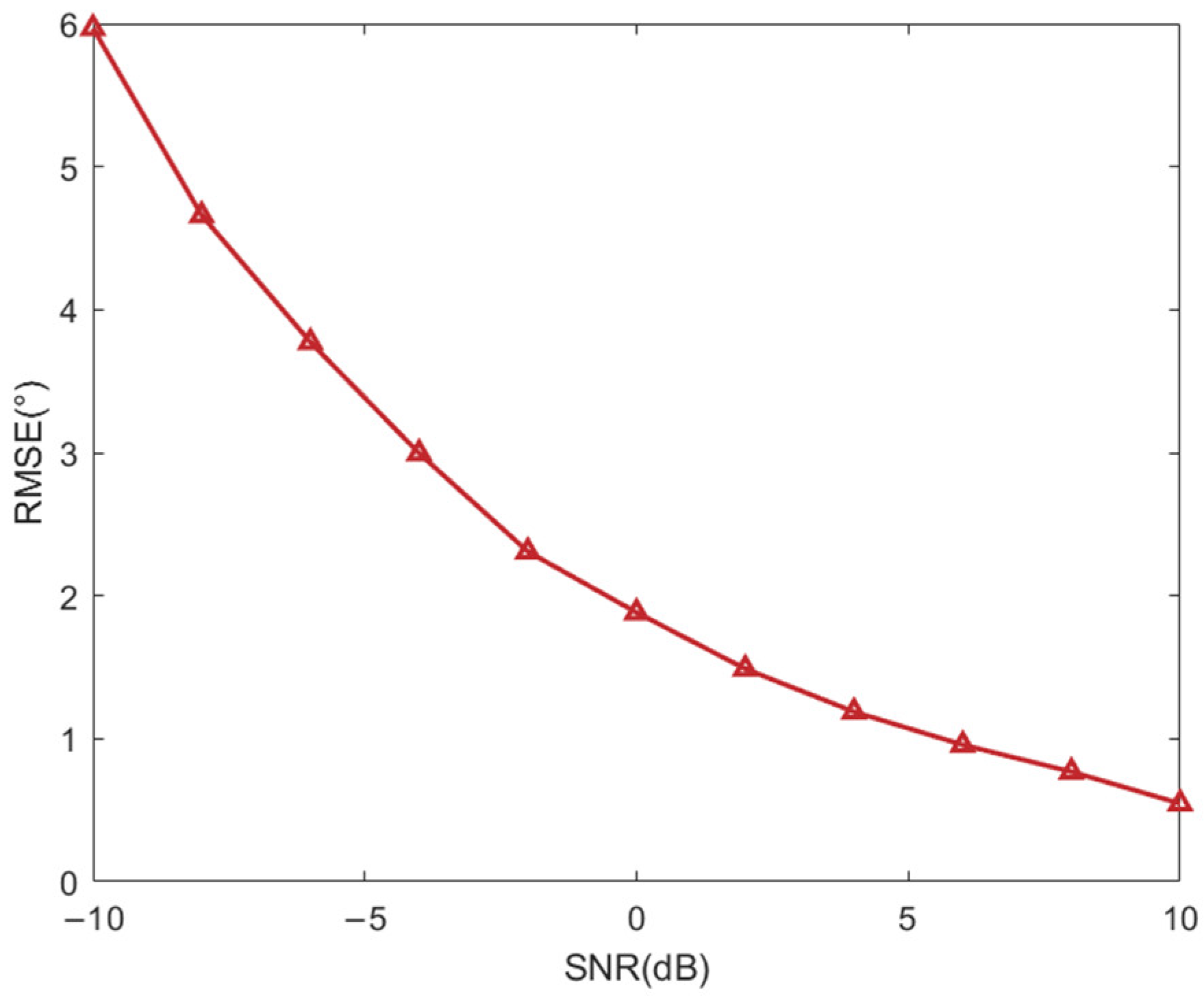
In order to verify the parameter estimation performance of UKF and GNM under different SNR, a simulation experiment was established and the SNR range was set from −10 dB to 10 dB. The vessel trajectory is shown in Figure 7. Since the simulation experiment is solely focused on investigating the influence of the SNR on the estimation accuracy, the error angles are set identically to those in the previous context. The number of Monte Carlo experiments is set to 1000, and the final error result is the RMSE. For the sake of convenience, only the relationship between the error angle $\alpha$ and the SNR is observed. The result is shown in Figure 11.

It can be seen from Figure 11 that the estimation accuracy of UKF is higher than that of GNM in all SNR cases, which indicates that UKF has higher accuracy in parameter estimation.

A comparative analysis of computational expenditure was conducted using calibration simulation datasets.

Table 4. Computing time of two algorithms.

Methods	Computing Time (s)
UKF	1.044
GNM	240.713

details the execution time comparison, revealing that UKF’s computational speed surpasses GNM by approximately 230.5 times in the tested data scenario. The UKF’s efficiency advantage stems from its non-iterative recursive framework that avoids complex matrix inversions, making it particularly advantageous for real-time marine positioning applications requiring rapid calibration updates.

To validate the calibration algorithm’s immunity to array geometry errors (applicable to arbitrary configurations), the array was reconfigured into a quadrilateral orthogonal layout with each element positioned 0.1625 m from the origin. Element 4 was intentionally displaced 0.01 m along the y-axis, as illustrated in Figure 12. Set the installation Angle errors as $[\alpha ,\beta ,\gamma ]=[2,2,2]$. With preset phase errors intentionally excluded, this configuration specifically evaluates array displacement impacts on installation angular errors estimation. Method 1 represents the conventional calibration model, while Method 2 denotes the proposed model, both employing UKF for errors estimation.

Figure 13 reveals critical limitations of Method 1: when Element 4 position deviates, the conventional model’s reliance on target position observables introduces localization errors unrelated to actual installation angles, consequently failing to accurately estimate angular errors. Conversely, the proposed calibration model successfully incorporates transducer positional errors as known parameters during angular estimation, achieving precise installation angle determination despite array geometry perturbations.

In order to verify the applicability of the calibration model to each configuration, a simulation experiment was established. Since the typical formations of the Ultra-Short Baseline positioning system are circular arrays and orthogonal arrays, the situation of orthogonal arrays has been simulated in the previous text. Therefore, this experiment simulates the situations of circular arrays with different numbers of array elements. The Monte Carlo experiment was set to 1000 times, and the SNR was set to 0 dB. For the convenience of observation, only the error of angle $\alpha$ was observed. The error statistics results are shown in

Table 5. The error of angle $\alpha$ under different formations.

Array Configuration	Array Radius
	0.1 m	0.2 m	0.3 m	0.4 m	0.5 m
Uniform 4 elements array	0.0028°	0.0032°	0.0031°	0.0035°	0.0029°
Uniform 5 elements array	0.0033°	0.0034°	0.0027°	0.0031°	0.0030°
Uniform 6 elements array	0.0029°	0.0038°	0.0035°	0.0034°	0.0032°
Uniform 7 elements array	0.0039°	0.0029°	0.0036°	0.0033°	0.0036°
Uniform 8 elements array	0.0029°	0.0030°	0.0037°	0.0036°	0.0034°

. It can be seen from Table 5 that the $\alpha$ estimation errors of this calibration model for each configuration are similar. It can be concluded that this calibration model can be applied to various array configurations.

5. Field Test

The proposed algorithm was validated through a USBL positioning trial conducted in the South China Sea during July 2024. The integrated SINS/USBL system configuration parameters are detailed in Table 1, with the USBL system operating at an acoustic update rate of 0.25 Hz. The SINS equipment in this field test was provided by the Beijing StarNeto company (Beijing China) and the USBL equipment was independently developed. The underwater acoustic signal uses a 25 Khz CW signal with a pulse width of 5 ms and the USBL system uses notch filters to detect and estimate the parameters of CW signal. The vessel used is Yanping No. 2. The experimental situation diagram is shown in Figure 14

The SINS unit was rigidly connected and positioned at the USBL array center, with its y-axis aligned with the direction from the array center to Element 1. Although designed as a uniform five-element circular planar array, actual transducer coordinates were determined through pre-trial laser ranging measurements relative to the array center (origin):

Element 1: (0, 0.16148, 0);

Element 2: (0.15375, 0.05028, 0);

Element 3: (0.09524, −0.13089, 0);

Element 4: (−0.09479, −0.13146, 0);

Element 5: (−0.15337, 0.04999, 0).

(Units: meters)

During the experiment, the USBL system was installed on the starboard side of the ship’s bow. To facilitate observation and analysis of the results, a fixed point was selected as the origin of the coordinate system, with geographic coordinates of 109.970522° longitude and 17.257211° latitude. In this established coordinate system, the positive north direction is defined as the Y-axis, and the positive east direction as the X-axis. The target was placed on the seabed, with its specific location determined through long-baseline intersection algorithms. During the system calibration phase, the position of the target was considered known; in this experiment, the target’s coordinates were (2911.58, −3175.29, −416). Figure 15 illustrates the relative positions and trajectories of the vessel and the target during the calibration process. In order to make the calibration results more accurate, the error of sound velocity needs to be corrected. The Sound velocity profile diagram is shown in Figure 16. The sound velocity correction method is used to analyze the sound velocity profile through the Bellhop software v2024, establish the relationship graph between the effective sound velocity and the horizontal distance, and replace the sound velocity of each point with the effective sound velocity according to the horizontal distance. This can effectively reduce the influence caused by the uneven distribution of the sound velocity. The relationship between the effective sound velocity and the horizontal distance is shown in Figure 17.

Figure 18 and Figure 19 illustrate the estimation process of installation angle errors and inter-element phase errors using the UKF during the calibration process. According to this estimation process, the identified installation angle errors are 0.4572°, 0.1501°, and −1.0307°. Additionally, the estimated phase errors between array elements were found to be 23.4026°, −31.4072°, −10.2191°, −9.71152°, and 24.9225°.

Due to the unknown true error values, direct visual assessment of calibration effectiveness is unfeasible. This study therefore employs comparative analysis of positional offsets between pre-/post-calibration results and ground truth locations as evaluation criteria. Figure 20 demonstrates the corrective effects of different calibration algorithms on target positioning, while Figure 21 compares positioning errors relative to ground truth before and after calibration.

Table 6. Statistical error before and after calibration in the field experiment.

Methods	X-Axis	Y-Axis	Z-Axis
Original	2.806 m	5.313 m	1.850 m
UFK	1.4489 m	1.7051 m	0.9184 m
GNM	1.8008 m	2.4584 m	1.1543 m

further quantifies the RMSE derived from Figure 20 and Figure 21 for both uncalibrated and calibrated states. The results demonstrate that both calibration algorithms significantly enhance final positioning accuracy. Notably, UKF-calibrated errors yield lower RMSE values across all coordinate axes compared to GNM-calibrated results, confirming UKF’s superior corrective performance in practical data applications.

Through field testing, it can be concluded that the calibration algorithm proposed in this paper is applicable to the real environment, can effectively estimate the amount of errors, and has high accuracy, and can significantly improve the accuracy of USBL positioning.

6. Conclusions

Calibration procedures are essential for achieving high-precision target positioning in USBL systems. While multiple factors affect USBL positioning accuracy, existing calibration algorithms predominantly focus on compensating installation angular errors. This study proposes a UKF-based calibration algorithm that utilizes phase differences between transducer elements as observational parameters, enabling simultaneous estimation of both installation angular errors and inter-element phase errors for arbitrary array configurations. Therefore, compared with the traditional calibration model, the calibration method proposed in this paper considers more error sources and can perform more accurate calibration, providing more accurate information for the final positioning results and this standard model is applicable to any vessel equipped with the USBL system. Through comprehensive simulations and experimental validations, the UKF demonstrates superior estimation accuracy and computational efficiency compared to the GNM. These results confirm the practical applicability of the proposed methodology in real-world USBL calibration scenarios, offering an effective solution to multi-parameter error compensation challenges.