Leader-Following-Based Optimal Fault-Tolerant Consensus Control for Air–Marine–Submarine Heterogeneous Systems

Abstract

This paper mainly investigates the fault-tolerant consensus problem in heterogeneous multi-agent systems. Firstly, a control model of a leader–follower heterogeneous multi-agent system (HMAS) composed of multiple unmanned aerial vehicles (UAVs), multiple unmanned surface vehicles (USVs), and multiple unmanned underwater vehicles (UUVs) is established. Then, for the fault-tolerant control (FTC) consensus problem of heterogeneous systems under partial actuator failures and interruption failures, an optimal FTC protocol for heterogeneous multi-agent systems based on the control allocation algorithm is designed. The derived optimal FTC protocol is applied to the heterogeneous system. The asymptotic stability of the protocol is proved by the Lyapunov stability theory. Finally, the effectiveness of the control strategy is verified through simulation tests.

1. Introduction

As artificial intelligence advances, control systems, and control tasks have become increasingly complex and diverse. A solitary intelligent agent typically faces significant challenges in meeting the predefined requirements and attaining the established goals. Inspired by biological swarm phenomena [1], scholars have proposed the concept of multi-agent systems. Multi-agent systems can jointly complete complex tasks, which a single system cannot accomplish, through cooperation and coordination, thus cutting down costs and improving execution efficiency. Currently, research in multi-agent systems has achieved rich theoretical results, which have been widely applied in engineering practice. Among them, the realization of consensus, which has the typical characteristics of aggregation behavior, has become a research hotspot. It includes multi-robot cooperative assembly [2], intelligent traffic scheduling [3], aircraft formation [4], autonomous driving [5], etc.

To date, some achievements have been made in the research on the consensus control for multi-agent systems in the presence of actuator malfunctions and sensor faults [6,7,8]. However, study on the fault-tolerant consensus of heterogeneous multi-agent systems is relatively scarce. References [9,10,11] provide fault detection and fault-tolerant consensus control methods for distributed multi-agent systems. The leader–follower multi-agent systems have the advantages of high execution efficiency and low energy consumption compared with the distributed multi-agent systems. References [12,13,14] provide a fault-tolerant consensus or formation methods for leader–follower multi-agent systems with a single leader or multiple leaders, but these methods cannot achieve the optimal fault-tolerant effect. Reference [15] explores sensor fault-tolerant strategies, actuator reconfiguration problems, and the unsolved scientific issues of the multi-unmanned undermarine vehicle system. References [16,17,18], respectively, provide fault-tolerant methods for multiple UAVs, multiple USVs, and multiple UUVs, but they do not combine the three into a heterogeneous system or propose a fault-tolerant method. Reference [19] proposes a joint design scheme of UAVs, USVs, and UUVs to solve the target hunting problem, but this method does not consider the fault-tolerance issue. Reference [20] proposes a control allocation method to solve a kind of optimal problem, but it has not been applied to the consensus control problem when the actuator malfunctions in a heterogeneous multi-agent system. References [21,22], respectively, designed a model of a predictive fault-tolerant controller and a fuzzy adaptive optimal fault-tolerant controller for addressing the actuator fault issues of underwater vehicles. However, the fault-tolerant efficiency of these methods still needs to be improved. Reference [23] proposed an optimal fault-tolerant control method based on neural networks and dynamic event-triggered conditions for solving the fault-tolerant problem of underwater vehicles. Nevertheless, as the types and quantities of agents increase, the computational burden of the neural network structure greatly increases. As a result, the fault-tolerant effect for various types of agents on aerial–marine surfaces and submarines will be significantly reduced. Owing to the harsh working environment of the air–marine surface–submarine system, malfunctions occur frequently, making it impossible to guarantee consensus. This paper aims to establish a leader–follower system and design a consensus controller for three different types of agents, namely those operating in the air, on the sea surface, and underwater. This ensures that these agents can achieve optimal consensus in all states, even when there are partial actuator failures and interruption faults.

This paper makes contributions in three ways: Firstly, by combining the control allocation algorithm, an HMAS model of the leader–follower, including for multiple UAVs, multiple USVs, and multiple UUVs, is constructed. Secondly, by combining the control allocation algorithm, optimal control method, and FTC method, an optimal FTC control method is proposed. This method not only improves the system’s adaptability to faults but also optimizes the control performance under fault conditions. Thirdly, an optimal FTC consensus protocol for the leader–follower HMAS under partial actuator failure and interruption faults is proposed, ensuring the operation and stability of the HMAS.

The rest of this paper is arranged as follows: In Section 2, preliminary knowledge is introduced and relevant lemmas are presented. Section 3 constructs a mathematical model for the leader–follower HMAS composed of UAVs, USVs, and UUVs. Based on this model, an optimal FTC consensus protocol is designed. Through systematic application of Lyapunov stability theory, the asymptotic stability of the closed-loop system under the proposed control protocol is rigorously proven, providing theoretical guarantees for multi-domain cooperative missions. Section 4 conducts simulation experiments to verify the effectiveness of the control protocol and the feasibility of the control strategy. Finally, Section 5 summarizes the core content of this paper.

2. Preliminaries

2.1. Algebraic Graph Theory

The HMAS of aerial, marine surface, and submarine agents is composed of N agents and includes a leader and N followers. The weighted undirected graph $G=(V,E,A)$ represents the internal communication topology of the system. Where, $V=(v_0,v_1,v_2,\cdots ,v_n)$ represents the set of nodes. Each vertex represents an agent, and the leader agent is labeled as $v_0$. $E=\{e_{ij}=(v_i,v_j)\}$ is the set of edges between nodes, where $e_{ij}=(v_i,v_j)$ represents the edge from vertex $v_i$ to vertex $v_j$. Two vertices connected by an edge indicate that they can exchange information. If the graph G is an undirected graph, the communication between these agents is bidirectional. $A={\left[a_{ij}\right]}_{n\times n}$ is the weight matrix of the edge set $e_{ij}=(v_i,v_j)$, which is called the adjacency matrix. ${\mathcal{N}}_i$ represents the set of intelligent agents with which the i-th intelligent agent can exchange information, called the neighbor set, and is denoted as ${\mathcal{N}}_i=\{v_j\in V|e_{ij}\in E\},i=1,2,\cdots ,n$. If the i-th intelligent agent and the j-th intelligent agent can exchange information, then $e_{ij}\in E$ and $a_{ij}>0$; otherwise, $e_{ij}\notin E$ and $a_{ij}=0$. The degree matrix $D=diag\{d_1,d_2,\cdots ,d_n\}$ is a diagonal matrix, and the elements on the diagonal are the degrees of each vertex. The degree of vertex $v_i$ represents the number of edges associated with this vertex, where $d_i={\sum }_{j=1}^n{a}_{ij}$. $L={\left[l_{ij}\right]}_{n\times n}$ represents the Laplacian matrix of the graph G, which is formed by subtracting the adjacency matrix from the degree matrix, denoted as $L=D-A$. Among them, $l_{ij}=-{\sum }_{j=1,j\ne i}^n{a}_{ij}$ when $i\ne j$, $l_{ii}=-a_{ii}$ when $i=j$, $l_{ii}={\sum }_{j=1}^n{a}_{ij}$. In the leader-following MAS, $L_l=diag\{l_1,l_2,\cdots ,l_n\}$ is defined as the pinning matrix. When the leader has a pinning effect on the followers, $l_i=1$; when the leader has no pinning effect on the followers, $l_i=0$. ⊗ represents the operator of the Kronecker product. $A\otimes B$ means that each element $a_{ij}$ in A is multiplied by B.

2.2. Lemmas

Lemma 1

(Ref. [24]). Take into account the performance index function

$$J_{v_i}={\int }_0^{\infty }\left[v_i^T{R}_{v_i}\left(t\right)v_i+e_i^T\left(t\right)Q_i{e}_i\left(t\right)\right]dt$$

where $i=1,2,3,\cdots ,n$ correspond to the optimal virtual controller $u_{v_i}^{*}\left(t\right)$, $v_i$ is a control input, $e_i\left(t\right)$ is the system consistency error, the performance index function

$$J_{u_i}={\int }_0^{\infty }\left[u_i^T{R}_{u_i}{u}_i+e_i^T\left(t\right)Q_{u_i}{e}_i\left(t\right)\right]dt$$

where $i=1,2,\cdots ,n$, corresponds to the optimal controller $u_{u_i}^{*}\left(t\right)$, and $u_i$ is a control input. If the matrices satisfy the following relationship

$$C{R}_{u_i}^{-1}\left(t\right)C^T=R_{v_i}^{-1}\left(t\right)$$

(1)

where the matrices $R_{v_i}\left(t\right)\in {\mathbb{R}}^{k\times k}$, $Q_i\in {\mathbb{R}}^{n\times n}$, $R_{u_i}\left(t\right)\in {\mathbb{R}}^{m\times m}$, $Q_{u_i}\in {\mathbb{R}}^{n\times n}$ are all symmetric and positive-definite, the following conclusion can be drawn: The optimal virtual controller $u_{v_i}^{*}\left(t\right)$ and the optimal controller $u_{u_i}^{*}\left(t\right)$ satisfy $C{u}_{u_i}^{*}\left(t\right)=u_{v_i}^{*}\left(t\right)$, and the state trajectories of the agents are the same.

Lemma 2

(Ref. [24]). If the matrices in the performance index function

$$J_{v_i}={\int }_0^{\infty }\left[v_i^T{R}_{v_i}\left(t\right)v_i+e_i^T\left(t\right)Q_i{e}_i\left(t\right)\right]dt,i=1,2,\cdots ,n$$

corresponding to the optimal virtual controller $u_{v_i}^{*}\left(t\right)$ and the performance index function

$$J_{u_i}={\int }_0^{\infty }\left[u_i^T{R}_{u_i}{u}_i+e_i^T\left(t\right)Q_{u_i}{e}_i\left(t\right)\right]dt,i=1,2,\cdots ,n$$

corresponding to the optimal controller $u_{u_i}^{*}\left(t\right)$ satisfy the following condition

$$R_{u_i}\left(t\right)=C^T\left[R_{v_i}\left(t\right)-{\left(C{W}_i\left(t\right)C^T\right)}^{-1}\right]C+W_i^{-1}\left(t\right)$$

(2)

then the optimal virtual controller $u_{v_i}^{*}\left(t\right)$ and the optimal controller $u_{u_i}^{*}\left(t\right)$ are the same.

Lemma 3

(Ref. [25]). Consider the system

$$\dot{y}=f\left[y\left(0\right),t,y\left(t\right),l\left(t\right)\right],y\left(0\right)=y_0$$

(3)

and its corresponding performance index function

$$\omega (y\left(0\right),l\left(t\right))={\int }_0^{E}g(t,y\left(t\right),l\left(t\right))dt+h\left(y\left(E\right)\right)$$

(4)

in which $y\left(0\right)$ represents the starting state of MAS, $y\left(t\right)\in {\mathbb{R}}^n$ is the state of the MAS, and $l\left(t\right)\in {\mathbb{R}}^m$ represents the control protocol of MAS. The functions $f(t,y(0),y(t),l(t\left)\right)$ and $g(t,y(t),l(t\left)\right)$ are both continuously defined on the space ${\mathbb{R}}^{1+n+m}$, and partial derivatives exist for both $y\left(t\right)$ and $l\left(t\right)$. E represents a constant with a positive value, and $h\left(y\right(E\left)\right)$ is a function in the complex-number domain.

Define the Hamiltonian function of the system as $H(\lambda ,t,y(t),l(t\left)\right)=g(t,y(t),l(t\left)\right)+\lambda f(t,y(t),l(t\left)\right)$. If $l^{*}\left(t\right)$ is the optimal control protocol that can minimize the performance index function $\omega \left(y\right(0),l)$, and $y^{*}\left(t\right)$ along with ${\lambda }^{*}\left(t\right)$ are the respective optimal state and variable, then

$$\left\{\begin{array}{c}{\dot{y}}^{*}\left(t\right)=f\left(t,y^{*}\left(t\right),l^{*}\left(t\right)\right)={\displaystyle \frac{\partial H\left(t,y^{*}\left(t\right),l^{*}\left(t\right),{\lambda }^{*}\right)}{\partial \lambda }}\hfill \\ {\dot{\lambda }}^{*}=-{\displaystyle \frac{\partial H\left(t,y^{*}\left(t\right),l^{*}\left(t\right),{\lambda }^{*}\right)}{\partial y\left(t\right)}}\hfill \\ {\lambda }^{*}\left(E\right)={\displaystyle \frac{\partial h\left(E\right)}{\partial y\left(t\right)}},y^{*}\left(0\right)=y\left(0\right)\hfill \end{array}\right.$$

(5)

For $t\in [0,E]$, Equation (6) below is valid:

$${\displaystyle \frac{\partial H\left(t,y^{*}\left(t\right),l^{*}\left(t\right),{\lambda }^{*}\right)}{\partial l\left(t\right)}}=0$$

(6)

3. System Modeling and Fault-Tolerant Controller Design

3.1. Establishment of the Heterogeneous Multi-Agent System of Aerial, Surface Marine, and Submarine Agents

3.1.1. Unmanned Aerial Vehicle Model

According to Reference [26], and given Figure 1, the model of a single UAV is simplified as shown in Equation (7):

$$\left\{\begin{array}{c}\dot{x}=g\theta \hfill \\ \dot{y}=-g\varphi \hfill \\ \dot{z}=f_z/m-g\hfill \\ \dot{\varphi }=M_{\varphi }/I_x\hfill \\ \dot{\theta }=M_{\theta }/I_y\hfill \\ \dot{\phi }=M_{\phi }/I_z\hfill \end{array}\right.$$

(7)

In this equation, the scalars x, y, and z represent the position coordinates of the UAV in the spatial coordinate system. The scalars $\theta$, $\phi$, and $\varphi$ represent the roll angle, pitch angle, and yaw angle, respectively. The vector g represents the gravitational acceleration and the vector $f_z$ represents the lift force in the upward direction. The vectors $M_{\varphi }$, $M_{\theta }$, and $M_{\phi }$ signify the torques exerted on the body coordinate system, while $I_x$, $I_y$, and $I_z$ present the inertia matrices along the x, y, and z-axes of the body coordinate system.

In this paper, one leading UAV along with three following UAVs are selected. It is possible to rewrite Equation (7) as the following Formula (8):

$$\left\{\begin{array}{c}{\dot{X}}_0=A_A{X}_0\hfill \\ {\dot{X}}_A=A_A{X}_A+B_A{U}_A\hfill \end{array}\right.$$

(8)

where

$$\begin{array}{cccc}\hfill X_A& =(P_A,V_A,{\Omega }_A,{\dot{\Omega }}_A),\hfill & \hfill P_A& =(p_1,p_2,p_3)\hfill \\ \hfill p_i& =(p_i^x,p_i^y,p_i^z),\hfill & \hfill i& =1,2,3\hfill \\ \hfill V_A& =(v_1,v_2,v_3),\hfill & \hfill v_i& =(v_i^x,v_i^y,v_i^z),\hfill & \hfill i& =1,2,3\hfill \\ \hfill {\Omega }_A& =({\Omega }_1,{\Omega }_2,{\Omega }_3),\hfill & \hfill {\Omega }_i& =(g{\theta }_i,-g{\varphi }_i,0),\hfill & \hfill i& =1,2,3\hfill \\ \hfill {\dot{\Omega }}_A& =({\dot{\Omega }}_1,{\dot{\Omega }}_2,{\dot{\Omega }}_3),\hfill & \hfill {\dot{\Omega }}_i& =(g{\dot{\theta }}_i,-g{\dot{\varphi }}_i,0),\hfill & \hfill i& =1,2,3\hfill \\ \hfill U_A& =(u_1,u_2,u_3),\hfill & \hfill u_i& =(u_i^x,u_i^y,u_i^z),\hfill & \hfill i& =1,2,3\hfill \end{array}$$

$$A_A=\left(\begin{array}{cccc}0& 1& 0& 0\\ 0& 0& 1& 0\\ 0& 0& 0& 1\\ 0& 0& 0& 0\end{array}\right)\otimes I_3,B_A=\left(\begin{array}{c}0\\ 0\\ 0\\ 1\end{array}\right)\otimes I_3$$

$A_A$ represents the state-space matrix of the UAVs. $B_A$ represents the input matrix within the UAVs. $p_a=(p_a^x,p_a^y,p_a^z)$ represents the desired state vector and ${\delta }_A={({\delta }_A^x,{\delta }_A^y,{\delta }_A^z)}^T=(p_i^x-p_a^x,p_i^y-p_a^y,p_i^z-p_a^z)$ represents the desired error. When the operating states within UAV systems arrive at a consensus, the states of all UAVs satisfy the following equations:

$$\left\{\begin{array}{c}\underset{t\to \infty }{lim}\parallel {\delta }_i-{\delta }_0\parallel =0\hfill \\ \underset{t\to \infty }{lim}\parallel v_i\left(t\right)-v_0\left(t\right)\parallel =0\hfill \\ \underset{t\to \infty }{lim}\parallel {\Omega }_i\parallel =0\hfill \\ \underset{t\to \infty }{lim}\parallel {\dot{\Omega }}_i\parallel =0\hfill \end{array}\right.$$

(9)

3.1.2. Unmanned Surface Marine Vehicle Model

According to Reference [27] and referring to Figure 2, the model of a single USV is simplified as shown in Equation (10):

$$\left\{\begin{array}{c}{\dot{p}}_{is}=v_{is}\hfill \\ {\dot{v}}_{is}=u_{is}\hfill \end{array}\right.$$

(10)

where $p_{is}={[p_{is}^x,p_{is}^y]}^T,i=1,2,3$ represents the location vector and $v_{is}={[v_{is}^x,v_{is}^y]}^T,i=1,2,3$ represents the velocity vector of the USV, and $u_{is}={[u_{is}^x,u_{is}^y]}^T,i=1,2,3$ is the control input of the USV.

In this paper, three follower USVs are selected. Equation (10) can be transformed into a state equation form as shown in Equation (11):

$${\dot{X}}_S=A_S{X}_S+B_S{U}_S$$

(11)

where

$$\begin{array}{cccc}\hfill X_S& =(P_S,V_S),\hfill & \hfill P_S& =(p_1,p_2,p_3)\hfill \\ \hfill p_i& =(p_i^x,p_i^y),\hfill & \hfill i& =1,2,3\hfill \\ \hfill V_S& =(v_1,v_2,v_3),\hfill & \hfill v_i& =(v_i^x,v_i^y),\hfill & \hfill i& =1,2,3\hfill \\ \hfill U_S& =(u_1,u_2,u_3),\hfill & \hfill u_i& =(u_i^x,u_i^y),\hfill & \hfill i& =1,2,3\hfill \end{array}$$

$$A_S=\left(\begin{array}{cc}0& 1\\ 0& 0\end{array}\right)\otimes I_3,B_S=\left(\begin{array}{cc}0& 1\\ 0& 0\end{array}\right)\otimes I_3$$

$A_S$ represents the state-space matrix of the USVs, $B_S$ represents the input matrix within the USVs, and the scalar h represents the height position of the leader UAV from the marine surface. Vector $v_z$ denotes the upward rate of the leader UAV. When the states of the USV system reach consensus, the states of all USVs satisfy Equation (12):

$$\left\{\begin{array}{c}\underset{t\to \infty }{lim}\parallel p_i\left(t\right)-p_0\left(t\right)\parallel =h\hfill \\ \underset{t\to \infty }{lim}\parallel v_i\left(t\right)-v_0\left(t\right)\parallel =v_z\hfill \end{array}\right.$$

(12)

3.1.3. Unmanned Submarine Vehicle Model

According to Reference [28] and referring to Figure 3, the model of a single UUV is simplified as shown in Equation (13):

$$\left\{\begin{array}{c}\dot{x}=u\cos \theta \cos \phi +v(\sin \varphi \sin \theta \cos \phi -\cos \varphi \sin \phi )\hfill \\ \dot{y}=u\cos \theta \sin \phi +v(\sin \varphi \sin \theta \sin \phi +\cos \varphi \cos \phi )\hfill \\ \dot{z}=-u\sin \theta +v\sin \varphi \cos \theta +w\cos \varphi \cos \theta \hfill \\ \dot{\varphi }=p+q\sin \varphi \tan \theta +r\cos \varphi \tan \theta \hfill \\ \dot{\theta }=q\cos \varphi -r\sin \varphi \hfill \\ \dot{\phi }=(q\sin \varphi +r\cos \varphi )/\cos \theta \hfill \end{array}\right.$$

(13)

where the scalars x, y, and z are the position coordinates of the UUV in the spatial coordinate system, respectively. The scalars $\theta$, $\phi$, and $\varphi$ are the roll angle, pitch angle, and yaw angle, respectively, the scalars p, q, and r are the angular-velocity parameters, v is the velocity vector, the scalar w is the rotation angle, and u is the control input.

In this paper, three follower UUVs are selected. The above-mentioned Equation (13) can be transformed into a state equation form as shown in Equation (14):

$${\dot{X}}_U=A_U{X}_U+B_U{U}_U$$

(14)

where

$$\begin{array}{cccc}\hfill X_U& =(P_U,V_U,{\Omega }_U,{\dot{\Omega }}_U),\hfill & \hfill P_U& =(p_1,p_2,p_3)\hfill \\ \hfill p_i& =(p_i^x,p_i^y,p_i^z),\hfill & \hfill i& =1,2,3\hfill \\ \hfill V_U& =(v_1,v_2,v_3),\hfill & \hfill v_i& =(v_i^x,v_i^y,v_i^z),\hfill & \hfill i& =1,2,3\hfill \\ \hfill {\Omega }_U& =({\Omega }_1,{\Omega }_2,{\Omega }_3),\hfill & \hfill {\dot{\Omega }}_U& =({\dot{\Omega }}_1,{\dot{\Omega }}_2,{\dot{\Omega }}_3)\hfill \\ \hfill U_U& =(u_1,u_2,u_3),\hfill & \hfill u_i& =(u_i^x,u_i^y,u_i^z),\hfill & \hfill i& =1,2,3\hfill \end{array}$$

$$A_U=\left(\begin{array}{cccc}0& 1& 0& 0\\ 0& 0& 1& 0\\ 0& 0& 0& 1\\ 0& 0& 0& 0\end{array}\right)\otimes I_3,B_U=\left(\begin{array}{c}0\\ 0\\ 0\\ 1\end{array}\right)\otimes I_3$$

$A_U$ and $B_U$ represent the state-space matrix and the input-state matrix of the UUVs. $p_u=(p_u^x,p_u^y,p_u^z)$ represents the desired state of the system, the vector ${\delta }_U={({\delta }_U^x,{\delta }_U^y,{\delta }_U^z)}^T=(p_i^x-p_u^x,p_i^y-p_u^y,p_i^z-p_u^z)$ is the desired error, the constant scalar $\alpha$ represents the pitch angle of the leader UAV, and the constant scalar $\beta$ represents the pitch rate of the leader UAV. When the operating states within the UUV system arrive at a consensus, the states of all UUVs satisfy Equation (15):

$$\left\{\begin{array}{c}\underset{t\to \infty }{lim}\parallel {\delta }_i-{\delta }_0\parallel =h\hfill \\ \underset{t\to \infty }{lim}\parallel v_i\left(t\right)-v_0\left(t\right)\parallel =v_z\hfill \\ \underset{t\to \infty }{lim}\parallel {\Omega }_i\parallel =\alpha \hfill \\ \underset{t\to \infty }{lim}\parallel {\dot{\Omega }}_i\parallel =\beta \hfill \end{array}\right.$$

(15)

3.1.4. HMAS Model of UAV, UUV and USV

By utilizing Equations (8), (11), and (14), heterogeneous models are established for UAVs, USVs, and UUVs. Combining state variables generates the formulation of state variables for the HMAS. With the introduction of the control allocation algorithm, the state space of the HMAS is defined as shown in Equation (16):

$$\left\{\begin{array}{c}{\dot{X}}_0=A{X}_o\hfill \\ \dot{X}=AX+B{v}_i\hfill \\ v_i=C{u}_{vi}\hfill \end{array}\right.$$

(16)

For the follower system part, it can be represented by Equation (17):

$$\left[\begin{array}{c}{\dot{X}}_A\\ {\dot{X}}_S\\ {\dot{X}}_U\end{array}\right]=\left[\begin{array}{ccc}{A}_A& 0& 0\\ 0& A_S& 0\\ 0& 0& A_U\end{array}\right]\left[\begin{array}{c}{X}_A\\ X_S\\ X_U\end{array}\right]$$

$$+\left[\begin{array}{ccc}{B}_{A}C& 0& 0\\ 0& B_{S}C& 0\\ 0& 0& B_{U}C\end{array}\right]\left[\begin{array}{c}{U}_A\\ U_S\\ U_U\end{array}\right]$$

(17)

where

$$\begin{array}{cccc}\hfill A& =\left[\begin{array}{ccc}{A}_A& 0& 0\\ 0& A_S& 0\\ 0& 0& A_U\end{array}\right],\hfill & \hfill B& =\left[\begin{array}{ccc}{B}_{A}C& 0& 0\\ 0& B_{S}C& 0\\ 0& 0& B_{U}C\end{array}\right]\hfill \\ \hfill X& ={(X_A^T,X_S^T,X_U^T)}^T,\hfill & \hfill U& ={(U_A^T,U_S^T,U_U^T)}^T\hfill \\ \hfill X_A& ={(x_{A1},x_{A2},x_{A3})}^T,\hfill & \hfill X_S& ={(x_{S1},x_{S2},x_{S3})}^T\hfill \\ \hfill X_U& ={(x_{U1},x_{U2},x_{U3})}^T,\hfill & \hfill V& ={(v_1,v_2,\cdots ,v_n)}^T\hfill \\ \hfill U& ={(u_1,u_2,u_3,\cdots ,u_n)}^T\hfill \end{array}$$

$v_i\in R^k$ represents the virtual input of the i-th agent, $u_{vi}\in R^n$ and represents the optimal FTC consensus input of the i-th agent.

3.2. Controller Design and Stability Analysis

3.2.1. Controller Design

For the scenario where actuator faults occur in the leading–following MAS, via introducing the concept of a virtual obtained controller from the control allocation algorithm, the optimization Equation (18) is obtained:

$$\left\{\begin{array}{c}\underset{u_{vi}}{min}{u}_{vi}^T{W}^{-1}\left(t\right)u_{vi}\hfill \\ C{\mathbf{u}}_{vi}=v_i\hfill \end{array}\right.$$

(18)

where $W_i\left(t\right)$ is the objective optimization function, $W_i^{-1}\left(t\right)={\left(W_i^{-1}\left(t\right)\right)}^T\in {\mathbb{R}}^{m\times m},i=1,2,\dots ,N$, and matrix $W_i\left(t\right)$ possesses the property of positive-definiteness. When there is no actuator fault, $W_i\left(t\right)=I$. When an actuator fault occurs in a follower agent, $W_i\left(t\right)=(1+\epsilon )I-{\mathrm{P}}_i\left(t\right)$. If the actuator fault is an interruption fault, $\epsilon \to 0^{+}$ can ensure that $W_i\left(t\right)$ is still an invertible matrix.

${\mathrm{P}}_i\left(t\right)=\mathrm{diag}({\rho }_{i1}\left(t\right),{\rho }_{i2}\left(t\right),\dots ,{\rho }_{im}\left(t\right))$ represents the failure matrix when an actuator fault occurs. Assume that the leader agent in the leader–follower MAS does not experience faults and $\mathrm{rank}\left(C\right)=k$, then C has a zero-space of dimension $m-k$, and the FTC controllers within the zero-space can reach consensus.

To ensure the consensus of the leader–follower MAS under actuator faults, the following basic assumptions regarding actuator faults are presented in this paper:

Assumption 1.

The system $(A,B)$ is controllable.

Assumption 2.

The communication graph formed by follower agents shows strong connectivity, and it is ensured that at least one follower agent has a connection with the leader agent.

Assumption 3.

Matrix B is a non-full-rank matrix.

Assumption 4.

In the case where at most $m-k$ actuators experience interruption faults, The residual actuators are still capable of being utilized to enable the control signals to achieve the system’s desired control goals.

Remark 1.

Assumption 4 ensures the controllability of the system. For the j-th agent, the number l of actuators with interruption faults determines its stability. If $m-k>l$, the system can achieve stability; if $m-k<l$, the system will approach collapse.

In order to minimize the errors among agents of MAS in the neighbor set $N_i$ within the followers, the consensus errors are defined for follower UAV, USV, and UUV, respectively, as follows:

$$\left\{\begin{array}{c}{e}_{i,k}\left(t\right)=\sum _{j\in {\mathbb{N}}_i}\sum _{l=1}^{12}{a}_{ij}^{kl}(x_{i,l}-x_{j,l})\hfill \\ +\sum _{l=1}^{12}{l}_i^{kl}(x_{i,l}-x_{0,l}),i=1,2,\dots ,n\hfill \\ e_{i,k}\left(t\right)=\sum _{j\in {\mathbb{N}}_i}\sum _{l=1}^6{a}_{ij}^{kl}(x_{i,l}-x_{j,l})\hfill \\ +\sum _{l=1}^6{l}_i^{kl}(x_{i,l}-x_{o,l}),i=1,2,\dots ,n\hfill \\ e_{i,k}\left(t\right)=\sum _{j\in {\mathbb{N}}_i}\sum _{l=1}^{12}{a}_{ij}^{kl}(x_{i,l}-x_{j,l})\hfill \\ +\sum _{l=1}^{12}{l}_i^{kl}(x_{i,l}-x_{o,l}),i=1,2,\dots ,n\hfill \end{array}\right.$$

(19)

For the convenience of analysis, a general consensus error form is given

$$e_i\left(t\right)=\sum _{j\in {\mathbb{N}}_i}{a}_{ij}(x_i-x_j)+l_i(x_i-x_o),i=1,2,\dots ,n$$

(20)

in which $x_{i,l}$ and $x_{j,l}$ represent the l-th state component of $x_i$ and $x_j$, respectively. Its components of l from 1 to 12 represent $p_x$, $p_y$, $p_z$, $v_x$, $v_y$, $v_z$, $\varphi$, $\theta$, $\phi$, $\dot{\varphi }$, $\dot{\theta }$, and $\dot{\phi }$.

The performance index function (21) is constructed for the i-th agent of HMAS, and the traditional optimized performance index function (22) is also given:

$$J_v={\int }_0^{\infty }\left[v_i^T{R}_{vi}\left(t\right)v_i+e_i^T\left(t\right)Q{e}_i\left(t\right)\right]dt,i=1,2,\dots ,n$$

(21)

$$J_u={\int }_0^{\infty }\left[u_i^T{R}_{ui}{u}_i+e_i^T\left(t\right)Q{e}_i\left(t\right)\right]dt,i=1,2,\dots ,n$$

(22)

where $R_{vi}\left(t\right)\in R^{k\times k}$, $Q\in R^{n\times n}$, $R_{ui}\left(t\right)\in R^{m\times m}$, $Q\in R^{n\times n}$ are all positive-definite symmetric matrices. The performance index functions shown in Equations (21) and (22) are the optimization functions for the virtual optimal FTC consensus controller and the optimal FTC consensus, respectively. $u_{vi}\left(t\right)$ and $u_{ui}\left(t\right)$ represent the virtual optimal FTC consensus controller and the optimal FTC consensus controller obtained from Equations (21) and (22), respectively.

Theorem 1.

Consider the leader–follower HMAS described by Equation (16). The corresponding performance index functions of this system are given by Equations (21) and (22). Assumptions 1–4 hold simultaneously. For the given matrices $R_{vi}\left(t\right)$ and $W_i\left(t\right)$, if $R_{ui}\left(t\right)$ satisfies the equation $R_{ui}\left(t\right)=W_i^{-1}\left(t\right)+C^T\left[R_{vi}\left(t\right)-{\left(C{W}_i\left(t\right)C^T\right)}^{-1}\right]C$, then the optimal FTC consensus controller for the $i-th$ agent ($i=1,2,\dots ,n$) can be expressed as Equation (23):

$$\begin{array}{cc}\hfill u_{vi}^{*}\left(t\right)=& -0.5\left(l_i+\sum _{j=1}^N{a}_{ij}\right)W_i\left(t\right)C^T{\left(C{W}_i\left(t\right)C^T\right)}^{-1}\hfill \\ \hfill & ·C{R}_{ui}^{-1}\left(t\right)B^T{e}^{-A^{T}t}\left(\int -2Q{e}^{A^{T}t}{e}_i\left(t\right)\right)\hfill \end{array}$$

(23)

Under the control of this optimal FTC consensus controller, the consensus error of the leader–follower HMAS can arrive at asymptotic stability under partial actuator failure and interruption faults.

3.2.2. Proof

According to Formula (20) and the model of this system, the derivative of the state errors within the i-th agent of HMAS is defined to be Equation (24):

$${\dot{e}}_i\left(t\right)=A{e}_i\left(t\right)+\sum _{j\in {\mathbb{N}}_i}{a}_{ij}B(u_{ui}\left(t\right)-u_{uj}\left(t\right))+l_{i}B{u}_{ui}\left(t\right)$$

(24)

Based on Formulas (20) and (22), we define the Hamiltonian function as follows:

$$\begin{array}{cc}\hfill H_i(t,e_i,u_{ui},{\lambda }_i)& =e_i^T\left(t\right)Q{e}_i\left(t\right)+u_{ui}^T{R}_{ui}\left(t\right)u_{ui}\left(t\right)\hfill \\ \hfill & +{\lambda }_i^{T}A{e}_i\left(t\right)+{\lambda }_i^T{l}_{i}B{u}_{ui}\left(t\right)\hfill \\ \hfill & +{\lambda }_i^T\sum _{j=1}^N{a}_{ij}B(u_{ui}\left(t\right)-u_{uj}\left(t\right))\hfill \end{array}$$

(25)

where ${\lambda }_i\in R^n$ and ${\lambda }_i(\infty )=0$.

$$\left\{\begin{array}{c}{\displaystyle \frac{\partial H_i(t,e_i,u_{ui},{\lambda }_i)}{\partial u_{ui}}}=2R_{ui}\left(t\right)u_{ui}\left(t\right)+\left(l_i+\sum _{j=1}^N{a}_{ij}\right)B^T{\lambda }_i\hfill \\ {\displaystyle \frac{\partial H_i(t,e_i,u_{ui},{\lambda }_i)}{\partial e_i}}=2Q{e}_i\left(t\right)+A^T{\lambda }_i\hfill \end{array}\right.$$

(26)

According to Lemma 3 and Formula (26), the optimal consensus controller for the HMAS without actuator faults can be expressed as follows:

$$\left\{\begin{array}{c}{u}_{vi}^{*}\left(t\right)=-{\displaystyle \frac{1}{2}}\left(l_i+\sum _{j=1}^N{a}_{ij}\right)R_{ui}^{-1}\left(t\right)B^T{\lambda }_i^{*}\hfill \\ {\dot{\lambda }}_i^{*}=-\left(2Q{e}_i\left(t\right)+A^T{\lambda }_i^{*}\right)\hfill \end{array}\right.$$

(27)

where ${\lambda }_i^{*}$ is the intermediate variable. According to Lemmas 1 and 2, the optimal FTC consensus controller for the HMAS dealing with both partial actuator failures and interruption faults can be written as follows:

$$\left\{\begin{array}{c}{u}_{vi}^{*}\left(t\right)=-{\displaystyle \frac{1}{2}}\left(l_i+\sum _{j=1}^N{a}_{ij}\right)W_i\left(t\right)C^T\hfill \\ ·{\left(C{W}_i\left(t\right)C^T\right)}^{-1}C{R}_{ui}^{-1}\left(t\right)B^T{\lambda }_i^{*}\hfill \\ {\dot{\lambda }}_i^{*}=-\left(2Q{e}_i\left(t\right)+A^T{\lambda }_i^{*}\right)\hfill \end{array}\right.$$

(28)

It can be simplified as follows:

$$\begin{array}{cc}\hfill u_{ui}^{*}\left(t\right)=& -0.5\left(l_i+\sum _{j=1}^N{a}_{ij}{W}_i\left(t\right)\right)C^T{\left(C{W}_i\left(t\right)C^T\right)}^{-1}\hfill \\ \hfill & ·C{R}_{vi}^{-1}\left(t\right)B^T{e}^{-A^{T}t}\left(\int -2Q{e}^{A^{T}t}{e}_i\left(t\right)dt\right)\hfill \end{array}$$

(29)

The performance index functions for UAV, USV, and UUV are described as follows:

$$\left\{\begin{array}{c}{J}_{Ai}={\int }_0^{\infty }\left[u_{Ai}^T{R}_A{u}_{Ai}+e_{Ai}^T\left(t\right)Q_A{e}_{Ai}\left(t\right)\right]dt\hfill \\ J_{Si}={\int }_0^{\infty }\left[u_{Si}^T{R}_S{u}_{Si}+e_{Si}^T\left(t\right)Q_S{e}_{Si}\left(t\right)\right]dt\hfill \\ J_{Ui}={\int }_0^{\infty }\left[u_{Ui}^T{R}_U{u}_{Ui}+e_{Ui}^T\left(t\right)Q_U{e}_{Ui}\left(t\right)\right]dt\hfill \end{array}\right.$$

(30)

The Consensus Controller with optical FTC for each UAV, USV, and UUV is obtained respectively:

$$\left\{\begin{array}{c}{u}_{Ai}^{*}\left(t\right)=-0.5\left(l_i+\sum _{j=1}^N{a}_{ij}\right)W_i\left(t\right)C_A^T{\left(C_A{W}_i\left(t\right)C_A^T\right)}^{-1}\hfill \\ ·C_A^T{R}^{-1}\left(t\right)B_A^T{e}^{-A^{T}t}\left(\int -2Q{e}^{A^{T}t}{e}_i\left(t\right)dt\right)\hfill \\ u_{Si}^{*}\left(t\right)=-0.5\left(l_i+\sum _{j=1}^N{a}_{ij}\right)W_i\left(t\right)C_S^T{\left(C_S{W}_i\left(t\right)C_S^T\right)}^{-1}\hfill \\ ·C_S^T{R}^{-1}\left(t\right)B_S^T{e}^{-A^{T}t}\left(\int -2Q{e}^{A^{T}t}{e}_i\left(t\right)dt\right)\hfill \\ u_{Ui}^{*}\left(t\right)=-0.5\left(l_i+\sum _{j=1}^N{a}_{ij}\right)W_i\left(t\right)C_U^T{\left(C_U{W}_i\left(t\right)C_U^T\right)}^{-1}\hfill \\ ·C_U^T{R}^{-1}\left(t\right)B_U^T{e}^{-A^{T}t}\left(\int -2Q{e}^{A^{T}t}{e}_i\left(t\right)dt\right)\hfill \end{array}\right.$$

(31)

3.2.3. Stability Analysis

All variables in the leader–follower HMAS are written in the form of the Kronecker product. The specific mathematical form is as follows:

$$\left\{\begin{array}{c}{e}_v={\left[e_{v1}^T\left(t\right),e_{v2}^T\left(t\right),\dots ,e_{vn}^T\left(t\right)\right]}^T\hfill \\ e_u={\left[e_{u1}^T\left(t\right),e_{u2}^T\left(t\right),\dots ,e_{un}^T\left(t\right)\right]}^T\hfill \\ u_v={\left[u_{v1}^T\left(t\right),u_{v2}^T\left(t\right),\dots ,u_{vn}^T\left(t\right)\right]}^T\hfill \\ u_u={\left[u_{u1}^T\left(t\right),u_{u2}^T\left(t\right),\dots ,u_{un}^T\left(t\right)\right]}^T\hfill \\ v={\left[v_1^T,v_2^T,\dots ,v_n^T\right]}^T\hfill \end{array}\right.$$

in which $e_v$ and $e_u$ represent the state errors obtained from the virtual optimal FTC controller $u_{vi}^{*}\left(t\right)$ and the optimal FTC controller $u_{ui}^{*}\left(t\right)$, respectively. Based on the Kronecker product form of the leader–follower HMAS obtained above, the derivative of the consensus error with respect to time is calculated and expressed in the following form:

$$\left\{\begin{array}{c}{\dot{e}}_v=(I\otimes A)e_v+(G\otimes B_v)v\hfill \\ {\dot{e}}_u=(I\otimes A)e_u+(G\otimes B_u)u\hfill \end{array}\right.$$

(32)

Make use of Lyapunov stability theory, the Lyapunov functions for the state errors of HMAS represented by Formula (32) are defined as follows:

$$\left\{\begin{array}{c}V\left(e_v\left(t\right)\right)={\int }_t^{\infty }\left[e_v^T\left(t\right)(I\otimes Q)e_v\left(t\right)+v^T{R}_v\left(t\right)v\right]dt\hfill \\ V\left(e_u\left(t\right)\right)={\int }_t^{\infty }\left[e_u^T\left(t\right)(I\otimes Q)e_u\left(t\right)+u^T{R}_u\left(t\right)u\right]dt\hfill \end{array}\right.$$

(33)

where $R_v\left(t\right)=\mathrm{diag}(R_{v1}\left(t\right),R_{v2}\left(t\right),\dots ,R_{vn}\left(t\right))\in {\mathbb{R}}^{k\times k}$ represents a matrix composed of positive-definite matrices from the performance index functions expressed by Equation (21), and $R_u\left(t\right)=\mathrm{diag}(R_{u1}\left(t\right),R_{u2}\left(t\right),\dots ,R_{un}\left(t\right))\in {\mathbb{R}}^{m\times m}$ represents a matrix composed of positive-definite matrices from the performance index functions expressed by Formula (22). Both $V_v\left(e_v\left(t\right)\right)$ and $V_u\left(e_u\left(t\right)\right)$ are positive-definite functions.

By solving for the leader–follower MAS consensus controller $u_u\left(t\right)$ that minimizes Formula (22) in the absence of faults, the resulting virtual controller $v_u\left(t\right)$ can make the system reach consensus in the presence of actuator faults. The optimal controller $u_u^{*}\left(t\right)$ satisfies the following equation:

$$\begin{array}{cc}\hfill & H_i\left(t,e_{ui}^{*},u_{ui}^{*},{\displaystyle \frac{\partial V_{ui}\left(e_{ui}^{*}\left(t\right)\right)}{\partial e_{ui}^{*}\left(t\right)}}\right)=\hfill \\ \hfill & e_{ui}^{*T}\left(t\right)Q{e}_{ui}^{*}\left(t\right)+u_{ui}^{*T}\left(t\right)R_{ui}\left(t\right)u_{ui}^{*}\left(t\right)+{\displaystyle \frac{\partial V_{ui}\left(e_{ui}^{*}\left(t\right)\right)}{\partial e_{ui}^{*}\left(t\right)}}A{e}_{ui}^{*}\left(t\right)\hfill \\ \hfill & +\sum _{j=1}^N{a}_{ij}{\displaystyle \frac{\partial V_{ui}\left(e_{ui}^{*}\left(t\right)\right)}{\partial e_{ui}^{*}\left(t\right)}}B(u_{ui}^{*}-u_{uj}^{*})+{\displaystyle \frac{\partial V_{ui}\left(e_{ui}^{*}\left(t\right)\right)}{\partial e_{ui}^{*}\left(t\right)}}{l}_{i}B{u}_{ui}^{*}\hfill \\ \hfill & =e_{ui}^{*T}\left(t\right)Q{e}_{ui}^{*}\left(t\right)+u_{ui}^{*T}\left(t\right)R_{ui}\left(t\right)u_{ui}^{*}\left(t\right)\hfill \\ \hfill & +{\displaystyle \frac{\partial V_{ui}\left(e_{ui}^{*}\left(t\right)\right)}{\partial e_{ui}^{*}\left(t\right)}}\left(A{e}_{ui}^{*}\left(t\right)+\sum _{j=1}^N{a}_{ij}B(u_{ui}^{*}-u_{uj}^{*})+l_{i}B{u}_{ui}^{*}\right)\hfill \\ \hfill & =0\hfill \end{array}$$

Meanwhile,

$$\begin{array}{cc}\hfill & {\displaystyle \frac{\partial V_{ui}^T\left(t\right)}{\partial e_{ui}^{*}\left(t\right)}}\left(A{e}_{ui}^{*}\left(t\right)+\sum _{j=1}^N{a}_{ij}B(u_{ui}^{*}-u_{uj}^{*})+l_{i}B{u}_{ui}^{*}\right)\hfill \\ \hfill & =-e_{ui}^{*T}\left(t\right)Q{e}_{ui}^{*}\left(t\right)-u_{ui}^{*T}\left(t\right)R_{ui}\left(t\right)u_{ui}^{*}\left(t\right)\hfill \end{array}$$

(34)

Calculate the derivative of the Lyapunov function ${\dot{V}}_{ui}\left(e_{ui}^{*}\left(t\right)\right)$:

$$\begin{array}{cc}\hfill {\dot{V}}_{ui}\left(e_{ui}^{*}\left(t\right)\right)& ={\displaystyle \frac{\partial V_{ui}^T\left(e_{ui}^{*}\left(t\right)\right)}{\partial e_{ui}^{*}\left(t\right)}}{\dot{e}}_{ui}^{*}\left(t\right)=\hfill \\ \hfill & {\displaystyle \frac{\partial V_{ui}^T\left(e_{ui}^{*}\left(t\right)\right)}{\partial e_{ui}^{*}\left(t\right)}}\left(A{e}_{ui}^{*}\left(t\right)+\sum _{j=1}^N{a}_{ij}B(u_{ui}^{*}-u_{uj}^{*})+l_{i}B{u}_{ui}^{*}\right)\hfill \\ \hfill & =-\left(e_{ui}^{*T}\left(t\right)Q{e}_{ui}^{*}\left(t\right)+u_{ui}^{*T}\left(t\right)R_{ui}\left(t\right)u_{ui}^{*}\left(t\right)\right)<0\hfill \end{array}$$

Then,

$$\begin{array}{cc}\hfill {\dot{V}}_u\left(e_u\left(t\right)\right)& =\sum _{i=1}^N{\dot{V}}_{ui}\left(e_{ui}^{*}\left(t\right)\right)\hfill \\ \hfill & =-\sum _{i=1}^N{e}_{ui}^{*T}\left(t\right)Q{e}_{ui}^{*}\left(t\right)+u_{ui}^{*T}\left(t\right)R_{ui}\left(t\right)u_{ui}^{*}\left(t\right)<0\hfill \end{array}$$

(35)

Since $V_u\left(e_u\left(t\right)\right)>0$ and ${\dot{V}}_u\left(e_u\left(t\right)\right)<0$, the system can reach asymptotic stability according to Lyapunov stability theory. According to the previous analysis, the optimal controller obtained based on the control allocation algorithm can enable the leader–follower HMAS to achieve optimal consensus under partial actuator failure faults.

Remark 2.

The control allocation algorithm has a special property. When the virtual controller $v_i\in R^k$ can ensure that the leader–follower multi-agent system achieves consensus in the absence of faults, the optimal fault-tolerant consensus controller $u_{vi}$ can guarantee that the leader–follower multi-agent system maintains consensus even in the presence of actuator faults.

4. Simulation

In this section, three sets of simulations are carried out in this paper. The first set of simulations is a performance comparison experiment between the algorithm proposed in this paper and the traditional FTC algorithm, aiming to illustrate the superiority of the algorithm proposed in this paper in terms of performance. The second set of experiments is a simulation of the consensus control strategy without a fault-tolerance mechanism under fault conditions, aiming to clarify the advantages of the FTC mechanism. Finally, another set of fault scenarios is selected, and the universality of the proposed algorithm is demonstrated by expanding the scope of experimental scenarios.

$$L=\left[\begin{array}{ccccccccc}3& -1& -1& -1& 0& 0& 0& 0& 0\\ -1& 3& -1& 0& -1& 0& 0& 0& 0\\ -1& -1& 3& 0& 0& -1& 0& 0& 0\\ -1& 0& 0& 4& -1& -1& -1& 0& 0\\ 0& -1& 0& -1& 4& -1& 0& -1& 0\\ 0& 0& -1& -1& -1& 4& 0& 0& -1\\ 0& 0& 0& -1& 0& 0& 3& -1& -1\\ 0& 0& 0& 0& -1& 0& -1& 3& -1\\ 0& 0& 0& 0& 0& -1& -1& -1& 3\end{array}\right]L_l=\left[\begin{array}{ccccccccc}1& 0& 0& 0& 0& 0& 0& 0& 0\\ 0& 0& 0& 0& 0& 0& 0& 0& 0\\ 0& 0& 0& 0& 0& 0& 0& 0& 0\\ 0& 0& 0& 1& 0& 0& 0& 0& 0\\ 0& 0& 0& 0& 0& 0& 0& 0& 0\\ 0& 0& 0& 0& 0& 0& 0& 0& 0\\ 0& 0& 0& 0& 0& 0& 1& 0& 0\\ 0& 0& 0& 0& 0& 0& 0& 0& 0\\ 0& 0& 0& 0& 0& 0& 0& 0& 0\end{array}\right]$$

The correlation coefficient matrix designed for this experiment is the following:

$$C_A=\left[\begin{array}{ccc}1& 0& 0\\ 0& 1& 0\\ 0& 0& 1\\ 0& 0& 0\\ 0& 0& 0\\ 0& 0& 0\end{array}\right],Q_A=50·I_{12},R_{vA}=40·I_6,R_{uA}=60·I_3$$

$$C_S=\left[\begin{array}{cc}1& 0\\ 0& 1\\ 0& 0\\ 0& 0\end{array}\right],Q_S=50·I_4,R_{vS}=50·I_4,R_{uS}=40·I_2$$

$$C_U=\left[\begin{array}{ccc}1& 0& 0\\ 0& 1& 0\\ 0& 0& 1\\ 0& 0& 0\\ 0& 0& 0\\ 0& 0& 0\end{array}\right],Q_U=70·I_{12},R_{vU}=50·I_6,R_{uU}=70·I_3$$

The following failure coefficient scenarios are set for this experiment. (When all diagonal elements of the failure matrix are less than 1, partial actuator failure occurs; if any diagonal element equals 1, it is determined as an actuator interruption failure):

$$P_{A1}=\left[\begin{array}{ccc}0.5\sin \left(t\right)& 0& 0\\ 0& 0.4\sin \left(t\right)+0.3& 0\\ 0& 0& 0.7\end{array}\right],P_{A2}=\left[\begin{array}{ccc}{\sin }^2\left(t\right)& 0& 0\\ 0& \cos \left(t\right)& 0\\ 0& 0& {\left({\displaystyle \frac{1}{2}}\right)}^t\end{array}\right],$$

$$P_{A3}=\left[\begin{array}{ccc}0.2& 0& 0\\ 0& 0.5& 0\\ 0& 0& 1\end{array}\right], P_{S1}=\left[\begin{array}{cc}0.3& 0\\ 0& {\left({\displaystyle \frac{1}{3}}\right)}^t\end{array}\right],P_{S2}=\left[\begin{array}{cc}{\cos }^2\left(t\right)& 0\\ 0& 0.1+0.5\ast sin\left(t\right)\end{array}\right],$$

$$P_{S3}=\left[\begin{array}{cc}{\left({\displaystyle \frac{1}{3}}\right)}^t& 0\\ 0& 1\end{array}\right]P_{U1} =\left[\begin{array}{ccc}0.2& 0& 0\\ 0& 0.3\cos \left(t\right)+0.7& 0\\ 0& 0& 1\end{array}\right],$$

$$P_{U2}=\left[\begin{array}{ccc}{\displaystyle \frac{0.7}{t}}& 0& 0\\ 0& 0.2\sin \left(t\right)& 0\\ 0& 0& 0.6\end{array}\right],P_{U3}=\left[\begin{array}{ccc}{\displaystyle \frac{0.3}{t}}& 0& 0\\ 0& 1& 0\\ 0& 0& 0\end{array}\right]$$

MATLAB 2020b simulations are used to test the protocol. The initial values of all agents are given in the following

Table 1. Initial values of agents.

INTELLIGENT AGENT	INITIAL VALUE
UAV0	$(5,5,5,5,5,5,0,0,0,0,0,0)$
UAV1	$(-10,-15,18,10,15,25,0,0,0,0,0,0)$
UAV2	$(-50,20,15,20,25,35,0,0,0,0,0,0)$
UAV3	$(27,19,50,29,20,20,0,0,0,0,0,0)$
USV1	$(50,55,25,20)$
USV2	$(20,-50,35,15)$
USV3	$(10,20,15,25)$
UUV1	$(30,45,-60,25,10,-10,0,0,0,0,0,0)$
UUV2	$(50,10,-20,20,10,-10,0,0,0,0,0,0)$
UUV3	$(20,25,-35,15,35,-10,0,0,0,0,0,0)$

:

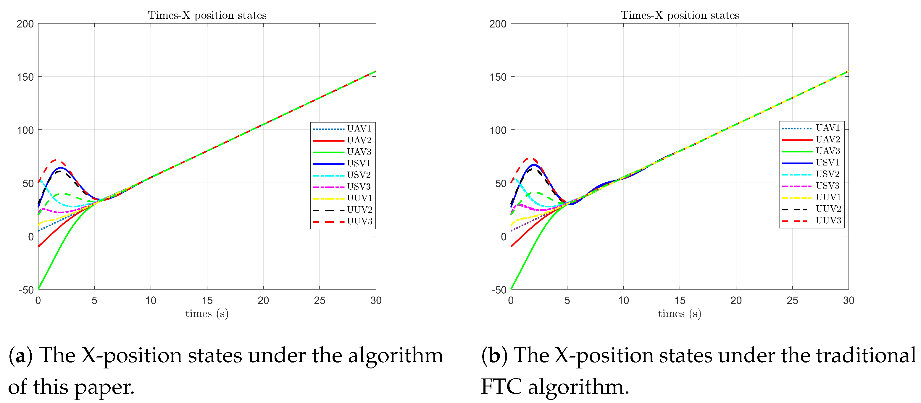
The control protocol proposed in this paper is applied to the leader–follower heterogeneous system composed of UAVs, USVs, and UUVs, and the simulation results are denoted as experimental group (a). The traditional distributed optimal FTC protocol is applied to the same leader–follower HMAS for simulation, and the corresponding results are denoted as control group (b). The two groups of experiments adopt the same parameters, the initial values of each intelligent agent are shown in Table 1. and the comparison of the results is shown in the figure:

As shown in Figure 4, (a) is the simulation diagram of the algorithm proposed in this paper, and (b) is the simulation diagram of the optimal fault-tolerant algorithm. The simulation results indicate that under the algorithm proposed in this paper, the position states of each follower agent on the X-axis first reach agreement with the leader’s state at 5 s and still fluctuate within a small range due to the influence of faults from 5 s to 8 s. In contrast, under the optimal fault-tolerant algorithm, the position states of each follower agent on the X-axis also first reach agreement at 5 s but fluctuate significantly due to the influence of faults from 5 s to 13 s.

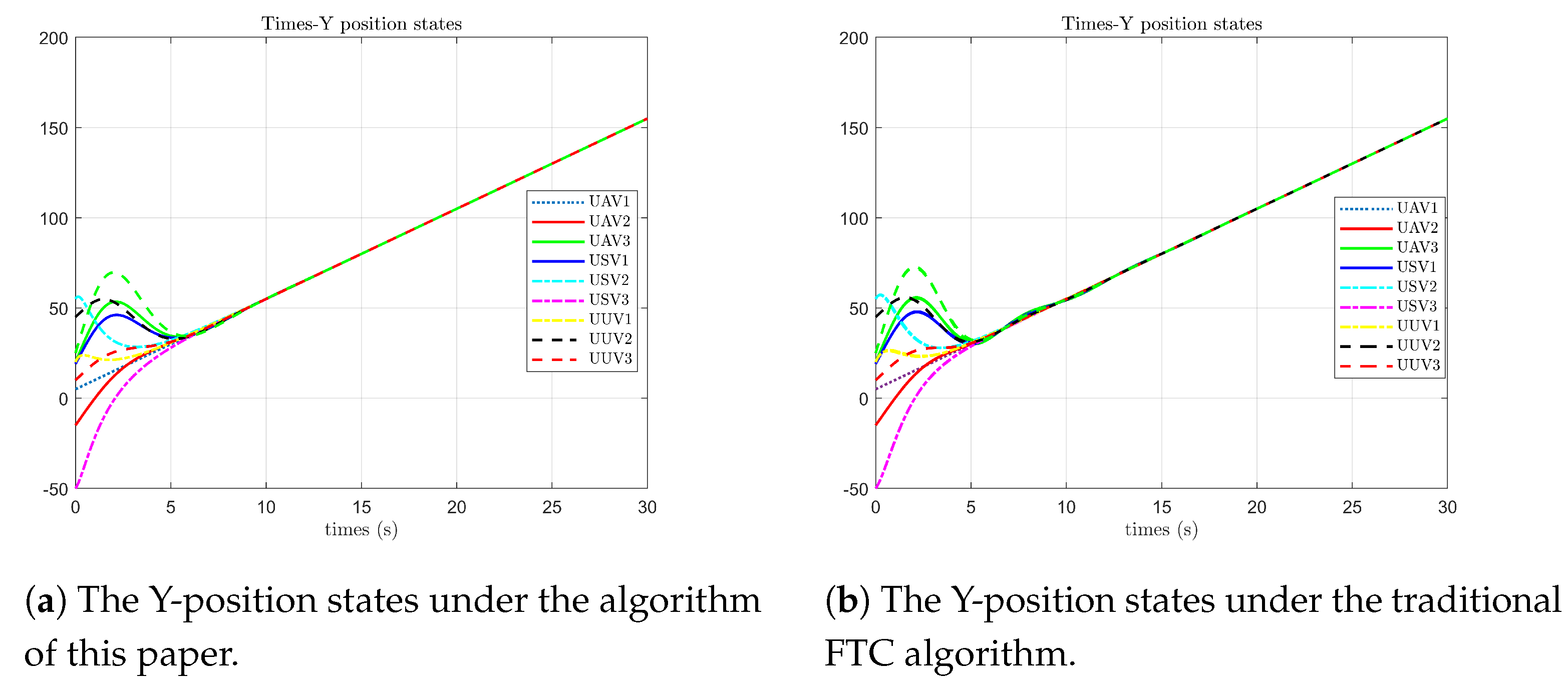
As shown in Figure 5, under the algorithm proposed in this paper, the position states of each follower agent on the Y-axis first reach agreement with the leader’s state at 6 s and still fluctuate within a small range due to the influence of faults from 7 to 8 s. In contrast, under the optimal fault-tolerant algorithm, the position states of each follower agent on the Y-axis first reach agreement at 5 s but fluctuate significantly due to the influence of faults from 7 to 11 s.

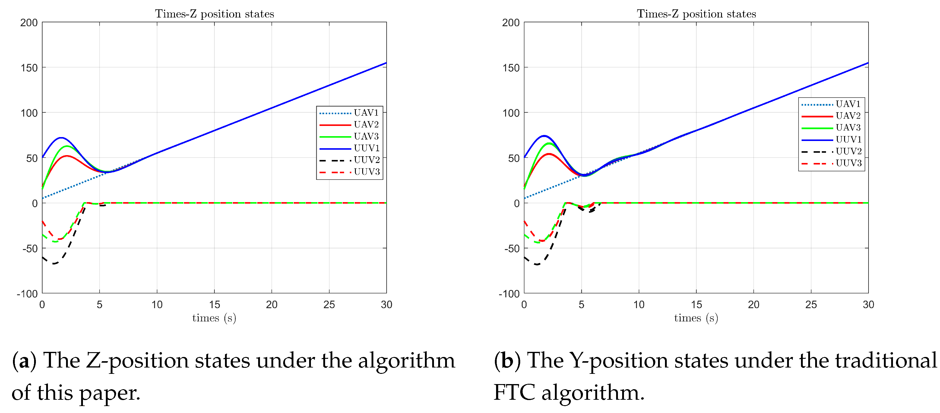
As shown in Figure 6, under the algorithm proposed in this paper, the position state of the follower UAV on the Z-axis reaches agreement with the leader’s state at 6 s. The position state of the follower UUV on the Z-axis is 0 at 4 s (at this time, it is operating at the horizontal plane). The follower UAV still has small-range fluctuations due to the influence of faults from 6 to 7 s, and the follower UUV has small-range fluctuations from 4 to 6 s. In contrast, under the optimal fault-tolerant algorithm, the position state of the follower UAV on the Z-axis reaches agreement with the leader’s state at 5 s. The position state of the follower UUV on the Z-axis is 0 at 4 s. The follower UAV fluctuates significantly due to the influence of faults from 5 to 13 s, and the follower UUV fluctuates significantly from 4 to 7 s.

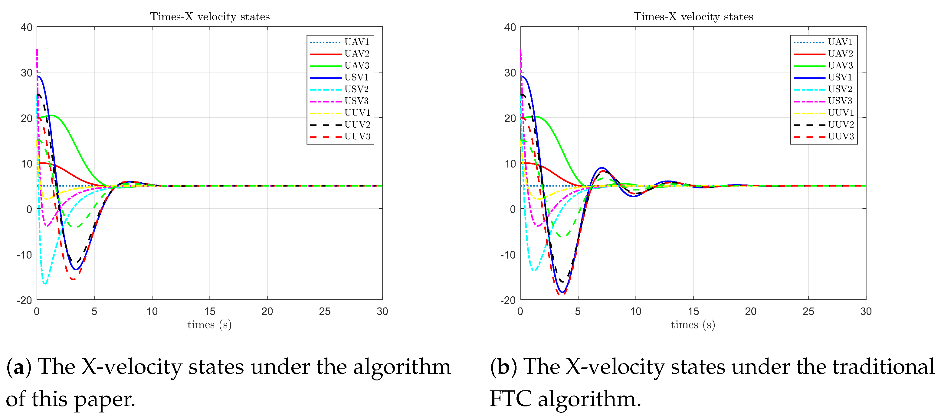
As shown in Figure 7, under the algorithm proposed in this paper, the velocity states of each follower agent on the X-axis first reach agreement with the leader’s state at 7 s. Due to the influence of faults, they still fluctuate within a small range from 7 s to 10 s. In contrast, under the optimal fault-tolerant algorithm, the velocity states of each agent on the X-axis first reach agreement at 6 s. The frequency and amplitude of the fluctuations affected by faults are relatively large, from 6 s to 17 s.

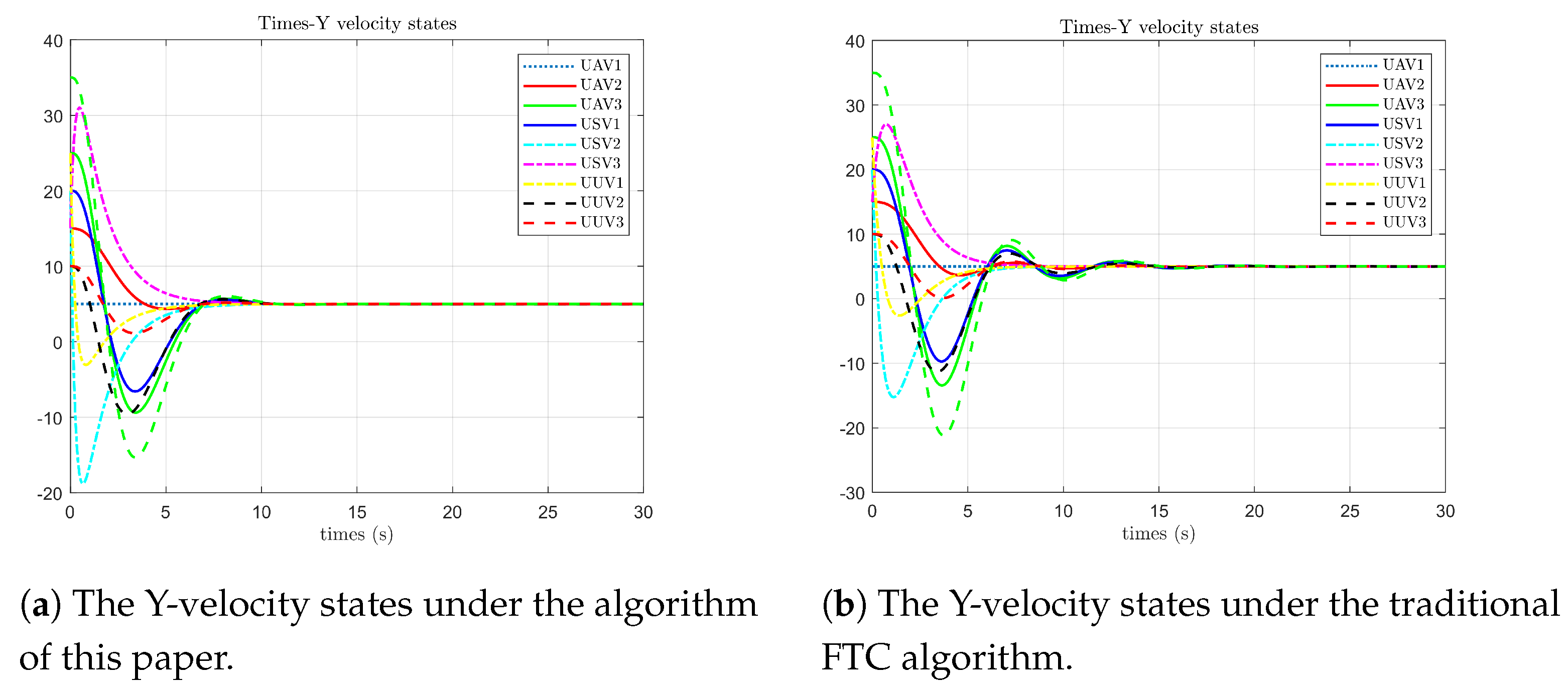
As shown in Figure 8, under the algorithm proposed in this paper, the velocity states of each follower agent on the Y-axis first reach agreement with the leader’s state at 7 s. From 7 to 10 s, they still fluctuate within a small range due to the influence of faults. In contrast, under the optimal fault-tolerant algorithm, the velocity states of each agent on the Y-axis first reach agreement at 6 s. From 6 to 18 s, both the frequency and amplitude of the fluctuations are relatively large due to the influence of faults.

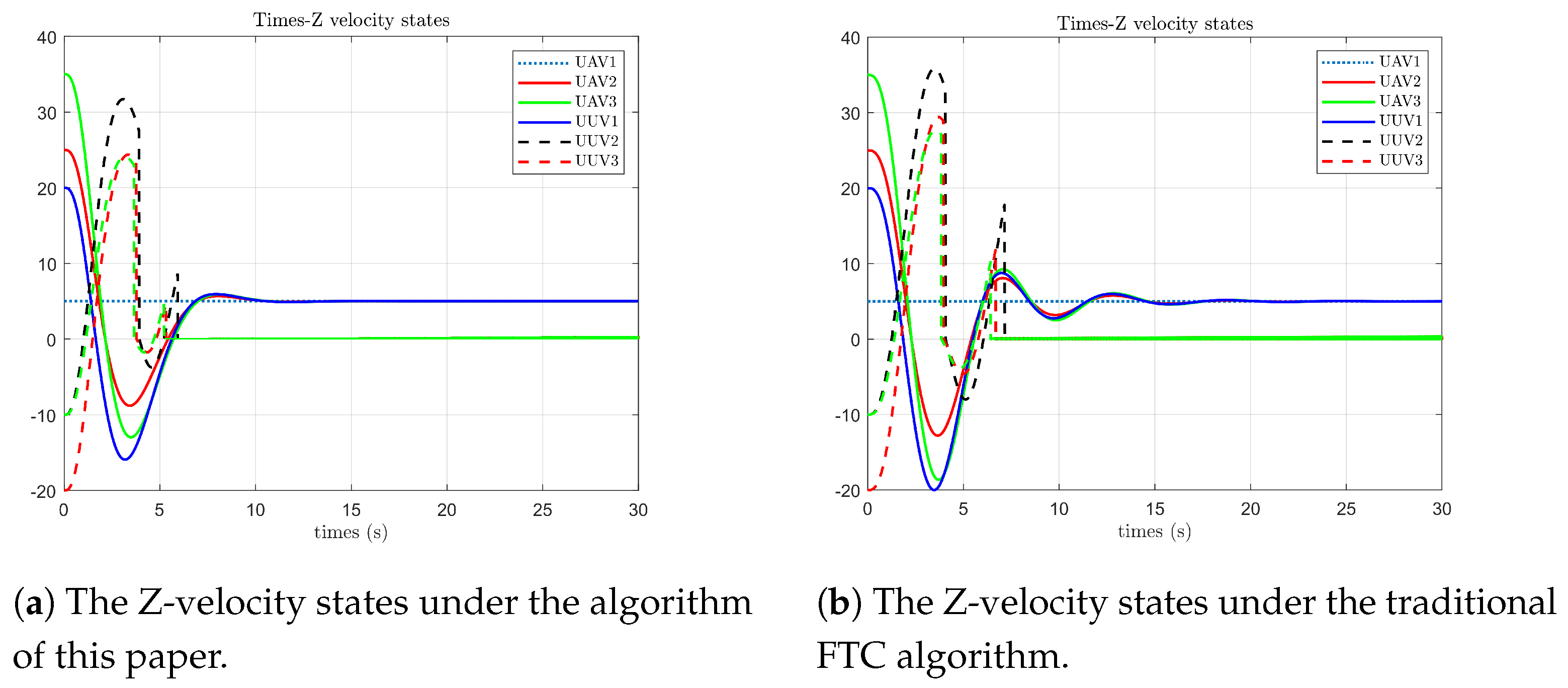
As shown in Figure 9, under the algorithm proposed in this paper, the velocity state of the follower UAV on the Z-axis first reaches agreement with the leader’s state at 6 s. The velocity state of the follower UUV on the Z-axis is 0 at 6 s (at this time, it is operating in the horizontal plane), and the follower UAV still has small-range fluctuations from 6 to 10 s. In contrast, under the optimal fault-tolerant algorithm, the position state of the follower UAV on the Z-axis first reaches agreement with the leader’s state at 6 s. The velocity state of the follower UUV on the Z-axis is 0 at 6 s, and the follower UAV experiences a relatively large number of fluctuations with larger amplitudes from 6 to 18 s due to the influence of faults. Through comparison, it can be seen that when the algorithm proposed in this paper is applied to the aerial–marine surface submarine system, it has better real-time performance. Under the influence of faults, it has fewer state fluctuations, smaller amplitudes, fast convergence, and superior performance.

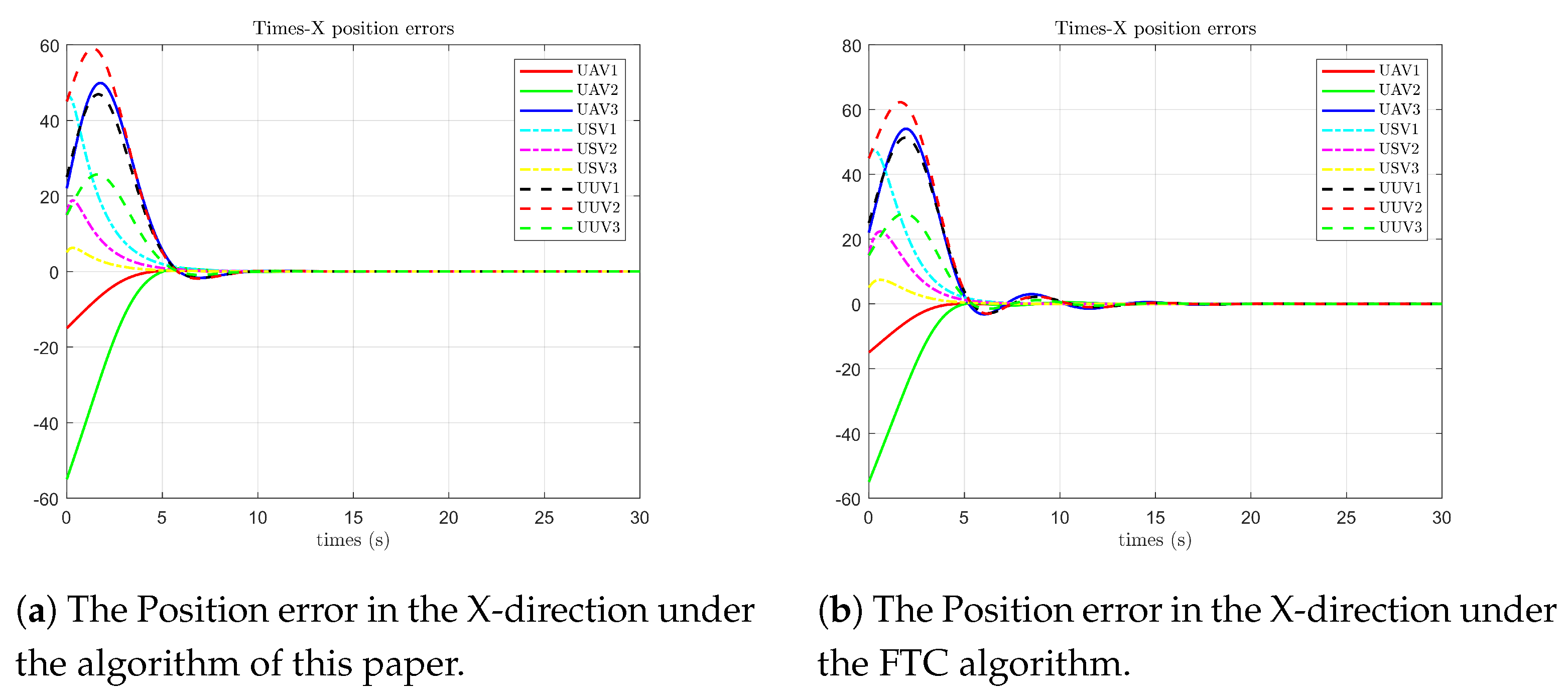
As shown in Figure 10, under the algorithm proposed in this paper, the position error states of each follower agent on the X-axis first reach 0 compared with the leader’s state at 6 s. From 6 to 9 s, due to the influence of faults, there is only one fluctuation, with the maximum peak value being 3. In contrast, under the optimal fault-tolerant algorithm, the position error states of each agent on the X-axis first reach 0 at 5 s. From 5 to 11 s, due to the influence of faults, there are four fluctuations, with the maximum peak value being 8.

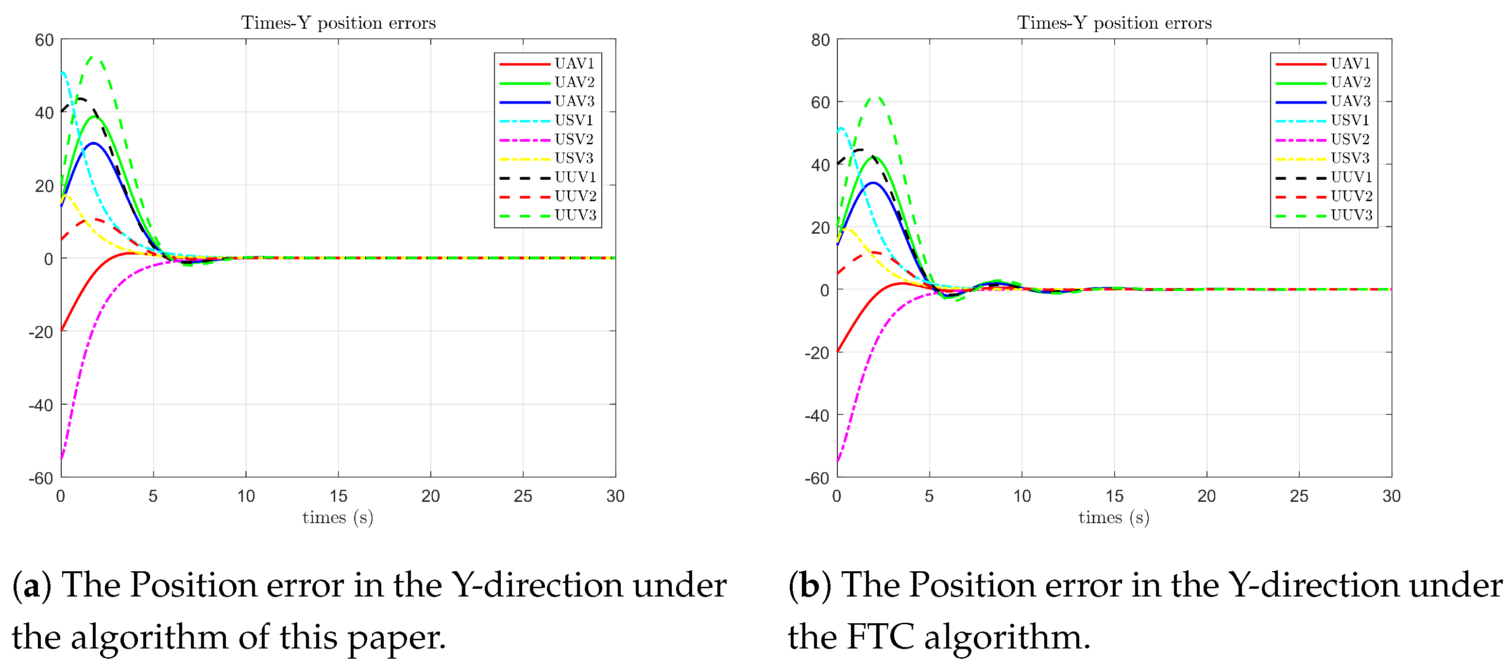
As shown in Figure 11, under the algorithm proposed in this paper, the position error states of each follower agent on the Y-axis first become zero compared with the leader’s state at 6 s. From 6 to 9 s, there is one fluctuation with a maximum peak value of −2 due to the influence of faults. However, under the optimal fault-tolerant algorithm, the position error states of each agent on the X-axis first become zero at 5 s. From 5 to 15 s, affected by the faults, these states fluctuate three times, with a maximum peak value of 5.

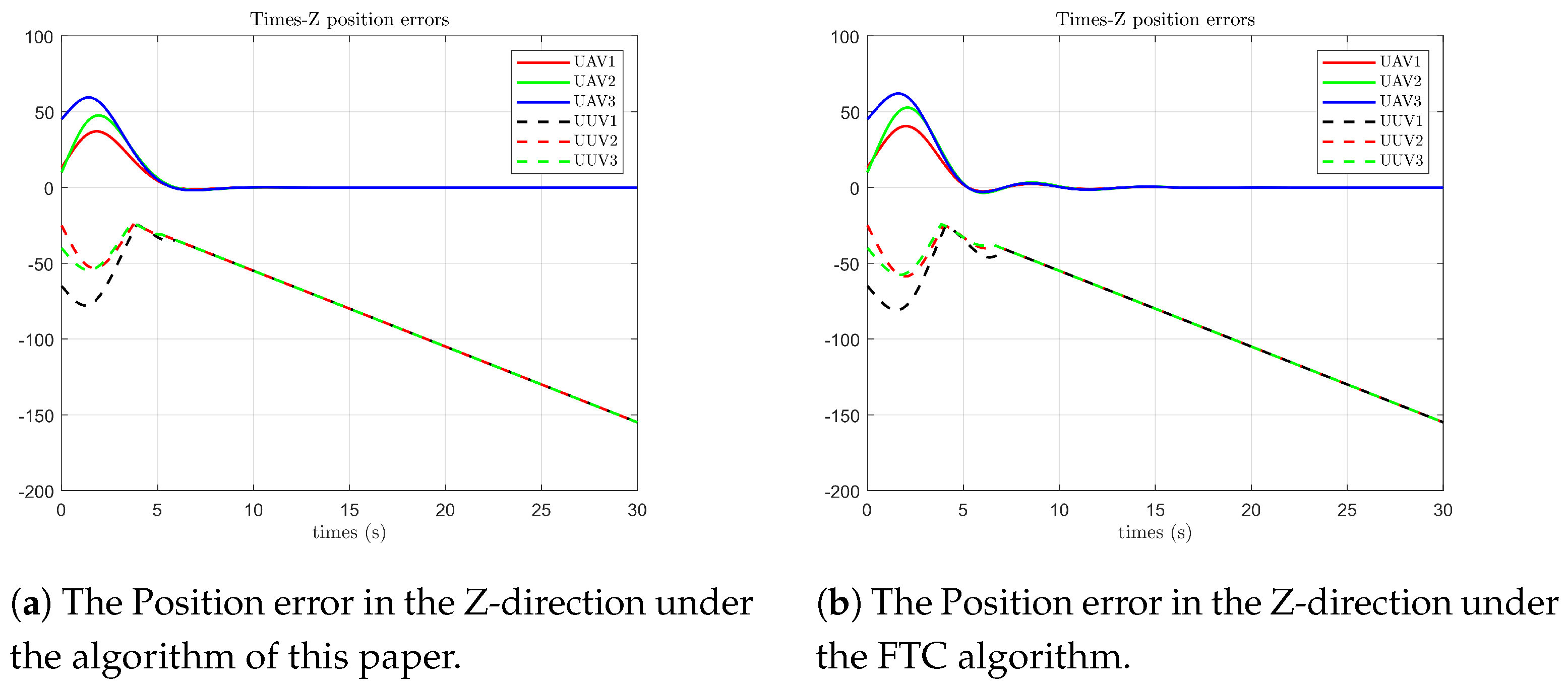
As shown in Figure 12, under the algorithm proposed in this paper, the position error state of the follower UAV on the Z-axis first becomes 0 compared with the leader’s state at 6 s. Affected by the fact that the UUV cannot break away from the water surface, the position error state of the follower UUV on the Z-axis is relatively consistent with that of the leading UAV at 4 s (it is operating on the horizontal plane at this time). The position error state of the follower UAV still has small-scale fluctuations within 5 to 7 s, while there is no fluctuation for the UUV. Under the optimal fault-tolerant algorithm, the position error state of the follower UAV on the Z-axis first becomes 0 compared with the leader’s state at 5 s. The position state of the follower UUV on the Z-axis is first relatively consistent with that of the leading UAV at 4 s. The follower UAV is affected by faults and has more frequent fluctuations with larger amplitudes within 5 to 14 s. The follower UUV is affected by faults and experiences a fluctuation with a relatively large amplitude within 4 to 7 s.

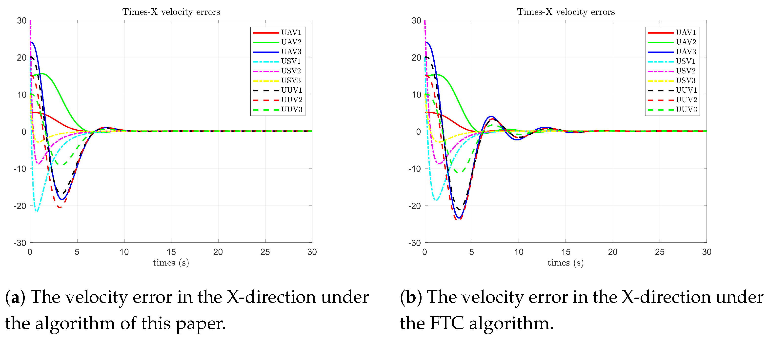
As shown in Figure 13, under the algorithm proposed in this paper, the velocity error states of each follower agent on the X-axis first become 0 compared with the leader’s state at 6 s. From 6 to 10 s, due to the influence of faults, there is still one fluctuation, with the maximum peak value being 2. However, under the optimal fault-tolerant algorithm, the velocity error states of each follower agent on the X-axis first become 0 at 6 s. From 5 to 18 s, affected by the faults, the states fluctuate four times, with the maximum peak value being 5.

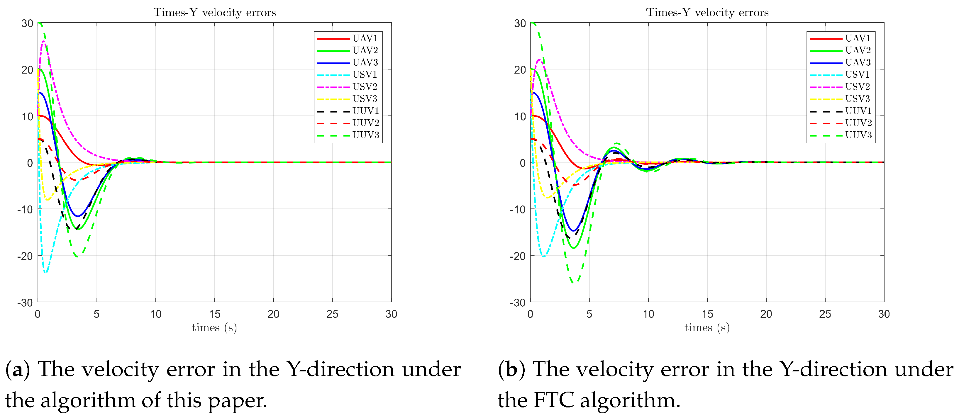
As shown in Figure 14, under the algorithm proposed in this paper, the velocity error states of each follower agent on the Y-axis first become 0 compared with the leader’s state at 6 s. From 6 to 9 s, due to the influence of faults, there is one fluctuation, with the maximum peak value being 1.5. However, under the optimal fault-tolerant algorithm, the velocity error states of each agent on the Y-axis first become 0 at 6 s. From 5 to 15 s, affected by the faults, the states fluctuate three times, with the maximum peak value being 4.

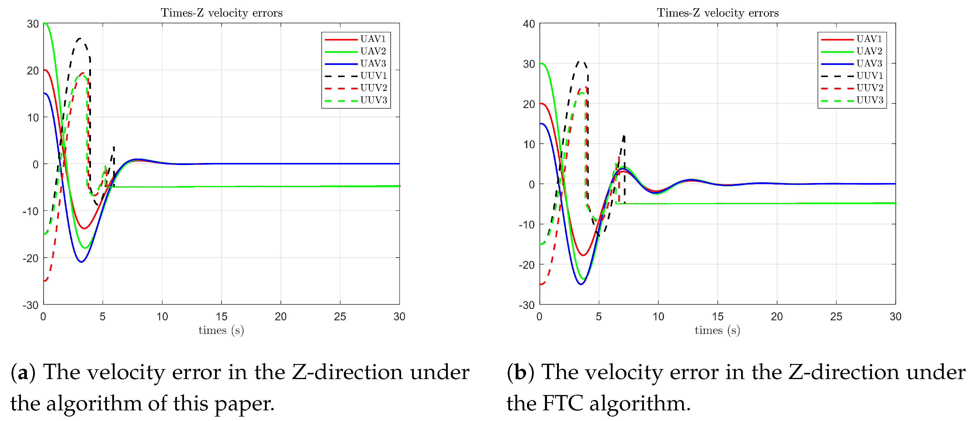
As shown in Figure 15, it can be known from the simulation that under the algorithm in this paper, the velocity error state of the follower UAV on the Z-axis first becomes 0 compared with the leader’s state at 7 s. Affected by the fact that the UUV cannot break away from the water surface, the velocity state of the follower UUV on the Z-axis is relatively consistent with that of the leading UAV at 6 s (it is operating on the horizontal plane at this time), and the follower UAV still has small-scale fluctuations within 7 to 9 s. Under the optimal fault-tolerant algorithm, the velocity error state of the follower UAV on the Z-axis first becomes 0 compared with the leader’s state at 7 s. The velocity error state of the follower UUV on the Z-axis is relatively consistent with that of the leading UAV at 8 s, and the follower UAV is affected by faults and has more frequent fluctuations with larger amplitudes within 7 to 19 s.

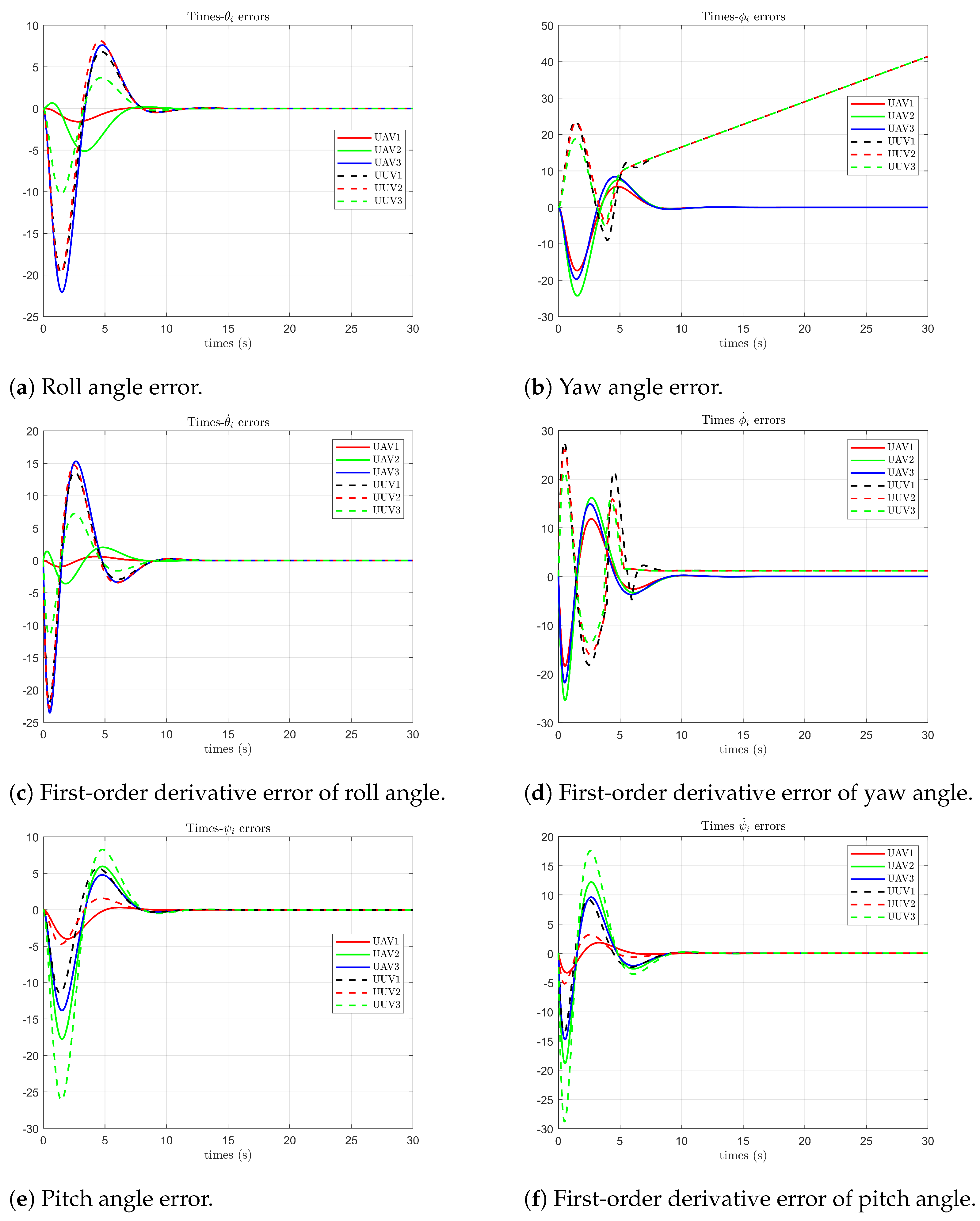
Figure 16 demonstrate that the roll angle errors, pitch angle errors, first-order derivative errors of the roll angle, and first-order derivative errors of the pitch angle of UAVs and UUVs relative to the leader UAV exhibit fluctuations at 10 s due to fault impacts, and gradually stabilize after 15 s. The yaw angle errors and first-order derivative errors of the yaw angle between UUVs, UAVs, and the leader UAV remain oscillatory at 10 s under the combined effects of marine surface constraints and faults, achieving relative stability after 15 s.

Figure 17 illustrates that in a three-dimensional space, UAVs maneuver above the horizontal plane, USVs navigate on the horizontal plane, and UUVs operate submarines. Constrained by the respective dynamic models, only the follower UAVs can achieve full 3D consensus (X, Y, and Z directions) with the leader UAV. The follower USVs and UUVs will maintain their operations on the marine surface and submarine domains beneath the leader UAV.

Faults are incorporated into the distributed consensus control framework of multi-agent systems. The parameters employed in this experimental setup are consistent with those detailed in the preceding sections. The corresponding experimental outcomes are visually presented in the subsequent figure:

As depicted in Figure 18, when faults occur, the position errors along the X, Y, and Z-axes and the velocity errors along the X, Y, and Z-axes for each intelligent agent exhibit multiple significant fluctuations. The most pronounced amplitude fluctuation resulting from the faults is observed in the velocity component along the X-axis, where a drastic fluctuation with an amplitude of 15 is registered. Eventually, the error states of all the intelligent agents converge and achieve consistency with those of the leader agent.

The second set of experimental scenarios is selected to simulate the algorithm proposed in this paper, and the fault matrix is as follows:

$$P_{A1}=\left[\begin{array}{ccc}0.5{\sin }^2\left(t\right)& 0& 0\\ 0& 0.7{\cos }^2\left(t\right)+0.5& 0\\ 0& 0& 1\end{array}\right],P_{A2}=\left[\begin{array}{ccc}{\sin }^2\left(t\right)& 0& 0\\ 0& 0.5\cos \left(t\right)+0.5sin\left(t\right)& 0\\ 0& 0& {\left({\displaystyle \frac{1}{2}}\right)}^t\end{array}\right],$$

$$P_{A3}=\left[\begin{array}{ccc}0.5& 0& 0\\ 0& {\left({\displaystyle \frac{1}{4}}\right)}^t& 0\\ 0& 0& 1\end{array}\right],P_{S1}=\left[\begin{array}{cc}1& 0\\ 0& {\left({\displaystyle \frac{1}{3}}\right)}^t\end{array}\right],P_{S2}=\left[\begin{array}{cc}{\cos }^2\left(t\right)& 0\\ 0& 0.1+0.5{\sin }^3\left(\mathrm{t}\right)\end{array}\right],$$

$$P_{S3}=\left[\begin{array}{cc}{\left({\displaystyle \frac{1}{3}}\right)}^t& 0\\ 0& 1\end{array}\right]P_{U1}=\left[\begin{array}{ccc}{\displaystyle \frac{0.7}{t}}& 0& 0\\ 0& 0.3{\cos }^4\left(t\right)+0.7& 0\\ 0& 0& 1\end{array}\right],$$

$$P_{U2}=\left[\begin{array}{ccc}1& 0& 0\\ 0& 0.2\sin \left(t\right)& 0\\ 0& 0& 0.6\end{array}\right],P_{U3}=\left[\begin{array}{ccc}{\displaystyle \frac{0.3}{t}}& 0& 0\\ 0& 1& 0\\ 0& 0& 0.3\cos \left(\mathrm{t}\right)+0.7\sin \left(\mathrm{t}\right)\end{array}\right]$$

As shown in Figure 19, and affected by the fault, the position error of each agent in the X-direction experiences a fluctuation with a maximum peak of −1.2 between 6 and 8 s, and then the error with the leader becomes 0.The position error of each agent in the Y-direction experiences a fluctuation with a maximum peak of −0.8 between 6 and 8 s, and then the error with the leader becomes 0. There is almost no fluctuation in the error of each agent in the Z-direction. The velocity error of each agent in the X-direction experiences a fluctuation with a maximum peak of 1.5 between 6 and 8 s, and then the error with the leader becomes 0. The velocity error of each agent in the Y-direction experiences a fluctuation with a maximum peak of 0.9 between 6 and 8 s, and then the error with the leader becomes 0. The velocity error of the UAV in the Z-direction experiences a fluctuation with a maximum peak of 0.4 between 6 and 8 s, and then the error with the leader becomes 0, while the UUV is hardly affected by the fault.

5. Conclusions

This paper analyzes the dynamic models of UAVs, USVs, and UUVs and establishes an HMAS. An optimal FTC control protocol is designed, which effectively solves the FTC control problem of the aerial–marine surface submarine HMAS under partial actuator failures and interruption faults and ensures that the states of each follower agent can reach an agreement with that of the leader agent in case of failures. Subsequently, the asymptotic stability of the system is proven by using Lyapunov stability theory, and the effectiveness of the control protocol and the feasibility of the control strategy are further verified through comparative simulation experiments.

The complex marine environment poses a great challenge to the reliability of sensors, actuators, and other components. Fault diagnosis and tolerance can only implement corresponding fault-tolerance measures under conditions such as stable and reliable communication. As the complexity of the system increases, the complexity of the fault-tolerance methods also keeps rising, which will lead to a decrease in the fault-tolerance processing speed of the system. Advanced fault diagnosis and fault-tolerance methods have become a research hotspot, and at the same time, important topics such as input saturation and formation control have emerged. In future work, we will be committed to the research of more advanced fault-tolerance solutions. For example, integrating the event-triggered mechanism into fault tolerance can further improve the efficiency of system fault tolerance.

References

1. Tanner, H.G.; Jadbabaie, A.; Pappas, G.J. Stable flocking of mobile agents, Part I: Fixed topology. In Proceedings of the 42nd IEEE International Conference on Decision and Control (IEEE Cat. No. 03CH37475), Maui, HI, USA, 9–12 December 2003; Volume 2, pp. 2010–2015. [Google Scholar]
2. Boschetti, G.; Bottin, M.; Faccio, M.; Minto, R. Multi-robot multi-operator collaborative assembly systems: A performance evaluation model. J. Intell. Manuf. 2021, 32, 1455–1470. [Google Scholar] [CrossRef]
3. Wang, F.Y.; Lin, Y.; Ioannou, P.A.; Vlacic, L.; Liu, X.; Eskandarian, A.; Lv, Y.; Na, X.; Cebon, D.; Ma, J.; et al. Transportation 5.0: The DAO to safe, secure, and sustainable intelligent transportation systems. IEEE Trans. Intell. Transp. Syst. 2023, 24, 10262–10278. [Google Scholar] [CrossRef]
4. Wang, L.; Zhu, D.; Pang, W.; Zhang, Y. A survey of underwater search for multi-target using Multi-AUV: Task allocation, path planning, and formation control. Ocean Eng. 2023, 278, 114393. [Google Scholar] [CrossRef]
5. Fazlollahtabar, H.; Hassanli, S. Hybrid cost and time path planning for multiple autonomous guided vehicles. Appl. Intell. 2018, 48, 482–498. [Google Scholar] [CrossRef]
6. Cai, M.; He, X.; Zhou, D. Self-healing fault-tolerant control for high-order fully actuated systems against sensor faults: A redundancy framework. IEEE Trans. Cybern. 2023, 54, 2628–2640. [Google Scholar] [CrossRef]
7. He, W.; Xu, W.; Ge, X.; Han, Q.L.; Du, W.; Qian, F. Secure control of multiagent systems against malicious attacks: A brief survey. IEEE Trans. Ind. Inform. 2021, 18, 3595–3608. [Google Scholar] [CrossRef]
8. Wu, X.; Zhao, N.; Ding, S.; Wang, H.; Zhao, X. Distributed event-triggered output-feedback time-varying formation fault-tolerant control for nonlinear multi-agent systems. IEEE Trans. Autom. Sci. Eng. 2024, 22, 3810–3821. [Google Scholar] [CrossRef]
9. Davoodi, M.; Meskin, N.; Khorasani, K. Simultaneous fault detection and consensus control design for a network of multi-agent systems. Automatica 2016, 66, 185–194. [Google Scholar] [CrossRef]
10. Ingimundarson, A.; Bravo, J.M.; Puig, V.; Alamo, T.; Guerra, P. Robust fault detection using zonotope-based set-membership consistency test. Int. J. Adapt. Control Signal Process. 2009, 23, 311–330. [Google Scholar] [CrossRef]
11. Zhao, L.; Zhao, F.; Che, W.W. Distributed adaptive fuzzy fault-tolerant control for multi-agent systems with node faults and denial-of-service attacks. Inf. Sci. 2023, 631, 385–395. [Google Scholar] [CrossRef]
12. Cui, G.F.; Wu, L.B.; Wu, M. Adaptive event-triggered fault-tolerant control for leader-following consensus of multi-agent systems. Int. J. Syst. Sci. 2024, 55, 3291–3303. [Google Scholar] [CrossRef]
13. Zhang, P.; Xue, H.; Gao, S. Multi-agent fault-tolerant control based on distributed adaptive consensus. IEEE Access 2019, 7, 135882–135895. [Google Scholar] [CrossRef]
14. Liu, F.; Hua, Y.; Dong, X.; Li, Q.; Ren, Z. Adaptive fault-tolerant time-varying formation tracking for multi-agent systems under actuator failure and input saturation. ISA Trans. 2020, 104, 145–153. [Google Scholar] [CrossRef]
15. Liu, F.; Ma, Z.; Mu, B.; Duan, C.; Chen, R.; Qin, Y.; Pu, H.; Luo, J. Review on fault-tolerant control of unmanned underwater vehicles. Ocean Eng. 2023, 285, 115471. [Google Scholar] [CrossRef]
16. Li, C.; Luo, K.; Yang, L.; Li, S.; Wang, H.; Zhang, X.; Liao, Z. A zero-shot fault detection method for UAV sensors based on a novel CVAE-GAN model. IEEE Sens. J. 2024, 24, 23239–23254. [Google Scholar] [CrossRef]
17. Zhang, G.; Chu, S.; Zhang, W.; Liu, C. Adaptive neural fault-tolerant control for USV with the output-based triggering approach. IEEE Trans. Veh. Technol. 2022, 71, 6948–6957. [Google Scholar] [CrossRef]
18. Wang, X. Active fault tolerant control for unmanned underwater vehicle with sensor faults. IEEE Trans. Instrum. Meas. 2020, 69, 9485–9495. [Google Scholar] [CrossRef]
19. Wei, W.; Wang, J.; Fang, Z.; Chen, J.; Ren, Y.; Dong, Y. 3U: Joint design of UAV-USV-UUV networks for cooperative target hunting. IEEE Trans. Veh. Technol. 2022, 72, 4085–4090. [Google Scholar] [CrossRef]
20. Kang, J.; Choi, K. Development of an artificial neural network control allocation algorithm for small tailless aircraft based on dynamic allocation method. Int. J. Aeronaut. Space Sci. 2022, 23, 363–378. [Google Scholar] [CrossRef]
21. Chen, Y.; Hao, S.; Gao, J.; Wang, J.; Li, L. Fault-Tolerant Model Predictive Control for Autonomous Underwater Vehicles Considering Unknown Disturbances. J. Mar. Sci. Eng. 2025, 13, 171. [Google Scholar] [CrossRef]
22. Gong, H.; Er, M.J.; Liu, Y. Fuzzy adaptive optimal fault-tolerant trajectory tracking control for underactuated AUVs with input saturation. Ocean Eng. 2024, 311, 118940. [Google Scholar] [CrossRef]
23. Chen, G.; Dong, J. Approximate optimal adaptive prescribed performance fault-tolerant control for autonomous underwater vehicle based on self-organizing neural networks. IEEE Trans. Veh. Technol. 2024, 73, 9776–9785. [Google Scholar] [CrossRef]
24. Härkegård, O.; Glad, S.T. Resolving actuator redundancy—Optimal control vs. control allocation. Automatica 2005, 41, 137–144. [Google Scholar] [CrossRef]
25. Engwerda, J. LQ Dynamic Optimization and Differential Games; John Wiley & Sons: Hoboken, NJ, USA, 2005. [Google Scholar]
26. Lai, L.C.; Yang, C.C.; Wu, C.J. Time-optimal control of a hovering quad-rotor helicopter. J. Intell. Robot. Syst. 2006, 45, 115–135. [Google Scholar] [CrossRef]
27. Xie, W.; Ma, B.; Fernando, T.; Iu, H.H.C. A new formation control of multiple underactuated surface vessels. Int. J. Control 2018, 91, 1011–1022. [Google Scholar] [CrossRef]
28. Zhang, W.; Zeng, J.; Yan, Z.; Wei, S.; Zhang, J.; Yang, Z. Consensus control of multiple AUVs recovery system under switching topologies and time delays. IEEE Access 2019, 7, 119965–119980. [Google Scholar] [CrossRef]
Figure 1. UAV.
Jmse 13 00878 g001
Figure 2. USV.
Jmse 13 00878 g002
Figure 3. UUV.
Jmse 13 00878 g003
Figure 4. Times-position states.
Jmse 13 00878 g004
Figure 5. Times-Y position states.
Jmse 13 00878 g005
Figure 6. Times-Z position states.
Jmse 13 00878 g006
Figure 7. Times-X velocity states.
Jmse 13 00878 g007
Figure 8. Times-Y velocity states.
Jmse 13 00878 g008
Figure 9. Times-Z velocity states.
Jmse 13 00878 g009
Figure 10. Position error in the X-direction.
Jmse 13 00878 g010
Figure 11. Position error in the Y-direction.
Jmse 13 00878 g011
Figure 12. Position error in the Z-direction.
Jmse 13 00878 g012
Figure 13. Velocity error in the X-direction.
Jmse 13 00878 g013
Figure 14. Velocity error in the Y-direction.
Jmse 13 00878 g014
Figure 15. Velocity error in the Z-direction.
Jmse 13 00878 g015
Figure 16. Attitude angle error diagram under the algorithm of this paper.
Jmse 13 00878 g016
Figure 17. Heterogeneous Fault-Tolerant Consensus Spatial States.
Jmse 13 00878 g017
Figure 18. State errors of velocity and position under the consistency algorithm.
Jmse 13 00878 g018
Figure 19. State errors of velocity and position under the algorithm of this paper.
Jmse 13 00878 g019aJmse 13 00878 g019b