Article

Simplified Model Characterization and Control of an Unmanned Surface Vehicle

by
Aldo Lovo-Ayala
1,
Roosvel Soto-Diaz
2,*,
Carlos Andres Gutierrez-Martinez
1,
Jose Fernando Jimenez-Vargas
3,
Javier Jiménez-Cabas
4 and
Jose Escorcía-Gutierrez
4,*
1
Escuela Naval de Cadetes “Almirante Padilla” (ENAP), Cartagena de Indias 130001, Colombia
2
Biomedical Engineering Program, Universidad Simón Bolívar, Barranquilla 080002, Colombia
3
Department of Electrical and Electronic Engineering, Universidad de Los Andes, Bogotá 111711, Colombia
4
Department of Computational Science and Electronics, Universidad de la Costa (CUC), Barranquilla 080002, Colombia
*
Authors to whom correspondence should be addressed.
J. Mar. Sci. Eng. 2025, 13(4), 813; https://doi.org/10.3390/jmse13040813
Submission received: 14 March 2025 / Revised: 13 April 2025 / Accepted: 16 April 2025 / Published: 18 April 2025

Abstract

:
This study presents the modeling and control of the unmanned surface vehicle (USV) SABALO. Two models were built, one based on a transfer function matrix and another based on state variables, and from these models, two control strategies were developed. The first strategy is based on independent Proportional-Integral/Proportional-Derivative (PI/PD) controllers complemented by a decoupling system, and the second strategy is based on state variable feedback. The two control strategies were evaluated and contrasted. Results demonstrated that the decoupler effectively eliminated variable interaction, enhancing stability in straight trajectories and directional changes. Meanwhile, state feedback control demonstrated markedly faster response times and superior precision, accompanied by higher energy consumption. The study concludes that both strategies are effective, but their suitability depends on the mission. The decoupler could be ideal for energy-efficient, long-duration operations, while state feedback could be appropriate for dynamic environments requiring rapid maneuvers.

1. Introduction

An Unmanned Surface Vehicle (USV) is an autonomous craft that operates on the surface of a body of water without any personnel onboard. They can be remotely operated by an operator positioned on land or another vessel. This capability ensures a primary line of defense and facilitates the inspection of other ships, all while keeping manned boats at a safe distance to minimize unnecessary risks. The evolution of USVs since their inception in the 1960s has significantly advanced maritime operations. Initially, USVs were designed to perform basic remote-controlled tasks; however, with the integration of cutting-edge technologies, they can perform military and scientific research missions, such as monitoring marine/river areas, conducting oceanographic measurements, measuring river water flow, mapping, and detecting riverbank lines [1,2,3,4,5]. As their applications have diversified and become more complex, the need for accurate modeling and control strategies has grown significantly.
Accurate dynamic modeling and parameter identification have become essential for enhancing the precision and robustness of USV control systems. A number of approaches have been proposed to enhance these aspects. For instance, Abrougui et al. developed a comprehensive mathematical model with three degrees of freedom (DOF), achieving effective parameter identification through sea trials and significantly improving the autopilot’s accuracy for waypoint tracking and route following [6]. Setiawan et al. presented a detailed dynamic modeling approach for USVs employing the nonlinear Levenberg–Marquardt method, which facilitated reliable parameter estimation validated through real-time experiments [7]. Furthermore, Zhang and Ren [8] introduced a non-parametric multi-output Gaussian process (MOGP) learning method, capable of effectively capturing complex nonlinear interactions across multiple DOFs, thus providing enhanced robustness and computational efficiency. In a similar vein, Xu et al. [9] employed a combination of least square support vector machines (LS-SVMs) and a cuckoo search optimization algorithm to achieve accurate parameter identification, underscoring the efficacy of this approach in comparison to traditional methods. Moreover, Zhong et al. [10] employed a nonlinear multi-innovation least-squares (NMILS) algorithm, further improving the accuracy of parameter identification and ensuring robust control performance through finite-time sliding mode control (FTSMC), validating their methods in simulation environments. Ma et al. [11] proposed a multi-model predictive control strategy to handle path-following tasks under wide-range speed variations, enhancing control stability and adaptability in dynamic marine environments. These methodologies significantly contribute to the field; however, their application in real life is limited due to the complexity of some of the proposed models.
In addition, regardless of their purposes or missions, USVs require an effective maneuvering controller to ensure successful operation throughout their missions. Many works have been developed focusing on USV control, as shown in Table 1. The majority of these strategies rely on complex methodologies, including predictive control, adaptive control, artificial intelligence (AI), deep learning (DL), and nonlinear control strategies [12,13,14]. In recent years, machine learning techniques, including deep reinforcement learning (DRL) and neural network-based models, have become increasingly prevalent [13]. These techniques have demonstrated remarkable adaptability and self-learning capabilities in complex and dynamic environments. For instance, Zhao et al. [8] proposed a DRL-based path-following method, which showed improved convergence but required high computational resources to handle continuous action spaces. Similarly, Wang et al. [12] developed an optimal path-following controller for USVs using reinforcement learning, but its reliance on extensive training data limited its real-world adaptability.
The recent literature has also emphasized the importance of the accurate modeling and control of USVs. Several studies have proposed a novel cost control method guaranteed by network-based modeling and sampling for USVs subjected to stochastic cyber-attacks, addressing the robustness and performance degradation problems caused by network instabilities [15]. Furthermore, other research has introduced a hybrid adaptive dynamic programming approach for the optimal control of USV tracking, which has been shown to significantly improve trajectory tracking performance and minimize energy consumption [16]. Furthermore, an adaptive formation control strategy was proposed for USV obstacle avoidance with asymmetric input saturation, demonstrating improved maneuverability and operational safety in complex marine environments [17]. Furthermore, other authors have presented a multi-model predictive control strategy for USV trajectory tracking over various velocity variations. This approach demonstrated significant robustness and adaptability to dynamic marine conditions, effectively maintaining trajectory accuracy despite wide speed variations [11]. These novel approaches reflect the growing trend of integrating advanced modeling techniques with robust control strategies to address the challenges posed by environmental disturbances, cyber-attacks, and operational uncertainties.
Nevertheless, despite the advantages of machine learning-based methods, they present inherent limitations that hinder their practical applicability in real-time marine operations. A primary challenge is the necessity of substantial volumes of high-quality data for practical model training and generalization. Additionally, the parameter tuning process can be computationally expensive and sensitive to variations in environmental conditions, leading to performance degradation when encountering unfamiliar scenarios. Furthermore, the interpretability of neural network-based models is a matter of concern, as it complicates the implementation of safety-critical applications, where transparency and predictability are essential [11,15,16].
Thus, accurate modeling integrated with robust control strategies is essential to achieving reliable and efficient USV operations. The combination of modeling and control facilitates trajectory optimization and addresses environmental disturbances and operational stability challenges. Although these strategies improve trajectory-tracking accuracy, they often suffer from high implementation complexity, which makes them impractical for real-time marine operations. In contrast, our approach optimizes USV trajectory tracking by leveraging a more computationally efficient strategy while maintaining adaptability to environmental disturbances. Our method balances accuracy and real-time feasibility by reducing the dependency on extensive offline training and computationally intensive deep learning architectures, ensuring robust performance without incurring excessive computational costs. To achieve this, the proposed work develops control strategies based on simple models that effectively capture the dynamic behavior of USVs. Two models with two inputs and two outputs were constructed as follows: one based on a transfer function matrix and another using state variables. From these, two control strategies were implemented. The first utilizes independent Proportional-Integral/Proportional-Derivative (PI/PD) controllers with a decoupling system to mitigate possible inter-loop interactions. The second strategy employs state feedback control with an integrated state estimator to address sensor limitations and enhance overall system observability.
The paper is organized as follows: Section Table 1 contextualizes the study within the existing body of knowledge. Section 2 provides detailed insights into the USV’s design and hardware specifications. Section 3 details aspects such as the input and output variables of the system, the experiments carried out to generate the data, the identified models, and the results of the validations of such models. Section 4 evaluates two control strategies, an independent loop control with a decoupler and state feedback control, supported by performance metrics and simulations. Finally, the investigation concludes with Section 5 and Section 6, summarizing the findings and highlighting the most significant outcomes.
Table 1. Summary of related works on USV modeling and control strategies.
TitleAuthorsMethodsResultsContributionsAdvantages and Disadvantages
Adaptive Control Scheme for USV Trajectory-Tracking Under Complex Environmental Disturbances via Deep Reinforcement LearningYuan Zhou et al. [13]Deep Reinforcement Learning (TD3) for trajectory trackingImproved tracking under dynamic conditions; enhanced learning stabilityRobust DRL-based control for USVs, superior to MPCA: High adaptability to disturbances; D: High computational cost
Network-Based Modeling and Sampling Guaranteed Cost Control for Unmanned Surface Vehicle Systems Under Stochastic Cyber-AttacksKui Ding and Quanxin Zhu [15]DStochastic composite system with Lyapunov functionsStabilizes USVs under cyber-attacks with controlled costIntroduces a cost-effective control method for cyber-attack scenariosA: Ensures system stability under uncertain conditions; D: Relies on precise system modeling
Multi-Model Predictive Control Strategy for Path-Following of Unmanned Surface Vehicles in Wide-Range Speed VariationsYingkai Ma et al. [11]Multi-model predictive control (MPC) with LMI-based robust control and adaptive LOS guidanceImproved path-following accuracy and robustness under speed variationsEnhanced USV maneuverability and control efficiency in dynamic speed conditionsA: Higher efficiency in dynamic speed conditions; D: Computational complexity and need for precise models
Investigation of Wind Effects on UAV Adaptive PID Based MPC Control SystemA. S. Martinez Leon et al. [18]Adaptive PID-based MPC control strategyImproved UAV stabilization and positioning accuracy in the presence of wind disturbancesEnhanced remote surveillance missions along coastlines; insights into wind effects on UAV controlA: Effective for coastal surveillance missions; D: Limited to UAV applications, not directly applicable to USVs
Adaptive Formation Control for Obstacle Avoidance in USVsHu Yancai, Liu Yang, et al. [17]RBF neural networks and APF method for formation controlEffective obstacle avoidance while maintaining formationProvides robust formation control in dynamic environmentsA: Handles complex obstacle avoidance; D: May struggle with numerous obstacles or extreme conditions
Safe Autonomy for Uncrewed Surface Vehicles Using Adaptive Control and Reachability AnalysisKaran Mahesh et al. [19]Model Reference Adaptive Control (MRAC) with Moving Horizon Estimator (MHE) for real-time disturbance estimation45–81% reduction in position error compared to PID; enhanced real-time safety certificationImproved USV stability in dynamic environments and robust real-time safety verificationA: Improved stability and safety verification in dynamic environments; D: High implementation complexity and computational requirements
Evolution of Algorithms and Applications for Unmanned Surface Vehicles in the Context of Small Craft: A Systematic ReviewLuis Castano-Londono et al. [20]Systematic literature review using PRISMA and bibliometric analysisIdentified 387 studies on USV applications and algorithm trendsProvided a comprehensive mapping of USV research, focusing on small craft applicationsA: Comprehensive mapping of USV research; D: Does not propose new methods, only a review
Hybrid Adaptive Dynamic Programming for Optimal Tracking Control of USVsShan Xue, Ning Zhao, et al. [16]Integration of IRL and DED mechanismsReduced communication overhead and improved trackingReduces model dependency in tracking controlA: Efficient learning with minimal data transmission; D: Requires significant computational resources
A Model Predictive Control Approach for USV Autonomous Cruising via Disturbance LearningMaotong Cheng et al. [14]Learning-based MPC, augmented by LSTM residual modelImproved course-keeping under disturbances; LSTM eliminates model mismatchImproved hydrodynamics modeling for USVs through MPC and LSTMA: Enhanced hydrodynamic modeling; D: Dependency on historical data for LSTM training
Disturbance Estimation and Rejection in an Underwater Autonomous VehicleA. Thomas et al. [21]Integral observer for disturbance estimation; PID for rejectionAccurate disturbance estimation and effective disturbance rejection in underwater environmentsEffective disturbance estimation and rejection for underwater vehicles using integral observerA: Effective disturbance handling; D: Limited to underwater vehicles, not directly applicable to USVs
A Comparison of Intelligent Models for Collision Avoidance Path Planning on Environmentally Propelled Unmanned Surface VehiclesCarlos Barrera et al. [22]AI-based path planning using ANN, SVM, Random Forest, and Multiple Logistic RegressionANN achieved the best accuracy and lowest error in trajectory optimizationDemonstrated AI effectiveness in collision avoidance and compliance with COLREGsA: Demonstrated effectiveness of AI in collision avoidance; D: Requires significant computational resources for training
DRL-Based Motion Control for Unmanned Surface Vehicles with Environmental DisturbancesXiangyu Wu et al. [23]TD3 algorithm (DRL) combined with PI controllerImproved stability and efficiency under wind and wave disturbancesSuperior motion planning for USVs using TD3-PI under environmental conditionsA: Superior motion planning under environmental conditions; D: Requires extensive training and tuning
USV Course Control Strategy based on the Disturbance Observer Under Disturbances of Winds and WavesXiuren Yue [24]Nonlinear disturbance observer; composite control strategy (feedforward/feedback)Strong anti-disturbance ability, accurate course tracking under continuous disturbancesImproved anti-disturbance strategy and course tracking for USVsA: Improved anti-disturbance strategy; D: Limited to specific disturbance types
Heading Control System Design for a Micro-USV Based on an Adaptive Expert S-PID AlgorithmRunlong Miao et al. [25]Adaptive expert S-PID algorithm tested in pool and lake environments using STM32-ARM and LabWindows/CVIAchieved 2–3° heading error vs. 5–6° with traditional PID, with improved stability and responsivenessRobust framework enhancing precision and reliability in micro-USV controlA: Robust framework for micro-USV control; D: Limited scalability to larger USVs

2. Experimental Platform

The experimental platform used in this study is a prototype USV called SABALO, built by the IN-NOVA Group for the Colombian Navy, shown in Figure 1. The “Almirante Padilla” Naval Cadet School developed the control system. The USV is a monohull platform equipped with the following:
  • High-performance embedded controller, CompactRIO-9075.
  • Global Position System (GPS) module, VK2828U7G5LF.
  • Inertial Measurement Unit (IMU), UM7-LT.
  • Ultrasonic speed sensor, CS4500.
  • Electric water propeller thrust, a TP100 Inrunner brushless motor.
  • Steering nozzle, HS-7954.
  • Telemetry systems, based on an Xbee-PRO SX module.
The propeller thrust is driven by an electric motor connected to a power driver. The power the motor delivers is given by a PWM (Pulse Width Modulation) signal with a period of 10 ms. The pulse width varies from 0% to 100%, with an accuracy of 0.1%, so the engine delivers from 0% to 100% of the power. The thrust angle is driven by a servo motor connected to the nozzle at the thruster outlet. The servomotor angle is given by a PWM signal with a period of 10ms and pulse width that varies from 1 ms to 2 ms, with an accuracy of 1 μs. This leads to a nozzle angle that ranges from −45º to 45º. The GPS and IMU signals give the course and speed measurements. These sensors deliver data via RS232 serial port at a rate of 115,200 bps every 100 ms in NMEA (National Marine Electronics Association) format, with a resolution of less than 0.5º for heading and less than 0.1 m/s for speed. The speed delivered by the ultrasonic sensor is compared with the speed offered by the GPS to estimate the speed of the water current in which the boat is sailing. The physical characteristics of the USV are summarized in Table 2.

3. Unmanned Surface Vehicle Models

From the perspective of control system design, the USV SABALO is a 2 × 2 system. This includes two inputs or manipulated variables and two outputs or controlled variables, as is shown in Table 3.

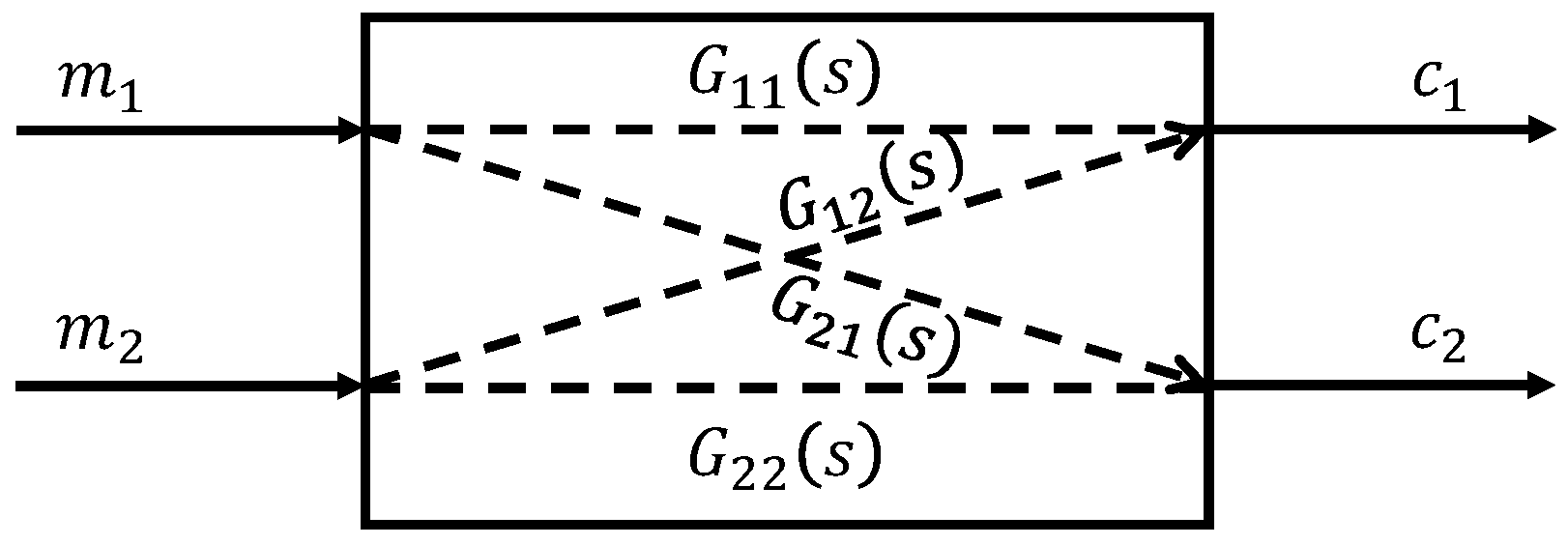
3.1. System Inputs and Outputs

The system inputs are the jet thrust, m 1 , and the propeller angle, m 2 . The system outputs are the USV speed, c 1 , and the USV heading, c 2 . Table 3 also shows the ranges of variation of these variables. The propeller thrust is determined by a pulse-width modulation signal, which enables the engine driver to regulate the power output. The propeller angle is set by a servomotor, which adjusts the nozzle position at the thruster outlet, allowing for the precise direction of the propeller stream. The speed and heading of the USV are determined by GPS and inertial measurement unit (IMU) measurements. These measurements are delivered digitally at a frequency of 10 Hz.
Therefore, it is possible to build a model composed of four transfer functions G i j ( s ) , relating the ith controlled variable with the jth manipulated variable, as shown in Figure 2. G 11 ( s ) and G 12 ( s ) represent the effects of propeller thrust and propeller angle, respectively, on USV speed, while G 21 ( s ) and G 22 ( s ) represent the effects of propeller thrust and propeller angle, respectively, on USV Heading.

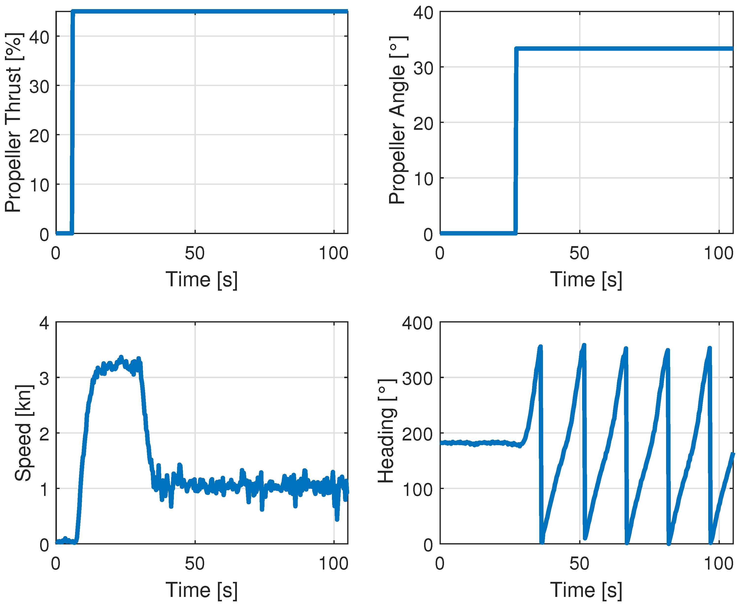
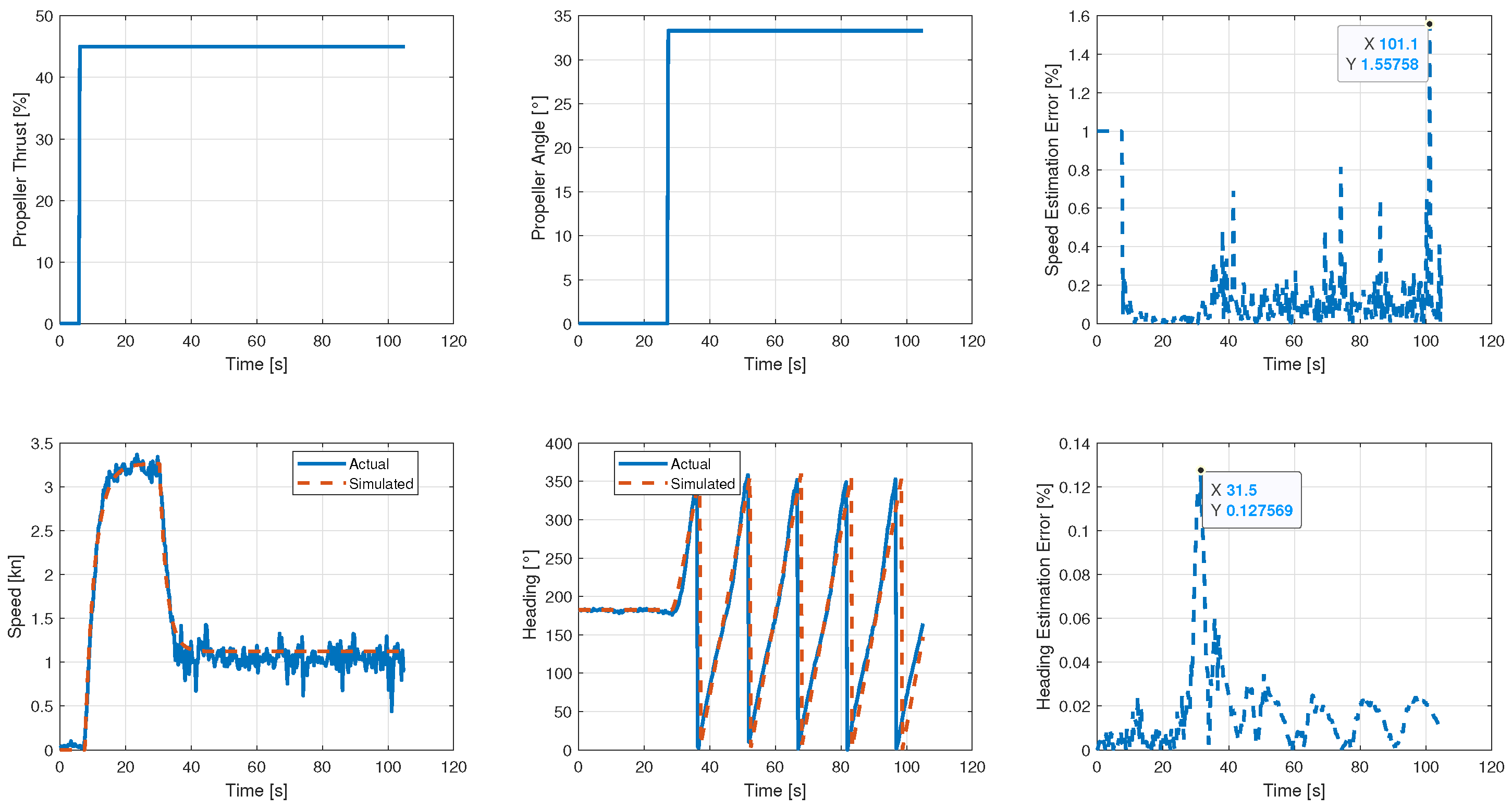
3.2. Experimental Data Generation

Generating the data needed to build the vessel model consists of two stages. First, a constant thrust force is applied through the propeller ( m 1 ) and a steady speed is reached; Figure 1b. Once the USV speed has stabilized, a yaw torque is applied by changing the propeller angle ( m 2 ), making the vessel spin in circles, Figure 1c. It is worth mentioning that the tests were carried out in a 25 m × 50 m pool. Figure 3 shows the vessel’s behavior in the described maneuver.

3.3. USV Proposed Models

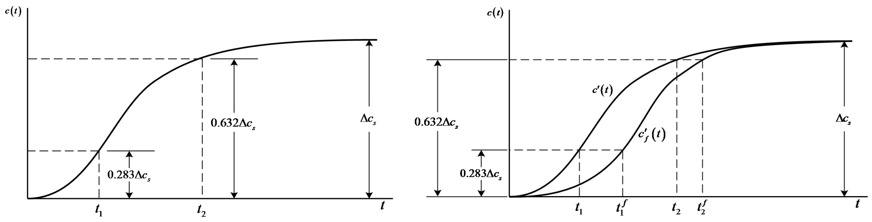
3.3.1. Transfer Function Model

Note that transfer function G 21 ( s ) = 0 indicates that m 1 does not affect c 2 . The above can be seen in Figure 3, where it can be observed that the step change in m 1 does not cause any effect on c 2 . It is only until a change is induced in m 2 that c 2 begins to change. The effects of m 1 and m 2 on c 1 , G 11 ( s ) and G 12 ( s ) , respectively, can be approximated by a First Order Plus Dead Time (FOPDT) model such as that in (1), where K, τ , and t 0 are the process’ gain, constant time, and dead time, respectively.
G ( s ) = K e t 0 s τ s + 1
The model in (1) is an important transfer function used to approximate the response of higher-order processes. The so-called Fit3 method presented in [26] (see Figure 4(Left)) can be used to calculate the parameters of a FOPDT model from the step response of the process as follows.
K = Δ c s Δ m , τ = 1.5 ( t 2 t 1 ) , t 0 = t 2 τ
On the other hand, note the integrating behavior of c 2 —in this case, an Integrating First Order Plus Dead Time (IFOPDT) model (see (3))—can be used to approximate the effects of m 2 on c 2 , that is G 22 ( s ) .
G ( s ) = K e t 0 s s ( τ s + 1 )
The methodology proposed in [27] (see Figure 4(Right)) can be used for the characterization of the integrating processes by solving the equation system composed of (2) and (4) (given t 1 f , t 2 f and τ f = 1.5 ( t 2 f t 1 f ) ).
e ( t 1 t 0 ) τ = τ e ( t 1 f t 0 ) τ τ τ f + τ f e ( t 1 f t 0 ) τ f τ τ f e ( t 2 t 0 ) τ = τ e ( t 2 f t 0 ) τ τ τ f + τ f e ( t 2 f t 0 ) τ f τ τ f
The transfer function matrix model obtained is shown in (5).
c 1 c 2 = G 11 ( s ) G 12 ( s ) G 21 ( s ) G 22 ( s ) m 1 m 2 = K 11 e t 0 11 s τ 11 s + 1 K 12 e t 0 12 s τ 12 s + 1 K 21 e t 0 21 s τ 21 s + 1 K 22 e t 0 22 s s ( τ 22 s + 1 ) m 1 m 2 = 0.07254 e 1.5 s 3 s + 1 0.06431 e 3 s 2.16 s + 1 0 0.7 e s s ( s + 1 ) m 1 m 2
Figure 5 compares the actual and the model responses. The R 2 statistic obtained was 0.9778 and 0.9992 for c 1 and c 2 , respectively. The transfer function matrix model approximates the dynamic response of the actual system quite well, with maximum estimation errors of 1.56 % and 0.13 % for speed and heading, respectively.

3.3.2. State Space Model

The state of a dynamical system is the smallest set of variables (called state variables) such that knowledge of these variables at t = t 0 , together with knowledge of the input to t t 0 , completely determines the system’s behavior at any t t 0 . State-space models use state variables to describe a system using a set of first-order differential Equations (6),
x ˙ ( t ) = A x ( t ) + B u ( t ) y ( t ) = C x ( t )
where x ( t ) is the state vector, u ( t ) is the input vector, y ( t ) is the output vector, A is the state matrix, B is the input matrix, and C is the output matrix.
A state-space model was obtained for the USV using the N4SID algorithm (Numerical Subspace State Space System Identification). The N4SID algorithm is used to identify state-space models of dynamic systems from input–output data [28]. Some of the advantages of this algorithm are the following [29]:
  • No iterative optimization: N4SID is non-iterative and therefore fast.
  • Numerically robust: Uses Singular Value Decomposition, which is stable and reliable.
  • Works well with noise: Especially with short or noisy data records.
The steps followed in N4SID are explained in [30]. Below is a summary of them.
  • Step 1: Construct block Hankel matrices. For a chosen block size i, construct the block Hankel matrices from the data as follows:
    U p = u 1 u 2 u j u 2 u 3 u j + 1 u i u i + 1 u j + i 1 , Y p = y 1 y 2 y j y 2 y 3 y j + 1 y i y i + 1 y j + i 1
    Define the future input–output Hankel matrices U f , Y f . The number of columns j = N 2 i + 1 .
  • Step 2: Toeplitz matrix. Compute the oblique projection of future outputs Y f onto the row space of past data [ U p ; Y p ] , orthogonal to the space covered by U f , as follows:
    P = Proj [ U p ; Y p ] U f ( Y f )
  • Step 3: Singular Value Decomposition (SVD). Apply SVD to the projection matrix:
    P = U Σ V
    The system order n is determined by inspecting the singular values in Σ . Retain the dominant n components as follows:
    Σ 1 = diag ( σ 1 , , σ n ) , U 1 = U ( : , 1 : n )
    Then, estimate the extended observability matrix:
    O i U 1 Σ 1 1 / 2
  • Step 4: Estimate the state sequence. Estimate the state sequence from the following:
    X ^ f = Σ 1 1 / 2 V 1
    where V 1 = V ( : , 1 : n ) .
  • Step 5: Estimate the system matrices. With X ^ k estimated, solve the following equations via least squares:
    X ^ k + 1 = A X ^ k + B u k y k = C X ^ k + D u k
    This yields the state-space matrices A , B , C , and D.
In the USV Sabalo case, the obtained state-space model was x ( t ) = x 1 ( t ) x 2 ( t ) T , u ( t ) = m 1 ( t ) m 2 ( t ) T , y ( t ) = c 1 ( t ) c 2 ( t ) T , and
A = 1.2426 × 10 3 3.3967 × 10 3 1.0803 × 10 1 2.1629 × 10 1 B = 1.7388 × 10 5 6.7773 × 10 5 1.3788 × 10 3 1.3431 × 10 3 C = 4.0251 11.3239 8540.2908 4.7127 .
Therefore, we have two state variables ( n = 2 ), two input variables ( q = 2 ), and two output variables ( p = 2 ). Note that the state variables x 1 ( t ) and x 2 ( t ) are abstract; therefore, they cannot be quantified directly. Figure 6 compares the actual and the state space model responses. The statistic R 2 obtained was 0.9271 and 0.9985 for c 1 and c 2 , respectively. The state-space model approximates the dynamic response of the actual system quite well, with maximum estimation errors of 18.7 % and 0.3 % for speed and heading, respectively.

4. Unmanned Surface Vehicle Control

Two control strategies were implemented for the vessel as follows: one based on two independent control loops with decoupler blocks, and the other on state variable feedback with a state estimator. Both alternatives are presented below.

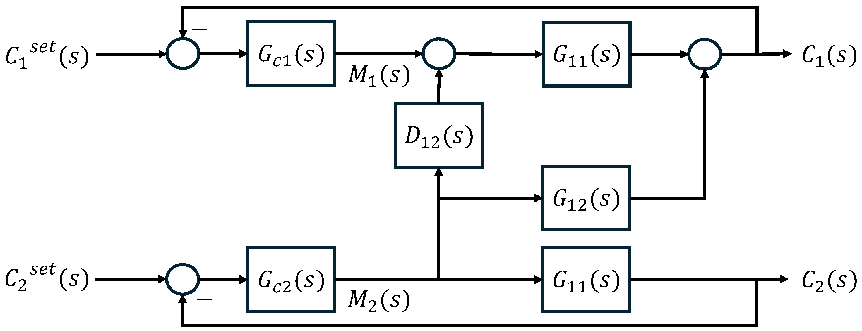
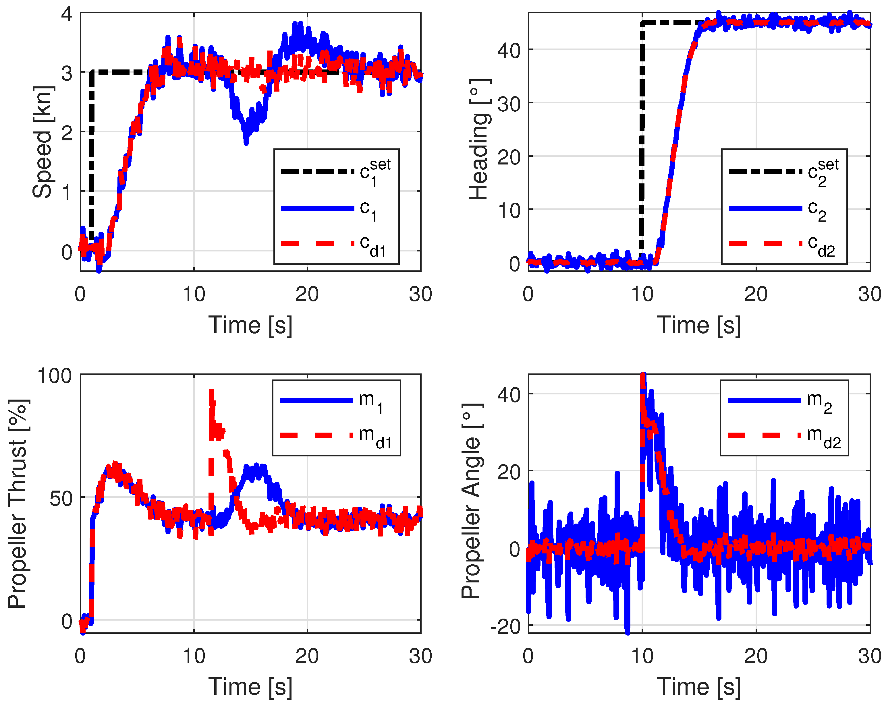
4.1. Control Strategy 1—Independent Control Loops with Decoupling of Interactions

Figure 7 presents the block diagram for the proposed strategy. The decoupled block D 12 ( s ) is installed to cancel the effect of m 2 on c 1 .
G c 1 ( s ) is PI controller tuned with the lambda tuning method [31], while G c 2 ( s ) is a PD controller tuned with the approach proposed in [27] for the integrating process. The parameters of each controller are presented in Table 4.
On the other hand, from the block diagram algebra, we can derive
C 1 ( s ) M 2 ( s ) = G 11 ( s ) D 12 ( s ) + G 12 ( s ) = 0 .
By solving the decoupler transfer function from (15) and replacing G 11 ( s ) and G 12 ( s ) from (5), we obtain
D 12 ( s ) = G 12 ( s ) G 11 ( s ) = ( 1.231 s + 0.4104 ) ( s + 0.463 ) e 1.5 s
The experimental tests were conducted in a controlled environment, as follows: a pool with calm water, a surface free from obstacles, and with the vessel floating horizontally. Setpoints for speed and heading were selected so the vessel remained well away from the pool’s edges to protect it from potential collisions. Figure 8 shows the response of control systems without a decoupler ( c 1 and c 2 ) and with decoupler ( c d 1 and c d 2 ). The systems are excited with an increase of 3 kn in c 1 s e t and a subsequent 45° increase in the c 2 s e t , the setpoints for speed and heading, respectively.
In the case of the control system without a decoupler (blue continuous line), the interaction effect is observed in c 1 once the change in c 2 s e t is generated, that is, the oscillation in the speed at t = 10 s. However, when the decoupler is included (red dashed line), it is observed that the interaction effect is wholly canceled, c d 1 . It is essential to highlight that the limits of the manipulated variables are not exceeded.

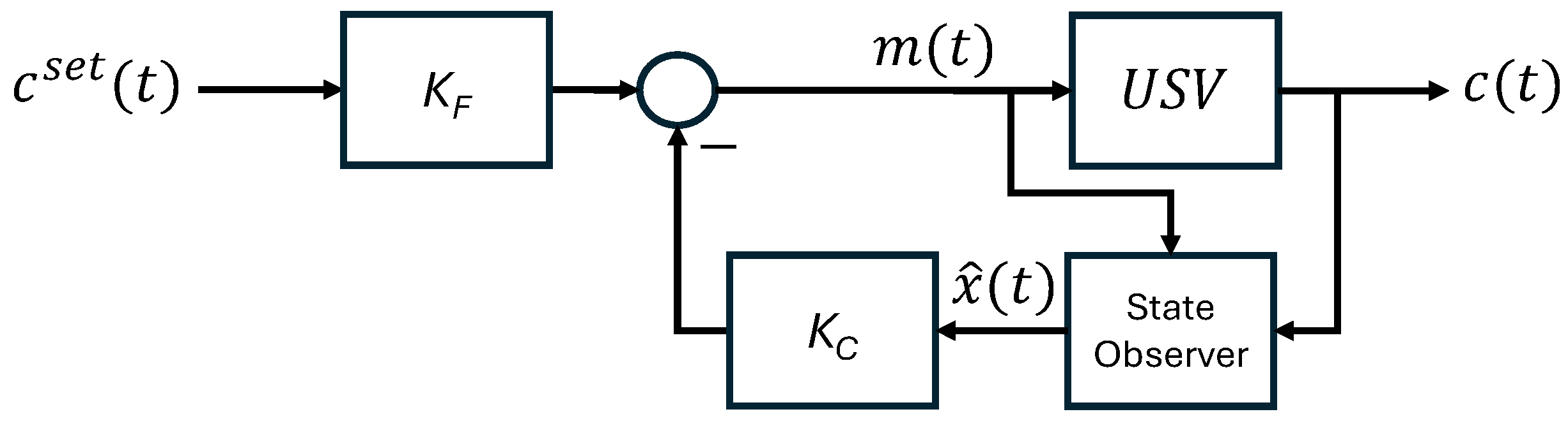
4.2. Control Strategy 2—State Feedback Control

In this case, the state-space realization in (6) was used to develop a control strategy based on state feedback, as shown in Figure 9. The state feedback gain, K C , was calculated as follows:
  • Step 1. Check controllability: Construct the controllability matrix.
    C = B A B A 2 B A n 1 B
    If rank ( C ) = n , the system is controllable, and you may proceed. Otherwise, full pole placement is not possible.
  • Step 2. Calculate the characteristic polynomial of A.
    Δ ( s ) = det ( s I A ) = s n + α n 1 s n 1 + + α 1 s + α 0
  • Step 3. Choose the desired closed-loop poles: Select n desired eigenvalues { λ 1 , λ 2 , , λ n } based on the desired transient response and stability. Compute the desired characteristic polynomial.
    Δ des ( s ) = ( s λ 1 ) ( s λ 2 ) ( s λ n ) Δ des ( s ) = s n + α ¯ n 1 s n 1 + + α ¯ 1 s + α ¯ 0
  • Step 4. Calculate the feedback gains for the equivalent controllable canonical form.
    K ¯ C = α ¯ n 1 α n 1 α ¯ 1 α 1 α ¯ 0 α 0
  • Step 5. Calculate the equivalence transformation.
    S : = P 1 = B A B A 2 B A n 1 B 1 α n 1 α 1 α 0 0 1 α n 1 α 1 0 0 0 1 α n 1 0 0 0 0 1
  • Step 6. Calculate feedback gains K C = K ¯ C P = K ¯ C S 1 .
Since the state variables in the state-space model in (14) are abstract and cannot be directly quantified, it was necessary to integrate a state observer into the control strategy, as shown in Figure 9. The output x ^ ( t ) of the observer is governed by (22). Calculating the estimator gain, L, by transposing matrix A and replacing C T with matrix B in the above procedure to calculate K C is possible.
x ^ ˙ ( t ) = ( A L C ) x ^ ( t ) + B m ( t ) + L c ( t )
The state feedback control strategy in Figure 9 includes a pre-filter gain K F to guarantee that the controlled variable is commanded to track a setpoint asymptotically (setpoint tracking).
Let c s e t denote a desired constant value for the output c ( t ) . The control objective is to design a control law, which may depend on x ( t ) and c s e t , so that the closed-loop control system is stable and that the tracking error e ( t ) = c s e t c ( t ) tends to zero as t . Since c s e t 0 , the steady-state value of x ( t ) , x s s cannot be 0. Assume that a control law has been chosen so that both x ( t ) and m ( t ) converge to a steady-state value as t . Therefore, in a steady state, (6) can be written in matrix form as in (23).
A B C 0 x s s m s s = 0 I q c s e t
where 0 is a zero matrix of size n × q , x s s = lim t x ( t ) and m s s = lim t m ( t ) are steady-state values of the state and manipulated variables, respectively, with I q being a q × q identity matrix.
If A B C 0 is nonsingular, (23) can be solved uniquely for x s s m s s T , as in (24).
x s s m s s = A B C 0 1 0 I q c s e t
Furthermore, by considering the state feedback control law m = m s s K C ( x x s s ) , which can be rewritten as follows
m = m s s K C ( x x s s ) = K C I p x s s m s s K C x = K C I q A B C 0 1 0 I q c s e t K C x = K F c s e t K C x
we obtain that
K F = K C I q A B C 0 1 0 I q .
It is worth mentioning that the previous result guarantees setpoint tracking for constant step reference inputs. For high-order reference inputs, integral actions must be included in the control strategy [32]. Equation (26) was used to calculated the K C in (27).
The gains of the state feedback K C , state observer L, and pre-filter K F are shown in (27). Closed-loop poles were chosen at 0.8 and 0.9 , and observer poles were chosen five times faster than closed-loop poles.
K C = 2.8823 × 10 4 241.6017 2.9511 × 10 4 112.1038 L = 9.0898 × 10 4 1.5 × 10 3 0.2899 1.4929 × 10 4 K F = 34.4597 3.3822 10.6382 3.4507
Experimental tests were conducted under the same conditions described above. Figure 10 shows the response of the state feedback control, where c 1 S F B and c 2 S F B are the controlled variables obtained with the state feedback control strategy. The system was excited with an increase of 3 kn in c 1 s e t and a subsequent increase of 45° in c 2 s e t , as in the previous case.
The Integral Absolute Error (IAE) index, I I A E = 0 t f | e ( t ) | d t , was used to evaluate the performance of the control strategies. The IAE serves as a performance metric in control systems, quantifying the cumulative magnitude of tracking errors over time without regard to their sign. Lower IAE values signify improved tracking accuracy. This metric is commonly used in controller optimization to ensure a smoother system response, minimizing control effort. Table 5 shows the results obtained. Regarding control strategy 1, with control strategy 2, 35.89% and 72.31% reductions are obtained in the IAE indices for speed and heading, respectively.

5. Discussion

Transfer function matrix and state-space models were used to model the vessel. In both cases, the models’ responses, Figure 5 and Figure 6, are very close to the behavior of the actual system. Although the literature contains a wide range of complex models and parameter identification techniques applicable to USVs [8,15,33,34], whose results show satisfactory consistency between the predictions of the proposed models and the test data, the models proposed here show similar results in terms of estimation errors but stand out for their simplicity. The high value of the speed estimation error observed initially in the state-space model, 18.7 % , is because the model induces an apparent effect of m 1 on c 2 ; however, estimation errors below 1.65 % are observed from that point onward. This initial peak estimation error does not occur in the model based on the transfer function because G 21 ( s ) = 0 is set.
Some advantages associated with the simplicity of the models used are as follows:
  • Interpretability: Simple models are often more transparent and intuitive, making understanding the system’s behavior easier.
  • Efficiency: Simpler models typically require fewer computations, making them ideal for real-time applications or iterative simulations.
  • Lower hardware demands.
  • Reduced data requirements: With fewer parameters, you need less experimental or observational data to calibrate the model.
  • Lower risk of overfitting: Simple models are more robust, especially in noisy or limited datasets.
  • Control-friendly: Many classic control strategies assume linear or low-order models.
  • Observability and controllability: These properties are more straightforward to verify and maintain in simple systems.
  • Closed-form solutions: Simpler models often allow for analytical solutions or approximations, revealing key insights into the dynamics.
  • Sensitivity analysis: Easier to assess how parameters influence outcomes.
  • Model verification: Simpler structures facilitate the identification of errors or inconsistencies in the model assumptions.
  • Baseline comparison: Simple models provide a reference for testing the added value of complexity.
  • Iterative improvement: Based on performance gaps, you can progressively add complexity as needed.
Regarding the performance of the control strategies, we can again state that simple control techniques show promising results. Figure 8 shows the benefits of including the decoupler block, achieving the complete elimination of the effect of the angle of the propeller ( m 2 ) on the vessel’s speed ( c 1 ). Generally, this strategy shows good response times without exceeding the limits of the manipulated variables (actuator saturation). Figure 10 allows us to compare the performance of both control strategies. In this case, better response times are observed with the state feedback strategy, reflected in the better performance indices (Table 5). However, as expected, the shorter response times imply greater energy consumption, reflected in the higher values in the manipulated variables. Additionally, the small effect of the propeller’s thrust ( m 1 ) on the vessel’s heading ( c 2 ) is observed, which does not occur in the previous strategy. However, the response speeds achieved make this strategy attractive for combat maneuvers.
Some advantages of classical control techniques, such as those used in this work, are as follows:
  • Simple structure and intuitive understanding: Easy to implement with minimal code or analog components. Tuning can be performed using basic heuristics or a trial-and-error approach. Little specialist knowledge is needed; it is widely taught and used.
  • Required system knowledge and modeling: It can often work with no explicit or straightforward model (e.g., gain and time constant). Design focuses on measured behavior (e.g., step response and frequency response).
  • Very low computational load: It can run on inexpensive hardware or analog circuits. It is suitable for high sampling rates and fast dynamics.
  • Real-world applicability: It is ideal for single-variable or loosely coupled systems, and these approaches are widely used in typical engineering applications due to their quick deployment and well-understood nature.

6. Conclusions

This work presents an unmanned surface vehicle’s modeling and control design, focusing on dynamic characterization and the evaluation of control strategies. Two modeling approaches, transfer function and state-space representations, were developed using experimental data collected under controlled test conditions. The resulting models closely approximate the system’s behavior with high statistical accuracy ( R 2 > 0.9 ), validating their suitability for control design. Note that, although the model fit was excellent for the tested scenario, as evidenced by the high correlation coefficients presented, this level of accuracy cannot be guaranteed under different operating conditions, such as significant variations in propeller thrust or angle, without further validation or model recalibration. Accordingly, the reported correlation coefficients should not be interpreted as a universal indicator of model accuracy. Instead, they reflect the fit quality within the specific context and conditions under which the experimental data were collected and the models were derived.
While the literature presents a wide range of complex modeling and identification techniques for USVs, which also yield good agreement between predicted and measured dynamics, the models proposed here are distinguished by their simplicity. Despite this, they offer comparable performance in terms of estimation error. In the state-space model, an initial peak estimation error is observed due to an apparent induced interaction between propeller thrust and heading; however, subsequent errors remain consistently low. This effect is absent in the transfer function model.
Building on these models, two classical control strategies were designed and analyzed. Independent loop control with a decoupling block successfully eliminates the effect of propeller angle on the vessel speed. This strategy offers acceptable response times while keeping manipulated variables within operational limits, making it suitable for long-duration and energy-conscious missions such as humanitarian or environmental operations. On the other hand, we have a state feedback control, which provides faster dynamic responses, particularly advantageous for applications requiring agility and rapid maneuvering (e.g., tactical or evasive actions). The results confirm the improved performance indices compared to the first strategy. However, this performance comes at the cost of increased control effort, reflected in the higher actuator usage and energy consumption.
The successful application of classical control techniques further underscores their continued relevance and effectiveness in modern autonomous systems. Some of their key benefits include the following: ease of implementation and tuning with minimal computational resources, compatibility with simple models or empirical data, and low-cost deployment on embedded systems or resource-constrained platforms.
Experimental validation in real-world marine environments can only fully assess the robustness of the proposed models and control strategies. These tests, planned as part of future work, will provide a more comprehensive evaluation of the models’ predictive capabilities and control systems’ performance under the influence of environmental disturbances and varying operating regimes. This will also offer valuable insights into the potential refinements needed for deployment in operational scenarios.

Author Contributions

Conceptualization, A.L.-A. and C.A.G.-M.; methodology, project administration and validation, J.F.J.-V. and J.E.-G.; experimentation, mathematical analysis, simulations, writing—original draft preparation, and writing—review and editing, J.J.-C. and R.S.-D. The authors contributed equally to this work. All authors have read and agreed to the published version of the manuscript.

Funding

This work was possible thanks to funding from the Ministry of Science, Technology and Innovation of Colombia (Minciencias), under the framework collaboration agreement N° 1038-2022 to develop the project “River Vessel Surveillance and Monitoring System”. We also thank the Escuela Naval de Cadetes “Almirante Padilla” (ENAP) and Escuela de Formación de Infantería de Marína (EFIM) for their valuable assistance in carrying out the online surveys that contributed to the development of this research.

Data Availability Statement

The data presented in this study are available on request from the corresponding author due to privacy restrictions.

Conflicts of Interest

The authors declare no conflicts of interest.

Abbreviations

The following abbreviations are used in this manuscript:
FOPDTFirst Order Plus Dead Time
GPSGlobal Position System
IAEIntegral Absolute Error
IFOPDTIntegral First Order Plus Dead Time
IMUInertial Measurement Unit
PIProportional-Integral
PDProportional-Derivative
PIDProportional-Integral-Derivative
SMCSliding Mode Control
USVUnmanned Surface Vehicles
PWMPulse Width Modulation
NMEANational Marine Electronics Association

References

  1. Qiao, Y.; Yin, J.; Wang, W.; Duarte, F.; Yang, J.; Ratti, C. Survey of deep learning for autonomous surface vehicles in marine environments. IEEE Trans. Intell. Transp. Syst. 2023, 24, 3678–3701. [Google Scholar] [CrossRef]
  2. Sanjou, M.; Shigeta, A.; Kato, K.; Aizawa, W. Portable unmanned surface vehicle that automatically measures flow velocity and direction in rivers. Flow Meas. Instrum. 2021, 80, 101964. [Google Scholar] [CrossRef]
  3. Katsouras, G.; Dimitriou, E.; Karavoltsos, S.; Samios, S.; Sakellari, A.; Mentzafou, A.; Tsalas, N.; Scoullos, M. Use of Unmanned Surface Vehicles (USVs) in Water Chemistry Studies. Sensors 2024, 24, 2809. [Google Scholar] [CrossRef]
  4. Mancini, A.; Frontoni, E.; Zingaretti, P.; Longhi, S. High-resolution mapping of river and estuary areas by using unmanned aerial and surface platforms. In Proceedings of the 2015 International Conference on Unmanned Aircraft Systems (ICUAS), Denver, CO, USA, 9–12 June 2015; IEEE: New York, NY, USA, 2015; pp. 534–542. [Google Scholar]
  5. Jorge, A.; Vitorino, J.; Fonseca, J. Unmanned Surface Vehicles in the Maritime Environment: A Review. Sensors 2019, 19, 702. [Google Scholar] [CrossRef]
  6. Abrougui, H.; Nejim, S.; Hachicha, S.; Zaoui, C.; Dallagi, H. Modeling, parameter identification, guidance and control of an unmanned surface vehicle with experimental results. Ocean Eng. 2021, 241, 110038. [Google Scholar] [CrossRef]
  7. Setiawan, F.A.; Kadir, R.E.A.; Gamayanti, N.; Santoso, A.; Bilfaqih, Y.; Hidayat, Z. Dynamic modelling and controlling Unmanned Surface Vehicle. IOP Conf. Ser. Earth Environ. Sci. 2021, 649, 012056. [Google Scholar] [CrossRef]
  8. Zhang, Z.; Ren, J. Non-parametric dynamics modeling for unmanned surface vehicle using spectral metric multi-output Gaussian processes learning. Ocean Eng. 2024, 292, 116491. [Google Scholar] [CrossRef]
  9. Xu, P.F.; Cheng, C.; Cheng, H.X.; Shen, Y.L.; Ding, Y.X. Identification-based 3 DOF model of unmanned surface vehicle using support vector machines enhanced by cuckoo search algorithm. Ocean Eng. 2020, 197, 106898. [Google Scholar] [CrossRef]
  10. Zhong, Y.; Yu, C.; Cao, J.; Liu, C.; Lian, L. Modeling and Control of Unmanned Surface Vehicles: An Integrated Approach. In Proceedings of the 8th International Conference on Automation, Control and Robotics Engineering (CACRE), Hong Kong, China, 13–15 July 2023; pp. 979–984. [Google Scholar] [CrossRef]
  11. Ma, Y.; Liu, Z.; Wang, T.; Song, S.; Xiang, J.; Zhang, X. Multi-model predictive control strategy for path-following of unmanned surface vehicles in wide-range speed variations. Ocean Eng. 2024, 295, 116845. [Google Scholar] [CrossRef]
  12. Wang, X.; Yi, H.; Xu, J.; Xu, C.; Song, L. PID Controller Based on Improved DDPG for Trajectory Tracking Control of USV. J. Mar. Sci. Eng. 2024, 12, 1771. [Google Scholar] [CrossRef]
  13. Zhou, Y.; Gong, C.; Chen, K. Adaptive Control Scheme for USV Trajectory-Tracking under Complex Environmental Disturbances via Deep Reinforcement Learning. IEEE Internet Things J. 2025, early access. [Google Scholar] [CrossRef]
  14. Cheng, M.; Yao, J.; Ren, Q. A Model Predictive Control Approach for USV Autonomous Cruising via Disturbance Learning. In Proceedings of the 2024 IEEE 18th International Conference on Control & Automation (ICCA), Reykjavík, Iceland, 18–21 June 2024; IEEE: New York, NY, USA, 2024; pp. 988–993. [Google Scholar]
  15. Ding, K.; Zhu, Q. Network-Based Modeling and Sampling Guaranteed Cost Control for Unmanned Surface Vehicle Systems Under Stochastic Cyber-Attacks. IEEE Trans. Intell. Transp. Syst. 2024, 25, 6173–6185. [Google Scholar] [CrossRef]
  16. Xue, S.; Zhao, N.; Zhang, W.; Luo, B.; Liu, D. A Hybrid Adaptive Dynamic Programming for Optimal Tracking Control of USVs. IEEE/ASME Trans. Mechatronics 2024, early access. [Google Scholar] [CrossRef]
  17. Yancai, H.; Yang, L.; Yan, Z.; Hoang, D.T.M. Adaptive Formation Control for Obstacle Avoidance of USVs with Asymmetric Input Saturation. Sci. Rep. 2024, 14, 73560. [Google Scholar] [CrossRef]
  18. Martínez-León, A.S.; Jatsun, S.; Emelyanova, O. Investigation of Wind Effects on UAV Adaptive PID Based MPC Control System. Enfoque UTE 2024, 15, 36–47. [Google Scholar] [CrossRef]
  19. Mahesh, K.; Sharma, A.; Peters, A.; Mehra, R.; Pascoal, A.; Williams, B. Safe Autonomy for Uncrewed Surface Vehicles Using Adaptive Control and Reachability Analysis. arXiv 2024, arXiv:2410.01038. [Google Scholar] [CrossRef]
  20. Castano-Londono, L.; Marrugo Llorente, S.d.P.; Paipa-Sanabria, E.; Orozco-Lopez, M.B.; Fuentes Montaña, D.I.; Gonzalez Montoya, D. Evolution of Algorithms and Applications for Unmanned Surface Vehicles in the Context of Small Craft: A Systematic Review. Appl. Sci. 2024, 14, 9693. [Google Scholar] [CrossRef]
  21. Thomas, A.R.; PS, L.P.; Kumar, H. Disturbance Estimation and Rejection in an Underwater Autonomous Vehicle. In Proceedings of the 2024 International Conference on E-mobility, Power Control and Smart Systems (ICEMPS), Thiruvananthapuram, India, 18–20 April 2024; IEEE: New York, NY, USA, 2024; pp. 1–6. [Google Scholar]
  22. Barrera, C.; Maarouf, M.; Campuzano, F.; Llinas, O.; Marichal, G.N. A Comparison of Intelligent Models for Collision Avoidance Path Planning on Environmentally Propelled Unmanned Surface Vehicles. J. Mar. Sci. Eng. 2023, 11, 692. [Google Scholar] [CrossRef]
  23. Wu, X.; Wei, C. DRL-Based Motion Control for Unmanned Surface Vehicles with Environmental Disturbances. In Proceedings of the 2023 IEEE International Conference on Unmanned Systems (ICUS), Hefei, China, 13–15 October 2023; IEEE: New York, NY, USA, 2023; pp. 1696–1700. [Google Scholar]
  24. Yue, X. UsV Course Control strategy based on the Disturbance Observer Under Disturbances of winds and waves. In Proceedings of the 2023 Smart City Challenges & Outcomes for Urban Transformation (SCOUT), Singapore, 29–30 July 2023; IEEE: New York, NY, USA, 2023; pp. 76–80. [Google Scholar]
  25. Miao, R.; Dong, Z.; Wan, L.; Zeng, J. Heading control system design for a micro-USV based on an adaptive expert S-PID algorithm. Pol. Marit. Res. 2018, 25, 6–13. [Google Scholar] [CrossRef]
  26. Smith, C.A.; Corripio, A.B. Principles and Practices of Automatic Process Control; John Wiley & Sons: Hoboken, NJ, USA, 2005. [Google Scholar]
  27. Jorge, C.C.; Jorge, H.N.; Wendell, M.R.; Edalatpanah, S.; Shariq, A.B.; Naz, S.; Javier, J.C.; Gabriel, P.E. Novel characterization and tuning methods for integrating processes. Int. J. Inf. Technol. 2024, 16, 1387–1395. [Google Scholar] [CrossRef]
  28. Van Overschee, P.; De Moor, B. Subspace Identification for Linear Systems: Theory—Implementation—Applications; Springer Science & Business Media: Cham, Switzerland, 2012. [Google Scholar]
  29. Zeno, A.; Omtveit, M.; Uhlen, K. Improvement of System Identification using N4SID and DBSCAN Clustering for Monitoring of Electromechanical Oscillations. In Proceedings of the 2023 IEEE Belgrade PowerTech, Belgrade, Serbia, 25–29 June 2023; IEEE: New York, NY, USA, 2023; pp. 1–6. [Google Scholar]
  30. Ma, H.; Yang, D.; Qin, H.; Cao, Y.; Cheng, D.; Zhang, B.; Hao, X.; Zhou, N. Power System Equivalent Inertia Estimation Method Using System Identification. In Proceedings of the 2022 IEEE 5th International Conference on Electronics Technology (ICET), Chengdu, China, 13–16 May 2022; IEEE: New York, NY, USA, 2022; pp. 360–365. [Google Scholar]
  31. Coughran, M.T. Lambda Tuning—the Universal Method for PID Controllers in Process Control. Control. Glob. Digit. Ed. 2013. Available online: https://www.controlglobal.com/articles/2013/lambda-tuning-universal-method-for-pid-controllers/ (accessed on 1 March 2025).
  32. Huang, B.; Lu, B.; Li, Q. A proportional–integral-based robust state-feedback control method for linear parameter-varying systems and its application to aircraft. Proc. Inst. Mech. Eng. Part G J. Aerosp. Eng. 2019, 233, 4663–4675. [Google Scholar] [CrossRef]
  33. Zhang, M.; Li, D.; Xiong, J.; He, Y. GBM-ILM: Grey-Box Modeling Based on Incremental Learning and Mechanism for Unmanned Surface Vehicles. J. Mar. Sci. Eng. 2024, 12, 627. [Google Scholar] [CrossRef]
  34. Xu, F.; Zhang, K.; Song, S.; Xie, Y. Simulation Technology of Unmanned Surface Vehicle Cluster Based on Digital Modeling. In Proceedings of the International Conference on Autonomous Unmanned Systems, Nanjing, China, 9–11 September 2023; Springer: Singapore, 2023; pp. 37–48. [Google Scholar]
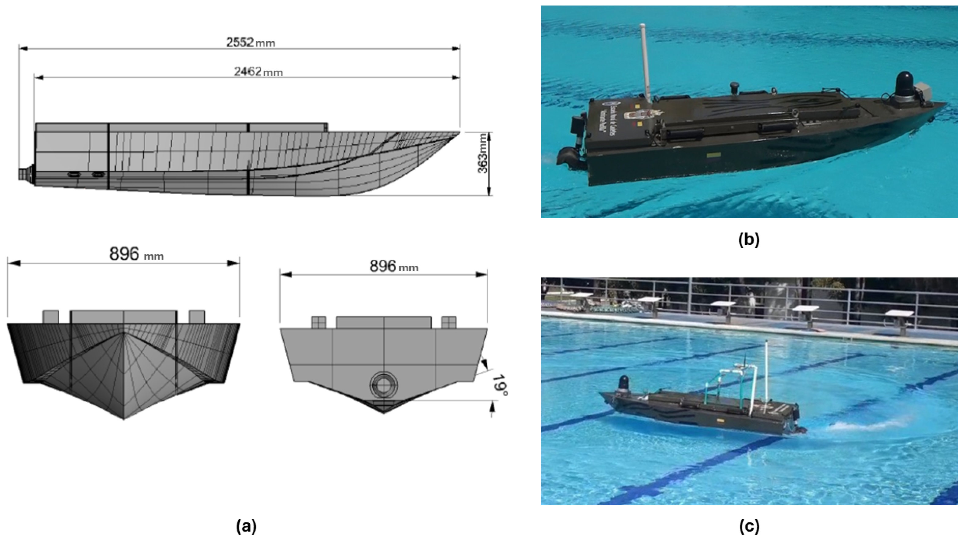
Figure 1. Prototype USV SABALO: (a) USV dimensions, (b) USV linear motion, and (c) USV spin in circle.
Jmse 13 00813 g001
Figure 2. Step response of the unmanned surface vehicle.
Jmse 13 00813 g002
Figure 3. Step response of the unmanned surface vehicle.
Jmse 13 00813 g003
Figure 4. Characterization methods. (Left) Fit3. (Right) Filtered Fit3.
Jmse 13 00813 g004
Figure 5. Transfer matrix model step response.
Jmse 13 00813 g005
Figure 6. State-space model step response.
Jmse 13 00813 g006
Figure 7. Independent control loops with a decoupler.
Jmse 13 00813 g007
Figure 8. Response of independent control loops with a decoupler.
Jmse 13 00813 g008
Figure 9. State feedback control.
Jmse 13 00813 g009
Figure 10. State feedback control loop response.
Jmse 13 00813 g010
Table 2. USV parameters.
ParameterValue
Length2462 mm
Beam896 mm
Draft15 mm
Weight117 kg
Speed9 kn
Table 3. System inputs and outputs variables.
TypeVariableSymbolRange
InputPropeller Thrust m 1 0∼100 %
Propeller Angle m 2 −45°∼45°
OutputUSV Speed c 1 0∼9 kn
USV Heading c 2 0°∼360°
Table 4. PI and PD controller parameters.
ControllerParameterValue
PI K c 1 = τ 11 2 K 11 t 0 11 13.7861
τ i 1 = τ 11 3
PD K c 2 = τ 22 2 K 22 t 0 22 0.7143
τ d 2 = τ 22 1
Table 5. Performance indices.
Control StrategyIAE Index
1 IAE c 1 = 12.39
IAE c 2 = 136.9
2 IAE c 1 = 7.943
IAE c 2 = 37.91
Disclaimer/Publisher’s Note: The statements, opinions and data contained in all publications are solely those of the individual author(s) and contributor(s) and not of MDPI and/or the editor(s). MDPI and/or the editor(s) disclaim responsibility for any injury to people or property resulting from any ideas, methods, instructions or products referred to in the content.

