Abstract
The randomness and complexity of ice loads present major challenges to the safety and stability of offshore platforms. Traditional methods for identifying ice loads often lack accuracy and adaptability under changing environmental conditions. This study proposes a novel inversion method based on Temporal Convolutional Networks (TCNs), integrating finite element simulation with deep learning to effectively identify random ice loads. A random ice load model is first developed, and its dynamic characteristics are validated through finite element analysis. The TCN model is then applied to capture the time-dependent features of ice loads. To improve the model’s generalization ability, its hyperparameters are optimized using particle swarm optimization (PSO). The results show that the TCN model achieves goodness-of-fit (R2) values of 0.821 and 0.808 on the training and test sets, respectively, indicating strong predictive performance. Under different ice thickness and velocity conditions, the model achieves R2 values close to 0.99, demonstrating high robustness. This work represents the first application of TCN to ice load identification. By combining it with simulation data, we offer a high-precision, data-driven approach for dynamic load identification, enhancing the efficiency and reliability of safety assessments for conical offshore platforms.
1. Introduction
The stability of ice-resistant offshore platforms is essential for the safe and reliable operation of marine structures [1]. Among the various environmental loads they face, ice loads are particularly difficult to manage due to their random nature and sensitivity to changing conditions. The mechanical behavior of sea ice is complex and depends on several factors such as temperature, ice thickness, shape, and drift speed [2,3]. Under random ice loading, platforms may experience dynamic effects like resonance and fatigue, which can reduce structural safety over time. Therefore, accurately identifying and evaluating ice loads is a key requirement in the design and maintenance of offshore platforms [4].
Traditional ice load identification methods are mainly based on simplified physical models and empirical equations [5]. These methods typically use measured environmental parameters, such as ice thickness and speed, to estimate the loads using fixed formulas [6,7]. In recent years, the development of sensor technology and data acquisition systems has made real-time monitoring of ice–structure interactions more feasible [8,9]. However, even with more monitoring data, traditional methods still face limitations in accuracy and adaptability, especially under extreme or rapidly changing ice conditions [10].
With the growing use of artificial intelligence and data-driven techniques, there is increasing interest in applying machine learning and deep learning methods to ice load identification [11,12]. These methods can learn complex relationships between structural responses and external loads directly from data, without relying on predefined physical models. This allows for more flexible and accurate modeling across a wider range of ice conditions [13].
Among the available deep learning methods, the Temporal Convolutional Network (TCN) has shown strong potential for analyzing time-series data. TCNs use dilated causal convolutions to capture long-term dependencies in data while avoiding problems like vanishing gradients that affect traditional recurrent models. Residual connections are also used to improve training efficiency and model stability [14].
Compared to other sequence models such as Recurrent Neural Networks (RNNs) and Long Short-Term Memory (LSTM) networks, TCNs are better at preserving time sequence information and can process data more efficiently due to their ability to run in parallel [15,16,17]. These advantages make TCNs well-suited for identifying time-varying ice loads based on structural response data.
In this study, a method is proposed to identify random ice loads on conical offshore platforms using a TCN-based model. The approach combines finite element simulations and real monitoring data to train a model that can accurately reconstruct ice load time histories. The goal is to improve the accuracy, efficiency, and robustness of ice load prediction, contributing to better safety assessment and operational planning for offshore platforms in cold regions.
2. On-Site Monitoring of Platforms
2.1. Overview and Characteristics of Ice-Resistant Platforms
The JZ20-2 NW platform is an ice-resistant offshore structure that was constructed and commissioned in 2005, as shown in Figure 1. The platform features a single-leg jacket structure, designed to operate in a water depth of 13.5 m. The jacket weighs approximately 250 tons, and the topside equipment weighs about 228 tons. The static stiffness at the waterline is 6.10 × 10⁷ N/m.
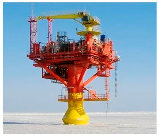
Figure 1.
JZ20-2 NW platform.
The main leg of the platform has a diameter of 3.5 m and is equipped with an ice-breaking cone at the water surface. This cone consists of two sections—an upper and a lower segment—each with an angle of 60 degrees. The maximum diameter of the cone reaches 6 m. The main leg is supported by three skirt piles, each with an underwater diameter of 1.3 m. These piles are connected to the leg by three horizontal braces, providing additional structural stability.
The platform includes two decks—an upper and a lower one. To mitigate ice-induced vibrations, vibration isolation pads and magnetorheological dampers are installed between the two decks. This design not only enhances the platform’s ice-resistance performance but also reduces the amount of structural steel required, optimizing material usage while maintaining safety and functionality.
2.2. On-Site Monitoring of Ice Force Measurement
The JZ20-2 NW platform is a new-generation ice-resistant jacket structure developed to meet the production demands of marginal oil fields in the Bohai Sea. The layout of its on-site monitoring system is shown in Figure 2. The primary objective of the monitoring system is to measure ice-induced vibration responses and collect relevant sea ice parameters.

Figure 2.
Sensor locations of the NW platform.
Ice-induced vibrations are monitored using acceleration sensors installed in the platform’s central control room. These sensors are configured orthogonally to capture acceleration data in two vertical directions, as illustrated in Figure 3. To acquire sea ice parameters, such as ice velocity and thickness, cameras are installed on the lower deck. These cameras are used to continuously record ice–structure interactions, as shown in Figure 4.
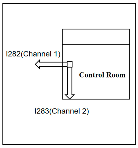
Figure 3.
Layout diagram of accelerometer on JZ20-2 NW upper deck.
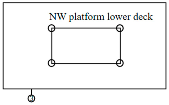
Figure 4.
Layout diagram of the camera on JZ20-2 NW upper deck.
This integrated monitoring system enables the collection of real-time, multi-dimensional data related to both structural responses and environmental ice conditions. Such data are essential for analyzing ice–structure interaction mechanisms and for validating computational models used in ice load prediction and structural response simulation.
2.3. Processing and Organization of Ice Force Data
In this study, ten typical ice–structure interaction events observed on the JZ20-2 NW platform were selected for analysis. Each event represents a distinct working condition with varying ice parameters, including differences in ice thickness, ice velocity, and structural vibration responses. For each case, vibration acceleration data within a 5-minute window surrounding the event were processed and compiled.
Additionally, the maximum daily ice thickness observed during the monitoring period was recorded, along with the corresponding ice velocity and other relevant sea ice parameters.
Key parameters extracted from the field monitoring videos include ice thickness, ice velocity, the length of ice bending failure, and the structural width at the waterline. These measurements were obtained using pixel-based distance analysis in Adobe Photoshop (PS), applied to calibrated video frames.
The data processing procedure consists of the following steps:
- (1)
- Calibration and Scale Conversion
Reference objects—such as rulers, structural members (e.g., pile legs), or wave-dissipating holes—are identified within the video frames. Their known dimensions are used to calculate a pixel-to-length conversion factor by measuring their pixel lengths in the image.
- (2)
- Ice Thickness Measurement
After interaction with the structure, broken ice fragments typically flip before submerging, momentarily exposing their cross-sections. These instances are captured by fixed cameras. By referencing known dimensions in the same frame and maintaining a constant focal length, the ice thickness can be calculated from the image. For example, a measurement line is drawn along the ice section; the pixel width is identified using the transformation panel, and the actual thickness is calculated based on the pixel-to-length ratio. If a 1-meter calibration ruler measures 127.03 pixels, the scale is determined to be 1/127.03 = 0.00787 m/pixel, as illustrated in Figure 5.
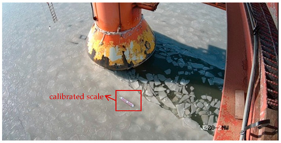
Figure 5.
Determining the unit pixel distance.
This method allows for reliable quantification of varying ice parameters across multiple interaction events, providing the foundation for subsequent analysis of structural response under random ice loads.
3. Dynamic Ice Force Model Validation
The interaction between sea ice and conical offshore structures is inherently random, often resulting in dynamic responses characterized by stochastic vibrations. To better represent these effects, this study adopts a random ice force model developed by Qu Yan et al. The model was based on the analysis of full-scale data measured by load panels mounted on the cone surface. Analysis of the recorded ice load time histories showed that ice forces typically consist of a sequence of discrete, similarly shaped pulses. Each pulse—defined as an ice load cycle—has a consistent triangular form, but its amplitude and period vary from cycle to cycle due to randomness in the ice interaction process.
Statistical studies of field data indicated that most ice load periods follow a normal or log-normal distribution, while the force amplitudes conform closely to a normal distribution. A sample time history curve recorded by load panels on the JZ20-2 MUQ platform is shown in Figure 6, illustrating the typical pulse-like nature of ice loads acting on narrow cone structures [18,19,20,21].
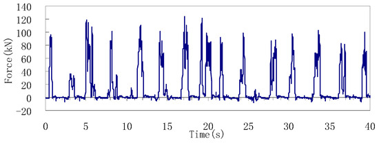
Figure 6.
Ice load recorded by the load panels on the JZ20-2 MUQ platform at 12:01 on 18 January 2001 [21].
3.1. Dynamic Ice Force Model for Conical Structures
Based on the analysis of these field measurements, the ice load acting on the conical surface is modeled as a sequence of independent isosceles triangular pulses. Each pulse represents one ice force cycle with random amplitudes F(i) and ice force periods Ti. The form of the pulses in this study is defined as an isosceles triangle. The interaction time between the ice and the cone is taken to be one-third of the ice force period. The random ice force function is as shown in Figure 7. The ice force function within one cycle can be defined by Equation (1) [21].

Figure 7.
Random ice load function for the narrow ice-breaking cone.
In the above formula, Ti represents the size of the ice force cycle for the cycle i. F0i denotes the amplitude of the ice force. Based on Equation (1), a random ice force function of any time length can be extended from Equation (2).
where N represents the number of ice force cycles that needs to be established, i = 0, . When i > 1, . Once the ice force cycles are extended to N cycles, the ice force amplitude F0i and the ice force period Ti are formed as two random sequences.
The ice force amplitude Fi and the ice force period Ti both follow a normal distribution, , . The mean value of the ice force amplitude is calculated using the Ralston formula, and the calculation formula for the mean value of the ice force period is by Equation (3).
3.2. Finite Element Simulation Analysis
To evaluate the structural response of the platform under the proposed random ice load model, finite element method (FEM) simulations were carried out using time-history analysis. The generated ice load sequences were applied as input to a transient dynamic simulation, allowing for detailed assessment of the platform’s acceleration response.
The FEM model was developed based on the structural dimensions provided in the original design drawings of the JZ20-2 NW platform. While the model was simplified for computational efficiency, key dynamic characteristics—such as modal frequencies—were preserved to ensure its accuracy in capturing realistic structural behavior. The final FEM model used in this study is shown in Figure 8.

Figure 8.
JZ20-2 NW platform finite element model.
The structural configuration includes the upper deck, a steel framing system, and an ice-breaking cone. The upper deck measures 12 m × 12 m and weighs approximately 250 tons. The waterline is located at 13.5 m, and the height of the main structural frame is 16 m. The cone structure is modeled with a maximum diameter of 6 m and double-box beam reinforcement.
To accurately simulate hydrodynamic and soil–structure interaction effects, additional modeling considerations were implemented: PIPE59 elements were used to account for added mass due to the surrounding water, PIPE16 beam elements were applied for the jacket structure, MASS21 point elements represented concentrated masses on the deck, and BEAM189 elements captured the response of key structural members. The equivalent pile length was set to six times the pile diameter to simulate foundation stiffness realistically.
Modal analysis confirmed that the fundamental natural frequency of the model is approximately 0.738 Hz, consistent with field measurements. This verifies the adequacy of the simplifications and the reliability of the model in reproducing real platform dynamics.
Upon completing the transient analysis, simulated acceleration time histories at key deck nodes were extracted in the direction of ice loading. These were then compared against measured acceleration responses from field monitoring under similar working conditions.
Figure 9 and Figure 10 present the measured and simulated acceleration time history curves, respectively. The comparison indicates that the model based on the random ice load function successfully captures the key features of the platform’s dynamic response, supporting the applicability of the load model in simulating real-world ice–structure interactions.
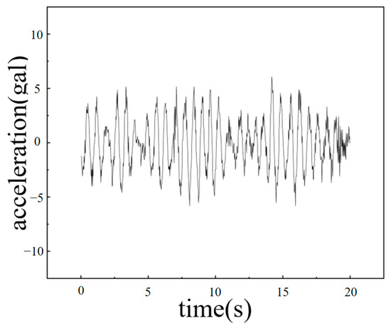
Figure 9.
The acceleration response time history curve of the measured data.

Figure 10.
The simulated acceleration response time history curve of the stochastic ice force model.
3.3. Analysis of Comparative Results
To validate the accuracy of the random ice force model, simulation results were compared with field monitoring data from the JZ20-2 NW platform under ten selected ice–structure interaction events. For each event, a corresponding ice load time history was generated using the random load function described in Section 3.1 and applied to the finite element model to calculate the platform’s acceleration response.
Table 1 summarizes the ice parameters for these events, including ice thickness, ice velocity, and the structural width at the waterline. For each case, the average and standard deviation of the measured acceleration response were extracted from the field data. Table 2 presents a comparison between these measured values and the acceleration responses simulated by the finite element model.

Table 1.
The ice condition data of the JZ20-2 NW platform under different conditions.
Table 2.
Comparison of the average amplitude and amplitude standard error between measured and simulated acceleration.
The results show that the simulated average acceleration magnitudes are generally higher than those observed in the field, with relative deviations ranging from 14% to 41%. The deviations in standard deviation are also within a reasonable range. Despite these differences, the overall trends and magnitudes of the simulated responses align well with the measured data, suggesting that the random ice force model effectively captures the key features of the platform’s dynamic response to ice loading.
Several factors may explain the observed discrepancies. The finite element model assumes uniform ice properties (e.g., thickness, strength, and density), while real sea ice exhibits significant variability due to factors such as temperature gradients, tidal effects, and microcracking. Additionally, field measurements may include noise from sources like wind, and sensor drift, which are not considered in the numerical model.
Overall, the comparison demonstrates that the random ice force model provides a reasonable approximation of the actual ice-induced responses. Further improvements could be achieved by refining the FEM model, introducing spatially variable ice properties, and incorporating ensemble simulation techniques to better capture the uncertainty in field conditions.
4. Random Load Inversion
In this section, a data-driven method for random ice load inversion is proposed based on the Temporal Convolutional Network (TCN) [22,23]. The approach reconstructs ice load time histories using measured structural response data, enabling indirect identification of dynamic ice loads acting on the platform.
The general workflow begins by using the ice load function described in Section 3.1 to generate input ice force time histories. These forces are applied to the finite element model to compute structural responses, which are then used to train the TCN model. The model is trained to learn the mapping from acceleration responses to corresponding ice loads. Once trained, the TCN can be used to perform inverse prediction of unknown ice loads based solely on observed acceleration data.
4.1. Basic Components of the Temporal Convolutional Network
TCN is a deep learning architecture designed specifically for modeling sequential data. It is particularly well-suited for tasks involving long-term temporal dependencies, such as dynamic load inversion based on time-series response data.
- Sequence Modeling
We highlight the nature of the sequence modeling task. Suppose that we are given an input sequence , …, , and wish to predict some corresponding outputs , …, at each time. The key constraint is that to predict the output for some time t, we are constrained to only use those inputs that have been previously observed: , …, . Formally, a sequence modeling network is any function that produces the following mapping:
Formally, a sequence modeling network is defined as any function that generates a mapping where depends only on , …, and does not rely on any “future” inputs , …, due to causal constraints. The goal of learning in the sequence modeling setting is to find a network that minimizes some expected loss between the actual outputs and the predictions, which means minimizing the value of Equation (5) [24].
- 2.
- Causal Convolutions
To preserve the temporal order of inputs and enforce the causality constraint, TCN uses causal convolutions. In a causal convolution, the output at time ttt is computed using only current and past input values, ensuring that no future information is introduced into the prediction. The causal convolutional neural network diagram is shown in Figure 11.
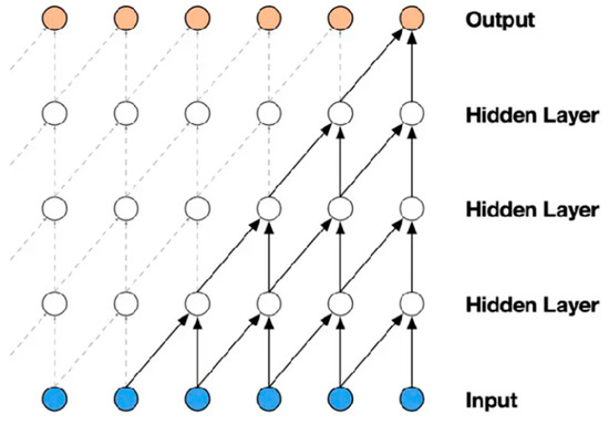
Figure 11.
The causal convolutional neural network diagram.
- 3.
- Dilated Convolutions
A simple causal convolution is only able to look back at a history with size linear in the depth of the network. This makes it challenging to apply the aforementioned causal convolution on sequence tasks, especially those requiring longer history. The solution is to employ dilated convolutions that enable an exponentially large receptive field [25]. Its primary purpose is to expand the receptive field of the convolutional kernel by introducing a dilation factor, thereby capturing long-range temporal dependencies while maintaining computational efficiency.
The structure diagram of TCN is as shown in Figure 12.

Figure 12.
The structure diagram of TCN.
- 4.
- Residual Connections
In TCN, residual connections are considered a key structural design aimed at enhancing the feature learning capability of the network and alleviating the potential gradient vanishing problem that may arise with increased depth. The basic idea of residual connections is that the input of a layer is directly added to its output, thereby providing a direct information pathway for the model. The core of residual connections lies in processing the input signal locally while retaining the original input information. Specifically, in TCN, consider an upstream input and the feature representation after a nonlinear transformation . By introducing a residual connection at a certain layer of the network, the output can be expressed as Equation (6). In this equation, is the output after the residual connection, and represents the features processed by the convolutional layers and activation functions. This design allows the model not only to learn complex representations through nonlinear transformations during the forward propagation but also to maintain the integrity of the input signal through the direct connection.
The residual module is as shown in Figure 13.

Figure 13.
Residual module.
4.2. Random Ice Load Inversion Process
The ice load inversion process includes four main steps. First, ice condition parameters such as ice thickness, velocity, and waterline width are collected and used to generate ice load time histories through the random ice force model. Second, these loads are applied to a finite element model of the JZ20-2 NW platform to simulate the corresponding acceleration responses. Third, the simulated acceleration data and the known ice loads are used to train a Temporal Convolutional Network (TCN) that learns the relationship between structural responses and applied loads. Finally, the trained model is evaluated using test data to confirm its ability to accurately predict unknown ice loads based on measured structural responses. This method combines simulation and machine learning to achieve efficient and accurate identification of random ice loads in offshore environments. The flowchart of the entire method is shown in Figure 14.
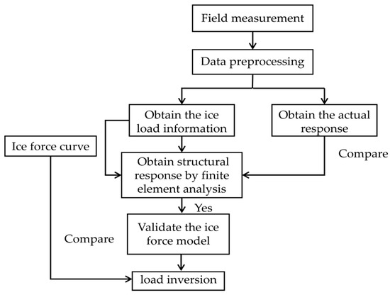
Figure 14.
Flow chart of random ice load inversion.
4.3. Ice Load Inversion
4.3.1. Model Training
The training dataset is built using 30 simulated events, each representing a different combination of ice thickness and velocity based on observed conditions in the Bohai Sea from 1990 to 2023. Each event includes 1200 time-series samples, where acceleration data serve as the input and the corresponding ice loads as the output. The dataset covers a wide range of ice conditions, including extreme cases, with ice thickness from 0.06 m to 0.5 m and ice velocity from 0.1 m/s to 0.5 m/s. Partial data for feature input are shown in Figure 15. In data processing, this study identifies and handles anomalies in ice load data using statistical methods. Initially, the 3σ rule is applied to exclude points more than three standard deviations from the mean. Then, the DBSCAN algorithm detects outliers in low-density areas to account for non-normal data distributions.
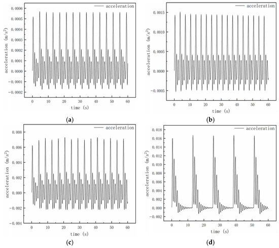
Figure 15.
Acceleration response under different conditions. (a) The first condition, (b) the second condition, (c) the third condition, and (d) the fourth condition.
Before conducting model training, this paper adopts the max.–min. normalization method to process the data, which can reduce the impact of different scales of data on model training. The mathematical formula is shown as Equation (7). is the actual value, and are the maximum and minimum values in the actual values, and is the normalized value.
The parameters of the TCN algorithm include kernel size, which determines the size of the convolutional filters applied to the input data; larger kernel sizes capture more context but may lose fine details. Dense units refer to the number of neurons in the fully connected layer, which determines the number of features that can be learned by that layer. The number of convolutional filters refers to the quantity of convolutional filters used in a convolutional layer, which determines the model’s ability to extract features from the input data. Each filter can learn different feature patterns, and increasing the number typically enhances the model’s performance; however, it also increases computational complexity and the risk of overfitting. Therefore, appropriate adjustments and validations should be made when selecting the number of filters. Dropout rate is employed to prevent overfitting by randomly setting a fraction of the input units to zero during training, which can enhance generalization. Learning rate is a critical hyperparameter that controls the size of the steps taken to update model weights during training. It significantly affects the convergence speed and overall performance of the model. A suitable learning rate helps the model to better find the optimal solution of the loss function.
For the selection of parameters in TCN learning models, there are many optimization algorithms available. Particle swarm optimization (PSO) is a swarm intelligence algorithm that is relatively simple, easy to implement, and does not require derivative computation for optimization problems [26]. After obtaining the structural response from the finite element simulation, the response is combined with external loads to form the dataset for training the TCN learning model. Prior to this, the parameters of the TCN model are optimized using a particle swarm optimization algorithm. Based on the reference literature [27,28] and relevant experimental experience, we selected relatively reasonable ranges for the parameters that could be optimized within a reasonable time frame. The optimization ranges and optimal parameters are detailed in Table 3. To prevent overfitting, five-fold cross-validation was used to validate the dataset.
Table 3.
Optimization parameter range and optimal parameters.
4.3.2. Model Verification
The model was trained using numerical simulation data. The partially identified loads on the training set and testing set are shown in Figure 16. The evaluation metric results are shown in Table 4. The evaluation metrics shown in Table 3 indicate that the R2 value of the TCN model on the training and testing sets under deterministic loads is close to 1. This indicates that the characteristics of the loads are accurately captured by the model, and the loads are effectively predicted and recognized. To accurately assess the stability of the R2 value, we employed the bootstrap method, performing 10,000 resampling iterations to calculate its 95% confidence interval. Specifically, we conducted multiple with-replacement samplings on both the training and test sets, recalculating the R2 value after each resampling to obtain its distribution and determine the confidence interval. The results strongly support the reliability of the model. The R2 on the training set is 0.821, with a 95% confidence interval of 0.798~0.837; on the test set, it is 0.808, with a 95% confidence interval of 0.782~0.825. From these data, it can be observed that the confidence intervals are relatively narrow. Such narrow intervals indicate smaller fluctuations of the R2 value across multiple resamples, suggesting high stability and statistical significance of the model’s performance. This also confirms that the reported R2 values are reliable. Using five-fold cross-validation, the results showed that the R2 values of the validation sets across different folds ranged from 0.793 to 0.807, with an average of 0.799. The mean R2 for the training sets was 0.821. These findings indicate that the model performs stably across different data splits. The cross-validation results further confirm that the proposed TCN model exhibits reliable generalization performance in ice load identification tasks and can effectively adapt to complex data variations encountered in real engineering scenarios.

Figure 16.
Load identification results. (a) Load identification results of training set and testing set, (b) Load identification results of testing set.
Table 4.
Evaluation metrics for random loads of TCN model.
The loss function of the prediction model uses the mean squared error (MSE) LMSE function, and its calculation formula is as Equation (8). is the number of samples. is the actual ice load value of the sample. is the predicted ice load value.
The loss function of the prediction model is as shown in Figure 17. The loss functions for the test and training sets show a decreasing trend with the increase in iteration count, and they gradually approach 0. This indicates that the model is able to fit the data well and has good generalization ability.
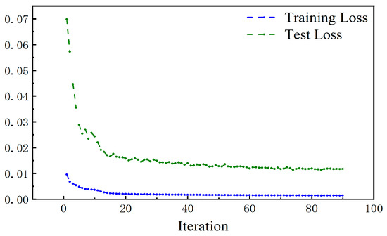
Figure 17.
Loss function of the prediction model.
In evaluating the model’s predictive performance, besides R2, this study analyzed the error distribution as shown in Table 5. Moreover, 95% of the absolute prediction errors are less than or equal to 21.3% and the kurtosis is 2.8, indicating a distribution close to normal with no significant outliers. This demonstrates that the prediction errors are within an acceptable range for engineering monitoring and that the distribution is stable. The TCN model meets the requirements for accuracy and stability in practical engineering applications.
Table 5.
Error distribution.
To verify the reliability and generalizability of the TCN model in load recognition tasks, load identification was performed under different ice thicknesses and ice speeds, with the identification results shown in Figure 18, and the evaluation metric R2 is presented in Table 6. The R values for the three operating conditions are close to 1. The results from this table indicate a strong correlation between the actual load and the load predicted by the TCN model. The effectiveness and reliability of the models in accurately predicting the target loads are confirmed by these results.
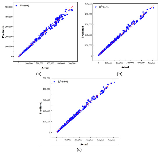
Figure 18.
Comparison of real load and predicted load. (a) The first condition, (b) the second condition, and (c) the third condition.
Table 6.
R2 under different working conditions.
This study only validated the model under three operating conditions. To better support the model’s generalizability, further validation over longer time spans and across more platforms would be desirable. However, there are significant objective challenges in extending the validation. From the platform resource perspective, acquiring data from additional platforms faces great difficulties. Offshore platforms are widely distributed and operate in complex environments; differences in monitoring systems, data formats, and sampling frequencies across platforms make data integration extremely challenging. Regarding model resources, we currently lack additional suitable models for reference and comparison validation. Developing new models requires substantial expertise and computational resources, as well as considerations of the complex platform structures and ice loads. Furthermore, obtaining relevant offshore data is very difficult.
4.3.3. Difference Analysis
Although the TCN model shows strong performance on simulated data, differences may arise when applied to real-world scenarios. One key reason is that the FEM simulations are based on idealized assumptions—such as uniform ice thickness and consistent material properties—whereas real sea ice exhibits spatial variability influenced by temperature, salinity, and environmental conditions. The range of conditions used for training may also be limited; for example, extreme or irregular ice behaviors such as sudden changes in thickness or multi-directional flows may not be well represented.
These factors can reduce the model’s adaptability when applied to more complex or unmodeled conditions. In particular, under highly dynamic or non-uniform ice loading, the TCN model may struggle to fully capture all features of the real ice load response, leading to prediction errors.
Improving the model’s generalization ability may require incorporating more diverse real-world datasets, refining the simulation process, and exploring ensemble learning approaches to handle a wider range of ice–structure interaction scenarios.
4.4. Comparative Analysis with Traditional Sequence Models
To further evaluate the performance of the TCN model, a comparative analysis was conducted against a traditional Deep Neural Network (DNN) model. Both models were trained and tested using the same dataset, which includes structural response and ice load data under various ice thickness and velocity conditions. The data split ratio was also kept consistent, with 80% for training and 10% each for validation and testing.
Figure 19 shows the loss curve of the DNN model, and Table 7 presents the evaluation results. The DNN model achieved an R2 of 0.78 on both the training and test sets, which is noticeably lower than the TCN’s performance. While DNNs are effective for general regression tasks, they do not explicitly account for temporal dependencies in sequential data, which limits their accuracy in time-series load identification.

Figure 19.
Loss function of the DNN prediction model.
Table 7.
Evaluation metrics for random loads of DNN model.
Under the same conditions shown in Table 6, the TCN model consistently outperformed the DNN, especially in cases involving large fluctuations in ice load. TCN more accurately followed the real trend in the ice load time series, while DNN produced higher deviations, particularly under complex or extreme loading conditions. The higher R2 values of the TCN (reaching up to 0.996) confirm its superior ability to model dynamic, time-dependent ice loads.
This comparison highlights the advantages of TCN in sequence modeling tasks related to offshore structural responses, showing that it offers better accuracy, stability, and generalization than traditional deep learning models in the context of ice load identification.
Load identification was performed under the same ice speed and ice thickness as in Table 6, and the recognition results of the DNN model are shown in the Figure 20. From the accuracy perspective, TCN demonstrates higher performance than DNN on both training and testing sets. It captures the trend in ice load variations more precisely, enabling more accurate identification of ice load data under different working conditions. This advantage of TCN is especially evident when dealing with complex ice scenarios. For example, under varying ice thickness and speed conditions, when the fluctuations are large, predictions of TCN deviations from actual values are significantly smaller than those of DNN. Regarding R2 values, TCN approaches 0.99 across various complex conditions, while values of DNN are comparatively lower. This indicates that the TCN model has a better fitting performance and can more accurately reflect the true characteristics of ice load.

Figure 20.
Comparison of real load and predicted load of DNN model. (a) The first condition, (b) the second condition, and (c) the third condition.
Although this study validates the effectiveness of the TCN model in dynamic ice load identification, the pathway from theory to practical engineering application remains to be clearly defined. First, a real-time data acquisition and preprocessing system must be established, integrating accelerometer responses and ice condition parameters obtained through sensor networks in real time. The model should be optimized to enhance efficiency, meeting the low-latency requirements for real-time on offshore platforms. Finally, a closed-loop feedback system should be developed to compare real-time prediction results with on-site monitoring data, enabling dynamic updates of model parameters to adapt to the time-varying characteristics of the sea ice environment. There are multiple challenges in transitioning from theory to practical engineering application. Regarding data acquisition and processing, harsh offshore conditions can interfere with sensor operation, leading to noise, delays, or data loss. Additionally, the data collected by different sensors may have accuracy differences and synchronization issues, complicating model input. Concerning the model itself, its generalization ability may be insufficient under extreme ice conditions, and changes in complex ice scenarios can impact its stability and accuracy. In terms of computational resources, the limited processing power and storage capacity of offshore platform equipment make it difficult to meet the demands of complex model calculations and data storage while also considering energy consumption issues.
5. Conclusions
This study presents a data-driven method for identifying random ice loads on conical offshore platforms using a Temporal Convolutional Network (TCN). By integrating a stochastic ice force model, finite element simulations, and deep learning, a complete inversion framework is developed for dynamic load identification based on structural responses. The main conclusions are summarized as follows:
- (1)
- A random ice load model was established based on field observations of ice–cone interaction. The model represents ice loading as a sequence of triangular pulses with randomly distributed amplitudes and periods. Finite element analysis confirmed that the model accurately reproduces the dynamic behavior of ice loading, with simulation results closely matching field measurements.
- (2)
- A TCN-based inversion method was proposed to identify time-varying ice loads from structural response data. The model architecture—including causal and dilated convolutions with residual connections—enables effective capture of long-term temporal patterns. Particle swarm optimization (PSO) was used to optimize hyperparameters, improving the model’s accuracy and generalization.
- (3)
- The TCN model was trained using ice load and structural response data generated from stochastic ice force functions and finite element simulations. The model’s performance on the training and test sets demonstrates that the TCN can accurately identify ice loads and exhibits a high goodness of fit (R2 value close to 1).
- (4)
- The model performed well under a range of ice thickness and velocity conditions, showing strong correlation between predicted and actual loads. Compared with a traditional Deep Neural Network (DNN), the TCN model demonstrated superior performance in terms of accuracy, especially under complex and fluctuating ice conditions.
Overall, this study demonstrates that the TCN model is a reliable and efficient tool for dynamic ice load identification on conical offshore platforms. The approach leverages the strengths of simulation and machine learning to overcome the limitations of traditional methods, offering a scalable solution for structural monitoring in ice-prone regions.
Currently, the method is primarily validated using simulated and limited field data. In future work, the model’s generalization can be further improved by incorporating more real-world monitoring data from multiple platforms and longer time spans. Moreover, deployment in real-time systems could enable online ice load monitoring and early warning for offshore operations.
Author Contributions
Conceptualization, W.L. and Y.Q.; methodology, Y.G. (Ya Guo); software, S.L.; validation, Y.G. (Yang Gao) and W.L. All authors have read and agreed to the published version of the manuscript.
Funding
This research was funded by the GJYC program of Guangzhou (Grant No. 2024D03J0022).
Data Availability Statement
No new data were created or analyzed in this study.
Conflicts of Interest
Authors Wei Li, Shuzhao Li and Yang Gao were employed by the company CNOOC Research Institute Co., Ltd. The remaining authors declare that the research was conducted in the absence of any commercial or financial relationships that could be construed as a potential conflict of interest.
References
- Li, W.; Yin, H.; Fu, D.; Sun, S. Key Issues and Suggestions for Ice-Resistant Design of Offshore Platform Structures in China. China Offshore Oil Gas 2024, 36, 199–211. [Google Scholar]
- Wang, Y. A new method for long-term safety analysis of marine structures. J. S. Afr. Inst. Civ. Eng. 2024, 65, 10–22. [Google Scholar] [CrossRef]
- De Koker, N.; Bekker, A. Assessment of ice impact load threshold exceedance in the propulsion shaft of an ice-faring vessel via Bayesian inversion. Struct. Health Monit. 2022, 21, 757–769. [Google Scholar] [CrossRef]
- Ramadhani, A.; Khan, F.; Colbourne, B.; Ahmed, S.; Taleb-Berrouane, M. Resilience assessment of offshore structures subjected to ice load considering complex dependencies. Reliab. Eng. Syst. Saf. 2022, 222, 108421. [Google Scholar] [CrossRef]
- Erceg, S.; Erceg, B.; von Bock und Polach, F.; Ehlers, S. A simulation approach for local ice loads on ship structures in level ice. Mar. Struct. 2022, 81, 103117. [Google Scholar] [CrossRef]
- Li, W.; Yin, H.; Sun, J.; Gao, Y.; Zhang, M. A tentative ice force formula for vertical piles in Bohai Sea based on model tests. Ocean. Eng. 2025, 322, 120522. [Google Scholar] [CrossRef]
- Li, W.; Gao, Y.; Sun, S. Research on the Ice Force Masking Effect of an Eight-Leg Jacket Platform Based on Model Tests. Shipbuild. China 2024, 65, 37–52. [Google Scholar]
- Kong, S.; Cui, H.; Tian, Y.; Ji, S. Identification of ice loads on shell structure of ice-going vessel with Green kernel and regularization method. Mar. Struct. 2020, 74, 102820. [Google Scholar] [CrossRef]
- Zhang, M.; Qiu, B.; Qu, X.; Shi, D. Improved C-optimal design method for ice load identification by determining sensor locations. Cold Reg. Sci. Technol. 2020, 174, 103027. [Google Scholar] [CrossRef]
- Chen, Z.; Chan, T.H.T.; Yu, L. Comparison of regularization methods for moving force identification with ill-posed problems. J. Sound Vib. 2020, 478, 115349. [Google Scholar] [CrossRef]
- Yang, W.; Wang, S. Modal Parameters Identification of a Real Offshore Platform from the Response Excited by Natural Ice Loading. China Ocean Eng. 2020, 34, 558–570. [Google Scholar] [CrossRef]
- Chen, Z.; Sun, P.; Chan, T.H.T.; Yu, L. Ill-Posedness Determination of Moving Force Identification and Parameters Selection for Regularization Methods. Int. J. Struct. Stab. Dyn. 2021, 21, 2150114. [Google Scholar] [CrossRef]
- Umamahesan, A.; Babu, D.M.I.; Association for Computing Machinery. From Zero to AI Hero with Automated Machine Learning. In Proceedings of the 26th ACM SIGKDD International Conference on Knowledge Discovery and Data Mining (KDD), San Diego, CA, USA, 23–27 August 2020; Association for Computing Machinery: New York, NY, USA, 2020. [Google Scholar]
- Weng, W.-D. Decomposition-Based Optimal Temporal Convolutional Networks Applied for Load Forecasting. In Proceedings of the 2022 International Conference on Smart City and Green Energy (ICSCGE), Hong Kong, China, 19–21 November 2022. [Google Scholar]
- Shan, D.; Yao, K.; Zhang, X. Sequential Learning Network with Residual Blocks: Incorporating Temporal Convolutional Information into Recurrent Neural Networks. IEEE Trans. Cogn. Dev. Syst. 2024, 16, 396–401. [Google Scholar] [CrossRef]
- Wu, P.; Sun, J.; Chang, X.; Zhang, W.; Arcucci, R.; Guo, Y.; Pain, C.C. Data-driven reduced order model with temporal convolutional neural network. Comput. Methods Appl. Mech. Eng. 2020, 360, 112766. [Google Scholar] [CrossRef]
- Xu, C.; Zhao, P.; Liu, Y.; Xu, J.; Sheng, S.; Cui, Z.; Zhou, X.; Xiong, H. Recurrent Convolutional Neural Network for Sequential Recommendation. In Proceedings of the World Wide Web Conference (WWW ‘19), San Francisco, CA, USA, 13–17 May 2019; Association for Computing Machinery: New York, NY, USA, 2019. [Google Scholar]
- Sinsabvarodom, C.; Leira, B.J.; Høyland, K.V.; Næss, A.; Samardžija, I.; Chai, W.; Komonjinda, S.; Chaichana, C.; Xu, S. On Statistical Features of Ice Loads on Fixed and Floating Offshore Structures. J. Mar. Sci. Eng. 2024, 12, 1458. [Google Scholar] [CrossRef]
- Huang, Y.; Yu, S.; An, T.; Wang, G.; Zhang, D. Investigating the Ice-Induced Fatigue Damage of Offshore Structures by Field Observations. J. Mar. Sci. Eng. 2023, 11, 1844. [Google Scholar] [CrossRef]
- Ralston, T.D. Ice Force Design Considerations for Conical Offshore Structures. In Proceedings of the 4th International Conference on Port and Ocean Engineering Under Arctic Conditions (POAC 77), St. John’s, NL, Canada, 26–30 September 1977. [Google Scholar]
- Yan, Q.; Yue, Q.; Bi, X.; Tuomo, K. A random ice force model for narrow conical structures. Cold Reg. Sci. Technol. 2006, 45, 148–157. [Google Scholar] [CrossRef]
- Chen, F.; Zhang, Y.; Chen, L.; Meng, X.; Qi, Y.; Wang, J. Dynamic traveling time forecasting based on spatial-temporal graph convolutional networks. Front. Comput. Sci. 2023, 17, 176615. [Google Scholar] [CrossRef]
- Zhou, Y.; Chen, Z.; Xie, A. Temporal Attention Convolutional Neural Networks Based on LSTM-Encoder for Time Series Forecasting. In Proceedings of the 2023 International Conference on Networks, Communications and Intelligent Computing (NCIC), Suzhou, China, 17–19 November 2023; pp. 51–54. [Google Scholar]
- Bai, S.; Kolter, Z.; Koltun, V. An Empirical Evaluation of Generic Convolutional and Recurrent Networks for Sequence Modeling. arXiv 2018, arXiv:1803.01271. [Google Scholar]
- van den Oord, A.; Dieleman, S.; Zen, H.; Simonyan, K.; Vinyals, O.; Graves, A.; Kalchbrenner, N.; Senior, A.; Kavukcuoglu, K. WaveNet: A Generative Model for Raw Audio. arXiv 2016, arXiv:1609.03499. [Google Scholar]
- Yang, X.; Li, H. Evolutionary-state-driven multi-swarm cooperation particle swarm optimization for complex optimization problem. Inf. Sci. 2023, 646, 119302. [Google Scholar] [CrossRef]
- Lea, C.; Flynn, M.D.; Vidal, R.; Reiter, A.; Hager, G.D. Temporal Convolutional Networks for Action Segmentation and Detection. In Proceedings of the IEEE Conference on Computer Vision and Pattern Recognition, Honolulu, HI, USA, 21–26 July 2017. [Google Scholar]
- Yang, L.; Koprinska, I.; Rana, M. Temporal Convolutional Attention Neural Networks for Time Series Forecasting. In Proceedings of the 2021 International Joint Conference on Neural Networks (IJCNN), Shenzhen, China, 18–22 July 2021. [Google Scholar]
Disclaimer/Publisher’s Note: The statements, opinions and data contained in all publications are solely those of the individual author(s) and contributor(s) and not of MDPI and/or the editor(s). MDPI and/or the editor(s) disclaim responsibility for any injury to people or property resulting from any ideas, methods, instructions or products referred to in the content. |
© 2025 by the authors. Licensee MDPI, Basel, Switzerland. This article is an open access article distributed under the terms and conditions of the Creative Commons Attribution (CC BY) license (https://creativecommons.org/licenses/by/4.0/).