Seafloor Stability Assessment of Jiaxie Seamount Group Using the “Weight-of-Evidence” (WoE) Method, Western Pacific Ocean

Abstract

The deep sea is gradually being exploited, yet research on the stability of the deep seabed is scarce. In this study, the seafloor stability of the Jiaxie Seamount Group in the western Pacific Ocean was assessed using the weight-of-evidence (WoE) method based on seafloor topographic data. Slope failure features were identified by analyzing multibeam bathymetric data, revealing 21 failure zones and multiple debris accumulation areas. Topographic factors, such as water depth, slope, slope direction, planar curvature, profile curvature, and ruggedness, were selected as assessment indicators. These indicators were reclassified as evidence factors, and a WoE model was constructed to assess the failure probability in the study area. A stability zoning map indicated that over 93% of the area had high stability. In comparison, areas with low and very low stability comprised less than 4%, mainly located on steep ridges and rugged slopes. The model’s performance was validated through an ROC curve, yielding an AUC value of 0.929, indicating a high predictive capability. This study presents a statistical framework for assessing the stability of deep-sea floors and provides theoretical support for upcoming seabed mining and deep-sea engineering endeavors, despite limitations due to data constraints and dependence on visually interpreted slope failure zones.

1. Introduction

Seamounts are crucial ecological components within marine ecosystems, and they are capable of influencing ocean currents and material transport. They modify the direction and velocity of water currents, thereby facilitating the upwelling and circulation of nutrients. Consequently, they play a significant role in facilitating energy flow and material circulation throughout the entire marine ecosystem [1,2]. The unique topography and geomorphology of seamounts create unique conditions that enrich nutrients on the seabed, making it an ideal habitat for marine organisms [3,4,5]. However, seamount slope failure can cause severe damage to the habitats of these organisms. At the same time, the seamounts in the western Pacific are abundant in polymetallic nodules and crusts [6,7], and several countries have developed plans to achieve the commercial exploitation of seabed mineral resources within the next decade [8]. Evaluating the stability of seamounts is a prerequisite for the deployment of mining systems, and it can consequently provide a scientific foundation for deep-sea environmental protection and mineral resource development.

Deep-sea exploration technology is continuing to develop with increasing accuracy, efficiency, and intelligence. Not only has this trend significantly accelerated scientific research in areas such as seabed topography, ecosystems, and resources, but it has also provided key technical support for ocean engineering, resource development, and environmental protection [9]. As key technologies such as multiplatform cooperative operation, system integration, and intelligent control continue to advance, deep-sea exploration equipment will become deployable on a large scale in the deep sea, and deep-sea engineering projects will be further developed [10]. Seamount stability assessment is crucial for site selection and safety assessment in deep-sea engineering.

Currently, research on seafloor stability primarily focuses on offshore regions, with most of it being related to hydrate extraction [11,12]. Research on seamount slope failure mainly focuses on the qualitative description of the failure phenomenon. Deplus described submarine evidence for large-scale debris avalanches in the Lesser Antilles Arc using a marine geophysical survey [13]. Saint-Ange posited that coastal and submarine instabilities are the primary processes shaping a volcano’s submarine morphology, as evidenced by high-resolution multibeam and backscatter data, deep-water photographs, side-scan imagery, and Kullenberg piston cores [14]. Chang’s research on mapping submarine landslides around the volcanic islands of the Azores was primarily based on high-resolution echo-sounder data [15]. However, there is a significant dearth of research on the assessment of the seafloor stability of deep-sea seamounts, primarily due to two reasons: the difficulty in obtaining relevant data and the immaturity of research methodologies. Most probabilistic assessments of land slope stability employ statistical modeling, where factors related to slope failure are examined in a multivariate statistical analysis to study the correlation between instability and its influencing factors [16,17,18,19]. As artificial intelligence technology advances, machine learning methods have been increasingly integrated into the field of slope stability assessment, significantly enhancing assessment efficiency and reducing workload [20,21,22,23]. However, machine learning requires substantial environmental data to construct datasets for slope stability assessment, making it challenging to support research on machine learning methods due to the current amount of seamount data. Dondin employed the limit equilibrium method to analyze slope stability by measuring the physical properties of rock at the Kick-’em-Jenny submarine volcano [24]. It is difficult to comprehensively determine the physical parameters of the rocks of deep-sea seamounts, and it is difficult to comprehensively evaluate the stability of seamounts using the above methods. Therefore, there is an urgent need to develop relevant research methods for the stability evaluation of seamounts.

In this study, the seafloor stability of the Jiaxie Seamount Group was assessed by employing the weight-of-evidence method, a statistical technique, based on seamount topographic data. The aim was to provide foundational research insights for the protection of deep-sea environments, the development of mineral resources, and the construction of deep-sea engineering projects.

2. Geological Background

Most seamounts within the Magellan Seamount Group originated during the Late Jurassic to Early Cretaceous period. Their basal basalts are in good continuity with the Middle and Late Jurassic uplifted basalts in the surrounding ocean basins [25]. The sedimentary sequences in the eastern and western guyots consist of rock complexes of similar ages and types, mainly carbonate sedimentary rocks, such as reef, oolitic, and planktonic limestones [26,27]. The seamounts’ basement consists of volcanic rocks originating from a mix of Early Cretaceous effusive rocks, characterized by the tholeiite–alkali basalt association. During the Aptian–Cenomanian period, reef, oolitic, and planktonic limestones developed on the summits of the seamounts, and these formations are rich in fossilized bivalves, corals, and sea urchins. Following the Cenomanian order, seamount subsidence intensified and entered a phase of deep-water deposition, with planktonic foraminiferal limestones becoming the dominant lithology, replacing the reef limestones. Following the Quaternary period, the seamount summits were blanketed with loose carbonate deposits, suggesting that the seamounts had transitioned into a deep-water environment.

The Jiaxie Seamount Group, the subject of this study, is part of the eastern section of the Magellan Seamount Group (Figure 1). It is situated within the range of 156°~157°22′ E and 12°~13°17′ N. The Jiaxie Seamount Group comprises the Weijia, Weizhen, and Weixie Guyots. It has a basal water depth of approximately 5900 m, with the top platform distributed at water depths ranging from 1350 to 2000 m and the edges distributed at depths from 1600 to 2600 m. The eastern part of the summit platform of the Weijia Guyot is approximately square (35 km × 35 km), and the western part is L-shaped (10 km~15 km wide), with a total area of about 1630 km². The guyot has four radial ridges extending eastward, southward, southwestward, and northward. At the end of the southwest ridge lies the Weizhen Guyot, surrounded by six smaller ridges. The southern seamount is the Weixie Guyot, which is nearly dome-shaped, with only one radial ridge in its northeastern corner. Most of the summit platform is covered by loose carbonate deposits, and the bedrock outcrops at the edges exhibit erosional features. Carbonate–clay clastic fans are widely developed at depths below 3000 m [28,29].

3. Data and Methods

3.1. Data Acquisition and Processing

The data for this study were derived from deep-water multibeam data collected during the China Dayang 66, 80, and 86 cruises to the seamounts in the western Pacific Ocean, supplemented by bathymetry data from GEBCO [30].

Multibeam bathymetric data from a single source cannot fully represent the topographic characteristics of the entire study area, necessitating the integration of bathymetry data from various sources, a process referred to as multisource data fusion [32]. If the differences in resolution and depth between different bathymetry datasets are small, then the data can be directly spliced and fused; however, if they are significant, then the data must be corrected for these discrepancies after unifying the resolution, and then they must be spliced and fused.

Difference correction is the process of reducing the elevation discrepancies between terrain data from various sources. The conventional method for correcting elevation differences involves calculating the average value of the elevation discrepancies in the overlapping region between the base terrain data and the data requiring correction. This average is then applied to the data that need to be corrected [29]. However, difference correction using the method described above does not highlight the details of the terrain data in non-overlapping areas. The difference correction method proposed in this paper involves predicting the height differences across all the bathymetry data to be calibrated. This is achieved by calculating the height differences in the overlapping areas of different bathymetry data and using the depth and slope of the bathymetry data to be calibrated as explanatory variables, employing the Random Forest algorithm. The splicing and fusion of different terrain data require the boundary transitions to be natural [33]. The splicing boundary is typically processed using filtering methods to ensure the continuity of the boundary. In this study, median filtering and mean filtering were applied to process the boundary of the fused data, thereby obtaining complete bathymetry data for the study area.

In this study, Caris 11.4 was used to process the multibeam line survey data obtained from the previous years’ voyages in the study area. After processing, most of the bathymetry data for the study area were obtained. Using the processed bathymetry data as a baseline, a public dataset was subjected to difference correction. Subsequently, the difference-corrected public dataset was supplemented with blank areas in the study region, resulting in more complete bathymetry data for the study area.

3.2. Failure Zone Identification

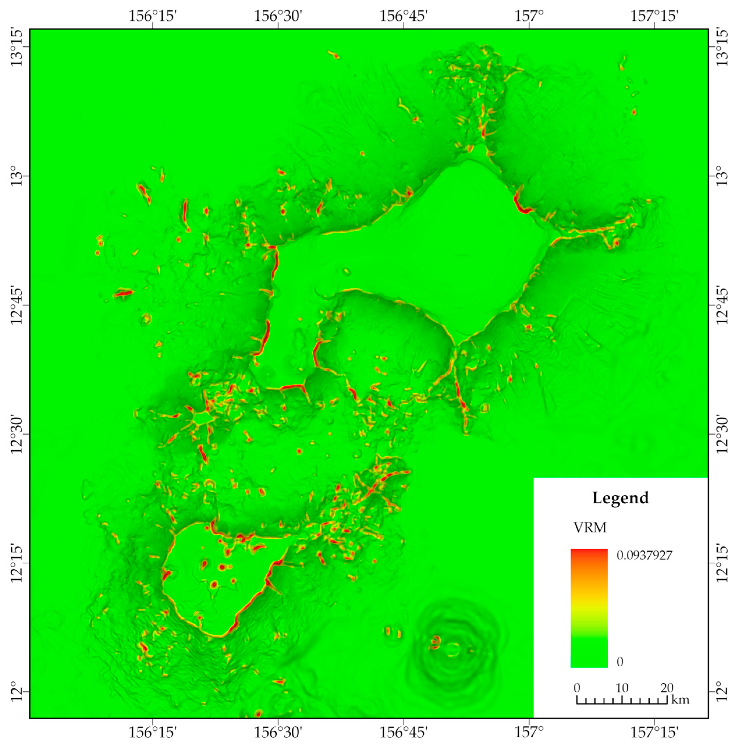
Upon the occurrence of failure in submarine slopes, the sequence of geotechnical processes—from the initiation of movement to the final depositional phase—can give rise to a variety of geomorphic patterns [34,35]. These geomorphic patterns are recognized based on their structural characteristics, which differ from those of the surrounding seafloor geomorphology. Typical features of slope failure include elements such as the curved recessed scarp, the sidewall, the sliding surface, and the raised toe of the slope. Multibeam bathymetric 3D maps can only depict the main scarp, the sidewalls, and portions of the landslide body; they cannot directly display the subsurface portion of the landslide. In localized areas of submarine slopes, landslide erosion may occur if there is a significant change in the slope, particularly when a distinctive feature, such as the curved main scarp, is steeper than the surrounding adjacent areas [36,37,38]. Meanwhile, we found that the VRM metrics, which characterize ruggedness, are more effective in identifying the main scarp and sidewall features of slope failure. The top of the main scarp and the upper part of the sidewall exhibited higher VRM values (Figure 2). Thus, in this study, the main scarp location of the slope failure was initially identified using a map of the VRM calculation results. Subsequently, the slope failure zones were further delineated by integrating the seamount slope map with the bathymetric map.

3.3. Assessment Indicator System

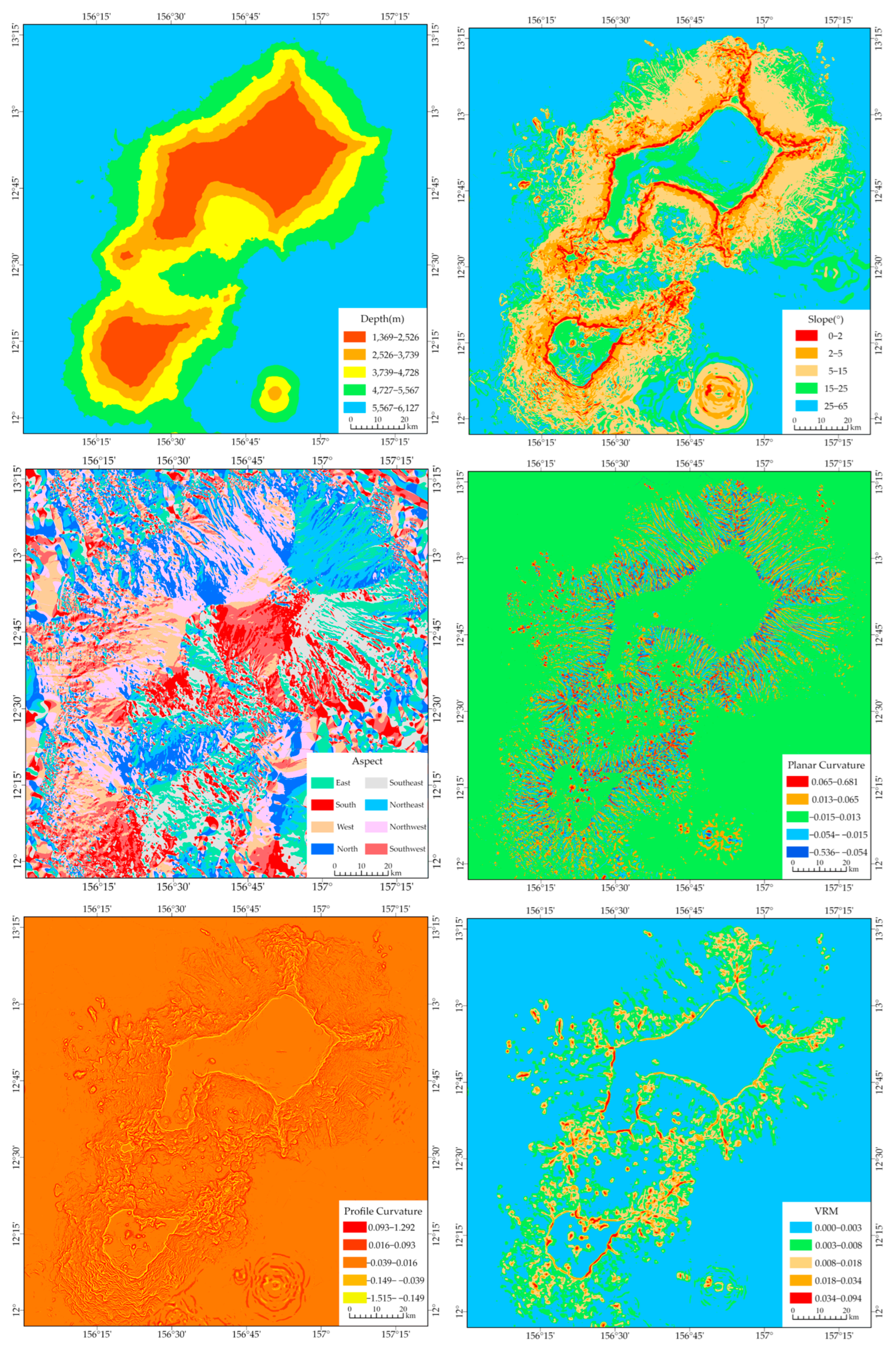
The seamounts in the western Pacific Ocean are located in deep and distant oceanic regions, making detailed seafloor environmental data difficult to obtain. Therefore, in this study, the stability assessment of the Jiaxie Seamount Group is mainly based on topographic impact factors. Based on the multibeam bathymetry datasets, six topographic factors are extracted: water depth, slope, aspect, planar curvature, profile curvature, and the ruggedness index VRM (Figure 3). The water depth is usually obtained directly from multibeam bathymetric data, which can reflect the distribution characteristics of sedimentary layers to some extent. The slope indicates the inclination of the surface, which is the angle between the tangent plane and the horizontal ground at a specific point. This angle can be calculated based on the rate of change in the regional depth. The steeper the area, the greater the degree of influence of gravity. The aspect indicates the change in the direction of the slope, which is the angle formed by the north direction of a specific point on the surface and the projection line obtained from the normal direction of its tangent plane on the horizontal plane. This is commonly used to analyze the erosion effects of ocean currents. The influence of water flow on slopes is closely related to the aspect. The planar curvature indicates the extent of contour curvature and describes the aggregation or dispersion characteristics of water flow in the horizontal direction, reflecting the intensity of the water flow. The profile curvature describes the degree of curvature of the terrain in the direction of the slope, reflecting the acceleration and deceleration effects of erosion or deposition. The ruggedness quantifies the degree of surface roughness of the terrain, reflecting geological stability or biological habitat complexity. In this study, the VRM index is used to characterize ruggedness. Areas with a higher VRM value tend to exhibit a greater resistance to seawater and are generally relatively less stable.

3.4. Weight-of-Evidence Modeling

The weight-of-evidence method is a statistical technique used to assess the relationships between categorical variables and target variables, and it is commonly applied in credit scoring models, risk management, and feature engineering [39,40]. It assesses the predictive capacity of a variable for a target event by transforming raw data into weight values. The method primarily relies on Bayes’ theorem for statistical prediction, under the assumption that each evidence factor is independent of the others given the conditions of the target event [41]. The core concept involves calculating the posterior probability to identify high-potential regions by quantifying the contribution weights of various evidence factors to the target event.

3.4.1. A Priori Probability Calculation

When assessing the stability of seamounts based on the weight-of-evidence method, the six extracted topographic factors are used as assessment indicators, and the identification results of slope failure zones are used as target events. Each assessment indicator is categorized into various evidence factors, followed by the calculation of a priori probabilities. This process specifically encompasses the distribution probability of the failure phenomenon and the evidence factors. In the assessment indicator grid, F represents the failure unit, and E represents the evidence factor. The distribution probability of the failure phenomenon P(F) and that of the evidence factor P(E) can be calculated individually through pixel statistics. The pixel statistics are based on the identification results of slope failure zones in the bathymetry map. The calculation formulas are as follows:

$$P\left(F\right)=A_F/A_L$$

(1)

$$P\left(E\right)=A_E/A_L$$

(2)

where A_F denotes the number of failure pixels in the assessment area, A_E denotes the number of evidence factor pixels, and A_L denotes the number of assessment area total pixels.

3.4.2. A Posteriori Probability and Odds Calculation

With the known distribution probability of the failure phenomenon and the evidence factor, the process of calculating the failure probability in the evidence factor ($P\left(F|E\right)$), the non-failure probability in the evidence factor ($P\left(\overline{F}|E\right)$), the failure probability in the non-evidence factor ($P\left(F|\overline{E}\right)$), and the non-failure probability in the non-evidence factor ($P\left(\overline{E}|\overline{F}\right)$) is known as a posteriori probability calculation. The calculation formulas are as follows:

$$P\left(F|E\right)=P\left(E\bigcap F\right)/P\left(E\right)=P\left(E|F\right)\times P\left(F\right)/P\left(E\right)$$

(3)

$$P\left(\overline{F}|E\right)=P\left(E\bigcap \overline{F}\right)/P\left(E\right)=P\left(E|\overline{F}\right)\times P\left(\overline{F}\right)/P\left(E\right)$$

(4)

$$P\left(F|\overline{E}\right)=P\left(\overline{E}\bigcap F\right)/P\left(\overline{E}\right)=P\left(\overline{E}|F\right)\times P\left(F\right)/P\left(\overline{E}\right)$$

(5)

$$P\left(\overline{F}|\overline{E}\right)=P\left(\overline{E}\bigcap \overline{F}\right)/P\left(\overline{E}\right)=P\left(\overline{E}|\overline{F}\right)\times P\left(\overline{F}\right)/P\left(\overline{E}\right)$$

(6)

The ratio of the probability of an event occurring to the probability of it not occurring is referred to as the odds in statistics. The odds better represent the magnitude of the likelihood of an event occurring than the probability itself. By dividing Formula (3) by Formula (4) and by dividing Formula (5) by Formula (6), we can compute the ratio of the failure probability to the non-failure probability for both the evidence factor and the non-evidence factor. This yields the a posteriori odds for the evidence factor and the non-evidence factor, respectively. The calculation formulas are as follows:

$$O\left(F\right)=P\left(F\right)/\left(1-P\left(F\right)\right)$$

(7)

$$O\left(F\right)=P\left(F\right)/\left(1-P\left(F\right)\right)$$

(8)

$$O\left(F|\overline{E}\right)=P\left(\overline{E}|F\right)/P\left(\overline{E}|\overline{F}\right)\times O\left(F\right)$$

(9)

By taking the natural logarithm of both sides of Formulas (8) and (9) and then transforming the formulas, the resulting variant formulas are as follows:

$$\ln O\left(F|E\right)=\ln \left(P\left(E|F\right)/P\left(E|\overline{F}\right)\right)+\ln O\left(F\right)$$

(10)

$$\ln O\left(F|\overline{E}\right)=\ln \left(P\left(\overline{E}|F\right)/P\left(\overline{E}|\overline{F}\right)\right)+\ln O\left(F\right)$$

(11)

3.4.3. Weight-of-Evidence Calculation

The weight $W_j^{+}$ is the ratio of the distribution probability of the failure phenomenon and the non-failure phenomenon in the presence of the evidence factor, and the weight $W_j^{-}$ is the ratio of the distribution probability of the failure phenomenon and the non-failure phenomenon in the absence of the evidence factor. When there is a positive correlation between the evidence factor and the occurrence of the failure phenomenon, the weight value is $W_j^{+}>0$, $W_j^{-}<0$, indicating that the evidence factor plays a significant role in promoting the occurrence of the failure phenomenon. When there is a negative correlation between the evidence factor and the occurrence of the failure phenomenon, the weight value is $W_j^{+}<0$, $W_j^{-}>0$, indicating that the promotion of the evidence factor on the occurrence of the failure phenomenon is not obvious. No correlation between the evidence factor and the occurrence of the failure phenomenon indicates that the failure probability for the evidence factor is 0, meaning that no failure phenomenon occurs in the evidence factor. The calculation formulas are as follows:

$$W_j^{+}=\ln {\displaystyle \frac{P\left(E|F\right)}{P\left(E|\overline{F}\right)}}=\ln {\displaystyle \frac{\left(A_j\bigcap A_F\right)/A_F}{\left(A_j\bigcap \overline{A_F}\right)/\overline{A_F}}}$$

(12)

$$W_j^{-}=\ln {\displaystyle \frac{P\left(\overline{E}|F\right)}{P\left(\overline{E}|\overline{F}\right)}}=\ln {\displaystyle \frac{\left(\overline{A_j}\bigcap A_F\right)/A_F}{\left(\overline{A_j}\bigcap \overline{A_F}\right)/\overline{A_F}}}$$

(13)

where $A_F$ denotes the number of failure pixels, $\overline{A_F}$ denotes the number of non-failure pixels, $A_j$ denotes the number of pixels of each evidence factor, and $\overline{A_j}$ denotes the number of pixels of each non-evidence factor.

The difference between positive and negative weights is referred to as the relative or sensitivity coefficient. Compared to positive or negative weights, the relative coefficient takes into account both the presence and absence of evidence weights, more accurately reflecting the influence of weight-of-evidence factors on the failure phenomenon. The greater the value of the relative coefficient, the greater the degree of influence of the evidence factor on the failure phenomenon. The total weight of evidence considers the cumulative impact of various evidence factors, including the relative coefficients of these factors and the sum of the negative weights. The calculation formulas are as follows:

$$C=W^{+}-W^{-}$$

(14)

$$W_{ij}=C_{ij}+\sum _j^y{W}_{ij}^{-}$$

(15)

3.4.4. Failure Probability Calculation

The evidence factors within the assessment indicators are independent of one another, and the overall a posteriori odds can be determined by summing the failure a posteriori odds of all the evidence factors. The formula for the overall a posteriori odds is derived from Formula (10) for the a posteriori odds as follows:

$$F=\sum _{i=1}^x{W}_{ij}+\ln O\left(F\right)$$

(16)

$$P_F={\displaystyle \frac{\mathrm{e}\mathrm{x}\mathrm{p}\left(F\right)}{1+\mathrm{e}\mathrm{x}\mathrm{p}\left(F\right)}}$$

(17)

3.5. ROC Curve

An ROC curve is a visualization tool used to assess the performance of a binary classification model. It intuitively reflects the model’s classification ability by illustrating the relationship between the true-positive rate (TPR) and the false-positive rate (FPR) across various classification thresholds [42]. The core principle involves assessing the classification model’s ability to accurately identify positive cases and the risk of misclassifying negative cases as positive ones, which is achieved by calculating the TPR and FPR, and the model’s classification accuracy is subsequently quantified by calculating the area under the curve (AUC) of the relationship between the TPR and FPR [43]. When the AUC = 0.5, it signifies that the classification model cannot be used for classification and performs akin to random guessing; when 0.5 < AUC < 0.7, it indicates that the classification model has average accuracy; when 0.7 ≤ AUC < 0.9, it signifies that the classification model has good accuracy; when 0.9 ≤ AUC < 1.0, it indicates that the classification model has very good accuracy; and when AUC = 1.0, it signifies that the model is perfect and classifies without any error.

An ROC curve is a graphical representation that is created by calculating the true-positive rate (TPR) and false-positive rate (FPR) at various thresholds. In this graph, the FPR is plotted on the x-axis, while the TPR is plotted on the y-axis. The TPR indicates the proportion of positive samples that are correctly classified, while the FPR indicates the proportion of negative samples that are misclassified as positive. The calculation formulas are as follows:

$$TPR={\displaystyle \frac{TP}{N}}={\displaystyle \frac{TP}{TP+FN}}$$

(18)

$$FPR={\displaystyle \frac{FP}{N}}={\displaystyle \frac{FP}{FP+TN}}$$

(19)

where P is the total number of positive cases, N is the total number of negative cases, TP is the number of correctly classified positive cases, FP is the number of misclassified positive cases, TN is the number of correctly classified negative cases, and FN is the number of misclassified negative cases.

4. Results and Discussion

4.1. Seamount Failure Zones

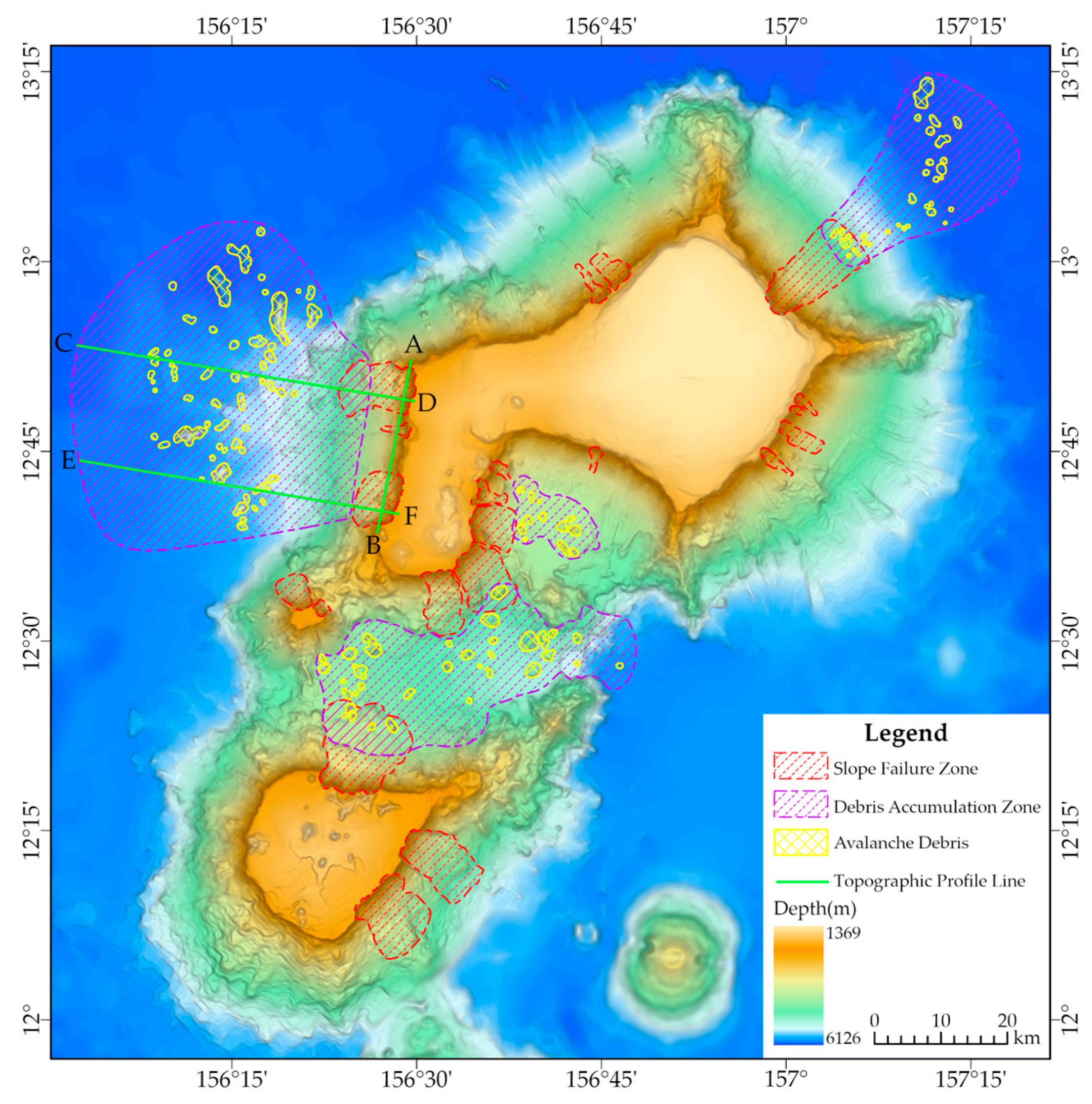
In this study, the failure characteristics of slopes were identified based on the topographic features of the Jiaxie Seamount Group. Based on the arc main scarp and sidewall characteristics, 21 failure zones were identified on the seamount slopes (Figure 3). Additionally, based on the characteristics of the avalanche debris and the accumulation patterns at the toe of the slopes, numerous avalanche debris and four debris accumulation zones were identified (Figure 4). The maximum zone of the avalanche debris measured about 13 km², and the maximum sliding distance was about 40 km. A typical debris aggregation phenomenon was observed at the toe of the slope within the Jiaxie Seamount Group. Due to the topography and geomorphology, some of the avalanche debris of the adjacent zones aggregated in the same area. The northern summit edge of the Weixie Guyot was characterized by a wavy, inward concavity, and the sliding surface exhibited a rough topography. Therefore, the presence of multiple slope failures was deemed possible. The area is situated at the intersection of the Weijia and Weixie Guyots, where the avalanche debris on both sides converges and exhibits signs of ongoing movement eastward. No apparent toe-of-slope bulge feature was present; however, there was a significant accumulation of debris.

Several slope failures were identified on the southwest flank of the Weijia Guyot, with avalanche debris clustered in distribution. To investigate the slope failure characteristics in this region, three topographic profiles were constructed at the AB, CD, and EF sites (Figure 4).

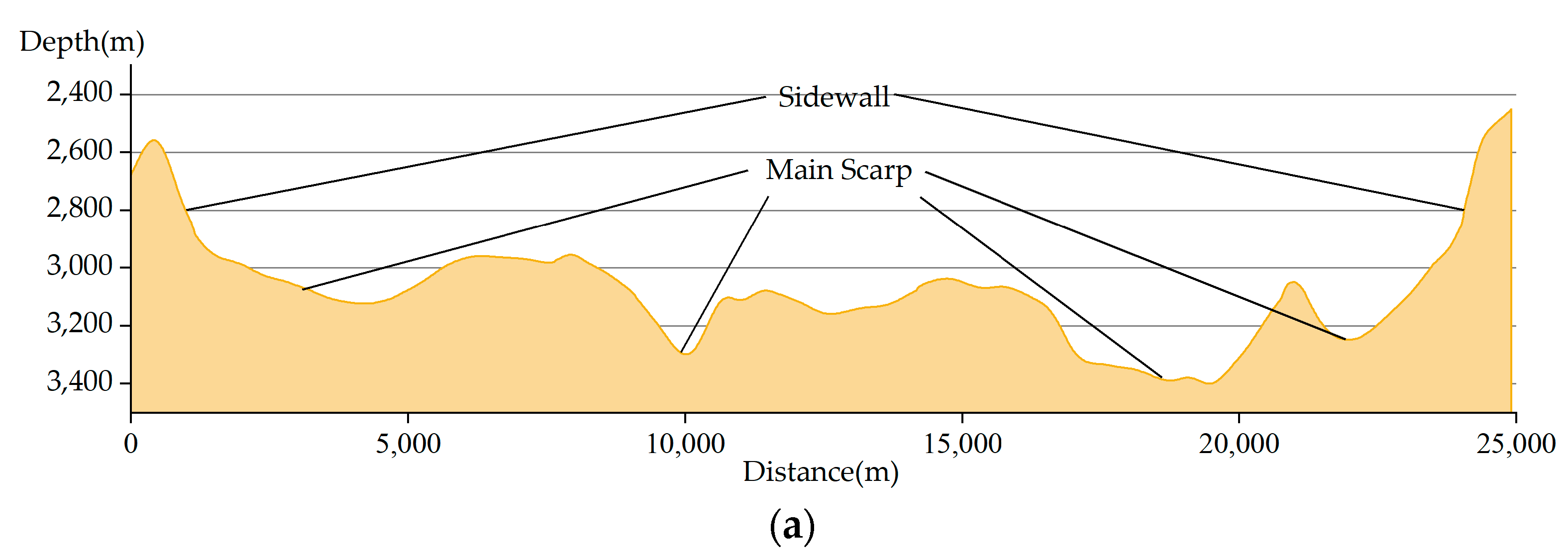
The topographic profile of the AB site is a transverse profile (Figure 5a), with a minimum water depth of about 2450 m, a maximum water depth of about 3399 m, and a maximum depth difference of about 949 m. In the figure, it is evident that the topography on both sides is steep, aligning with the sidewall characteristics of slope failure. There are four distinct arcuate concavities in the area, which align with the main scarp characteristics of slope failure. At a distance of around 12,500 m, there is a slight inward concavity. It is presumed that the slope failure at this site occurred earlier and was influenced by subsequent seawater erosion and adjacent slope failures, leading to the main scarp feature not being obvious. Thus, through topographic and geomorphological analyses, it was determined that there are several instances of slope failure in this area.

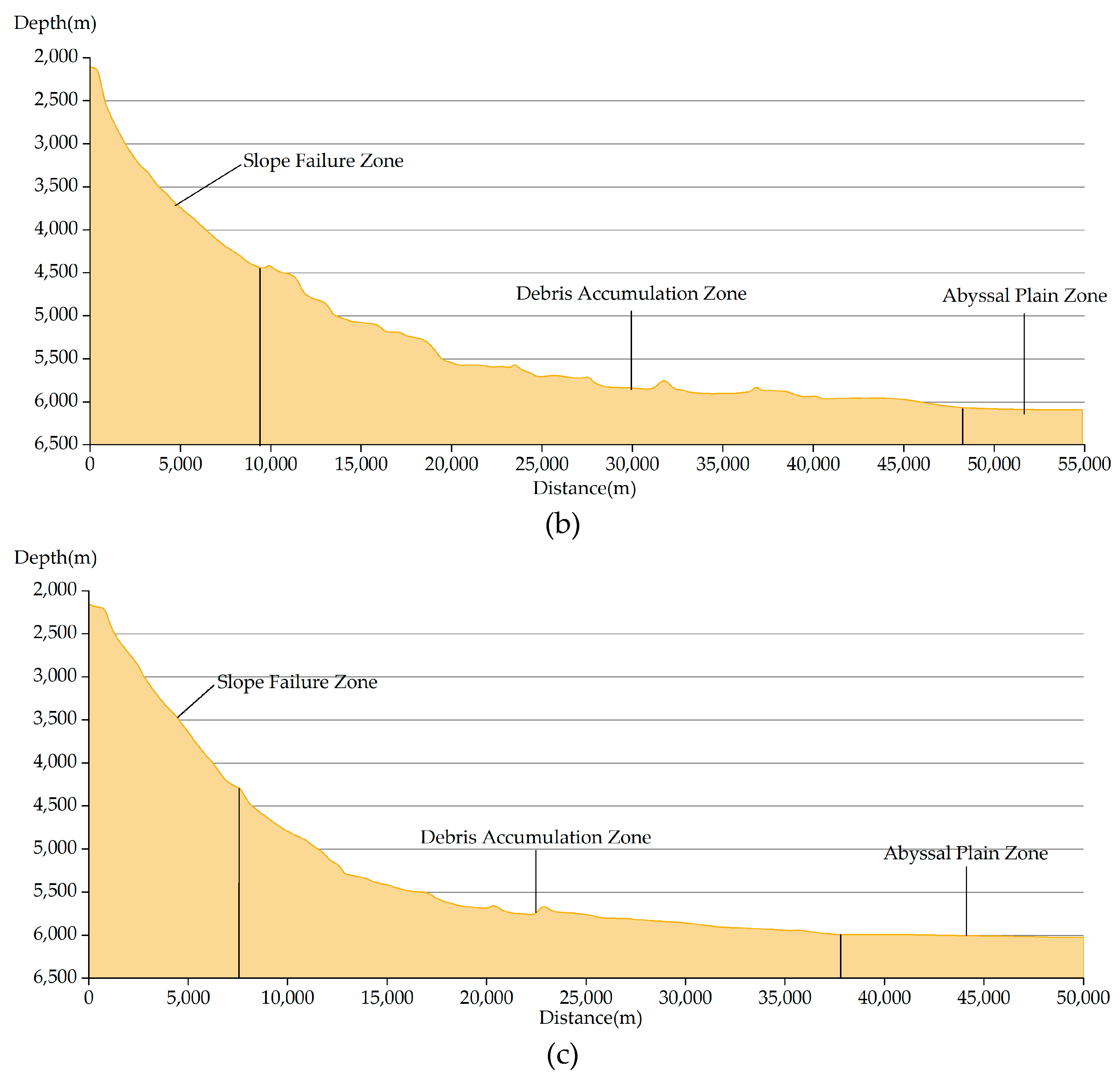
The topographic profile of the CD site is a longitudinal profile (Figure 5b), with a minimum water depth of about 2107 m, a maximum water depth of about 6094 m, and a maximum depth difference of about 3987 m. According to the longitudinal profile of the CD site, it can be divided into a slope failure zone, an avalanche debris accumulation zone, and an abyssal plain zone. About 10 km from the top of the main scarp is the slope failure zone, characterized by a steep, smooth terrain consistent with the main scarp feature. The debris accumulation zone is located 10 km to 48 km from the top of the main scarp. Due to the accumulation of a large amount of debris in this zone, it exhibits characteristics of a relatively gentle overall slope and rough terrain. Approximately 48 km from the summit of the main scarp, the region that extends backward is an abyssal plain zone characterized by a flat and smooth terrain, which aligns with the typical features of an abyssal plain.

The topographic profile of the EF site is a longitudinal profile (Figure 5c), featuring a minimum water depth of about 2154 m, a maximum water depth of about 6044 m, and a maximum depth variation of about 3890 m. According to the longitudinal profile of the EF site, it can be divided into a slope instability zone, a debris accumulation zone, and an abyssal plain zone. Approximately 7.5 km from the summit of the main scarp lies the slope failure area. Here, the terrain is steep and smooth, aligning with the main scarp terrain characteristics. The debris accumulation zone is situated 7.5 km to 38 km from the summit of the main scarp. In this area, the slope is gentler, the terrain is rugged, and only portions exhibit distinct raised features, suggesting that only a small amount of large debris has accumulated here. The region extending approximately 38 km from the main breakwater is the abyssal plain area, characterized by a flat terrain and a lack of significant undulations.

4.2. Analysis of the Independence of Assessment Indicators

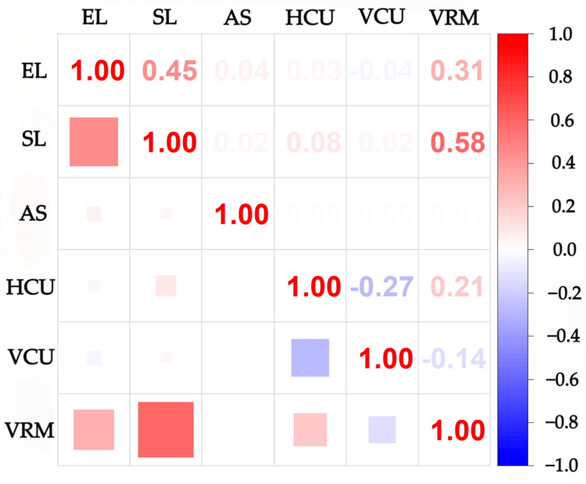
To assess the rationality of the selected assessment indicators, we calculated the correlations between six topographic factors of the Jiaxie Seamounts Group: water depth (EL), slope (SL), aspect (AS), planar curvature (HCU), profile curvature (VCU), and ruggedness (VRM). The aim was to confirm the independence of these influencing factors. The calculated Pearson’s correlation coefficient R indicates the correlation among the assessment indicators.

The results of the correlation calculations are shown in Figure 6. The absolute value of Pearson’s correlation coefficient R ranges from 0 to 0.1 for a very weak correlation, 0.1 to 0.4 for a weak correlation, 0.4 to 0.6 for a moderate correlation, 0.6 to 0.8 for a strong correlation, and 0.8 to 1.0 for a very strong correlation [44]. The correlation analysis results show that the degree of correlation among the assessment indicators varied from very weak to moderate. Among them, the correlation between slope and water depth and the ruggedness indicator VRM fell within the medium correlation range. The correlation between water depth and VRM, planar curvature and profile curvature and VRM, and profile curvature and VRM fell within the weak correlation range. The correlation among the remaining indicators fell within the very weak correlation range. Although there were some correlations between some of the assessment indicators, the definitions of these indicators indicate significant independence. Therefore, they can still be included in the assessment indicator system for seamount stability assessment.

4.3. Assessment of Seamount Stability

4.3.1. Weight of Evidence

To calculate the evidence weight, a failure dataset and an evidence factor dataset must first be established. The identified slope failure zones constituted the failure dataset, with 16 of these zones chosen as the training set and the remaining 5 zones used as the validation set. The evidence factor dataset was obtained by reclassifying the assessment indicators. The slope was reclassified into five categories: 0° to 2° (flat), 2° to 5° (a very gentle slope), 5° to 15° (a gentle slope), 15° to 25° (a steep slope), and over 25° (a very steep slope). The aspect was reclassified into eight categories: north, northeast, east, southeast, south, southwest, west, and northwest. The remaining assessment indicators were all reclassified into five categories based on the method of natural discontinuities, serving as evidence factors for the stability assessment (Figure 7).

By calculating the total number of pixels, the number of failure pixels, and the number of non-failure pixels within the assessment area using the training set, the a priori odds O(D) can be determined. The number of evidence factor pixels, the number of failure pixels within the evidence factor, and the number of non-failure pixels within the evidence factor were counted separately for each assessment metric. Similarly, the number of failure pixels in the non-evidence factor and the number of non-failure pixels in the non-evidence factor were also counted. These counts were used to compute the positive weights ($W^{+}$), negative weights ($W^{-}$), relative coefficients (C), and evidential weights (W) for each evidence factor. The weight of evidence for the slope factor was also calculated, as shown in

Table 1. Calculation of evidence weights for slope assessment indicators.

The Evidence Factor of Slope	0~2°	2~5°	5~15°	15~25°	Above 25°
Total number of pixels in the assessment area	8,750,609
Number of failure pixels in the assessment area	249,854
Number of non-failure pixels in the assessment area	8,500,755
A priori probability (O(F))	0.02939
Number of evidence factor pixels	4,235,894	1,518,983	1,919,017	821,485	255,230
Number of failure pixels in the evidence factor	5209	19,941	120,661	68,876	35,167
Number of non-failure pixels in the evidence factor	4,230,685	1,499,042	1,798,356	752,609	220,063
Number of failure pixels in the non-evidence factor	244,645	229,913	129,193	180,978	214,687
Number of non-failure pixels in the non-evidence factor	4,270,070	7,001,713	6,702,399	7,748,146	8,280,692
Positive weights ($W^{+}$)	−3.17270	−0.79277	0.82539	1.13580	1.69323
Negative weights ($W^{-}$)	0.66746	0.11082	−0.42188	−0.22980	−0.12547
Relative coefficients (C)	−3.84016	−0.90359	1.24727	1.36560	1.81870
Comprehensive weight of evidence (W)	−3.83902	−0.90246	1.24840	1.36673	1.81983

.

4.3.2. Failure Probability

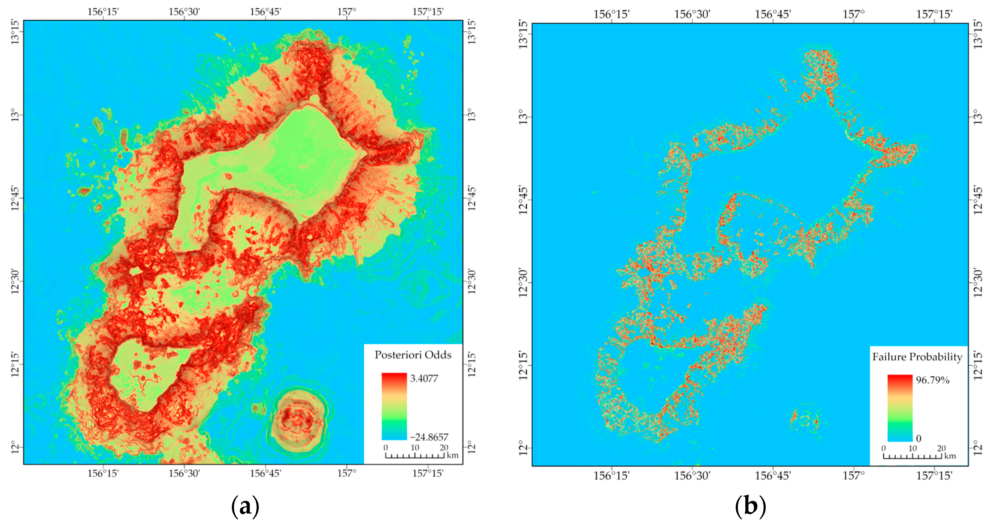
The calculated comprehensive weights of evidence are assigned to the pixels of each evidence factor, thereby obtaining the weight-of-evidence layer for each assessment indicator. Based on the calculated a priori odds and integration with the a posteriori odds formulas, the integrated a posteriori odds for each assessment indicator can be calculated. The entire a posteriori odds layer of all assessment indicators can be superimposed to obtain the entire a posteriori odds layer for the assessment area (Figure 8a). The calculated failure probability distributions are plotted based on Formula 17 for the total a posteriori probability (Figure 8b).

4.3.3. Stability Zoning Assessment

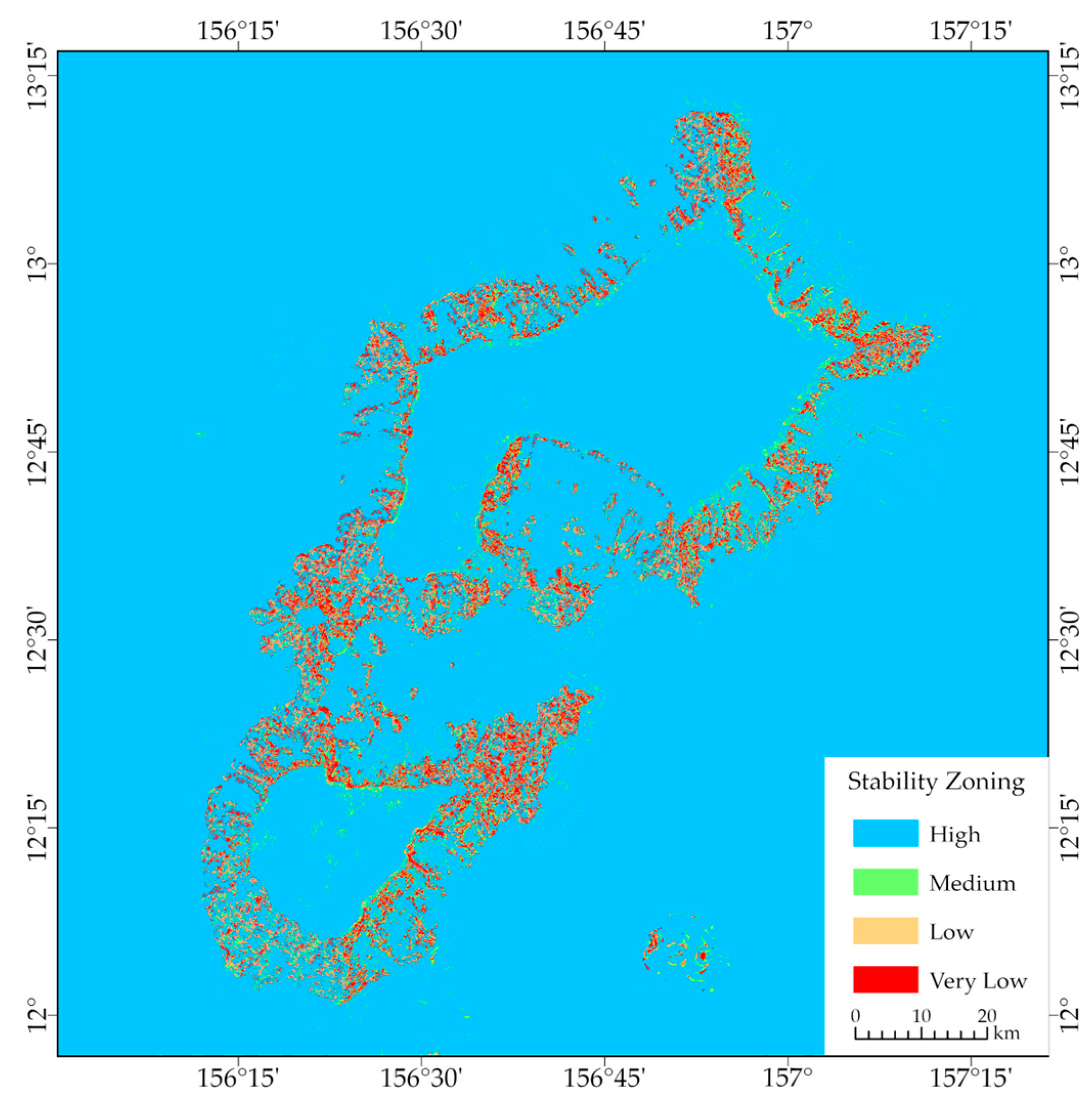
In the failure probability distribution map of the assessment area, it can be seen that the failure probability of the Jiaxie Seamount Group ranges from 0 to 96.79%. Considering the failure probability, intervals are classified as follows: less than 25% indicates a high-stability zone, 25% to 50% signifies a medium-stability zone, 50% to 75% corresponds to a low-stability zone, and over 75% denotes a very-low-stability zone. These four levels constitute the stability zoning assessment map of the Jiaxie Seamount Group (Figure 9).

In Figure 9, it is evident that, in the Jiaxie Seamount Group, high-stability zones are primarily located on the summit platform, the abyssal plain, and the smooth regions of the slope surface; low-stability and very-low-stability zones are predominantly found at the steep edges of the seamounts, in the upper parts of the ridges, and in the rugged areas; and medium-stability zones are mainly situated on the less steep slopes, indicating smoother areas. The detailed proportions of area under different stability levels and the proportions of failure area within each level are shown in

Table 2. Stability level grading and statistics on the area of each zone.

Probability Grading	Stability Level	Proportion of Zone Area	Proportion of Failure Area
Below 25%	High	93.04%	1.93%
25% to 50%	Medium	2.47%	10.50%
50% to 75%	Low	2.04%	13.89%
Above 75%	Very Low	2.45%	15.45%

.

The results of the stability assessment indicate that 93.04% of the assessed area is within the high-stability zone, 2.47% is in the medium-stability zone, 2.04% is in the low-stability zone, and 2.45% is in the very-low-stability zone. The failure area percentages are as follows: 1.93% within the high-stability zone, 10.50% within the medium-stability zone, 13.89% within the low-stability zone, and 15.45% within the very-low-stability zone. It is evident from the stability assessment of the topographic factors that the majority of the Jiaxie Seamount Group falls within the high-stability zone, with the combined area of the low-stability and very-low-stability zones constituting less than 4%. The proportion of failure areas gradually increases as stability diminishes.

4.4. WoE Model Validation

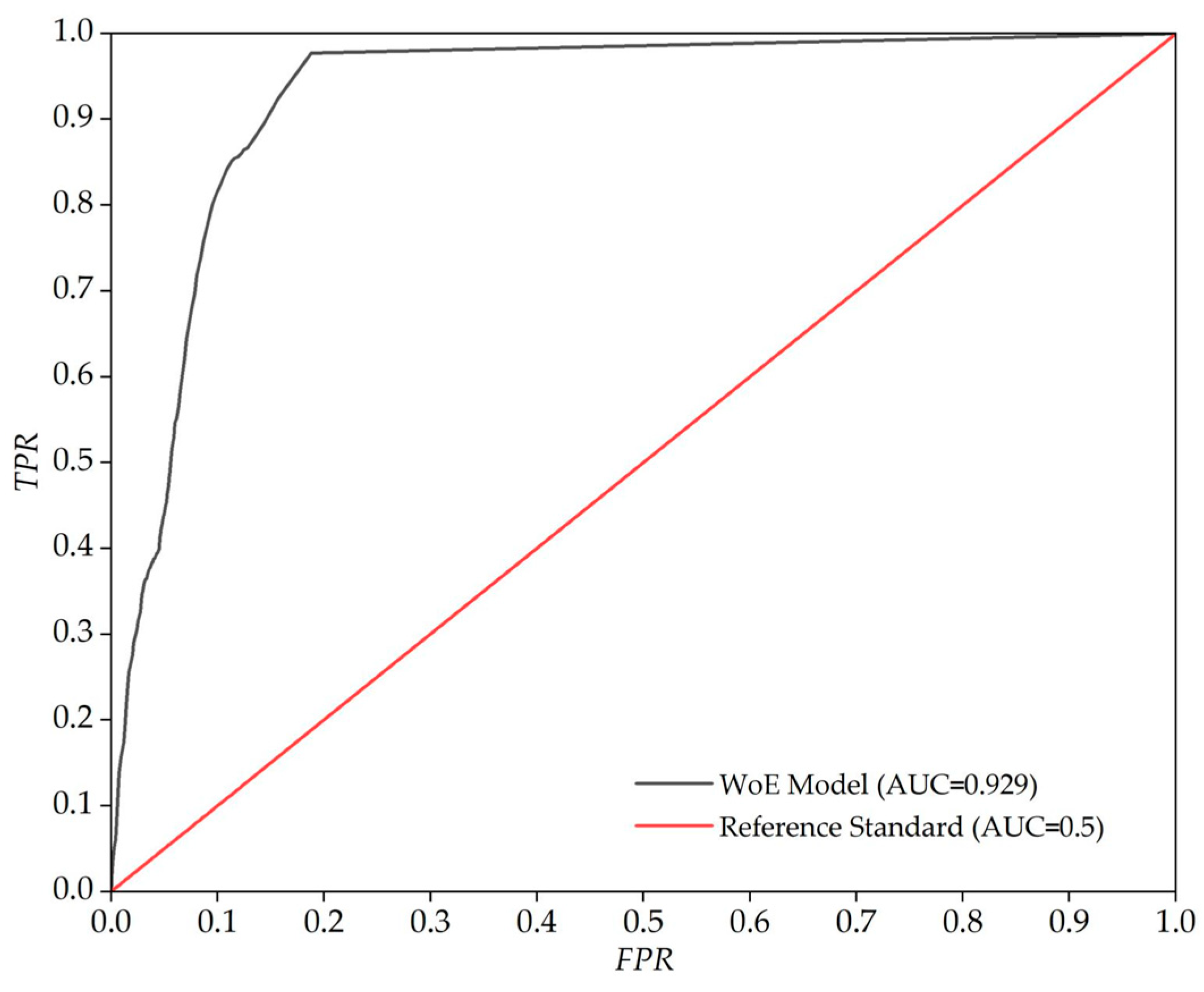
In this study, an ROC curve was used to assess the outcomes of the stability zoning assessment for the Jiaxie Seamount Group. The failure probability interval, ranging from 0 to 97%, was divided into 97 thresholds at 1% intervals. Subsequently, the true-positive rate (TPR) and false-positive rate (FPR) were computed for each of these thresholds. Some of the thresholds were selected, and their sample sizes and the TPR and FPR calculation results are shown in

Table 3. Validation sample size and calculations for TPR and FPR under partial thresholds.

Probability	TP	P	FP	N	TPR	FPR
96%	0	10,887	106	8,739,722	0.00000	0.00001
90%	560	10,887	26,488	8,739,722	0.05144	0.00303
80%	2776	10,887	144,179	8,739,722	0.25498	0.01650
70%	3813	10,887	260,892	8,739,722	0.35023	0.02985
60%	4178	10,887	339,595	8,739,722	0.38376	0.03886
50%	4328	10,887	388,274	8,739,722	0.39754	0.04443
40%	4785	10,887	435,879	8,739,722	0.43952	0.04987
30%	5945	10,887	524,392	8,739,722	0.54606	0.06000
20%	7819	10,887	703,906	8,739,722	0.71820	0.08054
10%	9256	10,887	985,202	8,739,722	0.85019	0.11273
0%	10,887	10,887	8,739,722	8,739,722	1.00000	1.00000

. By employing these metrics, an ROC curve was constructed, and the AUC value was determined (Figure 10). The AUC value of the WoE model was 0.929, indicating that the weight-of-evidence method has a high discriminative ability and applicability in evaluating seamount stability.

5. Conclusions

In this study, we assessed the stability of the Jiaxie Seamount Group in the western Pacific Ocean using the weight-of-evidence method. We constructed a seamount stability assessment model by analyzing the correlation between topographic factors and failure phenomena and verified its validity. The main conclusions of this study include the following:

(1)

There are obvious slope failure features in the Jiaxie Seamount Group, and typical slope failure zones, avalanche debris, and debris accumulation zones can be identified based on topographic features. Slope failure phenomena are distributed at the summit margins of three guyots: the Weijia, Weizhen, and Weixie Guyots. Among these, failure phenomena occur more frequently at the Weijia Guyot, which is the largest in size;

(2)

The six chosen topographic elements—water depth, slope, aspect, planar curvature, profile curvature, and VRM—demonstrate distinct independence and are appropriate for use as assessment indicators in evaluating the stability of seamounts;

(3)

The results of the stability zoning assessment for the Jiaxie Seamount Group indicate that the majority of the area falls within the high-stability zone, with less than 4% classified as low-stability and very-low-stability zones. High-stability zones are primarily located on summit platforms, deep-sea plains, and smooth slope surfaces; medium-stability zones are primarily located on relatively smooth steep slopes; and low-stability and very-low-stability zones are predominantly found on the steep edges of the guyots, on the upper ridges, and in areas with high ruggedness;

(4)

The results of the stability assessment of the Jiaxie Seamount Group were validated through an ROC curve. The calculated AUC value was 0.929, indicating that the weight-of-evidence method has a high discriminative ability and applicability in evaluating seamount stability.

In this study, the weight-of-evidence method was used to assess the stability of deep-sea seamounts, representing a preliminary exploration into the stability of the deep seabed. It offers scientific support for deep-sea resource extraction and engineering construction. Nevertheless, it is subject to the following limitations:

(1)

Due to the difficulty in obtaining deep-sea environmental data, only seafloor topographic data were used for the stability assessment in this study, which may have resulted in a somewhat one-sided assessment;

(2)

The weight-of-evidence approach requires the use of a slope failure dataset; however, no deep-sea slope failure databases are available. The dataset used in this study was compiled through a visual analysis of seafloor topography, which means that the data may be subjective.

References

1. Jiang, X.; Dong, C.; Ji, Y.; Wang, C.; Shu, Y.; Liu, L.; Ji, J. Influences of Deep-Water Seamounts on the Hydrodynamic Environment in the Northwestern Pacific Ocean. J. Geophys. Res. Ocean. 2021, 126, e2021JC017396. [Google Scholar] [CrossRef]
2. Wang, X.; Li, H.; Zhang, J.; Chen, J.; Xie, X.; Xie, W.; Yin, K.; Zhang, D.; Diana, R.; Kao, S.-J. Seamounts Generate Efficient Active Transport Loops to Nourish the Twilight Ecosystem. Sci. Adv. 2024, 10, eadk6833. [Google Scholar] [CrossRef]
3. Samadi, S.; Bottan, L.; Macpherson, E.; Forges, B.; Boisselier, M.-C. Seamount Endemism Questioned by the Geographic Distribution and Population Genetic Structure of Marine Invertebrates. Mar. Biol. 2006, 149, 1463–1475. [Google Scholar] [CrossRef]
4. Morato, T.; Varkey, D.A.; Damaso, C.; Machete, M.; Santos, M.; Prieto, R.; Santos, R.S.; Pitcher, T.J. Evidence of a Seamount Effect on Aggregating Visitors. Mar. Ecol. Prog. Ser. 2008, 357, 23–32. [Google Scholar] [CrossRef]
5. Morato, T.; Hoyle, S.D.; Allain, V.; Nicol, S.J. Seamounts Are Hotspots of Pelagic Biodiversity in the Open Ocean. Proc. Natl. Acad. Sci. USA 2010, 107, 9707–9711. [Google Scholar] [CrossRef]
6. Hein, J.; Mizell, K.; Koschinsky, A.; Conrad, T. Deep-Ocean Mineral Deposits as a Source of Critical Metals for High-and Green-Technology Applications: Comparison with Land-Based Resources. Ore Geol. Rev. 2012, 51, 1–14. [Google Scholar] [CrossRef]
7. Mizell, K.; Hein, J.R.; Au, M.; Gartman, A. Estimates of Metals Contained in Abyssal Manganese Nodules and Ferromanganese Crusts in the Global Ocean Based on Regional Variations and Genetic Types of Nodules. In Perspectives on Deep-Sea Mining: Sustainability, Technology, Environmental Policy and Management; Sharma, R., Ed.; Springer International Publishing: Cham, Switzerland, 2022; pp. 53–80. ISBN 978-3-030-87982-2. [Google Scholar]
8. Holzheid, A.; Zhao, H.; Cabus, T.; Fan, L.; Kuhn, T.; Sun, L.; Tao, C.; Haeckel, M.; Hoang, D.; Kelly, N.; et al. Deep-Sea Mining of Massive Sulfides: Balancing Impacts on Biodiversity and Ecosystem, Technological Challenges and Law of the Sea. Mar. Policy 2024, 167, 106289. [Google Scholar] [CrossRef]
9. Liu, X.; Li, H.; Zhou, T.; Xu, C. Multibeam Seafloor Topography-Geomorphology Integrated Detection Technology. In Proceedings of the 2011 International Conference on Multimedia Technology, Hangzhou, China, 26–28 July 2011; pp. 3575–3578. [Google Scholar]
10. Kumar, D.; Krishnan, A.; Kuttikrishnan, G.; Ramadass, G.A. Air-Lift Pump Systems for Vertical Solid Particle Transport: A Comprehensive Review and Deep Sea Mining Potential. Ocean. Eng. 2024, 297, 116928. [Google Scholar] [CrossRef]
11. Nian, T.; Liu, B.; Yin, P. Seafloor Slope Stability under Adverse Conditions Using Energy Approach. Appl. Mech. Mater. 2013, 405–408, 1445–1448. [Google Scholar] [CrossRef]
12. Wang, Y.; Wang, R.; Zhang, J.-M. Large-Scale Seismic Seafloor Stability Analysis in the South China Sea. Ocean. Eng. 2021, 135, 109334. [Google Scholar] [CrossRef]
13. Deplus, C.; Le Friant, A.; Boudon, G.; Komorowski, J.-C.; Villemant, B.; Harford, C.; Ségoufin, J.; Cheminée, J.-L. Submarine Evidence for Large-Scale Debris Avalanches in the Lesser Antilles Arc. Earth Planet. Sci. Lett. 2001, 192, 145–157. [Google Scholar] [CrossRef]
14. Saint-Ange, F.; Bachèlery, P.; Babonneau, N.; Michon, L.; Jorry, S.J. Volcaniclastic Sedimentation on the Submarine Slopes of a Basaltic Hotspot Volcano: Piton de La Fournaise Volcano (La Réunion Island, Indian Ocean). Mar. Geol. 2013, 337, 35–52. [Google Scholar] [CrossRef]
15. Chang, Y.-C.; Mitchell, N.C.; Quartau, R. Landslides in the Upper Submarine Slopes of Volcanic Islands: The Central Azores. Geochem. Geophys. Geosyst. 2021, 22, e2021GC009833. [Google Scholar] [CrossRef]
16. Acharya, G.; De Smedt, F.; Long, N.T. Assessing Landslide Hazard in GIS: A Case Study from Rasuwa, Nepal. Bull. Eng. Geol. Environ. 2006, 65, 99–107. [Google Scholar] [CrossRef]
17. Ciabatta, L.; Camici, S.; Brocca, L.; Ponziani, F.; Stelluti, M.; Berni, N.; Moramarco, T. Assessing the Impact of Climate-Change Scenarios on Landslide Occurrence in Umbria Region, Italy. J. Hydrol. 2016, 541, 285–295. [Google Scholar] [CrossRef]
18. Lin, Q.; Steger, S.; Pittore, M.; Zhang, J.; Wang, L.; Jiang, T.; Wang, Y. Evaluation of Potential Changes in Landslide Susceptibility and Landslide Occurrence Frequency in China under Climate Change. Sci. Total Environ. 2022, 850, 158049. [Google Scholar] [CrossRef]
19. Song, Y.; Na, W.; Jun, C.; Kim, S.Y. Comparative Analysis of Slope Stability Factors and a Hydrological Dataset for Landslide Assessment. Nat. Hazards 2025, 121, 3981–3996. [Google Scholar] [CrossRef]
20. Vikara, D.; Remson, D.; Khanna, V. Machine Learning-Informed Ensemble Framework for Evaluating Shale Gas Production Potential: Case Study in the Marcellus Shale. J. Nat. Gas Sci. Eng. 2020, 84, 103679. [Google Scholar] [CrossRef]
21. Wang, H.; Zhang, L.; Luo, H.; He, J.; Cheung, R.W.M. AI-Powered Landslide Susceptibility Assessment in Hong Kong. Eng. Geol. 2021, 288, 106103. [Google Scholar] [CrossRef]
22. Tan, L.; Zhou, M.; Wang, F. A Probabilistic Assessment Framework for Submarine Landslide Susceptibility in Continental Slopes with Rich Gas Hydrates. J. Mar. Sci. Eng. 2023, 11, 1366. [Google Scholar] [CrossRef]
23. Wei, X.; Gardoni, P.; Zhang, L.; Tan, L.; Liu, D.; Du, C.; Li, H. Improving Pixel-Based Regional Landslide Susceptibility Mapping. Geosci. Front. 2024, 15, 101782. [Google Scholar] [CrossRef]
24. Dondin, F.J.-Y.; Heap, M.J.; Robertson, R.E.A.; Dorville, J.-F.M.; Carey, S. Flank Instability Assessment at Kick-’em-Jenny Submarine Volcano (Grenada, Lesser Antilles): A Multidisciplinary Approach Using Experiments and Modeling. Bull. Volcanol. 2016, 79, 5. [Google Scholar] [CrossRef]
25. Govorov, I.N.; Gerasimov, N.S.; Simanenko, V.P. Rubidium-Strontium Isochron of Ankaramite-Trachybasalt Assotiation of the Marcus-Wake Rise (Pacific). Dokl. Akad. Nauk. 1996, 347, 780–783. [Google Scholar]
26. Mel’nikov, M.E.; Tugolesov, D.D.; Pletnev, S.P. The Structure of the Incoherent Sediments in the Ita Mai Tai Guyot (Pacific Ocean) Based on Geoacoustic Profiling Data. Oceanology 2010, 50, 582–590. [Google Scholar] [CrossRef]
27. Pletnev, S.P. Main Types of Aptian–Cenomanian Sedimentary Rocks on Guyots of the Magellan Mountains, Pacific Ocean. Russ. J. Pac. Geol. 2019, 13, 436–445. [Google Scholar] [CrossRef]
28. Bulmer, M.H.; Wilson, J.B. Comparison of Flat-Topped Stellate Seamounts on Earth’s Seafloor with Stellate Domes on Venus Using Side-Scan Sonar and Magellan Synthetic Aperture Radar. Earth Planet. Sci. Lett. 1999, 171, 277–287. [Google Scholar] [CrossRef]
29. Wang, X.; Li, H.; Cheng, Y.; Yao, P.; Chu, F.; Ma, W.; Wang, H.; Lv, S.; Li, X.; Li, Z.; et al. Submarine Morphological Description of the Ancient Archipelagic Aprons in the Marcus–Wake Seamount Group, Northwestern Pacific Ocean. J. Mar. Sci. Eng. 2024, 12, 670. [Google Scholar] [CrossRef]
30. Becker, J.J.; Sandwell, D.T.; Smith, W.H.F.; Braud, J.; Binder, B.; Depner, J.; Fabre, D.; Factor, J.; Ingalls, S.; Kim, S.-H.; et al. Global Bathymetry and Elevation Data at 30 Arc Seconds Resolution: SRTM30_PLUS. Mar. Geod. 2009, 32, 355–371. [Google Scholar] [CrossRef]
31. Bird, P. An Updated Digital Model of Plate Boundaries. Geochem. Geophys. Geosyst. 2003, 4, 1027. [Google Scholar] [CrossRef]
32. Wlodarczyk-Sielicka, M.; Blaszczak-Bak, W. Processing of Bathymetric Data: The Fusion of New Reduction Methods for Spatial Big Data. Sensors 2020, 20, 6207. [Google Scholar] [CrossRef]
33. Zhao, J.; Yan, J.; Zhang, H.; Zhang, Y.; Wang, A. A New Method for Weakening the Combined Effect of Residual Errors on Multibeam Bathymetric Data. Mar. Geophys. Res. 2014, 35, 379–394. [Google Scholar] [CrossRef]
34. Masson, D.G.; Watts, A.B.; Gee, M.J.R.; Urgeles, R.; Mitchell, N.C.; Le Bas, T.P.; Canals, M. Slope Failures on the Flanks of the Western Canary Islands. Earth-Sci. Rev. 2002, 57, 1–35. [Google Scholar] [CrossRef]
35. Watt, S.F.L.; Talling, P.J.; Hunt, J.E. New Insights into the Emplacement Dynamics of Volcanic Island Landslides. Oceanography 2015, 27, 46–57. [Google Scholar] [CrossRef]
36. Berné, S.; Vagner, P.; Guichard, F.; Lericolais, G.; Liu, Z.; Trentesaux, A.; Yin, P.; Yi, H.I. Pleistocene Forced Regressions and Tidal Sand Ridges in the East China Sea. Mar. Geol. 2002, 188, 293–315. [Google Scholar] [CrossRef]
37. Canals, M.; Lastras, G.; Urgeles, R.; Casamor, J.L.; Mienert, J.; Cattaneo, A.; De Batist, M.; Haflidason, H.; Imbo, Y.; Laberg, J.S.; et al. Slope Failure Dynamics and Impacts from Seafloor and Shallow Sub-Seafloor Geophysical Data: Case Studies from the COSTA Project. Mar. Geol. 2004, 213, 9–72. [Google Scholar] [CrossRef]
38. Green, A.; Uken, R. Submarine Landsliding and Canyon Evolution on the Northern KwaZulu-Natal Continental Shelf, South Africa, SW Indian Ocean. Mar. Geol. 2008, 254, 152–170. [Google Scholar] [CrossRef]
39. Weed, D.L. Weight of Evidence: A Review of Concept and Methods. Risk Anal. 2005, 25, 1545–1557. [Google Scholar] [CrossRef]
40. Hardy, A.; Benford, D.; Halldorsson, T.; Jeger, M.J.; Knutsen, H.K.; More, S.; Naegeli, H.; Noteborn, H.; Ockleford, C.; Ricci, A.; et al. Guidance on the Use of the Weight of Evidence Approach in Scientific Assessments. EFSA J. 2017, 15, e04971. [Google Scholar] [CrossRef]
41. Velmurugan, J.; Venkatesan, M. Soft Prediction Model for Spatial Data Analysis. Int. J. Glob. Environ. Issues 2018, 17, 130–143. [Google Scholar] [CrossRef]
42. Fawcett, T. An Introduction to ROC Analysis. Pattern Recognit. Lett. 2006, 27, 861–874. [Google Scholar] [CrossRef]
43. Hand, D.J. Measuring Classifier Performance: A Coherent Alternative to the Area under the ROC Curve. Mach. Learn. 2009, 77, 103–123. [Google Scholar] [CrossRef]
44. Kader, G.; Franklin, C. The Evolution of Pearson’s Correlation Coefficient. Math. Teach. 2008, 102, 292–299. [Google Scholar] [CrossRef]
Figure 1. Bathymetric map of the Magellan Seamount Group. Blue boxes highlight the study area. Bathymetry data are from GEBCO [30]. Jagged blue lines mark the plate boundaries. Plate boundary data are from PB2002 [31]. The white-shaded zone indicates the extent of the Magellan Seamount Group.
Jmse 13 01001 g001
Figure 2. Map depicting the VRM calculation results. The curved red strip is typically positioned at the top of the main scarp.
Jmse 13 01001 g002
Figure 3. Extracted assessment indicators: (a) water depth, (b) slope, (c) aspect, (d) planar curvature, (e) profile curvature, and (f) VRM.
Jmse 13 01001 g003
Figure 4. Map of identification results of slope failure. Red denotes slope failure zones, purple denotes debris accumulation zones, yellow denotes avalanche debris, and green denotes the topographic profile location.
Jmse 13 01001 g004
Figure 5. Topographic profile of the southwestern flank of the Weijia Guyot: (a) the topographic profile of the AB site, (b) the topographic profile of the CD site, and (c) the topographic profile of the EF site.
Jmse 13 01001 g005aJmse 13 01001 g005b
Figure 6. Hotspot map of correlation between assessment indicators. Red indicates higher positive correlations, blue indicates higher negative correlations, and lighter colors indicate lower correlations.
Jmse 13 01001 g006
Figure 7. The evidence factor dataset: a total of 33 evidence factors were delineated based on six terrain assessment indicators.
Jmse 13 01001 g007
Figure 8. (a) The comprehensive posteriori odds layer for the assessment area; (b) the calculated failure probability distributions.
Jmse 13 01001 g008
Figure 9. Stability zoning assessment map of the Jiaxie Seamount Group. Red indicates the very-low-stability zone, orange indicates the low-stability zone, green indicates the medium-stability zone, and blue indicates the high-stability zone.
Jmse 13 01001 g009
Figure 10. ROC curves were plotted using the FPR and TPR based on the WoE model. The horizontal axis represents the FPR, the vertical axis represents the TPR, the red line signifies the reference standard line, and the gray line denotes the WoE model’s ROC curve.
Jmse 13 01001 g010