A Three-Dimensional Routing Protocol for Underwater Acoustic Sensor Networks Based on Fuzzy Logic Reasoning

Abstract

Underwater acoustic sensor networks (UASNs) play an increasingly crucial role in both civilian and military fields. However, existing routing protocols primarily rely on node position information for forwarding decisions, neglecting link quality and energy efficiency. To address these limitations, we propose a fuzzy logic reasoning adaptive forwarding (FLRAF) routing protocol for three-dimensional (3D) UASNs. First, the FLRAF method redefines a conical forwarding region to prioritize nodes with greater effective advance distance, thereby reducing path deviations and minimizing the total number of hops. Unlike traditional approaches based on pipeline or hemispherical forwarding regions, this design ensures directional consistency in multihop forwarding, which improves transmission efficiency and energy utilization. Second, we design a nested fuzzy inference system for forwarding node selection. The inner inference system evaluates link quality by integrating the signal-to-noise ratio and some metrics related to the packet reception rate. This approach enhances robustness against transient fluctuations and provides a more stable estimation of link quality trends in dynamic underwater environments. The outer inference system incorporates link quality index, residual energy, and effective advance distance to rank candidate nodes. This multimetric decision model achieves a balanced trade-off between transmission reliability and energy efficiency. Simulation results confirm that the FLRAF method outperforms existing protocols under varying node densities and mobility conditions. It achieves a higher packet delivery rate, extended network lifetime, and lower energy consumption. These results demonstrate that the FLRAF method effectively addresses the challenges of energy constraints and unreliable links in 3D UASNs, making it a promising solution for adaptive and energy-efficient underwater communication.

1. Introduction

The Internet of Things (IoT) seeks to connect all aspects of our world through a unified infrastructure, enabling us to control and monitor their status anytime. IoT research has made great progress in the commercial and industrial fields [1,2,3], enhancing the potential for its application in underwater environments. Consequently, research on the Internet of Underwater Things (IoUT) is increasingly capturing the interest of researchers [4,5].

IoUT technology plays a crucial role in military defense, smart coasts and oceans, underwater detection, disaster prediction, and other civilian and military fields [6,7,8]. The most important branch of IoUT research is underwater acoustic sensor networks (UASNs). The construction of UASNs for data collection has gradually become an effective ocean exploration method [9]. In terrestrial sensor networks, electromagnetic waves are undoubtedly an efficient medium for wireless transmission. However, in underwater environments, electromagnetic waves suffer from severe attenuation, which makes long-distance propagation challenging. In addition, although light waves can propagate underwater, they are significantly affected by scattering and absorption, resulting in very short transmission distances. Therefore, acoustic waves hold distinct advantages in underwater communication as they can penetrate water layers and transmit over longer distances.

However, there are also many drawbacks, such as high transmission losses, multipath effects, limited bandwidth, long delays, and Doppler propagation, which pose huge challenges in conducting relevant research [10]. In addition, underwater nodes are affected by movement caused by water currents and tides, causing the network topology to change continuously, which complicates network management and communication. The accurate locations of underwater nodes are particularly difficult to obtain since Global Positioning System (GPS) signals cannot propagate underwater. Additionally, since underwater nodes are typically battery-powered, managing energy consumption effectively to prolong the network lifetime is a key challenge. These problems make it impossible to apply terrestrial wireless sensor network technology directly to an underwater environment, so it is urgent to design an energy-efficient, scalable, and adaptive underwater acoustic routing protocol.

To address these challenges, various routing protocols have been proposed for UASNs. The main objective of the first category of routing protocols is to improve the energy efficiency of sensor nodes, which in turn helps to prolong the lifespan of the entire network. In [11], the authors applied an offline centralized algorithm to transform the energy consumption balance challenge into an optimal data distribution problem. A flaw in the study is that the forwarding node is frequently selected. In [12], the authors used machine learning technology, Q-learning (QL), to solve the problem mentioned above. The selection of the forwarding node is determined by its remaining energy and the group energy of its neighboring nodes. The phenomenon of routing voids in the protocol is also avoided. In addition, ref. [13] proposed a new baseline lightweight energy-aware opportunistic routing (EnOR) protocol. EnOR employs timer-based coordination to set candidate forwarding priorities, enabling efficient time slot assignment. The way the protocol calculates the priority is just a simple algebraic operation. However, the input parameters, such as the residual energy, are often uncertain and fuzzy, which cannot be described and dealt with by a pure algebraic operation.

Another branch called cluster-based routing protocols was first proposed in [14], in which whether a node is selected as a cluster head (CH) node is determined by the number of CHs required and how many times the node has been CH before. Compared to [14], ref. [15] provided a more detailed method for selecting the CH node with minimal energy consumption and data traffic load. Additionally, the forwarding node can dynamically adjust its transmission power and prevent repeated selection of the same CH node. Ref. [16] reduced the impact of acoustic interference on data transmission by limiting the Time Division Multiple Access (TDMA) scheduling of parallel data transmission and establishes an efficient and reliable intra-cluster hierarchical route for data transmission.

However, these protocols typically focus on balancing energy consumption, which may result in a low packet transmission success rate. In addition, additional network coordination may be required, such as frequent node selection or CH election. These processes can bring additional latency, which affects the need for real-time data transmission.

The second category of the routing protocol prioritizes the reliability of data transmission. In [17], the protocol uses the Dijkstra algorithm to select forwarding nodes with the least neighbors to avoid collision. In [18], the directional flooding-based routing (DFR) protocol relies on packet flooding technology to improve reliability, controlling the number of nodes that flood packets and determining the number of nodes that forward them based on link quality. However, when the DFR protocol is running, the network configuration parameters are fixed, which makes it unable to deal with system changes. Consequently, the intelligent directional flooding routing (iDFR) protocol was introduced in [19], along with two new DFR versions to dynamically reflect the quality of service (QoS). The flooding area can be dynamically adjusted according to the QoS feedback provided by the sink in these protocols.

These protocols prioritize the integrity of data transmission and often do not adequately consider the balance of energy consumption. For example, the DFR protocol ensures the reliability of data transmission by increasing the number of nodes participating in forwarding. However, this method increases energy consumption, particularly in densely networked scenarios. This flooding strategy may cause excessive redundant data transmissions.

The first branch of the last type of routing protocol is the depth-based routing protocol, which requires only depth information. Ref. [20] introduced a depth-based routing (DBR) protocol, where the most suitable forwarding node is selected based on the maximum depth difference. Building on the work in [20], ref. [21] introduced a more lightweight depth-based routing protocol (LDBR) that considers node energy. When a node has a shallower depth and higher energy, it is more likely to participate in the routing process. In [22], the authors proposed the reliable and stability-aware routing (RSAR) protocol, aimed at reducing packet loss and improving energy efficiency. The RSAR protocol introduces a novel approach by categorizing the network into five energy levels from top to bottom, selecting the optimal forwarding node based on depth information, residual energy, and energy level. Furthermore, ref. [23] introduced a parameter called the depth threshold into the routing process and increases the consideration of the number of transmission hops, thereby ensuring the successful transmission of packets.

Another branch is the location-based routing protocol. In [24], a vector-based forwarding (VBF) routing protocol was proposed, where packets are forwarded through the constructed virtual pipeline. However, the constant radius of the pipeline greatly impacts the performance of VBF. On the other hand, VBF cannot cope with the routing void phenomenon effectively. To increase the robustness and scalability of the previous protocol, the authors in [25] proposed the hop-by-hop VBF (HH-VBF) protocol, where the direction of the routing pipeline dynamically changes based on node distribution. Additionally, to reduce the impact of routing voids, ref. [26] provided its solution. Furthermore, two studies have outlined the routing protocol design in two stages: the first involves defining the forwarding area, and the second selects a forwarding node from the candidate set using various methods. For instance, game theory can be used to design strategy sets and gain functions or to derive forwarding probability through the Nash equilibrium [27]. Alternatively, forwarding probability can be calculated directly from node location information [28]. However, neither of these studies considered energy management; therefore, the network lifetime cannot be guaranteed.

In addition to routing protocols, several studies have also provided valuable methodological inspiration and technical guidance for enhancing real-time adaptive routing and intelligent decision-making strategies in UASNs. For example, studies on high-precision localization using multisensor association in space environments [29], the real-time trajectory planning and tracking control of bionic underwater robots in dynamic environments [30], and the design of a forward-looking sonar system with a lightweight multiscale attention network for environmental perception and intelligent decision making [31] offer important references for developing UASN systems with improved environmental awareness and dynamic adaptability.

The research purpose of this paper is to optimize the forwarding process of the three-dimensional (3D) underwater acoustic sensor network (UASN) routing protocol by using a fuzzy reasoning system, and the most important part is to deduce the candidate priority of nodes. The fuzzy logic reasoning system has already made important contributions to the research of opportunistic networks and ad hoc networks [32,33]. Inspired by these developments, we design a fuzzy logic reasoning adaptive forwarding (FLRAF) routing protocol for 3D UASNs and select the forwarding nodes using the fuzzy logic reasoning tool. We innovatively build a nested fuzzy logic reasoning system to determine node candidate priorities. The inner layer obtains the link quality index ($LQI$), while the outer layer determines node candidate priorities. In the process of obtaining $LQI$, refs. [34,35] inspires us, but after obtaining the cumulative packet reception rate ($PRR$), a series of $PRR$ values are used for calculating its coefficient of variation to serve as one of the fuzzy input variables, which may lead to a misjudgment of the link quality, because when the network encounters an outlier due to a brief emergency, the use of the coefficient of variation will have a significant impact on the fuzzy output. Therefore, we innovatively use the interquartile range of the cumulative $PRR$ value as one of the inputs of the link quality assessment task to evaluate the $LQI$ more comprehensively. Finally, we highlight the key innovations of the proposed FLRAF method.

(1)

The FLRAF routing protocol redefines the geometric boundary and selection criteria of the new forwarding area. It allows more suitable nodes to participate in the forwarding process and prevents unnecessary forwarding by nodes in unfavorable positions, thus reducing transmission redundancy. In addition, unlike traditional approaches based on pipeline or hemispherical forwarding regions, the conical forwarding area helps maintain the directional consistency of multihop forwarding paths from the source node, minimizing path deviations and thereby reducing the total number of hops required for transmission, which improves forwarding efficiency and ensures higher energy efficiency.

(2)

The FLRAF routing protocol designs a fuzzy logic reasoning system to improve the accuracy of link quality assessment. The system comprehensively analyzes the smoothed $PRR$ obtained through exponentially weighted moving average processing ($EWMA\_SPRR$), the signal-to-noise ratio ($SNR$), and the interquartile range ($IQR$) of the $PRR$ to complete the $LQI$ assessment task. By incorporating $IQR$ and $EWMA\_SPRR$ into link quality assessment, the proposed method improves robustness against transient fluctuations and provides a more stable estimation of link quality trends, ensuring accurate and reliable evaluation in dynamic underwater environments.

(3)

The FLRAF routing protocol builds a nested fuzzy logic reasoning system to complete the selection of candidate sets in the forwarding region. The inner inference system obtains the $LQI$ between nodes, while the outer inference system comprehensively considers the output of inner inference, the residual energy ($RE$), and the effective advance distance ($AD$) of nodes to obtain the priority ranking. By incorporating a novel multimetric fuzzy logic decision model, the method improves the packet delivery rate of the network and some parameters related to energy consumption.

The rest of this article is structured as follows. Section 2 presents the detailed implementation of the FLRAF protocol, including its forwarding process and fuzzy-logic-based decision strategy. Section 3 provides a comprehensive performance comparison with existing routing protocols under various simulation scenarios. Section 4 summarizes the main findings, discusses current research limitations, and outlines future work directions to enhance the adaptability and intelligence of underwater routing protocols.

2. Description of the Proposed Approach

2.1. Network Architecture

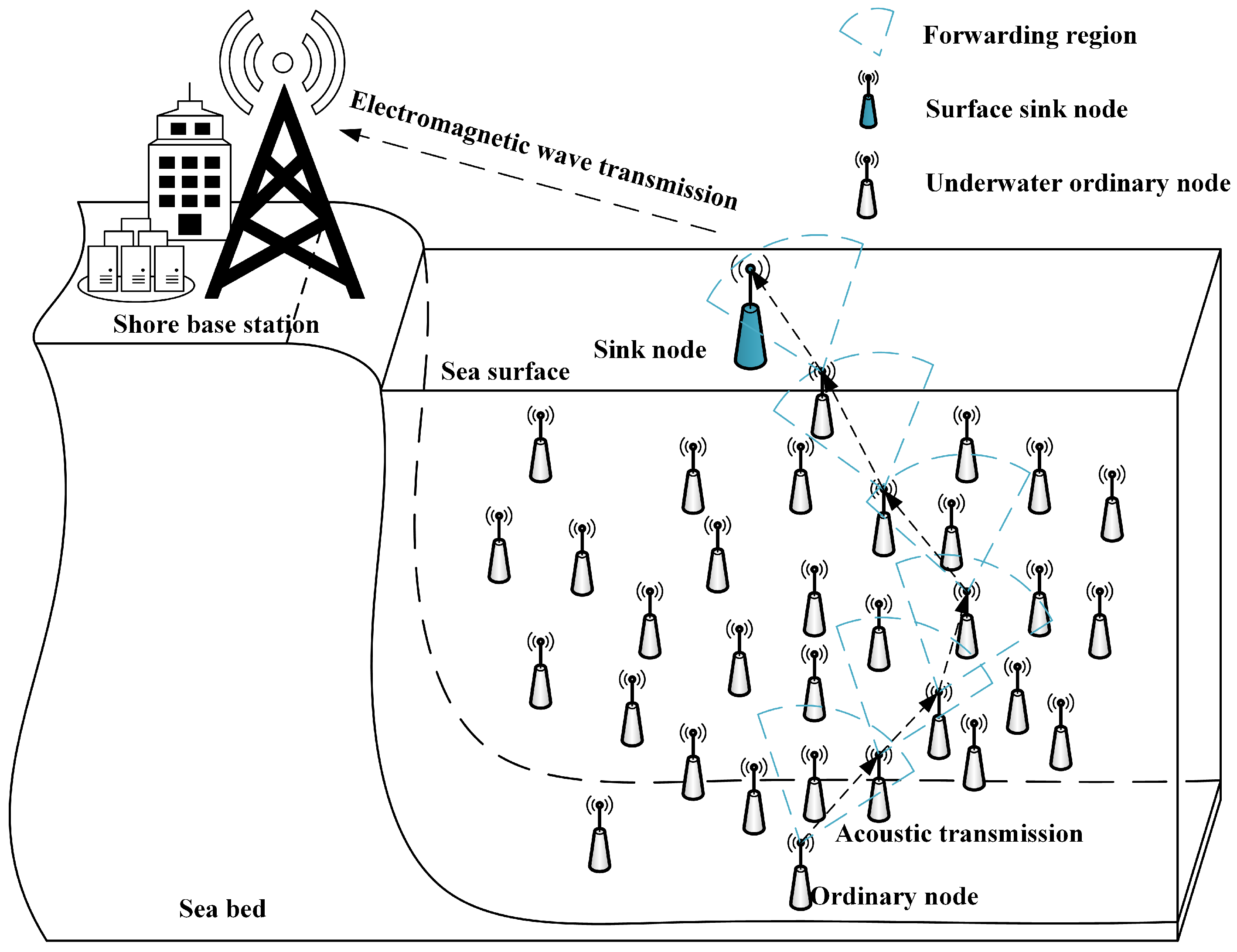
The FLRAF routing protocol utilizes the network architecture depicted in Figure 1, which comprises ordinary sensor nodes, sink nodes, and a shore-based station. The ordinary sensor nodes, which are responsible for data collection, are dispersed randomly within a 3D space. The sink nodes, fixed on the ocean surface, gather the data collected by the ordinary sensor nodes. Consequently, after receiving the acoustic data transmitted from ordinary sensor nodes in a hop-by-hop manner, the sink nodes aggregate the information and relay it via electromagnetic waves to the shore station for subsequent processing and analysis.

2.2. Network Model of the FLRAF

The transmission attenuation of the underwater acoustic signal depends on center frequency and transmission distance. In this paper, we use the Urick model to characterize the underwater acoustic signal’s propagation loss [36], which can be expressed as

$$A(d,f)=d^k\alpha {\left(f\right)}^{{\displaystyle \frac{d}{1000}}}$$

(1)

where d represents the Euclidean distance between nodes (in m), k is the spreading factor describing the propagation geometry with a value ranging from 1 to 2, typically set to 1.5, f denotes the acoustic carrier frequency (in kHz), and $\alpha \left(f\right)$ represents the absorption coefficient.

For the Euclidean distance d between nodes, $N_i(x_i,y_i,z_i)$ is used to represent the 3D coordinates of any node and $d_{i,j}$ can be used to represent the Euclidean distance between any two nodes. The calculation formula is as follows:

$$d_{i,j}=\sqrt{{(x_i-x_j)}^2+{(y_i-y_j)}^2+{(z_i-z_j)}^2}.$$

(2)

We note that a variety of underwater localization technologies have been extensively studied and applied, which can effectively mitigate the impact of signal distortion on localization accuracy. These technologies provide a solid foundation to ensure the feasibility of position-based forwarding strategies in practical scenarios [37,38].

The absorption coefficient $\alpha \left(f\right)$ can be determined according to Thorp’s empirical formula [36], which is calculated as

$$10{log}_{10}\alpha \left(f\right)=0.003+{\displaystyle \frac{0.11f^2}{1+f^2}}+{\displaystyle \frac{44f^2}{4100+f^2}}+{\displaystyle \frac{2.75f^2}{{10}^4}}.$$

(3)

Besides path loss, underwater acoustic signals face interference from ocean noise during transmission. Ocean noise $N\left(f\right)$ comprises various components, which can be broadly categorized into the following environmental noise sources: shipping noise $N_s\left(f\right)$, turbulence noise $N_t\left(f\right)$, thermal noise $N_{th}\left(f\right)$, and wave noise $N_w\left(f\right)$. The calculation can be determined using

$$\begin{array}{cc}\hfill N\left(f\right)& =N_t\left(f\right)+N_s\left(f\right)+N_w\left(f\right)+N_{th}\left(f\right)\hfill \end{array}$$

(4)

$$\begin{array}{cc}\hfill 10{log}_{10}{N}_t\left(f\right)& =17-30{log}_{10}f\hfill \end{array}$$

(5)

$$\begin{array}{cc}\hfill 10{log}_{10}{N}_s\left(f\right)& =40+20(s-0.5)+26{log}_{10}f\hfill \\ \hfill & -60{log}_{10}(f+0.03)\hfill \end{array}$$

(6)

$$\begin{array}{cc}\hfill 10{log}_{10}{N}_w\left(f\right)& =50+7.52\sqrt{w}+20{log}_{10}f\hfill \\ \hfill & -40{log}_{10}(f+0.4)\hfill \end{array}$$

(7)

$$\begin{array}{cc}\hfill 10{log}_{10}{N}_{th}\left(f\right)& =-15+20{log}_{10}f\hfill \end{array}$$

(8)

where s represents the shipping activity factor, which is a constant ranging from 0 to 1, typically set to s = 0.8, and w is the speed of wind (in m/s) set according to specific conditions.

After obtaining the transmission loss of the underwater acoustic signal, if only path transmission loss and noise interference are considered, the $SNR$ between nodes can be estimated using

$$SNR(d,f)={\displaystyle \frac{P}{A(d,f)N\left(f\right)}}$$

(9)

where P represents the transmitted acoustic source power (in $\mathrm{dB}/\mu \mathrm{Pa}$) and $N\left(f\right)$ denotes the noise power spectral density. It is important to note that nodes convert electrical signals into acoustic signals to transmit data via underwater acoustic transducers. The conversion between the transmitted acoustic source power and the electrical transmission power is determined by

$$10{log}_{10}P=10{log}_{10}\tilde{P}+170.8+10{log}_{10}\eta$$

(10)

where $\eta$ is the efficiency of the underwater acoustic transducer, represented as a constant between 0 and 1, typically set to $\eta$ = 0.8, $\tilde{P}$ is the electrical transmitting power (in W).

In this study, the acoustic characteristics of the transmission channel are primarily considered through the conversion between electrical power and acoustic source power, along with modeling the attenuation properties of sound propagation in underwater environments. Detailed structural-acoustic properties of the transducers and propagation interfaces are not explicitly modeled. In contrast, recent studies such as [39] have provided a more comprehensive analysis of vibroacoustic behavior by considering the sound transmission loss (STL) characteristics in lattice sandwich structures. Such detailed modeling offers valuable insights that can serve as a useful reference for our future research directions involving physical-layer acoustic modeling.

2.3. Forwarding Area of FLRAF

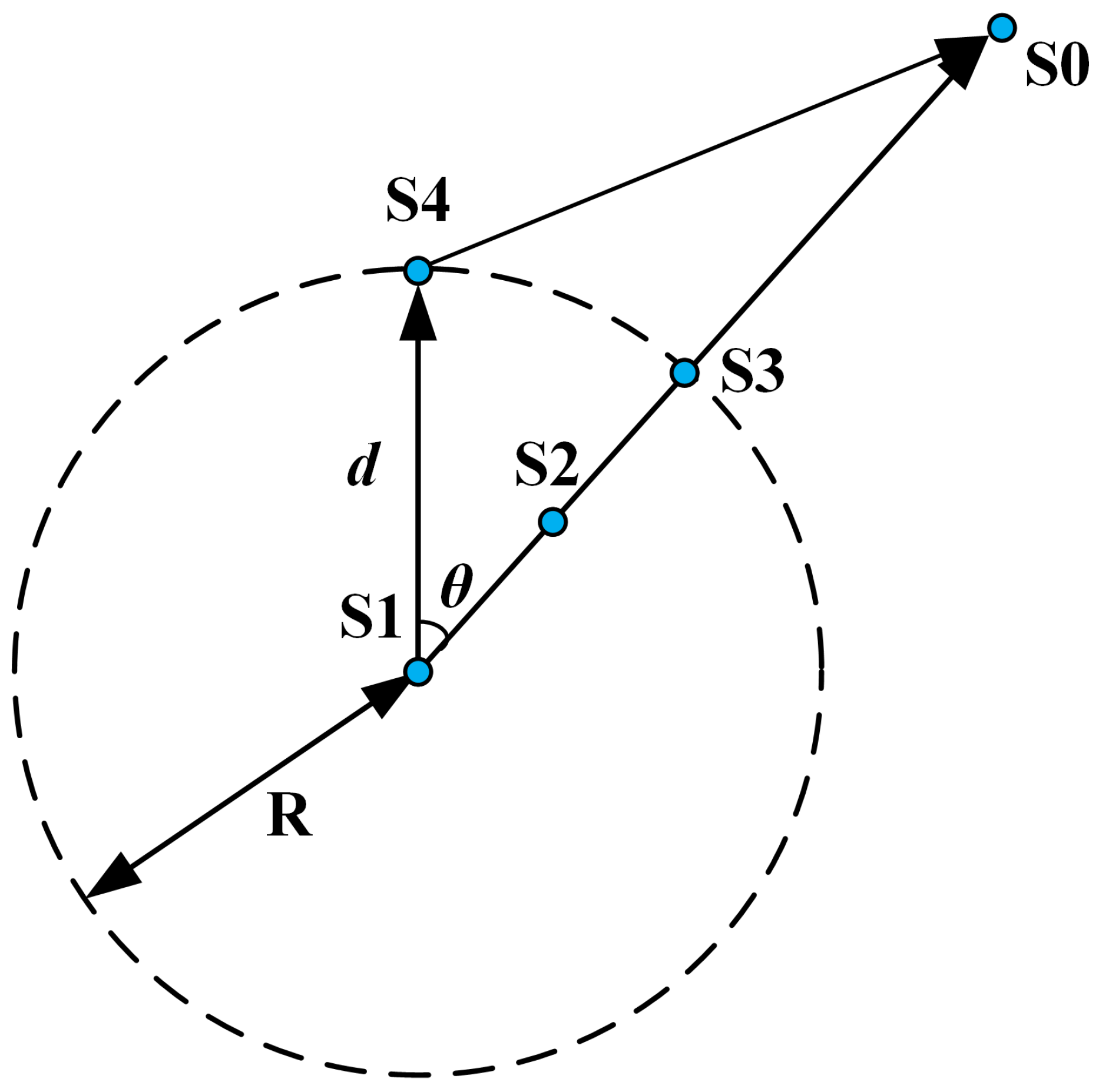
Figure 2 shows the one-hop transmission range scenario of UASN data transmission, where node S0 is the sink node and node S1 is the current forwarding node. If S4 is selected as the next hop forwarding node, the effective advance distance $AD$ is defined as

$$AD=d\times cos\theta .$$

(11)

From the perspective of the Thorp propagation model, when data are transmitted via multiple hops to the final sink node, maximizing $AD$ for each hop will minimize the end-to-end delay and the number of hops from the data transmission standpoint. Consequently, this approach provides benefits in both energy efficiency and transmission latency.

Specifically, as shown in Figure 2, when node S2 is located on the line connecting nodes S1 and S3, within the one-hop transmission range of S1 with a radius of R, S1 can directly send data to S3. It can also relay data through forwarding node S2. These two forwarding schemes have different energy consumption levels. Assuming the received signal power is $P_0$, according to Equation (9), the node transmission power is $A(d,f)N\left(f\right)P_0$. For the two mentioned data transmission schemes, we can use

$$\begin{array}{cc}\hfill E_{\mathrm{single}}& =A(d_{1,3},f)N\left(f\right)P_0{T}_{tx}+E_{elec}\hfill \\ \hfill & =N\left(f\right)P_0{T}_{tx}{d_{1,3}}^k{10}^{{\displaystyle \frac{a\left(f\right)d_{1,3}}{10}}}+E_{elec}\hfill \end{array}$$

(12)

$$\begin{array}{cc}\hfill E_{\mathrm{multiple}}& =A(d_{1,2},f)N\left(f\right)P_0{T}_{tx}+A(d_{2,3},f)N\left(f\right)P_0{T}_{tx}\hfill \\ & +2E_{elec}\hfill \\ \hfill & =N\left(f\right)P_0{T}_{tx}{d_{1,2}}^k{10}^{{\displaystyle \frac{a\left(f\right)d_{1,2}}{10}}}\hfill \\ & +N\left(f\right)P_0{T}_{tx}{d_{2,3}}^k{10}^{{\displaystyle \frac{a\left(f\right)d_{2,3}}{10}}}+2E_{elec}\hfill \end{array}$$

(13)

to represent the energy consumed by single-hop transmission and multihop transmission within the one-hop transmission range, where $E_{elec}$ denotes the energy required for the electronic equipment of the transmitter and receiver and $T_{tx}$ represents the transmission time of a data packet. Assuming that multihop transmission is more energy-efficient, then

$$d_{1,3}{10}^{{\displaystyle \frac{a\left(f\right)d_{1,3}}{10}}}-d_{1,2}{10}^{{\displaystyle \frac{a\left(f\right)d_{1,2}}{10}}}-d_{2,3}{10}^{{\displaystyle \frac{a\left(f\right)d_{2,3}}{10}}}>{\displaystyle \frac{E_{elec}}{N\left(f\right)P_0{T}_{tx}}}.$$

(14)

When node S2 lies on the line connecting nodes S1 and S3, there is $d_{1,3}=d_{1,2}+d_{2,3}$; otherwise, there is $d_{1,3}<d_{1,2}+d_{2,3}$. In terms of communication hardware, we choose the commonly used underwater acoustic modem model UWM1000 (LinkQuest Inc., San Diego, CA, USA) [40]. After our verification, obviously, Equation (14) is not valid, that is to say, within the one-hop transmission range, $E_{\sin \mathrm{gle}}<E_{\mathrm{multiple}}$, extended to the whole network range, in order to maintain the optimal energy consumption, it is necessary to ensure as few multihop transmission hops as possible. When the current forwarding node is S1, nodes S3 and S4 are within the one-hop transmission range, but $A{D}_{\mathrm{S}3}>A{D}_{\mathrm{S}4}$; therefore, to ensure as few multihop transmission hops as possible, nodes with larger $AD$ within the forwarding node should be selected. To further constrain the forwarding node and make the forwarding area contain as many nodes with larger $AD$ as possible, we redefine the geometric boundary and selection criteria of the forwarding area, as shown in the blue area in Figure 3.

The forwarding area of node A can be represented as

$$\left\{\begin{array}{l}{(x-x_0)}^2+{(y-y_0)}^2+{(z-z_0)}^2\le R^2\hfill \\ cos\left(\gamma \right)\le {\displaystyle \frac{\overrightarrow{\mathrm{AB}}·\overrightarrow{\mathrm{AD}}}{\left|\overrightarrow{\mathrm{AB}}\right|\times \left|\overrightarrow{\mathrm{AD}}\right|}}\hfill \end{array}\right.$$

(15)

where the coordinates $(x_0,y_0,z_0)$, $(x_1,y_1,z_1)$, $(x_2,y_2,z_2)$, and $(x,y,z)$ denote the positional information for forwarding node A, sink node B, node C in the previous hop’s forwarding region, and location D shown in Figure 3. $\gamma$ is the semi-vertex angle of the “cone” forwarding area. When the node position $(x,y,z)$ satisfies Equation (15), it can be determined that the node is in the forwarding area of the previous forwarding node. Since the vertex of the “cone” forwarding area is at $\mathrm{A}(x_0,y_0,z_0)$, the axis is along $\overrightarrow{\upsilon }=\overrightarrow{\mathrm{AB}}=(x_1-x_0,y_1-y_0,z_1-z_0)$, and the semi vertex angle is $\gamma$, we only need to ensure that the angle $\beta$ between the vector $\overrightarrow{\omega }$ from the center of the sphere $\mathrm{A}(x_0,y_0,z_0)$ to the point $\mathrm{C}(x,y,z)$ and the “cone” axis vector $\overrightarrow{\upsilon }$ is less than or equal to $\gamma$. We have

$$cos\left(\beta \right)={\displaystyle \frac{\overrightarrow{\omega }·\overrightarrow{\upsilon }}{\left|\overrightarrow{\omega }\right|\times \left|\overrightarrow{\upsilon }\right|}}$$

(16)

and let $cos\left(\gamma \right)\le cos\left(\beta \right)$, finally let

$${(x-x_0)}^2+{(y-y_0)}^2+{(z-z_0)}^2\le R^2.$$

(17)

That is to say, A needs to be confined within the sphere. In addition, to determine the scope of the optimal forwarding area in the future, it is agreed here that $\alpha ={\displaystyle \frac{\gamma }{{90}^{\circ }}}$.

2.4. Evaluation of Link Quality Between Nodes

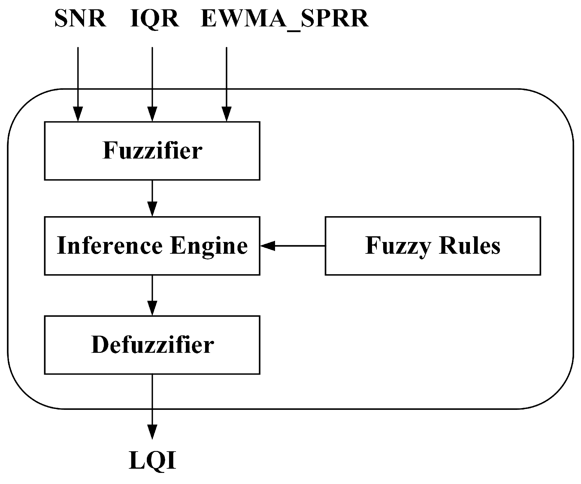
A fuzzy logic reasoning system is an intelligent system that uses fuzzy logic for reasoning and decision making. Its functions include processing uncertainty, fuzzy information, and complex multidimensional data. The implementation process of fuzzy reasoning usually includes fuzzification, rule-based reasoning, and defuzzification steps. This system is commonly applied in fields such as automatic control, pattern recognition, intelligent transportation systems, and wireless sensor networks. Through precise evaluation and decision making, the efficiency and reliability of the system are improved. In this section, we constructed an inner layer fuzzy logic reasoning system to complete the evaluation task of inter-node link quality, as shown in Figure 4.

In addition to the $SNR$ mentioned in Equation (9), the input to the fuzzy inference system also includes two other parameters: the interquartile range ($IQR$) of the cumulative $PRR$ at different time points and the smoothed $PRR$ obtained through exponentially weighted moving average processing ($EWMA\_SPRR$). The rationale behind selecting these two parameters is as follows. First, we do not use the coefficient of variation ($CV$) of $PRR$ because it is highly sensitive to fluctuations in link quality at a single time instant, which may lead to misleading results. For instance, a momentary degradation in link quality can cause a significant drop in $PRR$, thereby introducing substantial variations in the computed $CV$. In contrast, the $IQR$ is more robust to transient fluctuations, as it primarily reflects the dispersion of the middle 50% of the data points. This makes $IQR$ a more stable metric for assessing long-term link quality while filtering out short-term variations. Additionally, we calculate the $EWMA\_SPRR$ because it provides a predictive capability. By assigning exponentially decreasing weights to past observations, the $EWMA\_SPRR$ value enables a smoother estimation of $PRR$ trends, allowing for a more reliable prediction of future link quality based on historical data. This predictive aspect is particularly beneficial in dynamic underwater acoustic environments, where link quality can fluctuate due to various factors, such as mobility, multipath effects, and environmental disturbances.

$SNR$ reflects the real-time physical channel quality and serves as a primary indicator of potential signal distortion due to environmental noise. Higher $SNR$ values generally imply more favorable transmission conditions. However, due to the inherent volatility of underwater channels, relying solely on instantaneous $SNR$ may lead to unstable decision making. $IQR$ of $PRR$ captures the dispersion of $PRR$ values over a predefined observation window, quantifying the consistency and stability of the link performance. A smaller $IQR$ implies a more stable link, while a larger $IQR$ indicates fluctuating reception quality and potential unreliability due to transient disturbances such as mobility or interference. $EWMA\_SPRR$ introduces a smoothing mechanism that emphasizes recent $PRR$ trends while still considering historical observations. This exponentially weighted average enhances temporal robustness, mitigating the effects of outliers or sudden dips caused by momentary channel degradation.

The fuzzy inference mechanism leverages the degree of membership of these parameters to predefined fuzzy sets (e.g., High $SNR$, Low $IQR$, Good $EWMA\_SPRR$) and integrates them through fuzzy rules to output an aggregated $LQI$ value, which reflects both instantaneous and long-term link quality trends. This design aims to reduce susceptibility to short-term fluctuations and provide a more resilient and adaptive link assessment model for routing decisions. That is to say, by integrating $IQR$ and $EWMA\_SPRR$, our approach effectively balances robustness against transient fluctuations and adaptability to long-term link quality trends, enhancing the reliability of our routing decisions. Assuming we have obtained the $PRR$ values at the current time point t and n previous time points, we will take the obtained 10 $PRR$ values (assuming they are already arranged from small to large) as an example to introduce the calculation process of the $IQR$. First, arrange the data from small to large, and then find the positions of the 25th and 75th percentiles of the data, namely the lower quartile $Q1$ and upper quartile $Q3$:

$$\begin{array}{cc}\hfill & Q_1=PR{R}_2+0.5\times (PR{R}_3-PR{R}_2)\hfill \end{array}$$

(18)

$$\begin{array}{cc}\hfill & Q_3=PR{R}_7+0.5\times (PR{R}_8-PR{R}_7).\hfill \end{array}$$

(19)

The final $IQR$ is:

$$IQR=Q_3-Q_1.$$

(20)

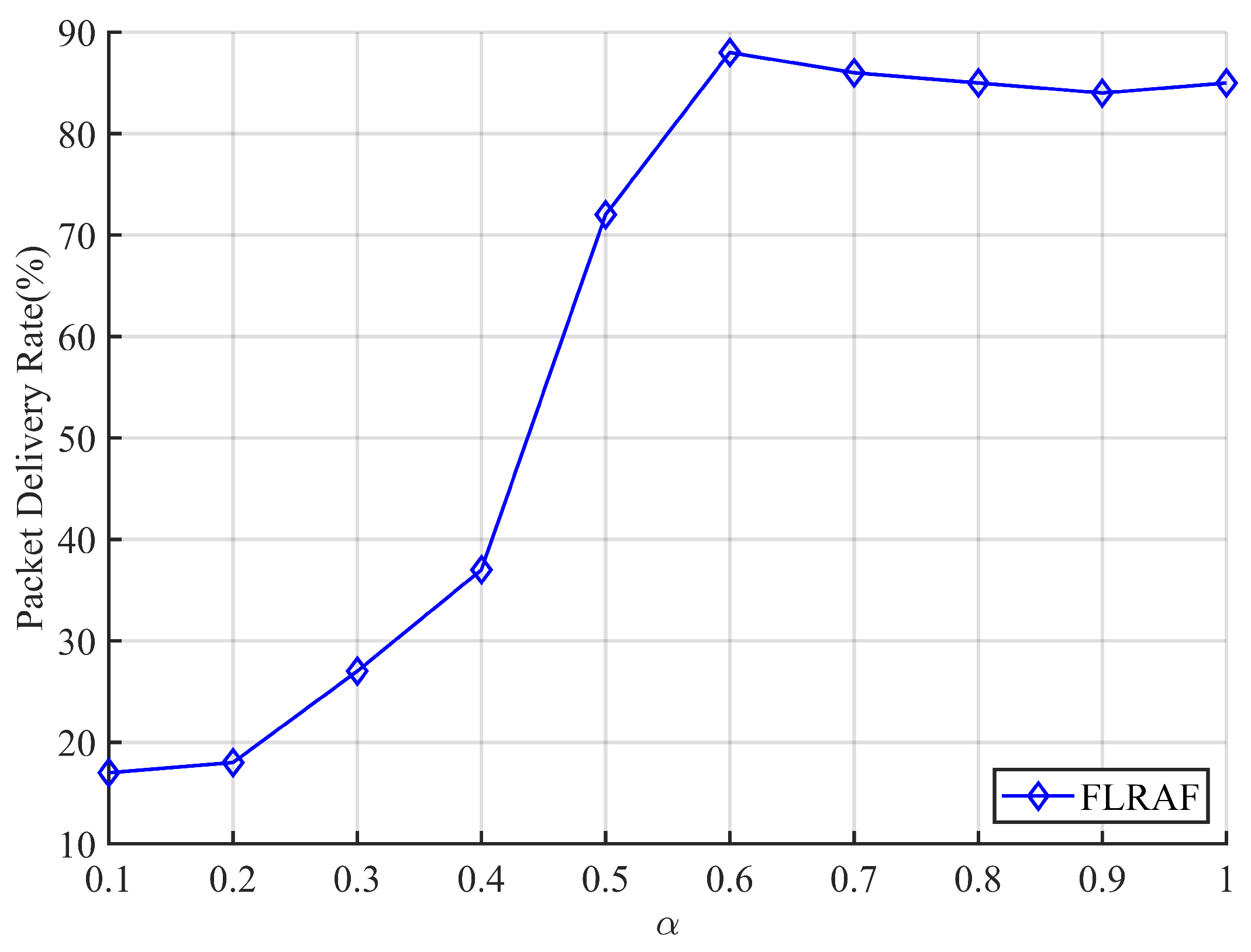
Additionally, calculate $EWMA\_SPRR$ using the following recursive formula:

$$EWMA\_SPR{R}_t=\lambda \times EWMA\_SPR{R}_{t-1}+(1-\lambda )PR{R}_t$$

(21)

where $\lambda$ controls the smoothness of the weighted moving average.

Furthermore, although the current evaluation environment assumes relatively stable underwater acoustic conditions, the proposed fuzzy-logic-based routing protocol exhibits strong adaptability to dynamic environmental factors such as temperature gradients, water currents, and multipath propagation effects. The modular structure of the fuzzy inference system allows for seamless integration of additional environment-aware parameters, such as signal delay spread or Doppler shift estimates, which can further enhance link quality assessment accuracy. This design flexibility ensures that the protocol remains robust and scalable even in complex and time-varying underwater acoustic environments, laying a solid foundation for future improvements in highly dynamic application scenarios.

Figure 5 illustrates the process of obtaining the $LQI$. The detailed application of the fuzzy logic reasoning system is further addressed in the subsequent design of the outer-layer fuzzy reasoning system, which is used to prioritize candidate sets in the opportunistic routing and forwarding area.

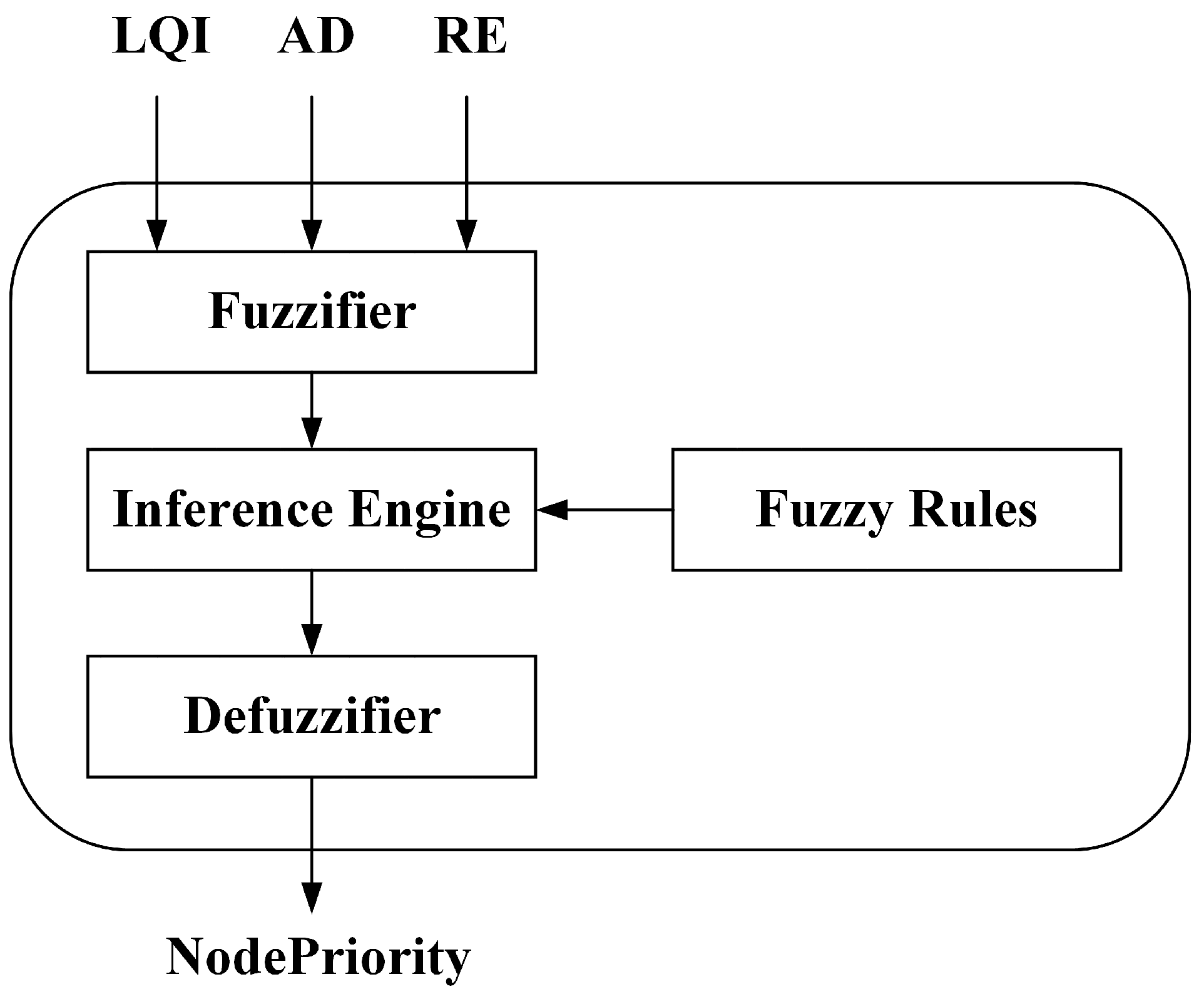
2.5. Fuzzy Logic Reasoning Selection of Candidate Set

The outer layer fuzzy reasoning system comprehensively considers three parameters: node residual energy $RE$, which affects the final network lifetime; link quality index $LQI$, which affects the final packet delivery rate; and effective advance distance $AD$ of nodes, which affects the multihop forwarding efficiency, to participate in the outer layer fuzzy reasoning. That is to say, the $LQI$ represents the communication reliability of the node’s link to the next hop and directly impacts the packet delivery ratio. Prioritizing nodes with higher $LQI$ ensures stable and successful data transmission. The $RE$ level reflects the remaining battery capacity of the node. Giving higher forwarding priority to nodes with greater energy reserves contributes to balanced energy consumption across the network and helps extend the overall network lifetime. The $AD$ level is a spatial metric that promotes efficient data propagation. Nodes with larger forward progress are generally closer to the destination, reducing the number of required hops and potentially minimizing end-to-end transmission delay. This metric implicitly promotes low-latency routing, which is especially critical in delay-sensitive underwater applications. The schematic diagram of the outer layer fuzzy reasoning is shown in Figure 6.

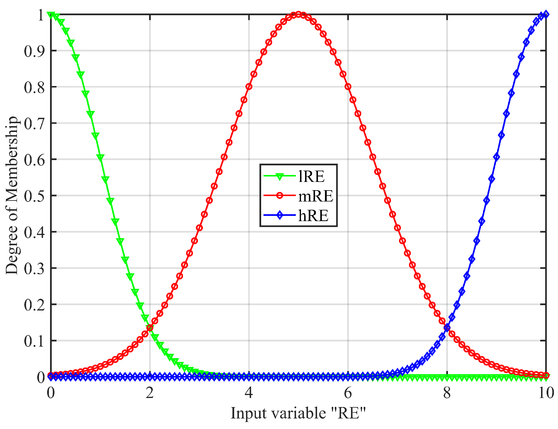
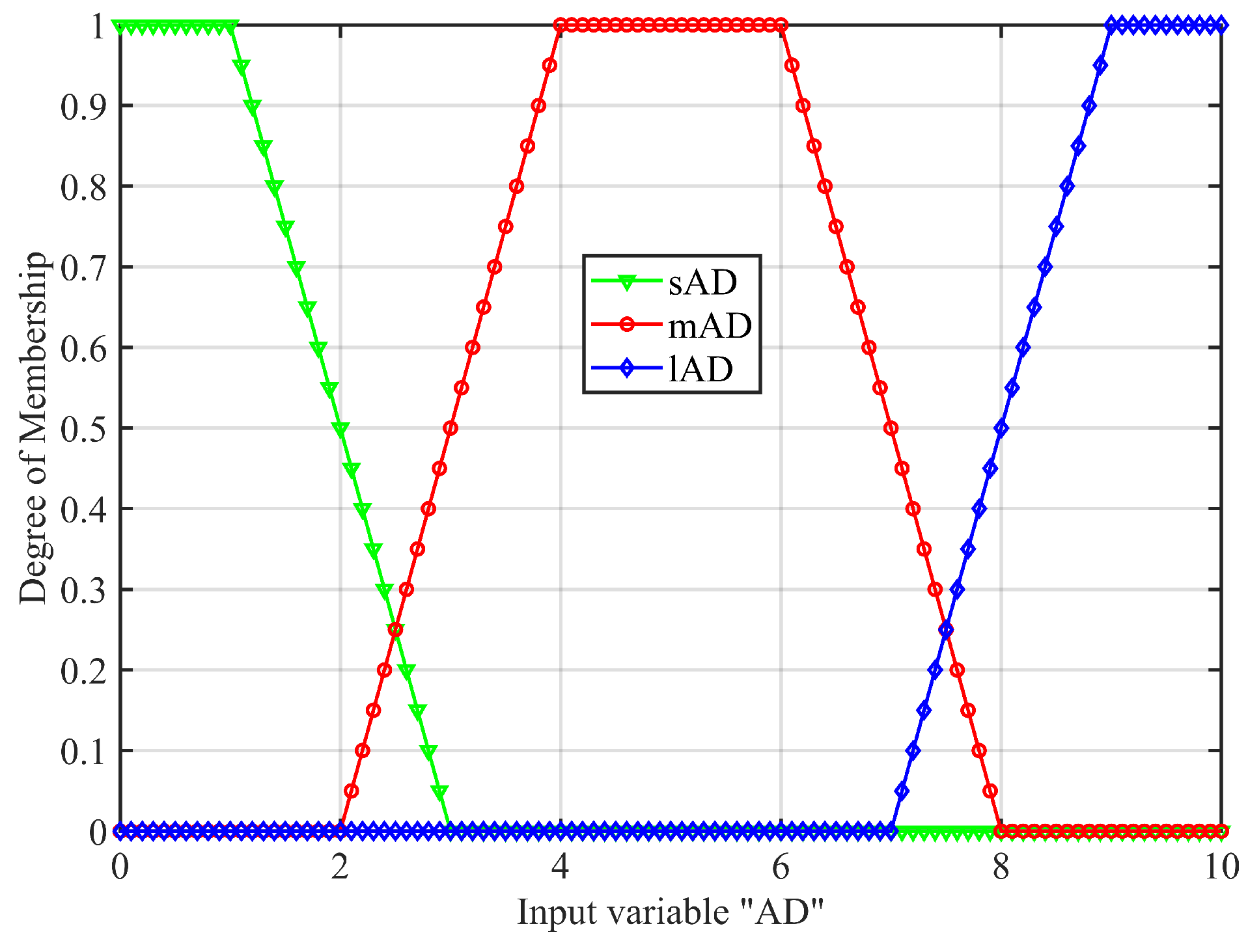
The specific process of building a fuzzy logic reasoning system to complete specific design tasks can be roughly summarized into four steps. First, clarify the design problem, the input and output of the system, and their possible range of variation. The outer fuzzy inference system takes into account three parameters: the link quality index $LQI$ that affects the final data packet delivery rate; the nodes’ remaining energy $RE$ that affects the final network lifetime; and the effective advance distance $AD$ of the nodes that affect the multihop forwarding efficiency to participate in the outer layer fuzzy inference. To make the weights of multiple fuzzy inputs more balanced and improve the performance of the model, the original fuzzy input data are first linearly mapped to a specified range. Given an original data point x, we aim to map it to a new range $\left[a,b\right]$, which can be linearly mapped according to the following formula:

$$x_{normalize}=a+{\displaystyle \frac{(x-x_{min})\times (b-a)}{x_{max}-x_{min}}}.$$

(22)

We plan to map the original fuzzy input to a new range $\left[0,10\right]$, so we take $a=0,b=10$.

Next, we determine the number of fuzzy subsets for the input and output variables. The number of fuzzy subsets is related to the granularity of the fuzzy inference. Based on the types of fuzzy subsets, the corresponding membership functions are established. In this case, each of the three fuzzy input variables is assigned three fuzzy subsets. The respective membership functions are then configured accordingly. The detailed configuration is presented in

Table 1. Fuzzy subsets and membership function types corresponding to fuzzy inputs and output.

Fuzzy Variables	Variables Name	Fuzzy Subsets Classification	Types of Membership Function
Fuzzy inputs	RE	lRE (low RE)	Gaussian
		mRE (medium RE)	Gaussian
		hRE (high RE)	Gaussian
	LQI	bLQI (bad LQI)	Triangular
		mLQI (medium LQI)	Triangular
		gLQI (good LQI)	Triangular
	AD	sAD (short AD)	Trapezoidal
		mAD (medium AD)	Trapezoidal
		lAD (long AD)	Trapezoidal
Fuzzy output	NodePriority	vlPriority (very low Priority)	Triangular
		lPriority (low Priority)	Triangular
		mPriority (medium Priority)	Triangular
		hPriority (high Priority)	Triangular
		vhPriority (very high Priority)	Triangular

.

Table 1 shows the membership functions for the fuzzy subset of the four variables. It is worth mentioning that the determination of the membership function for fuzzy variables corresponding to fuzzy subsets requires comprehensive consideration. Generally, fuzzy sets can be classified into three types: small-type, medium-type, and large-type. For example, “low node energy” represents a small-type fuzzy set, where the membership degree increases as the energy value decreases, indicating a worse node energy state. Conversely, “high node energy” represents a large-type fuzzy set, where the membership degree increases with higher energy values, indicating a better node energy state. “Moderate node energy” represents a medium-type fuzzy set, where the membership degree is highest when the energy value falls within a certain intermediate range. In summary, it is important to consider the relationship between “elements” and “membership degree”, which implies the monotonicity of the membership function. This is essential to ensure that the fuzzy inference process produces logically consistent and semantically accurate outputs. If this relationship is not properly considered, the system may yield misleading evaluations. For instance, if a “low node energy” fuzzy set were mistakenly designed with a membership degree that increases with increasing energy, then a node with extremely low energy might be falsely assigned a low membership degree, misleading the system to treat it as a high-energy node and prioritize it for data forwarding—thereby accelerating energy depletion and reducing network lifetime. Therefore, appropriate membership function design is crucial for ensuring the correctness and robustness of the fuzzy inference system. Additionally, the use of different membership functions for the three other fuzzy input variables effectively avoids the feature representation blind spots that may arise from using a single function type. The resulting membership function graphs are shown in Figure 7, Figure 8, Figure 9, and Figure 10, respectively.

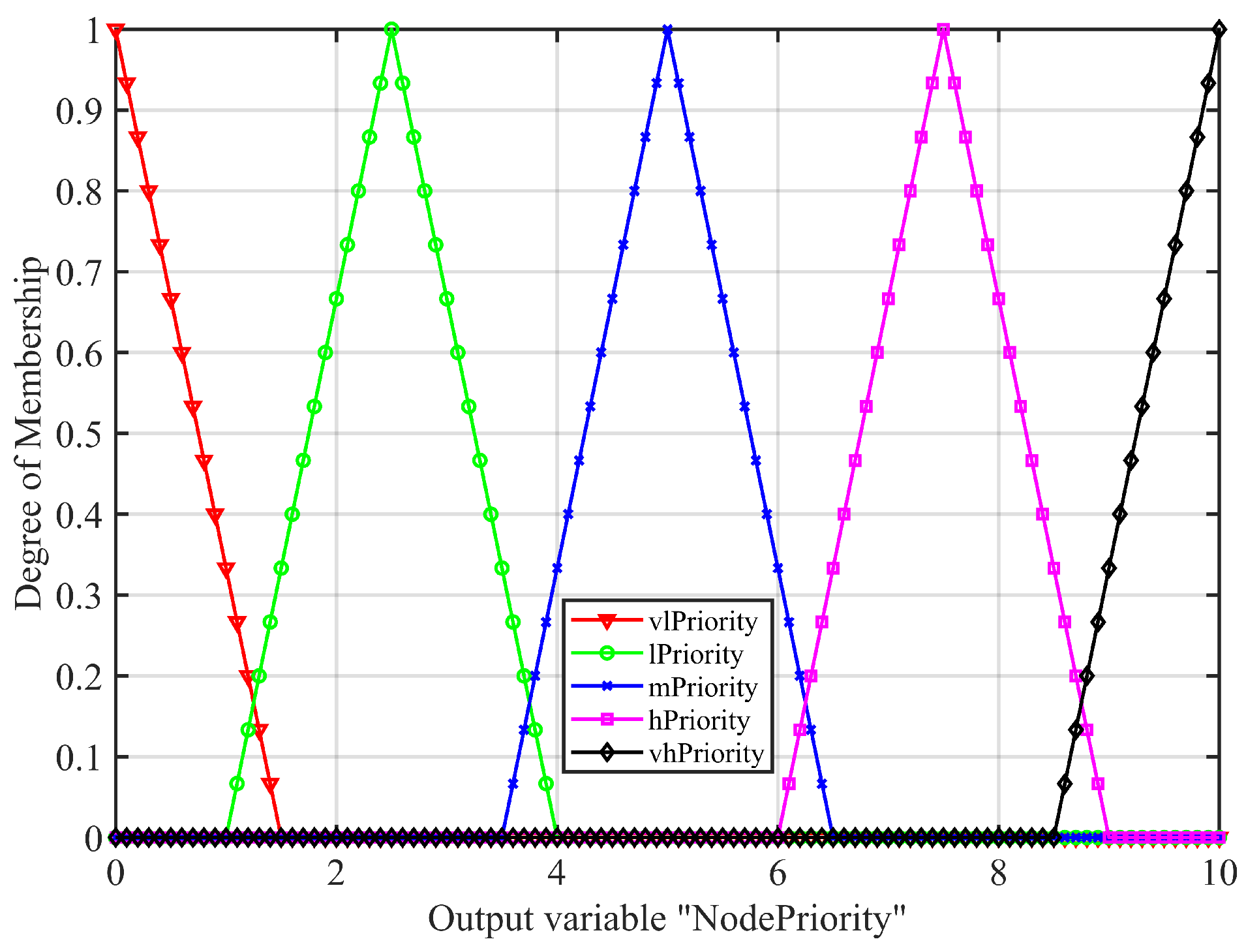
Second, according to the system design requirements, we set inference rules. Since we have set fuzzy logic inputs for three variables and each fuzzy input has three fuzzy subsets, we can exhaustively list all possible inference rules; however, due to space limitations, only a subset of the fuzzy reasoning rules is shown in

Table 2. Partial fuzzy reasoning rules.

Rule Number	Rule
rule 1	If RE is lRE and AD is sAD and LQI is gLQI then NodePriority is bPriority
rule 2	If RE is mRE and AD is sAD and LQI is gLQI then NodePriority is mPriority
rule 3	If RE is hRE and AD is sAD and LQI is gLQI then NodePriority is gPriority
rule 4	If RE is lRE and AD is mAD and LQI is gLQI then NodePriority is mPriority
rule 5	If RE is mRE and AD is mAD and LQI is gLQI then NodePriority is mPriority
rule 6	If RE is hRE and AD is mAD and LQI is gLQI then NodePriority is gPriority
rule 7	If RE is lRE and AD is lAD and LQI is gLQI then NodePriority is gPriority
…	…

.

In fact, if we broadly define the three fuzzy subsets of fuzzy input as “good”, “medium”, and “poor”, then the fuzzy inference rules can be broadly categorized as follows:

(1)

If all three fuzzy inputs are “good”, then the fuzzy output is “vhPriority”;

(2)

If all three fuzzy inputs are “poor”, then the fuzzy output is “vlPriority”;

(3)

If any two fuzzy inputs are “good”, the fuzzy output is “hPriority”;

(4)

If any two fuzzy inputs are “medium”, the fuzzy output is “mPriority”;

(5)

If any two fuzzy inputs are “poor”, the fuzzy output is “lPriority”;

(6)

If the three fuzzy inputs are, respectively, “good”, “medium”, and “poor”, the fuzzy output is “mPriority”.

Finally, the fuzzy reasoning system progresses to the defuzzification process, where the Centroid defuzzification method is used to obtain the final fuzzy output. Assuming two candidate nodes exist within the forwarding area at the same time, their node state information is [8 8 2] and [8 8 9], respectively, (i.e., using [$REi$ $ADi$ $LQIi$] to represent the state information of node i). After processing by our nested fuzzy inference system, the priorities of the two nodes are 6.82 and 8.59, respectively. Therefore, the FLRAF routing protocol tends to choose the latter as the forwarding node, because the former indicates that the node has good remaining energy and a long effective advance distance, but poor link quality, while the latter indicates that the node has excellent link quality, sufficient remaining energy, and long effective advance distance. On the other hand, when conducting fuzzy logic reasoning, different reasoning rules can also be assigned different weights to maximize their compatibility with the designer’s specific needs.

2.6. Forwarding Process of the FLRAF

The specific forwarding process of the FLRAF routing protocol is described as follows. First, during network initialization, the sink node broadcasts a data collection query, which is divided into location-based queries and queries that define event-triggering conditions. The former broadcasts data packets carrying the geographic location of interest to all nodes in the network, while the latter broadcasts data packets carrying events of interest to the sink node (such as whether the temperature in the area exceeds the threshold) to all nodes in the network. Through this step of processing, nodes know whether they need to start the data collection task. This preliminary step significantly reduces unnecessary energy consumption by allowing only relevant nodes to participate in data forwarding.

Second, each node that receives the query will determine its one-hop forwarding area based on the predefined geometric constraints and establish a candidate set of neighboring nodes. Using a fuzzy logic reasoning mechanism that comprehensively evaluates factors such as residual energy, link quality, and distance to the sink, the optimal forwarding node is identified. The selected node is responsible for transmitting the data, while other nodes in the candidate set discard the received data to avoid redundant transmissions and conserve energy. This decision-making process ensures both energy efficiency and robustness in dynamic underwater environments.

The forwarding node then transmits the data in a hop-by-hop manner, repeating the candidate selection and fuzzy inference at each step, until the data eventually reach the sink node. Finally, the sink node gathers the desired information and forwards it to the shore-based control station via its equipped radio modems for further analysis and processing. The complete forwarding process of the FLRAF routing protocol and the information that needs to be exchanged in each part to complete the forwarding task are shown in Figure 11 and

Table 3. Packet format in the FLRAF routing protocol forwarding process.

Packet Format Serial Number	Task Type/Information Carried by the Packet
Format 0	Initiate LQI acquisition task/Current forwarder’s location
Format 1	Initiate data collection task/Sink’s location, query type
Format 2	Initiate data collection task/Node i’s forwarding area
Format 3	Initiate fuzzy logic reasoning task/Receiver’s ID
Format 4	Report reasoning result/Receiver’s ID, node priority
Format 5	Report node selection result/Forwarder’s ID, data collected
Format 6	Terminate redundant transmissions and initiate data collection of a new round/node i’s forwarding area, node j’s forwarding area

.

3. Performance Evaluation Results and Discussion

3.1. Simulation Environment

We carried out our simulation work in the underwater acoustic simulator Aqua-sim-NG, aiming to compare and analyze the FLRAF routing protocol we proposed with existing traditional protocols, including VBF, HH-VBF, ALRP, and GTRP. We conduct a thorough assessment to determine whether the proposed protocol offers advantages by analyzing the effects of two scenario parameters—specifically, the number of nodes and their maximum movement speed—on four common network performance metrics. To ensure a fair comparison and consistency with previous studies, the simulation parameters are set based on [25,26], where similar settings have been validated. The main network simulation scenario parameters are set as shown in

Table 4. Major parameters used in the simulation.

Parameters	Value
Routing protocol	VBF, HH-VBF, ALRP, GTRP, FLRAF
MAC layer protocol	Broadcast MAC
Propagation model	Underwater Propagation
Channel	Underwater Channel
Number of nodes	100–600
Node transmission range	100 m
Simulation time	500 s
Size of simulation scene	800 m × 800 m × 800 m
Moving model	RandomWalkMobilityModel
Maximum moving speed of node	2–7 m/s
Application layer data rate	3 kbps
VBF, HH-VBF radius of pipe	70 m
Node transmit, receive and idle power	2.0 W, 0.75 W, 0.008 W
k, $T_{delay}$ in ALRP	7, 1 s
$\beta$ in GTRP	${10}^6$
$\alpha$ in FLRAF	0.6

.

Additionally, all protocols are tested under identical network configurations and simulation durations to eliminate bias in performance evaluation. The selected performance metrics include average end-to-end delay, packet delivery ratio, average energy consumption, and lifetime, which comprehensively reflect the protocol’s adaptability, reliability, and efficiency in dynamic underwater environments. Through this simulation setup, we aim to rigorously verify the practical effectiveness and robustness of the FLRAF protocol under varying network conditions.

3.2. Performance Metrics

This study assesses the effectiveness of routing protocols by analyzing their performance across four common network parameters, namely network average energy consumption $E_{average}$, network average end-to-end delay $Avdelay$, packet delivery rate $PDR$, and network lifetime. $E_{average}$ can be calculated as

$$E_{average}={\displaystyle \frac{{\displaystyle \sum _{j=1}^{N_{pit}}}{E}_j}{P_r}}$$

(23)

where $E_j$ is the energy consumption of each participating node and $N_{pit}$ is the number of nodes involved in the network transmission process.

$Avdelay$ can be calculated as

$$Avdelay={\displaystyle \frac{{\displaystyle \sum _{i=1}^{P_r}}(r_{time}\left(i\right)-s_{time}\left(i\right))}{P_r}}$$

(24)

where $s_{time}\left(i\right)$ and $r_{time}\left(i\right)$ are the times when the i-th data packet is sent from the source node and arrives at the sink node, respectively.

$PDR$ is calculated as

$$PDR={\displaystyle \frac{P_r}{P_s}}$$

(25)

where $P_r$ represents the number of successfully received data packets at the sink node and $P_s$ denotes the number of packets transmitted by the source node.

Finally, network lifetime is defined as the duration from the start of the simulation until the first node depletes its energy.

3.3. Effects of $\alpha$ on the FLRAF

An excessively large or overly small forwarding area can lead to corresponding problems. For example, when the forwarding area is too small, it may be difficult to locate a suitable next-hop node, potentially resulting in routing voids and data transmission interruptions. Conversely, when the forwarding area is too large, the overall energy consumption of the network tends to increase. Therefore, simulation experiments were conducted to determine the optimal forwarding area. As shown in Figure 3, we agreed that the angle $\gamma$ is the half vertex angle of the “cone” forwarding area, and $\alpha ={\displaystyle \frac{\gamma }{{90}^{\circ }}}$, that is, $\alpha =0$ corresponds to $\gamma =0^{\circ }$ and $\alpha =1$ corresponds to $\gamma ={90}^{\circ }$. The subsequent simulation phase focuses on examining how variations in $\alpha$ affect the performance of the FLRAF protocol. We varied $\alpha$ from 0.1 to 1 in order to identify the optimal value and to compare the performance of the FLRAF protocol with other existing protocols under these conditions. To complete this simulation work, we will set the simulation parameters as shown in

Table 5. Simulation parameters for optimal forwarding area verification.

Parameters	Value
Routing protocol	FLRAF
MAC layer protocol	Broadcast MAC
Propagation model	Underwater Propagation
Channel	Underwater Channel
Number of nodes	400
Node transmission range	100 m
Simulation time	500 s
Size of simulation scene	800 m × 800 m × 800 m
Moving model	RandomWalkMobilityModel
Maximum moving speed of node	4 m/s
Application layer data rate	3 kbps
Node transmit, receive and idle power	2.0 W, 0.75 W, 0.008 W
$\alpha$ in FLRAF	0.1–1

.

Figure 12 shows the impact of $\alpha$ on the delivery rate of data packets. First, the figure shows that as $\alpha$ increases, the forwarding area expands, leading to a rise in the number of nodes within this area. Consequently, the probability of routing voids or transmission interruptions decreases accordingly. As a result, the number of received data packets will increase. After $\alpha >0.7$, the delivery rate begins to stabilize and slightly decline. This is because the forwarding area becomes sufficiently large, and there are already enough nodes available to participate in the forwarding process. Thanks to the fuzzy reasoning process, we choose nodes with better states to act as forwarding nodes. However, even if we further increase the forwarding area and add more nodes, the members located near the forwarding node of the previous hop are not suitable to form a candidate set. Therefore, they have a minimal positive impact on the final packet delivery rate. On the contrary, the increased node density may lead to more data collisions, which can negatively affect the packet delivery rate.

Figure 13 illustrates the impact of $\alpha$ on the average end-to-end delay. When $\alpha <0.3$, the forwarding area is still at a relatively small level, and the number of candidate nodes contained in the forwarding area is also limited. At this time, the routing path may be longer, or the next-hop candidate node may not be found, resulting in increased delay caused by transmission interruptions. As $\alpha$ increases, on the one hand, the number of candidate nodes available for the previous-hop node increases; on the other hand, more nodes with longer $AD$ appear in the candidate area. Therefore, the delay will be significantly reduced. Finally, due to the mobility of the nodes, there is a slight change in their relative position, and similar to the reason resulting in the trend of $PDR$ in Figure 12, there is a slight increase in latency caused by data collisions.

Figure 14 shows the impact of $\alpha$ on the average energy consumption of the network. When the delivery rate is at a lower level, the network does not reduce energy consumption, but a small number of received data packets will inevitably result in a higher average energy consumption. Therefore, when $\alpha <0.3$, due to the limited number of received data packets, the average energy consumption is at a relatively high level, but as the forwarding area increases, the success rate of data transmission gradually increases, while the average energy consumption decreases as it is gradually averaged. On the other hand, after $\alpha >0.6$, the forwarding area gradually expands, involving a greater number of nodes in the forwarding process, thus increasing the overall energy consumption. The slight decrease in the number of received data packets further contributes to a slight increase in average energy consumption.

Figure 15 shows the effect of $\alpha$ on the network lifetime. Thanks to the fuzzy reasoning system we introduced, we effectively avoided the possibility of selecting low-energy nodes as forwarding nodes in the early stage. As $\alpha$ increases, the range of the forwarding area also increases, and more nodes will be included. The more nodes there are, the longer the time interval for a single node to serve as a forwarding node, and with a fixed initial energy of the node, the number of network simulation rounds it participates in will increase, thereby extending the network lifetime. The network lifetime will theoretically continue to extend as the number of nodes grows.

Therefore, after comprehensively analyzing the impact of changes in forwarding regions on the performance of various network parameters, we found that when $\alpha =0.6$, the data delivery rate remains high, while both average energy consumption and end-to-end delay perform well. Therefore, we ultimately determined $\alpha =0.6$ as the optimal forwarding area configuration, and conducted performance parameter simulations comparing our proposed FLRAF protocol with other existing protocols in the following sections.

3.4. Effects of the Node Density

The simulation work here aims to explore the impact of changes in the number of nodes on protocol performance. The variation range of the number of nodes in this simulation is 100–600, and Table 4 shows other necessary simulation parameters.

Figure 16 shows the trend of packet delivery rate of different protocols with varying numbers of nodes. The packet delivery rate of the five protocols gradually increases with the increase in the number of nodes. The reason is that the node number significantly affects network density. When the node density is low, the number of nodes contained in the forwarding area of each forwarding node is also quite small, which may cause a routing void and interrupt data transmission. Traditional protocols have not taken specific measures to address the routing void, resulting in a lower packet reception success rate. This is a common problem that may be encountered when the network density is low. The FLRAF protocol can evaluate the link quality between nodes to select nodes with good transmission conditions, but it cannot effectively address the issue of routing void. Therefore, when the number of nodes is small, a high data packet delivery rate cannot be guaranteed either. As node density rises, more nodes are available in each forwarding area, which boosts the chances of the routing protocol successfully finding the next hop node. Therefore, the problem of data transmission interruption will be greatly improved, and the packet delivery rate will gradually increase.

Figure 17 shows the trend of the network average end-to-end delay of different protocols as the number of nodes changes. Thanks to the fuzzy reasoning system added to the FLRAF protocol, the effective advance distance is taken into account when selecting nodes. Therefore, in the process of selecting nodes, nodes at the edge of the transmission range are given more priority while maximizing compliance with the SNR requirement. This may maximize the efficiency of multihop transmission by reducing the number of hops that data packets pass through from source to sink. Thus, the FLRAF method reduces the average end-to-end delay compared to most traditional protocols. However, its delay performance is inferior to the GTRP method due to the use of fuzzy reasoning in evaluating link quality. It is necessary to transmit probe packets to complete the task of evaluating link quality. This process introduces additional processing delay, partially offsetting FLRAF’s advantage in reducing transmission latency. This is a problem that needs to be considered in the later stage.

Figure 18 shows the trend of network average energy consumption of different protocols with varying numbers of nodes. In terms of energy consumption, as the number of nodes increases, the total energy consumption of the network will inevitably increase gradually. This is because, in the process of one-hop transmission, the higher the network density, the greater the number of nodes involved in receiving the data packets sent by the forwarding nodes of the previous hop, which will inevitably result in higher energy consumption. On the other hand, because the average energy consumption of the network is determined by dividing the total energy consumption of the network by the number of data packets successfully received by the receiving node, and due to the difference in the speed of increase between the total energy consumption of the network and the number of successfully received data packets, the average energy consumption shows a gradual upward trend.

Figure 19 shows the trend of the network lifetime of different protocols with varying numbers of nodes. The network lifetime extends with the increase of the number of nodes. Traditional protocols do not have a node selection process for energy management, and the network lifetime will not change significantly. This is due to the protocol relying solely on node location information during selection. Therefore, as the network continues to operate without other intervention, there may be one or several nodes frequently serving as forwarding nodes, which will accelerate node depletion. When selecting nodes in the FLRAF protocol, the output layer fuzzy reasoning system is considered to evaluate the priority of candidate nodes. When the node energy is low, the fuzzy logic output value is small, indicating that the node is no longer suitable for serving as a forwarding node. Therefore, this method indirectly achieves the function of nodes taking turns to serve as forwarding nodes, which significantly helps to prolong the network lifetime.

3.5. Impacts of Maximum Speed of Nodes

Figure 20 shows the trend of the packet delivery rate of different protocols when the maximum movement speed of a node changes. During the simulation process, the most fundamental problem introduced by node movement is the fluctuation in the number of candidate nodes within the forwarding area. Because the forwarding area is relatively fixed, some nodes may move out of the original area due to the randomly assigned positions. However, because of the variability in movement speed, the number of nodes in the forwarding area remains relatively stable in actual simulations. For example, when the number of nodes in the entire network is set to 400, the number of nodes in a single-hop forwarding area is about 10. Therefore, due to the introduction of the mobility model, there may be an increase or decrease in the number of nodes in the actual forwarding area. The impact of node mobility on network performance is equivalent to the variation in network parameters when the number of nodes ranges from 200 to 500. Thus, node movement has a minimal effect on the packet reception success rate, showing only minor fluctuations.

Figure 21 shows the trend of network average end-to-end delay of different protocols as the maximum movement speed of nodes changes. Except for the VBF protocol, which is sensitive to node movement due to the use of a single pipeline forwarding area, the other four protocols show a slightly increasing trend. The reason is also that the two-dimensional movement model of random walks superimposes movement speed and direction, which causes fluctuations in the number of nodes within the forwarding region. Therefore, the number of nodes at the optimal forwarding position or the edge of the transmission range will decrease, thus reducing the effective advance distance of one-hop transmission and increasing the number of end-to-end transmission hops, thereby increasing the overall end-to-end delay.

Figure 22 shows the trend of network average energy consumption across different protocols as the maximum node movement speed varies. When a node joins or escapes from the original forwarding area due to mobility, node density within the forwarding region changes, which in turn affects the number of nodes involved in receiving the data packets from the previous forwarding node, which will impact the overall energy consumption performance of the network. As shown in Figure 20, the number of successfully received data packets is also fluctuating, so the average energy consumption of the network will also show slight fluctuations. This is jointly determined by the trend of total energy consumption and the number of successfully received data packets in the network.

Figure 23 shows the trend of the network lifetime across different protocols as the maximum node movement speed varies. Similarly, when node density within the forwarding area changes due to node movement, for example, if a new node joins the forwarding area, the time interval for the node to take turns serving as a forwarding node in one-hop transmission will increase. When the node’s initial energy is constant, the time interval for the node to act twice as a forwarding node will increase. This is because there are more nodes participating in the “rotation” process. Therefore, for a single node, its survival time will be extended. Conversely, when a node escapes from the original forwarding area, the network survival time will correspondingly decrease. Due to the random superposition of node movement speed, the overall trend of network survival time also fluctuates.

4. Conclusions

This study introduces a novel routing protocol designed for 3D UASNs, utilizing fuzzy logic reasoning to enhance performance, as it is well suited to handling fuzzy input variables related to node state information, such as “high residual energy”, “high advance distance”, etc. We first conducted a theoretical analysis and found that the fewer hops packets experienced, the better the energy efficiency of the network. Therefore, we establish a new forwarding area to maximize multihop forwarding efficiency and reduce redundant transmission. Equally important is how to adaptively select suitable forwarding nodes based on node spatial distribution and state information, which will directly affect the transmission delay and parameters related to the energy consumption of the network.

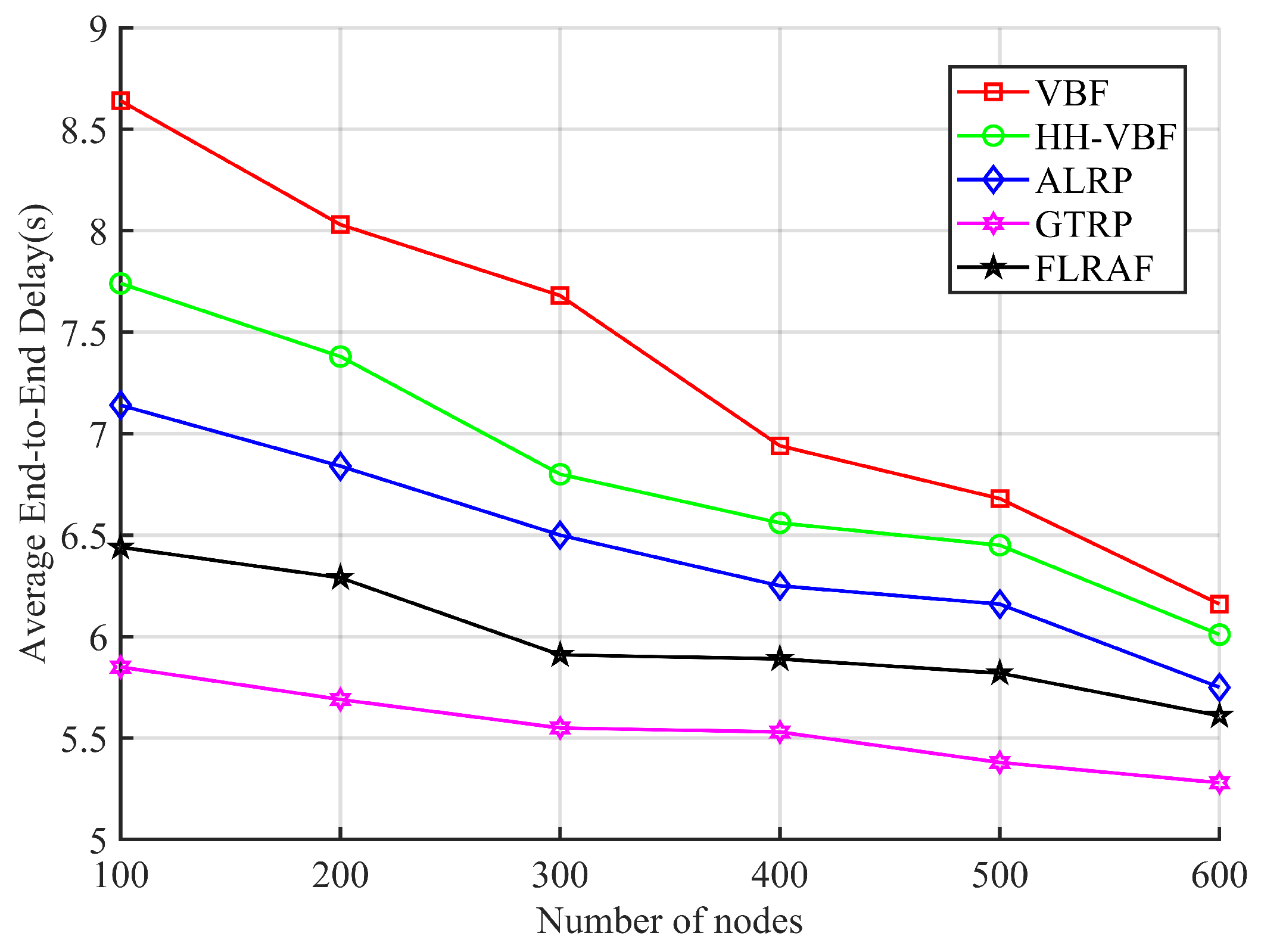
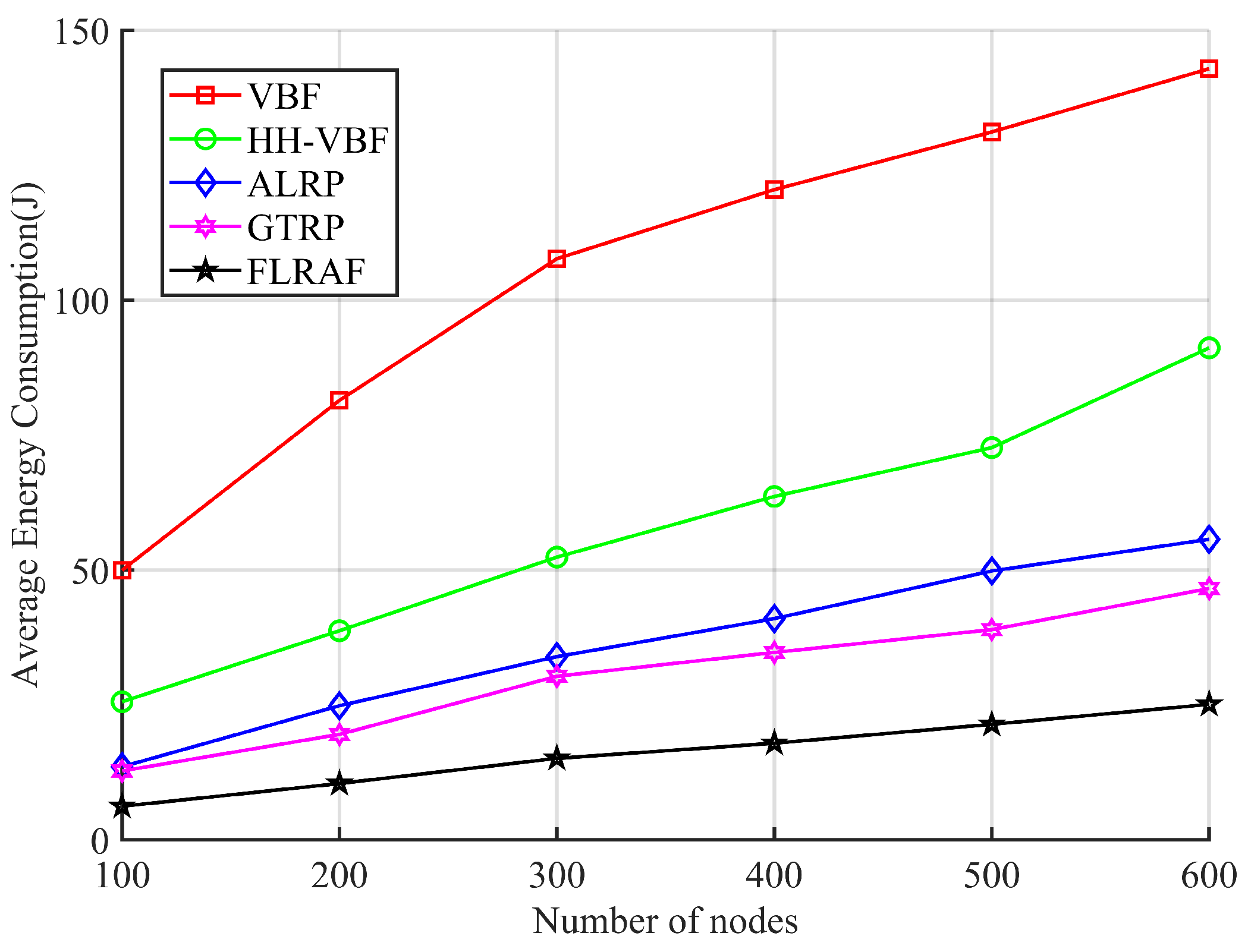
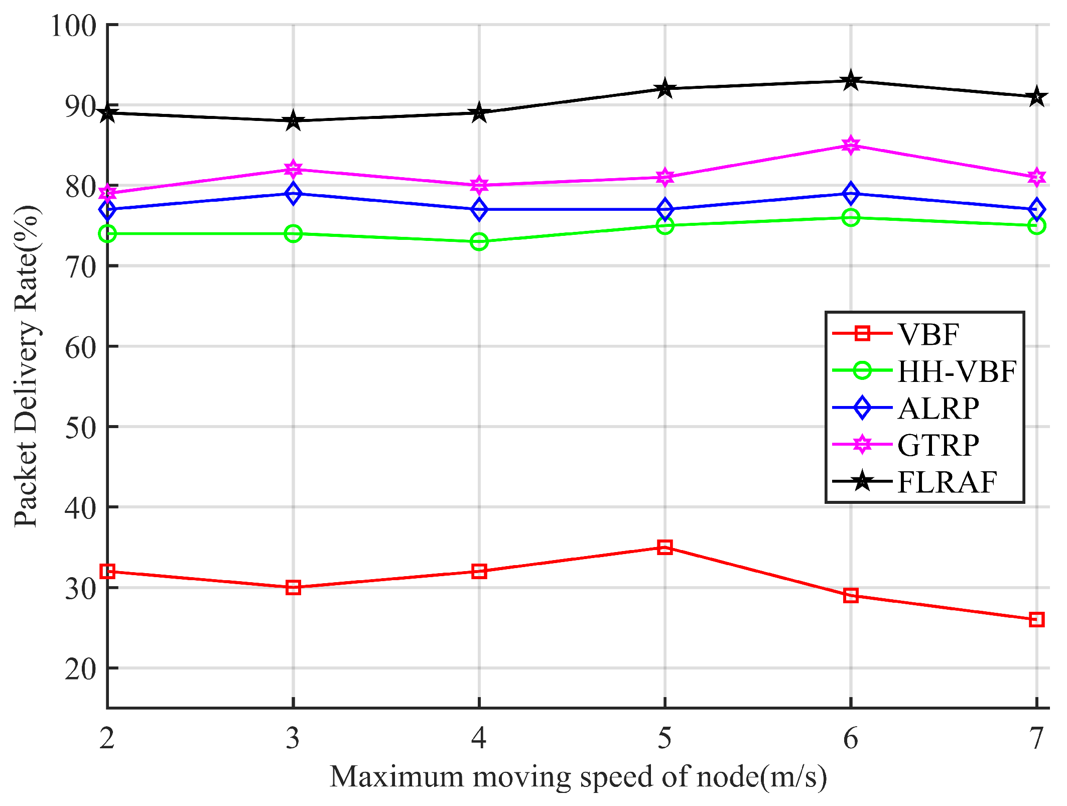
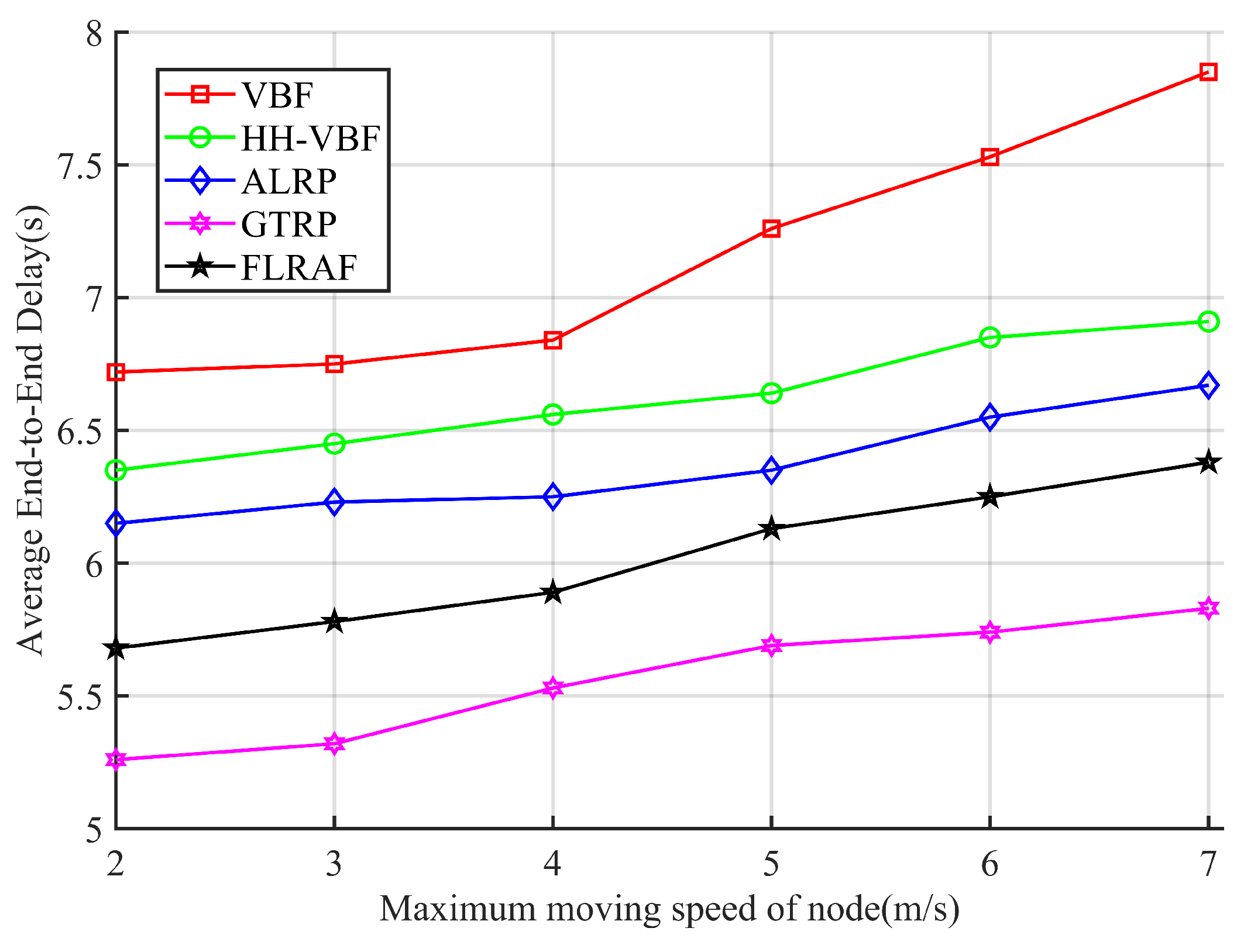
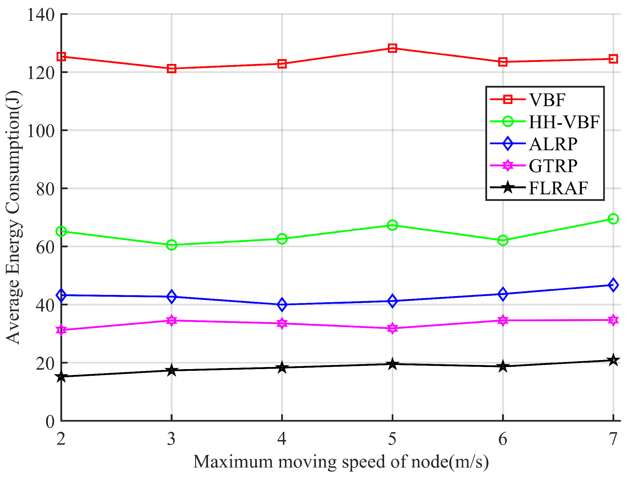
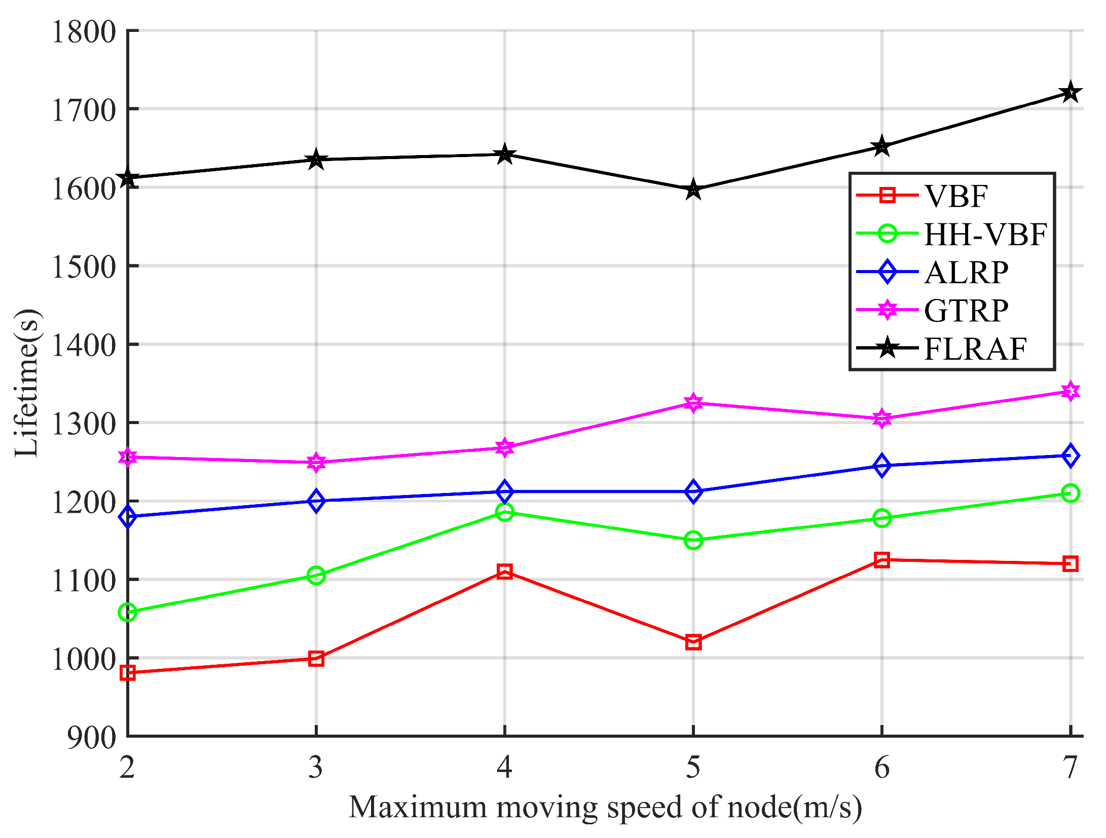
Through numerous simulations and validations, our proposed protocol demonstrates clear advantages over existing protocols in terms of average energy consumption, packet delivery rate, and network lifespan. On the one hand, it is due to the forwarding area we have established, which fundamentally reduces the possibility of inappropriate nodes acting as forwarding nodes. On the other hand, it is due to the outer fuzzy inference system we have designed, which reduces the possibility of a single node frequently acting as a forwarding node. This is very effective for extending the network lifetime. However, the performance of the FLRAF routing protocol in average end-to-end delay is not yet outstanding because it is necessary to transmit probe packets to complete the task. This process introduces unnecessary processing delay, which offsets the advantage of the FLRAF protocol in reducing transmission delay. Another important source of propagation delay is the priority evaluation task within the candidate set. After a node completes the final fuzzy reasoning, it reports the priority evaluation result to the next-hop forwarding node. This forms a many-to-one data transmission scenario. The original Broadcast MAC protocol is unable to effectively coordinate data transmission conflicts, leading to data collisions and the accumulation of propagation delay. The next step is to design a MAC protocol that can coordinate data transmission. For instance, an RTS frame containing queue length and data transmission time information is sent to the central node. The central node calculates the waiting time for node data transmission and encapsulates the coordination scheme into a CTS frame. Nodes then follow the coordination scheme to perform data transmission, thereby minimizing data collisions as much as possible. This is a problem that needs to be addressed in our subsequent research.

References

1. Chettri, L.; Bera, R. A comprehensive survey on Internet of Things (IoT) toward 5G wireless systems. IEEE Internet Things J. 2019, 7, 16–32. [Google Scholar] [CrossRef]
2. Islam, M.M.; Nooruddin, S.; Karray, F.; Muhammad, G. Internet of things: Device capabilities, architectures, protocols, and smart applications in healthcare domain. IEEE Internet Things J. 2022, 10, 3611–3641. [Google Scholar]
3. Prajapat, R.; Yadav, R.N.; Misra, R. Energy-efficient k-hop clustering in cognitive radio sensor network for internet of things. IEEE Internet Things J. 2021, 8, 13593–13607. [Google Scholar]
4. Su, Y.; Liwang, M.; Gao, Z.; Huang, L.; Du, X.; Guizani, M. Optimal cooperative relaying and power control for IoUT networks with reinforcement learning. IEEE Internet Things J. 2020, 8, 791–801. [Google Scholar]
5. Bello, O.; Zeadally, S. Internet of underwater things communication: Architecture, technologies, research challenges and future opportunities. Ad Hoc Netw. 2022, 135, 102933. [Google Scholar] [CrossRef]
6. Jahanbakht, M.; Xiang, W.; Hanzo, L.; Azghadi, M.R. Internet of underwater things and big marine data analytics—A comprehensive survey. IEEE Commun. Surv. Tutor. 2021, 23, 904–956. [Google Scholar]
7. Zhou, G.; Wang, Z.; Li, Q. Spatial Negative Co-Location Pattern Directional Mining Algorithm with Join-Based Prevalence. Remote Sens. 2022, 14, 2103. [Google Scholar] [CrossRef]
8. Zhao, D.; Mao, W.; Chen, P.; Hu, Y.; Liang, H.; Dang, Y.; Liang, R.; Guo, X. A distributed and parallel accelerator design for 3-D acoustic imaging on FPGA-based systems. IEEE Trans. Comput.-Aided Des. Integr. Circuits Syst. 2023, 43, 1401–1414. [Google Scholar]
9. Han, G.; Huang, Y.; He, Y.; Li, F.; Li, A.; Peng, J. A Data Transmission Scheme Based on Reinforcement Learning-Aided Two-Stage Trust Evaluation for UASNs. IEEE Internet Things J. 2024, 11, 35155–35166. [Google Scholar]
10. Al Guqhaiman, A.; Akanbi, O.; Aljaedi, A.; Chow, C.E. A survey on MAC protocol approaches for underwater wireless sensor networks. IEEE Sens. J. 2020, 21, 3916–3932. [Google Scholar]
11. Zhang, H.; Shen, H. Balancing energy consumption to maximize network lifetime in data-gathering sensor networks. IEEE Trans. Parallel Distrib. Syst. 2008, 20, 1526–1539. [Google Scholar]
12. Javaid, N.; Karim, O.A.; Sher, A.; Imran, M.; Yasar, A.U.H.; Guizani, M. Q-Learning for energy balancing and avoiding the void hole routing protocol in underwater sensor networks. In Proceedings of the 2018 14th International Wireless Communications & Mobile Computing Conference (IWCMC), Limassol, Cyprus, 25–29 June 2018; pp. 702–706. [Google Scholar]
13. Coutinho, R.W.; Boukerche, A.; Vieira, L.F.; Loureiro, A.A. EnOR: Energy balancing routing protocol for underwater sensor networks. In Proceedings of the 2017 IEEE International Conference on Communications (ICC), Paris, France, 21–25 May 2017; pp. 1–6. [Google Scholar]
14. Heinzelman, W.R.; Chandrakasan, A.; Balakrishnan, H. Energy-efficient communication protocol for wireless microsensor networks. In Proceedings of the 33rd Annual Hawaii International Conference on System Sciences, Maui, HI, USA, 4–7 January 2000. [Google Scholar]
15. Faheem, M.; Tuna, G.; Gungor, V.C. QERP: Quality-of-service (QoS) aware evolutionary routing protocol for underwater wireless sensor networks. IEEE Syst. J. 2017, 12, 2066–2073. [Google Scholar]
16. Zhang, J.; Cai, M.; Han, G.; Qian, Y.; Shu, L. Cellular clustering-based interference-aware data transmission protocol for underwater acoustic sensor networks. IEEE Trans. Veh. Technol. 2020, 69, 3217–3230. [Google Scholar]
17. Awais, M.; Javaid, N.; Naseer, N.; Imran, M. Exploiting energy efficient routing protocols for void hole alleviation in IoT enabled underwater WSN. In Proceedings of the 2019 15th International Wireless Communications & Mobile Computing Conference (IWCMC), Tangier, Morocco, 24–28 June 2019; pp. 1797–1802. [Google Scholar]
18. Hwang, D.; Kim, D. DFR: Directional flooding-based routing protocol for underwater sensor networks. In Proceedings of the OCEANS 2008, Quebec City, QC, Canada, 15–18 September 2008; pp. 1–7. [Google Scholar]
19. Ahmed, S.H.; Lee, S.; Park, J.; Kim, D.; Rawat, D.B. iDFR: Intelligent directional flooding-based routing protocols for underwater sensor networks. In Proceedings of the 2017 14th IEEE Annual Consumer Communications & Networking Conference (CCNC), Las Vegas, NV, USA, 8–11 January 2017; pp. 560–565. [Google Scholar]
20. Yan, H.; Shi, Z.J.; Cui, J.H. DBR: Depth-based routing for underwater sensor networks. In NETWORKING 2008. Proceedings of the Ad Hoc and Sensor Networks, Wireless Networks, Next Generation Internet: 7th International IFIP-TC6 Networking Conference, Singapore, 5–9 May 2008; Springer: Berlin/Heidelberg, Germany, 2008; pp. 72–86. [Google Scholar]
21. Gul, S.; Jokhio, S.H.; Jokhio, I.A. Light-weight depth-based routing for underwater wireless sensor network. In Proceedings of the 2018 International Conference on Advancements in Computational Sciences (ICACS), Lahore, Pakistan, 19–21 February 2018; pp. 1–7. [Google Scholar]
22. Ali, M.; Khan, A.; Mahmood, H.; Bhatti, N. Cooperative, reliable, and stability-aware routing for underwater wireless sensor networks. Int. J. Distrib. Sens. Netw. 2019, 15, 1550147719854249. [Google Scholar]
23. Javaid, N.; Shakeel, U.; Ahmad, A.; Alrajeh, N.; Khan, Z.A.; Guizani, N. DRADS: Depth and reliability aware delay sensitive cooperative routing for underwater wireless sensor networks. Wirel. Netw. 2019, 25, 777–789. [Google Scholar]
24. Xie, P.; Cui, J.H.; Lao, L. VBF: Vector-based forwarding protocol for underwater sensor networks. In NETWORKING 2006. Proceedings of the Networking Technologies, Services, and Protocols; Performance of Computer and Communication Networks; Mobile and Wireless Communications Systems: 5th International IFIP-TC6 Networking Conference, Coimbra, Portugal, 15–19 May 2006; Springer: Berlin/Heidelberg, Germany, 2006; pp. 1216–1221. [Google Scholar]
25. Nicolaou, N.; See, A.; Xie, P.; Cui, J.H.; Maggiorini, D. Improving the robustness of location-based routing for underwater sensor networks. In Proceedings of the Oceans 2007-Europe, Aberdeen, UK, 18–21 June 2007; pp. 1–6. [Google Scholar]
26. Coutinho, R.W.; Boukerche, A.; Vieira, L.F.; Loureiro, A.A. Geographic and opportunistic routing for underwater sensor networks. IEEE Trans. Comput. 2015, 65, 548–561. [Google Scholar]
27. Wang, Q.; Li, J.; Qi, Q.; Zhou, P.; Wu, D.O. A game-theoretic routing protocol for 3-D underwater acoustic sensor networks. IEEE Internet Things J. 2020, 7, 9846–9857. [Google Scholar]
28. Wang, Q.; Li, J.; Qi, Q.; Zhou, P.; Wu, D.O. An Adaptive-Location-Based Routing Protocol for 3-D Underwater Acoustic Sensor Networks. IEEE Internet Things J. 2021, 8, 6853–6864. [Google Scholar]
29. Wang, L.; Fu, Q.; Zhu, R.; Liu, N.; Shi, H.; Liu, Z.; Li, Y.; Jiang, H. Research on high precision localization of space target with multi-sensor association. Optics Lasers Eng. 2025, 184, 108553. [Google Scholar]
30. Ding, F.; Wang, R.; Zhang, T.; Zheng, G.; Wu, Z.; Wang, S. Real-time trajectory planning and tracking control of bionic underwater robot in dynamic environment. Cyborg Bionic Syst. 2024, 5, 0112. [Google Scholar]
31. Zhao, D.; Zhou, H.; Chen, P.; Hu, Y.; Ge, W.; Dang, Y.; Liang, R. Design of forward-looking sonar system for real-time image segmentation with light multiscale attention net. IEEE Trans. Instrum. Meas. 2023, 73, 1–17. [Google Scholar]
32. Yang, L.; Lu, Y.; Yang, S.X.; Guo, T.; Liang, Z. A secure clustering protocol with fuzzy trust evaluation and outlier detection for industrial wireless sensor networks. IEEE Trans. Ind. Inform. 2020, 17, 4837–4847. [Google Scholar]
33. Kechiche, I.; Bousnina, I.; Samet, A. A novel opportunistic fuzzy logic based objective function for the routing protocol for low-power and lossy networks. In Proceedings of the 2019 15th International Wireless Communications & Mobile Computing Conference (IWCMC), Tangier, Morocco, 24–28 June 2019; pp. 698–703. [Google Scholar]
34. Baccour, N.; Koubâa, A.; Youssef, H.; Ben Jamâa, M.; Do Rosario, D.; Alves, M.; Becker, L.B. F-LQE: A fuzzy link quality estimator for wireless sensor networks. In Wireless Sensor Networks, Proceedings of the 7th European Conference, EWSN 2010, Coimbra, Portugal, 17–19 February 2010; Springer: Berlin/Heidelberg, Germany, 2010; pp. 240–255. [Google Scholar]
35. Li, G.; Zhang, Y.; Fan, S.; Yu, F.; Wang, Y. Dynamic-Wave Interference Suppression Based on Angular Increment Assistance for Underwater Imaging Polarization Sensor. IEEE Trans. Instrum. Meas. 2025, 74, 1–13. [Google Scholar]
36. Yu, H.; Yao, N.; Liu, J. An adaptive routing protocol in underwater sparse acoustic sensor networks. Ad Hoc Netw. 2015, 34, 121–143. [Google Scholar] [CrossRef]
37. Nain, M.; Goyal, N. Localization techniques in underwater wireless sensor network. In Proceedings of the 2021 International Conference on Advance Computing and Innovative Technologies in Engineering (ICACITE), Greater Noida, India, 4–5 March 2021; pp. 747–751. [Google Scholar]
38. Luo, J.; Yang, Y.; Wang, Z.; Chen, Y. Localization algorithm for underwater sensor network: A review. IEEE Internet Things J. 2021, 8, 13126–13144. [Google Scholar]
39. Jafari, M.H.A.; Zarastvand, M.; Zhou, J. Doubly curved truss core composite shell system for broadband diffuse acoustic insulation. J. Vib. Control 2024, 30, 4035–4051. [Google Scholar]
40. Bu, R.; Wang, S.; Wang, H. Fuzzy logic vector-based forwarding routing protocol for underwater acoustic sensor networks. Trans. Emerg. Telecommun. Technol. 2018, 29, e3252. [Google Scholar]
Figure 1. Network architecture for underwater acoustic sensor network (UASN) data collection.
Jmse 13 00692 g001
Figure 2. Node’s one-hop transmission range diagram.
Jmse 13 00692 g002
Figure 3. Schematic diagram of the forwarding area in the fuzzy logic reasoning adaptive forwarding (FLRAF) routing protocol.
Jmse 13 00692 g003
Figure 4. Schematic diagram of link quality index (LQI) acquisition process using inner layer fuzzy reasoning system.
Jmse 13 00692 g004
Figure 5. LQI acquisition process using inner layer fuzzy reasoning.
Jmse 13 00692 g005
Figure 6. Schematic diagram of node candidate priority acquisition process using outer layer fuzzy reasoning.
Jmse 13 00692 g006
Figure 7. The membership function of the fuzzy subset for the fuzzy input residual energy (RE).
Jmse 13 00692 g007
Figure 8. The membership function of the fuzzy subset for the fuzzy input LQI.
Jmse 13 00692 g008
Figure 9. The membership function of the fuzzy subset for the fuzzy input advance distance (AD).
Jmse 13 00692 g009
Figure 10. The membership function of the fuzzy subset for the fuzzy output NodePriority.
Jmse 13 00692 g010
Figure 11. FLRAF routing protocol forwarding process.
Jmse 13 00692 g011
Figure 12. Effects of α on packet delivery rate.
Jmse 13 00692 g012
Figure 13. Effects of α on average end-to-end delay.
Jmse 13 00692 g013
Figure 14. Effects of α on average energy consumption.
Jmse 13 00692 g014
Figure 15. Effects of α on network lifetime.
Jmse 13 00692 g015
Figure 16. Effects of node density on packet delivery rate.
Jmse 13 00692 g016
Figure 17. Effects of node density on end-to-end delay.
Jmse 13 00692 g017
Figure 18. Effects of node density on average energy consumption.
Jmse 13 00692 g018
Figure 19. Effects of node density on network lifetime.
Jmse 13 00692 g019
Figure 20. Effects of maximum speed of nodes on packet delivery rate.
Jmse 13 00692 g020
Figure 21. Effects of maximum speed of nodes on end-to-end delay.
Jmse 13 00692 g021
Figure 22. Effects of maximum speed of nodes on average energy consumption.
Jmse 13 00692 g022
Figure 23. Effects of maximum speed of nodes on network lifetime.
Jmse 13 00692 g023