Variation of Wyrtki Jets Influenced by Indo-Pacific Ocean–Atmosphere Interactions

Abstract

As important components of the equatorial current system in the Indian Ocean, Wyrtki jets (WJs) play a significant role in distributing heat and matter in the East and West Indian Oceans. By dividing the El Niño-Southern Oscillation (ENSO) and Indian Ocean Dipole (IOD) events into several phases, we find that the spring branch exhibits positive (negative) anomalies during the El Niño (La Niña) decaying phase, while the fall branch exhibits negative (positive) anomalies during the El Niño (La Niña) developing phase. The spring and fall branches are characterized by negative (positive) anomalies under the influence of positive (negative) dipole events, and these anomalies are particularly pronounced during fall. This study systematically analyzes the characteristics of WJs under the interactions between the Indo-Pacific ocean and the atmosphere, based on the phase-locking characteristics of ENSO, and reveals the regulatory mechanisms underlying their different response patterns.

1. Introduction

The Indian Ocean is the third largest ocean in the world, and its unique geographical features make it the most significant monsoon region among the world’s oceans located north of 10° S. Due to the dominant role of the Asian monsoon system, the Indian Ocean has formed a unique and diverse local climate and monsoon ocean circulation system [1,2]. The South Asian monsoon significantly impacts the process of ocean dynamics in this region. During winter, this region is controlled by the northeast monsoon, while during summer, the strong southwest monsoon dominates the dynamic changes in the ocean.

Spring (April–May) and fall (October–November) in the Northern Hemisphere serve as the transition periods of the monsoon system. During these periods, semi-annual zonal jets called “Indian Ocean equatorial jets” or “Wyrtki jets” (WJs) usually appear on the surface of the equatorial Indian Ocean. These jets have a narrow north–south range, move in an eastward direction, and are divided into spring (boreal spring) and autumn branches (boreal fall) according to the seasonal characteristics [3,4,5,6]. According to Wyrtki (1973) [3], these jets are driven by the westerly wind over the equator and mainly flow through the area between 60° E and 90° E. Since their discovery, many scholars have studied the spatiotemporal distribution characteristics and formation mechanism of WJs through observations and numerical simulations [7,8].

The formation of WJs is a direct response to the westerly wind burst in the equatorial Indian Ocean. The maximum intensity of these jets is usually located on the sea surface between 75° E and 80° E. The maximum surface velocity can exceed 1 m/s and gradually decreases with increasing depth [3,7]. Han et al. (1999) [9] identified wind drive as the main driver behind the formation of WJs. Using data on drifting buoys, Qiu et al. (2009) [10] found that WJs have an average climatological velocity of 0.50 m/s and 0.70 m/s in spring and fall, respectively, and show obvious seasonal changes that are usually manifested as the strong fall branch and the weak spring branch [11,12]. However, in certain years, there is also a phenomenon of the weak fall branch and the strong spring branch. Duan et al. (2016) [13] pointed out that the intensity of the spring branch in 2013 exceeded that of the fall branch mainly due to atmospheric intraseasonal oscillation (ISO). The intraseasonal signals of the WJs can regulate the seasonal and interannual variations of the WJs themselves, as well as larger-scale ocean–atmosphere interaction events across different timescales [14].

WJs play an important role in the dynamic changes of the upper equatorial Indian Ocean. During the eastward transport process, the sea surface height of the tropical eastern Indian Ocean increases while that of the western Indian Ocean decreases [2,9,10]. During the monsoon transition, WJs affect local wind changes along the coasts of Sumatra and Java and the Indonesian Throughflow by regulating sea surface height variations in the equatorial eastern Indian Ocean and generating eastward-propagating Kelvin waves [15]. Cao et al. (2024) [16] reveals that the intraseasonal variabilities of the WJs are stronger in spring than in fall, influencing sea-level anomalies along the southern coast of Sumatra-Java through interactions with surface wind forcing and equatorial Kelvin waves. The surface salinity of the equatorial Indian Ocean shows significant seasonal and interannual changes, and studies have shown that these changes are mainly controlled by advection transport, especially WJs, which significantly affects the salinity changes throughout the ocean [17,18,19,20,21]. WJs transport warm and salty upper seawater from the western equatorial Indian Ocean to the east, thereby modifying the stratification in the eastern and western Indian Oceans. This eastward transport also affects the zonal distribution of salinity and energy in the tropical Indian Ocean and changes the thermohaline structure of the upper Indian Ocean [2,22,23]. WJs affect sea level through the process of mass transport and further affect the thermocline depth along the equator [12]. These variations in the ocean’s mass balance facilitate the development of sea surface temperature anomalies (SSTAs) by altering upwelling [22].

El Niño-Southern Oscillation (ENSO) is the most significant interannual variation signal in the tropical Pacific climate system. ENSO cold and warm events trigger significant anomalies in the tropical Pacific sea surface temperature (SST) and abnormal changes in ocean circulation, which have important effects on the Pacific Ocean and even on the global climate [13,24,25,26]. Compared with the Pacific Ocean, the tropical Indian Ocean has a smaller sea temperature variability but has equally significant zonal anomaly changes. The tropical Indian Ocean also affects the Asian climate through its interactions with the atmosphere. The Indian Ocean Dipole (IOD) is one of the dominant modes of interannual variability of SST in the tropical Indian Ocean and is the most significant factor affecting such variability besides ENSO. IOD events usually demonstrate a seesaw pattern in the temperature anomalies of the eastern and western basins of the tropical Indian Ocean. The average SSTAs in the 10° S–10° N, 50°–70° E, and 10° S–0°, 90°–110° E sea areas show inverse phase changes [27]. IOD events mainly affect the equatorial region and have significant seasonal phase-locking characteristics. Specifically, these events usually start to develop in the northern hemisphere during summer, reach a mature phase during fall, and then decline rapidly during winter [28]. Large-scale ocean circulation is mainly driven by wind or uneven density distribution. Wind stress anomalies are key factors that lead to changes in ocean circulation and trigger circulation anomalies by changing the horizontal pressure gradient within the ocean.

Previous studies have extensively examined the influence of IOD-related SSTAs on zonal winds and currents near the equator [29,30,31,32,33,34,35,36]. Similarly, the impact of ENSO on surface winds, waves, and currents in the Indian Ocean has been well established [37,38,39]. These studies highlight the significant role of both ENSO and IOD in driving the interannual variability of WJs [12,40,41,42,43]. Chu et al. (2023) [44] found that WJs exhibit the strongest correlation with ENSO or IOD during the same period based on lag correlation analysis. Through the Bjerknes positive feedback mechanism, ENSO events are progressively amplified, thereby strengthening the Walker circulation and affecting the winds in the equatorial Indian Ocean [45,46,47,48,49]. These processes, which connect surface winds in the Indian Ocean with ENSO, not only have important impacts on the formation and development of IOD but also change the interannual characteristics of WJs to some extent. At the same time, the changes in IOD events are fed back to the interannual variability of WJs. Wind-driven changes in the equatorial circulation and wind-modulated Kelvin and Rossby waves influence WJs to modulate the onset and recession processes of the IOD, thus making WJs a key element in the IOD process [12]. The interactions between the Indo-Pacific ocean and the atmosphere play a key role in this process; apart from regulating the interactions between ENSO and IOD, this ocean–atmosphere interaction also shapes the interannual variability patterns of WJs to some extent. Therefore, the feedback mechanisms of these two climate events on WJs warrant further investigation.

We examine ENSO events by dividing them into developing and decaying phases and screening for years with decaying and developing phases corresponding to the spring and fall branches, respectively. We also screen the years of IOD events in the spring and fall branches to comprehensively explore the interannual characteristics of WJs. We use multiple linear regression to strip the event impact of the observed features of the composite analysis and evaluate the specific contribution of these events to WJs. The purpose of this study is to systematically discuss the interannual characteristics of WJs and their change mechanisms to supplement the literature, to deepen our present understanding of the Indian Ocean current system, and to provide new perspectives and rationales for exploring the interactions of the Indian Ocean with the atmosphere.

The rest of this paper is organized as follows. Section 2 describes the data used in this study, while Section 3 outlines the methods employed. Section 4 analyzes the interannual variability of WJs and quantifies the relative contributions of ENSO and IOD to WJs, and explores the regulatory mechanism of this anomalous phenomenon. Section 5 summarizes and discusses the main conclusions of the study.

2. Data

To explore the interannual characteristics of WJs, the latest Simple Ocean Data Assimilation version 3.15.2 dataset was used in this study, with zonal current, wind stress (where ${\tau }_x$ and ${\tau }_y$ refers to the zonal and meridional wind stress, respectively), and sea temperature acting as the variables. SODA3 is often used in exploring low-frequency large-scale zonal currents [50,51,52]. The oceanic model in SODA3.15.2 switches to GFDL MOM5/Sea Ice Simulator 1 with a 1/2° × 1/2° horizontal resolution and 50-layer vertical resolution. We computed for the monthly average temporal resolution of the data, which cover the years 1980 to 2023 [53].

To ensure consistency in the dynamic process, we used the forcing field of SODA3—the fifth generation of the European Center for Medium-Range Weather Forecasts atmospheric reanalysis dataset (ERA5)—as our wind field data. ERA5 reanalysis data provide grid products with a spatial resolution of 0.25° × 0.25° and the atmospheric parameters of 37 atmospheric layers. We mainly used 10 m sea surface wind field data from 1980 to 2023 and computed for their monthly average temporal resolution. ERA5 benefits from the latest Integrated Forecast System Cy41r2 and integrates the advancements in model physics, core dynamics, and data assimilation over the past decade [54].

We also used zonal current data from the Acoustic Doppler Current Profiler (ADCP) mounted on the moored buoy located at the equator (0° N, 80.5° E) within the Research Moored Array for African-Asia Australian Monsoon Analysis and Prediction (RAMA) [55]. This site has a data coverage depth of 30 m to 365 m and uses an upward-looking ADCP with an interval of 5 m and a total of 68 layers to cover the period from November 2004 to July 2019. The other site is located at 0° N, 90° E, with a data coverage depth ranging from 30 m to 400 m at 10 m intervals, consisting of a total of 38 layers, covering the period from November 2000 to November 2017. We compared the measured zonal current obtained by ADCP with that of SODA3.15.2 (Figures S1 and S2) to verify the feasibility of using these data.

3. Methods

The correlation coefficient is commonly used to measure the strength of the relationship between two variables. The formula for calculating correlation is as follows:

$$R={\displaystyle \frac{{\sum }_1^n(x_i-\overline{x}){(y}_i-\overline{y})}{\sqrt{{\sum }_1^n{\left(x_i-\overline{x}\right)}^2{{(y}_i-\overline{y})}^2}}}$$

(1)

$$t=R\sqrt{{\displaystyle \frac{n-2}{1-R^2}}}$$

(2)

Here, $R$ represents the correlation coefficient between the two variables $x$ and $y$, $n$ denotes the length of the variables, $\overline{x}$ and $\overline{y}$ are the mean values of the two variables, and $t$ is the test statistic.

Given the strong interdependence between ENSO and IOD, a simple regression or composite analysis cannot effectively distinguish their independent effects [56,57,58]. Therefore, we used multiple regression analysis methods (including partial correlation and partial regression) for analysis. Partial correlation analysis helps separate the correlation between different predictors and the research object, thereby allowing us to clearly identify the independent relationship between the research object and each predictor [59]. The partial correlation of interdependence can be formulated as follows:

$$r_{\mathrm{12,3}}={\displaystyle \frac{r_{12}-r_{13}{r}_{23}}{\sqrt{(1-r_{13}^2)(1-r_{23}^2)}}}$$

(3)

where $r_{\mathrm{12,3}}$ refers to the partial correlation coefficient between the two variables A1 and A2 after removing the influence of variable A3.

The partial regression coefficient is used to measure the relative contribution of each predictor after removing the linear effects of other predictors. To intuitively show the relative contribution of the predictor, we multiplied the partial regression coefficient by one standard deviation of the predictor to scale it and to compare the anomaly size driven by the typical change in the predictor [56,58]. In this study, we regarded ONI and DMI as predictors and performed multivariate regression analysis to separate their effects on zonal current and wind stress anomalies and to quantify their relative contributions. The concurrent index reconstruction method of the two climate models is as follows:

$$V\left(\mathrm{m}\right)=a\times \mathrm{O}\mathrm{N}\mathrm{I}\left(\mathrm{m}\right)+b\times \mathrm{D}\mathrm{M}\mathrm{I}\left(\mathrm{m}\right)+\mathrm{R}\mathrm{e}\mathrm{s}$$

(4)

where $V$ refers to zonal current ($U$) and wind stress anomalies (${\tau }_x$ and ${\tau }_y$), $a$ denotes the partial regression coefficient of ONI after removing the DMI-related signals ${\left(ONI\right|}_{DMI})$, $b$ denotes the partial regression coefficient of DMI after removing the ONI-related signals $\left({DMI|}_{ONI}\right)$, and m refers to month (where spring lasts from April to June, while fall lasts from October to December).

In this study, the F-test is used to examine whether the trend in event frequency changes is significant. In multiple regression analysis, the F-test is applied to determine whether the difference between the residual sum of squares and the regression sum of squares is significant. The specific calculation formula is as follows:

$$F={\displaystyle \frac{{\sum }_{i=1}^n{\left(y_i-{\tilde{y}}_i\right)}^2/k}{{\sum }_{i=1}^n{\left({\tilde{y}}_i-\overline{y}\right)}^2/(n-k-1)}}~F(k,n-k-1)$$

(5)

Here, ${\tilde{y}}_i$ represents the fitted regression value, $y_i$ is the observed value for year $i$, and $\overline{y}$ is the average value over $n$ years. At a significance level of $a$, the test follows an F-distribution with degrees of freedom $k$ and $n-k-1$. When $F>F_a$, the null hypothesis is rejected.

When calculating the monthly zonal current and wind stress anomalies, we also calculate the climate mean state for the entire period according to the annual cycle based on the monthly data from 1980 to 2023. The anomalies are first obtained by subtracting the climate mean state of the corresponding month from the monthly data at each grid point, and then the linear trend is removed, allowing us to extract the anomalies of the interannual changes. We use two main statistical methods for significance testing, namely, the F- and T-tests. Additionally, we use Python (version 3.10.9) for analysis and visualization.

4. Results

4.1. Spatial Distribution and Seasonal Variation Characteristics of WJs

Based on the definition of WJs in the equatorial Indian Ocean from 60° E to 90° E, 2° S to 2° N as discussed in previous studies [10,60], we regionally averaged the zonal current in the upper 15 m of the ocean in this region to further analyze the occurrence period of WJs. Figure 1 shows the distribution of zonal current from 1980 to 2023, with the horizontal axis representing the year and the vertical axis representing the month. From Figure 1a, it can be observed that WJs start to appear during the monsoon transition period (April–May and October–November) each year and may last until June and December in certain years (Figure 1a). Observations of their meridional distribution show that WJs reach their maximum strength between 70° E and 80° E before gradually weakening as they move eastward (Figure 1b,c). Additionally, We considered these persistent WJs while analyzing the characteristics of the spring and fall branches (Figure 1a) to further understand their interannual characteristics.

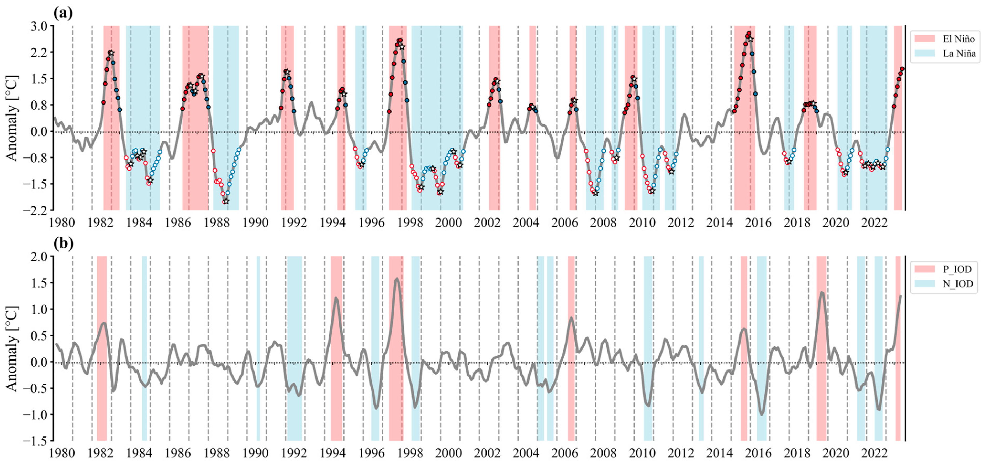
4.2. Selection of ENSO and IOD Events

We calculated the Ocean Niño Index (ONI) and Dipole Mode Index (DMI) using sea temperature from the Simple Ocean Data Assimilation version 3.15.2 (SODA3.15.2) dataset (Figure 2 and Figure S3). We defined the year in which the ENSO event occurred as the developing year and the following year as the decaying year [61]. We also adopted the ENSO phase division method proposed by Warner and Moum (2019) [62]. The ENSO developing years include El Niño warming and La Niña cooling, while the ENSO decaying years include El Niño cooling and La Niña warming.

These transitions include the transition to the fully perturbed (or peak) state of El Niño/La Niña and the relaxations back to the neutral state. We marked the transitions of these four phases with star-shaped dots (Figure 2a). When El Niño (or La Niña) reaches its peak, the inflection point of the gradient marks the phase transition. The months prior to this point are considered El Niño warming (or La Niña cooling), while the following months are considered El Niño cooling (or La Niña warming). Given that some ENSO events end in the same year or last for two to three years, we counted El Niño warming (or La Niña cooling) as the development phase of ENSO events and count El Niño cooling (or La Niña warming) as the decay phase (Figure 2a). Following this rule, we selected those years corresponding to the spring and fall branches in the ENSO decay and development phases, respectively (

Table 1. Years of the selected IOD and ENSO events (1980–2023).

Phase		Spring Wyrtki Jet	Fall Wyrtki Jet
ENSO developing	El Niño warming	–	1982, 1986, 1991, 1994, 1997, 2002, 2006, 2009, 2015, 2018, 2023
	La Niña cooling	–	1983, 1984, 1988, 1995, 1998, 1999, 2000, 2007, 2008, 2010, 2011, 2017, 2020, 2021, 2022
ENSO decaying	El Niño cooling	1983, 1987, 1992, 1998, 2016, 2019	–
	La Niña warming	1984, 1985, 1989, 1999, 2000, 2008, 2011, 2018, 2021, 2022	–
IOD	Positive IOD	1982, 1994, 1997	1982, 1994, 1997, 2006, 2015, 2019, 2023
	Neagtive IOD	1992, 2005, 2013, 2016	1984, 1992, 1996, 1998, 2005, 2010, 2016, 2021, 2022

).

We also selected those years corresponding to the spring and fall branches following the DMI phase definition. IOD shows seasonal phase-locking characteristics, that is, IOD events usually start to develop in June, reach their peak in October, and quickly disappear thereafter. We observed that in some years, positive IOD (pIOD) developed during spring, while negative IOD (nIOD) developed during spring and summer, before quickly disappearing (Figure 2b). We counted these phenomena in the years of the spring branch. Meanwhile, for IOD occurring in summer and fall, we screened out those years that coexist with the fall branch. Table 1 shows that the spring branch only appears in ENSO decaying phases, while the fall branch only appears in ENSO developing phases. IOD primarily occurs in the fall, resulting in fewer years being statistically accounted for in the spring branch compared to the fall branch.

4.3. General Description of Interannual WJ Variations

To highlight the common characteristics of WJs under the influence of interannual events, we conducted a composite analysis based on the selected years shown in Table 1. Given that WJs mainly occur during the monsoon transition period, the spring branch appears from the northeast to the southwest monsoon during the transition period (Figure 3a,b and Figure 4a,b). During the El Niño decaying phase, significant northeasterly wind stress anomalies are observed in the western Arabian Sea and the Bay of Bengal, while significant northwesterly wind stress anomalies are observed from 45° E to 100° E in the southern Indian Ocean. During this period, the monsoon region is abnormally weakened compared to its climatological state. At this time, the spring branch shows positive anomalies, and the significant areas are mainly located between 60° E and 80° E. During the La Niña decaying phase, the spring branch exhibits negative anomalies between 70° E and 100° E. At this time, significant southwesterly wind stress anomalies are observed over the Arabian Sea and the Bay of Bengal, while the southwestern Indian Ocean, between 40° E and 70° E, experiences notable southeasterly wind stress anomalies. Induced by the wind stress anomalies, the spring branch shows significant positive (negative) anomalies in the west (east) of the equatorial Indian Ocean in El Niño (La Niña) years. During the pIOD event, significant easterly wind stress anomalies occur near Sri Lanka, leading to negative anomalies in the spring branch. Meanwhile, during the nIOD event, significant northwesterly wind stress anomalies are observed near Sumatra, resulting in pronounced positive anomalies in the spring branch, mainly between 70° E and 100° E. The anomalies of the spring branch are more significant under nIOD than under pIOD.

The fall branch emerges during the transition from the southwest to the northeast monsoon (Figure 3c,d and Figure 4c,d). During the El Niño developing phase, it exhibits significant negative anomalies, accompanied by pronounced southeasterly wind stress anomalies near Sumatra. These anomalies extend eastward along the equator, where strong easterly wind stress anomalies reach the central Indian Ocean. Additionally, notable northeasterly wind stress anomalies are observed over the Bay of Bengal and the Arabian Sea. During the La Niña developing phase, the pattern is reversed. The fall branch also shows significant negative anomalies during pIOD events, with wind stress anomaly patterns resembling those observed during El Niño but with greater intensity. Conversely, during nIOD events, the fall branch exhibits significant positive anomalies, with wind stress anomalies opposite to those in pIOD events. The stronger positive feedback processes in the eastern Pacific during El Niño lead to greater temperature anomaly amplitudes compared to La Niña [63]. Furthermore, the skewness characteristics of IOD events result in a greater amplitude in pIOD events than in nIOD events [64]. Consequently, the anomaly intensity of the fall branch is more pronounced during El Niño and pIOD events than during La Niña and nIOD events.

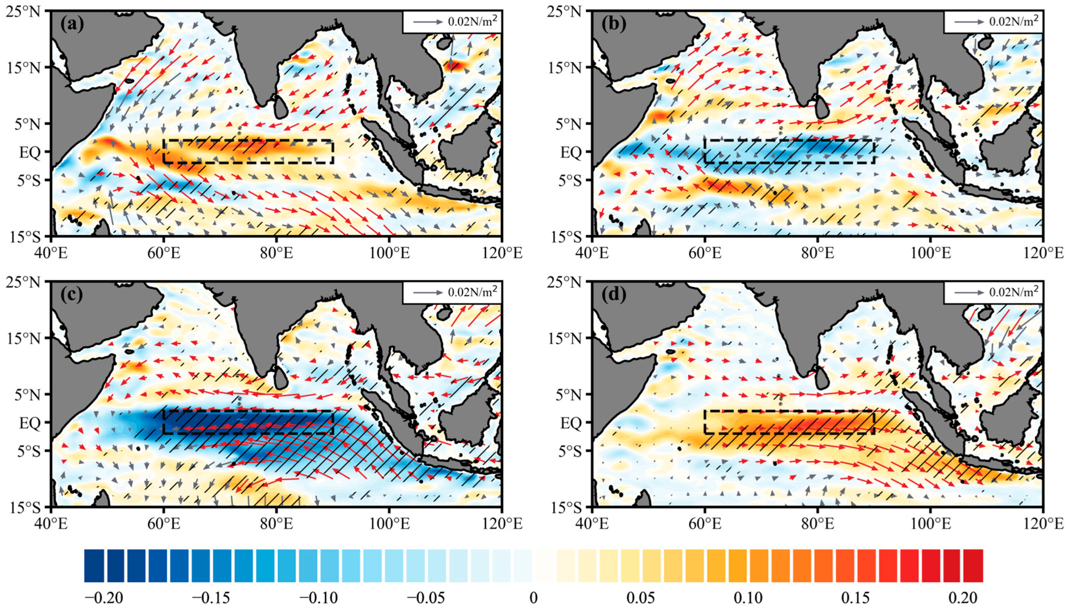
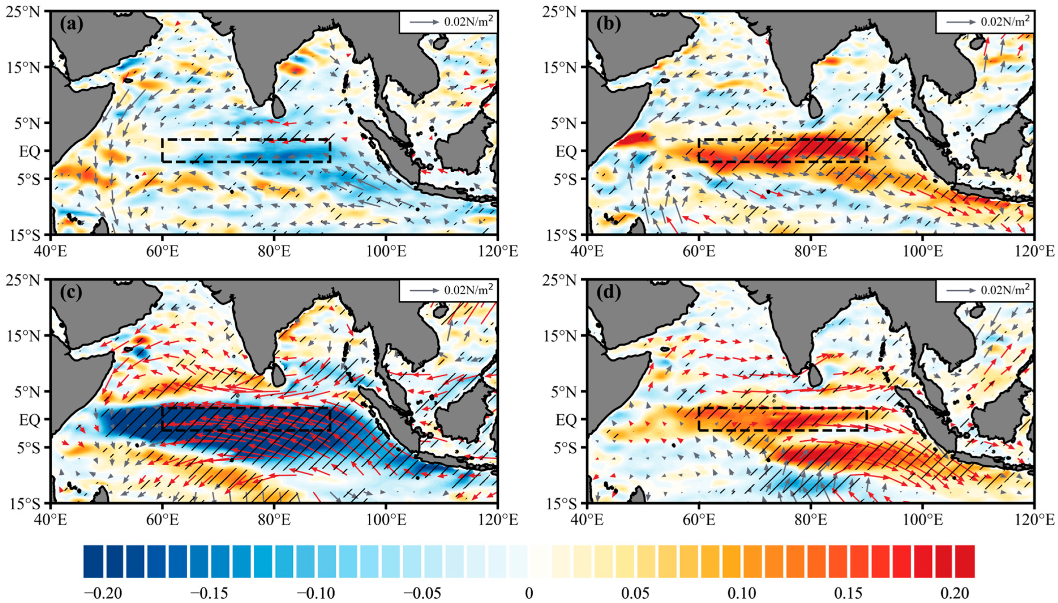
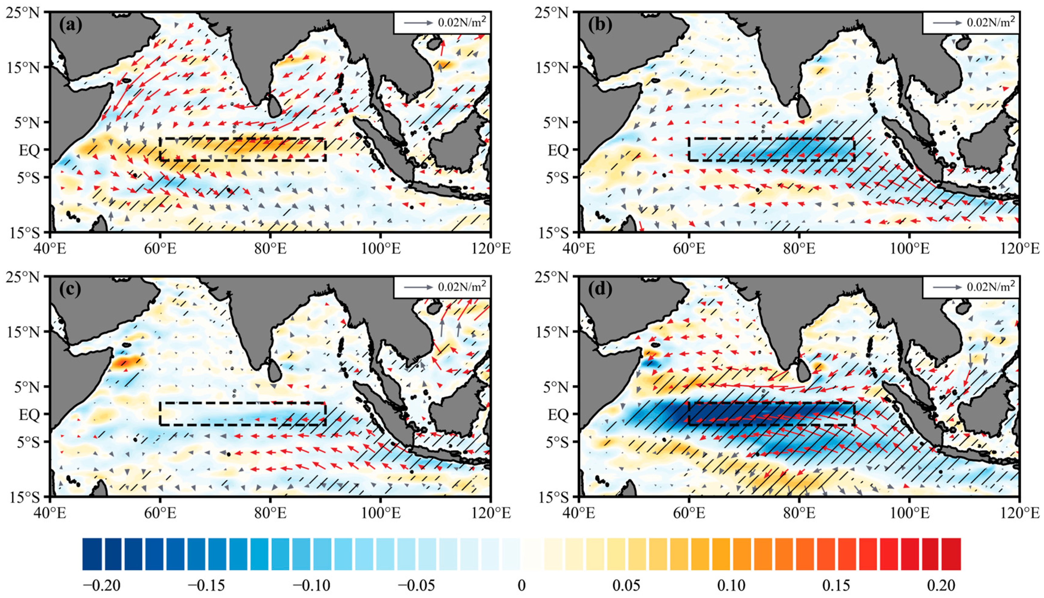
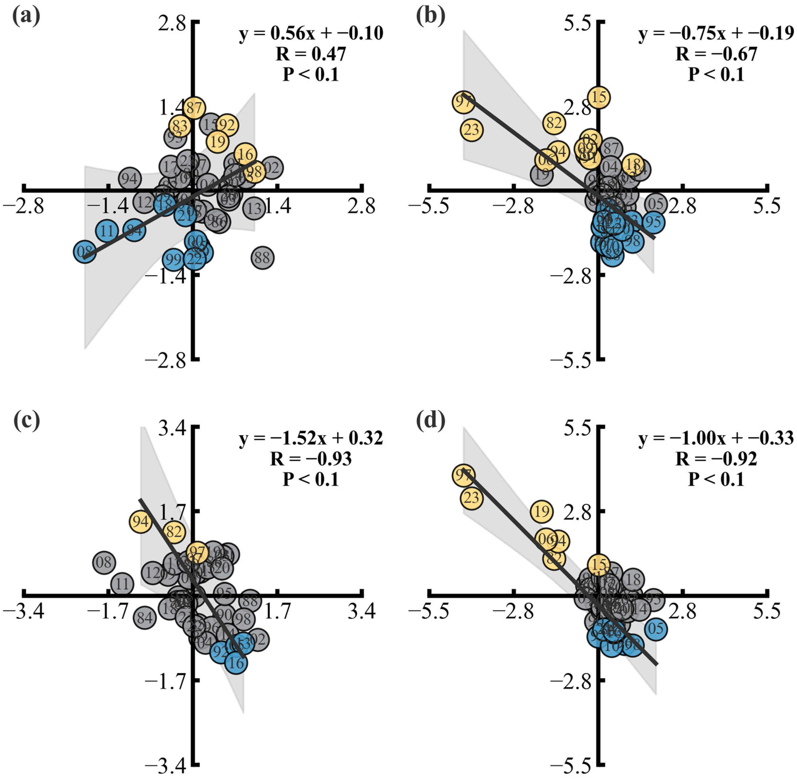
4.4. Influence of IOD and ENSO on WJ Variations

Given that ordinary composite and correlation analyses cannot easily distinguish the relationship between the spring and fall branches under the direct influence of ENSO or IOD, we calculated the partial correlation coefficients for the zonal current and wind stress anomalies using ONI and DMI, respectively, based on the screening year (Table 1) to clearly discern the independent correlation of these two branches in interannual events.

For the spring branch (Figure 5a,b), Figure 5a shows the partial correlation coefficients after removing the influence of IOD, revealing a significant positive correlation with the ENSO phase. During this period, wind stress anomalies over the Arabian Sea, the Bay of Bengal, and the southeastern Indian Ocean exhibit a strong correlation with ENSO. These regions fall within the monsoon domain, where the ENSO decaying phase influences the wind stress anomalies, thereby modulating the spring branch anomalies. Similarly, Figure 5b presents the partial correlation coefficients after removing the influence of ENSO, showing a significant negative correlation with the IOD phase. In this case, zonal wind anomalies from Sumatra to the western Indian Ocean are strongly associated with IOD, indicating that IOD-induced equatorial wind anomalies have a direct impact on the spring branch. The key factors driving the interannual variability of the spring branch are primarily linked to the ENSO decaying phase and IOD events. For the fall branch (Figure 5c,d), the ENSO and IOD events during fall both show significant negative correlations, with the negative correlation for IOD being stronger and the negative correlation for ENSO being weaker, both passing the 90% significance test. After removing the effect of IOD, the influence of the ENSO developing phase does not cover the whole equatorial Indian Ocean (Figure 5c,d) and is rather limited to the wind stress anomalies from the Sumatra–Java coast to 78° E, which modulate the fall branch anomalies. Similarly, after removing the influence of ENSO, the IOD events influence the wind stress anomalies along the Sumatra–Java coast, extending across the entire equatorial Indian Ocean. Meanwhile, wind anomalies over the Bay of Bengal and the Arabian Sea also contribute, collectively modulating the fall branch anomalies.

The phase-locking characteristics of ENSO influence the wind over the Indian Ocean through different causal pathways. During the developing phase of ENSO, anomalies in the Walker circulation play a crucial role. In El Niño events, the descending branch of the anomalous Walker circulation is positioned over the Maritime Continent and the tropical eastern Indian Ocean, triggering anomalous easterly winds from the tropical southeastern Indian Ocean toward the western Indian Ocean. Conversely, during La Niña events, the anomalous Walker circulation converges and ascends over the Maritime Continent and the tropical eastern Indian Ocean, while its descending branch shifts to the tropical western Indian Ocean, inducing anomalous westerly winds from the tropical western Indian Ocean toward the eastern Indian Ocean [32,65,66]. During the spring of the ENSO decaying phase, persistent large-scale convective anomalies are observed over the tropical northwestern Pacific and the northern Indian Ocean. As a response to the enhancement (suppression) of convective anomalies, Rossby wave dynamics induce significant easterly (westerly) vertical wind shear over the northern Indian Ocean. This vertical wind shear, in turn, exerts a substantial modulating effect on ISO activity through tropical wave dynamics, leading to enhanced (weakened) ISO activity over the Bay of Bengal following cold (warm) ENSO events. Consequently, the strengthened (weakened) northward-propagating ISO at the initial stage triggers an earlier (delayed) onset of the Bay of Bengal summer monsoon [67]. These findings further motivate us to explore the influence of ENSO and IOD on the zonal wind stress over the equatorial Indian Ocean, as well as the role of monsoon onset timing in regulating WJs.

Therefore, we further explored the roles of ENSO and IOD in modulating the zonal wind stresses in the WJs and the equatorial Indian Ocean. We constructed regression models for spring and fall based on the cases presented in Table. 1. Results show that building a single DMI or ONI model underestimates the strength of WJs and zonal wind stress; thus, using a multiple regression model is ideal (

Table 2. Explained variances R² of the single-regression ONI or DMI model and multiple regression on variables (τ_x and U) and their differences ∆ in regions 60° E–90° E in longitude and 2° S–2° N in latitude.

Model	Spring		Fall
	τx	U	τx	U
Multiple Regression Model	0.58	0.50	0.88	0.58
Single Regression Model (ONI)	0.26	0.14	0.54	0.38
∆	+0.32	+0.36	+0.30	+0.20
Single Regression Model (DMI)	0.34	0.32	0.86	0.55
∆	+0.24	+0.18	+0.02	+0.03

). The total explained variance of the spring model $U$ (${\tau }_x$) increased by 15% to 39% (25% to 34%) compared with those regression models that only consider IOD or ENSO, while the total explained variance of the fall model $U$ (${\tau }_x$) increased by 5% to 19% (3% to 34%). Based on these improvements in explained variance, we quantified the relative contribution of interannual events to the spring and fall branches by using a partial regression approach. The partial regression coefficients and partial correlation coefficients exhibit consistent patterns in their descriptions (Figure 6), where the partial regression coefficients represent the relative contribution of predictor factors to WJs anomalies and wind stress anomalies. Following the partial regression method in Wang et al. (2021) [58], we reconstructed the anomaly fields in the synthetic analysis by using partial regression coefficients and then separately analyzed the relative contributions of ENSO and IOD to the zonal current anomalies by using partial regression fields. During El Niño (La Niña) decaying years (Figures S4 and S5), the spatial modes of the reconstructed and original fields are almost the same, only with a few errors. Therefore, using partial regression fields to separately observe the contributions of ENSO and IOD to the spring branch can guarantee an excellent interpretability. During El Niño (La Niña) decaying years, the delayed (advanced) onset of the monsoon leads to positive (negative) anomalies in the spring branch. ENSO provides the primary contribution to the spring branch, with an anomaly contribution of +0.07 m/s (−0.05 m/s). In contrast, IOD contribution is weaker, with an anomaly contribution of +0.03 m/s (no contribution). The spatial modes of the reconstructed and pristine fields in the positive (negative) IOD years (Figures S6 and S7) are also the same, with the residual field being one order of magnitude less than the reconstructed field. The anomalies of the WJs are stronger in IOD than in ENSO. During IOD events, the WJs are primarily modulated by the IOD, with ENSO playing a weaker role. During positive (negative) IOD years, IOD provides the primary contribution to the spring branch, with an anomaly contribution of +0.15 m/s (−0.11 m/s). ENSO contribution is much weaker, with an anomaly contribution of +0.02 m/s (+0.03 m/s) in both cases.

ENSO and IOD trigger eastward (westward) wind stress anomalies in the equatorial Indian Ocean and suppress (enhance) the fall branch. During the El Niño (La Niña) developing years (Figures S8 and S9), the reconstruction field works well, with IOD provides the primary contribution to the fall branch, with an anomaly contribution of −0.11 m/s (+0.06 m/s), which is greater than ENSO anomaly contribution of −0.06 m/s (+0.04 m/s). The influence of IOD also extends to as far as 60° E, while that of ENSO only extends up to 80° E. During those years with a positive (negative) IOD (Figures S10 and S11), IOD provides the primary contribution to the fall branch, with an anomaly contribution of −0.2 m/s (+0.15 m/s), which is much larger than ENSO anomaly contribution of −0.07 m/s (+0.03 m/s).

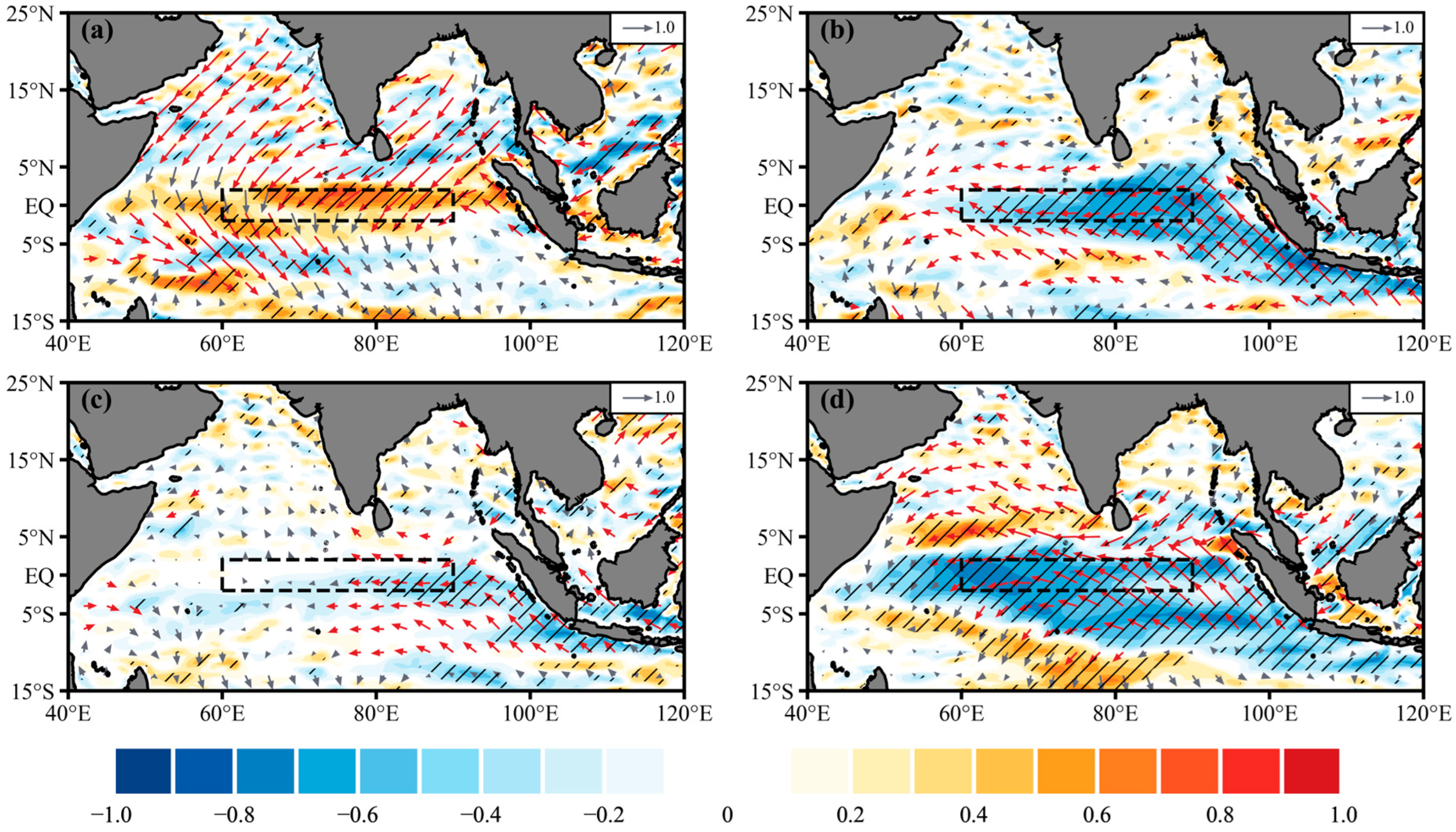
4.5. Regulatory Mechanisms of Abnormal WJs

We took the average of the WJs occurrence region and further determined the relationship of the spring and fall branches with interannual events (ENSO and IOD) through scatter relations. The spring branch exhibits positive (negative) anomalies during the El Niño (La Niña) decaying phase and shows a significant positive correlation (0.47) with the positive and negative phases of ENSO (Figure 7a). Meanwhile, under IOD events, the spring branch exhibits negative (positive) anomalies when positive (negative) IOD occurs and demonstrates a significant negative correlation (−0.93) with the positive and negative phases of IOD (Figure 7c). During the El Niño (La Niña) developing phase, the fall branch exhibits negative (positive) anomalies and a significant negative correlation (−0.68) with ENSO (Figure 7b). In positive (negative) IOD events, the fall branch exhibits a negative (positive) anomaly and a significant negative correlation (−0.92) with IOD (Figure 7d). The positive phase anomaly of the fall branch is notably stronger than its negative phase anomaly, primarily due to the greater amplitude of pIOD compared to nIOD. Given that WJs exist in the equatorial Indian Ocean and directly affect the east–west heat distribution, the correlation with IOD is more higher than that with ENSO.

Given that the responses of WJs are driven by zonal winds, we further explored the connection between zonal winds and interannual events. However, in analyzing the modulation of the spring branch by wind fields, we referred to the study by Li et al. (2022) [68], which found that the coordinated transition of equatorial westerlies and the southwest monsoon after monsoon onset plays a crucial role in regulating WJ intensity. A later (earlier) monsoon onset leads to a stronger (weaker) spring branch. Moreover, in the year following a cold (warm) ENSO event, convection over the northwestern Pacific is significantly enhanced (suppressed), creating favorable (unfavorable) conditions for the development of ISO over the Bay of Bengal. This, in turn, leads to an earlier (delayed) monsoon onset [67]. Based on this mechanism, we selected the monsoon regions of the Indian Ocean (the Bay of Bengal and the Arabian Sea) and the significantly affected areas in the southwestern Indian Ocean identified in the composite analysis. We then examined the zonal and meridional wind anomalies and marked interannual events with scatter points (Figure 8a–f). The wind anomalies reveal that during the decaying phase of El Niño (La Niña), both zonal and meridional winds in this region exhibit significant weakening (strengthening), indicating a delayed (advanced) monsoon onset. This delay (advance) in monsoon onset causes the transition of equatorial westerlies to lag (lead), resulting in a stronger (weaker) spring branch anomaly. As the primary driving force of surface currents in the Indian Ocean, the spring branch exhibits a pronounced response to the monsoon onset process. From Figure 8h, the spring zonal wind anomaly demonstrates a significant negative correlation (−0.83) with IOD events.

As the dominant mode of the ocean–atmosphere coupled system on interannual timescales, ENSO directly influences tropical atmospheric circulation. During the developing phase of ENSO, persistent zonal wind anomalies over the equatorial Pacific modulate the thermal contrast between the eastern and western Pacific. Through the Bjerknes positive feedback mechanism, these wind anomalies gradually amplify SSTAs while adjusting the intensity of the Walker circulation, ultimately inducing significant equatorial zonal wind anomalies over the Indian Ocean. To examine this effect, we selected the significant zonal wind region (80° E–100° E, 5° S–5° N) identified in Figure 5c. During the development of El Niño (La Niña), there is a clear suppression (enhancement) of westerly winds, leading to negative (positive) zonal wind anomalies (Figure 8g), showing a significant negative correlation (−0.84). Under the influence of strong interannual events, the zonal wind anomalies over the equator become more pronounced. When such anomalies occur, WJs exhibit corresponding anomalous signals, further confirming that their formation is driven by wind forcing. During IOD events (Figure 8i), equatorial wind anomalies show a significant negative correlation (−0.98) with the IOD phase, and the anomalous variations of WJs in both spring and fall exhibit a consistent pattern. This further verifies that wind anomalies induced by interannual events serve as the primary driver of WJ interannual variability.

5. Conclusions and Discussion

During the monsoon transition, WJs can cover the entire central equatorial Indian Ocean in the zonal direction, thus significantly affecting the east–west heat and salinity transport throughout the Indian Ocean [19,20,21]. When the El Niño decaying (La Niña developing) phase or the nIOD phase leads to the intensification of the spring (fall) branch, the anomalously strong eastward jet transports more warm water to the equatorial eastern Indian Ocean, significantly increasing the upper-ocean heat content in this region and creating favorable conditions for the enhancement of local atmospheric convection. These convective changes not only affect the local ecological environment and economic activities but also influence the monsoon system by modulating the Hadley circulation, thereby extending their impact across the entire East and South Asian monsoon regions. Conversely, when the La Niña decaying (El Niño developing) phase or the pIOD phase leads to the weakening of the spring (fall) branch, the positive thermal anomalies in the eastern Indian Ocean dissipate, leading to a corresponding reduction in their regulatory effect on local atmospheric circulation [14,50]. At the same time, when WJs reach the eastern boundary, they trigger Rossby waves that propagate downward and westward, affecting the strength of the Equatorial Undercurrent and playing a crucial role in regulating basin-scale material and energy distribution [69,70]. By affecting the sea-level anomalies on both sides of the Indian Ocean, it has a significant impact on the sea surface temperature changes and upwelling activities in the eastern Indian Ocean, making it have an important impact on the sea surface height, upper ocean heat content, sea surface temperature, salinity, and atmospheric convection activities in the equatorial Indian Ocean and even the northern Indian Ocean, making it a key regulatory factor in global climate variability [14,16,71].

In this study, we analyzed the interannual variability of WJs under the interactions of the Indo-Pacific ocean and the atmosphere along with their corresponding mechanisms by using ocean reanalysis data (SODA3.15.2) from 1980 to 2023. WJs are mainly active in the 60° E~90° E, 2° S~2° N region, reaching a peak intensity at 70° E~80° E and decaying from west to east. Its climatic state is that the spring branch is generally weaker than the fall branch. We selected the corresponding years through the four phases defined by Warner and Moum (2019) [62], and we filtered the spring and fall branches corresponding to the ENSO decaying and ENSO developing phases. We eventually identified the effects of ENSO and IOD on WJs via composite analysis and multiple regression, respectively.

Results show that ENSO regulates the interannual variability of the spring and fall branches of WJs through different mechanisms. Due to the seasonal phase-locking effect of ENSO, WJs exhibit distinct response characteristics: the spring branch shows positive (negative) anomalies during the El Niño (La Niña) decaying phases, while the fall branch exhibits negative (positive) anomalies during the El Niño (La Niña) developing phases. Meanwhile, IOD directly drives equatorial wind anomalies through local air–sea feedback, with positive (negative) IOD events leading to negative (positive) anomalies in both the spring and fall branches. The stronger amplitude of positive IOD events results in more pronounced anomalies in the fall branch. We used partial correlation to separate the relationship between ENSO and IOD, and results show that the spring branch has a significant positive correlation with ENSO and a significant negative correlation with IOD. For the fall branch, both ENSO and IOD exhibit significant negative correlations. The variance explained by the combined influence of ENSO and IOD on WJs is significantly higher than that of either factor alone. Multiple regression models indicate that ENSO is the primary driver of interannual variability in the spring branch, while IOD is the dominant factor for the fall branch. The mechanisms underlying interannual anomalies differ between the spring and fall branches. For the spring branch, ENSO regulates its intensity indirectly by influencing monsoon onset timing: in El Niño (La Niña) decaying years, delayed (advanced) monsoon onset leads to a lagged (advanced) shift in equatorial westerlies, thereby strengthening (weakening) the spring branch. In contrast, for the fall branch, ENSO modulates zonal currents by altering the position of the descending branch of the Walker circulation, but its impact is relatively limited, primarily affecting the central equatorial Indian Ocean. In comparison, IOD influences WJs by inducing anomalous zonal winds across the entire equatorial Indian Ocean through its basin-wide mechanisms.

This study focuses on characterizing the interannual response of WJs and their regulation mechanisms under the interactions between the Indo-Pacific ocean and the atmosphere. Previous studies have suggested that the interannual variability of the spring branch is primarily controlled by intraseasonal wind variations and cannot be explained by interannual forcing events such as ENSO and IOD [50,72]. However, our findings demonstrate that the spring branch exhibits significant interannual variability, primarily regulated by ENSO through its influence on monsoon onset timing, which indirectly modulates the spring branch [67,68]. Due to the influence of intraseasonal effects and the limitations of data temporal resolution, the direct modulation of spring branch interannual characteristics by equatorial zonal wind anomalies cannot be accurately captured. Therefore, understanding the role of the spring branch and its low-frequency variability in the Indian Ocean dipole zonal model [41], monsoon variability, and ENSO–monsoon interactions should be further explored [66,73,74]. The mechanism of ENSO–monsoon interactions on the interannual variability of WJs in this study also warrants further investigation.

In the context of global warming, the frequency and intensity of El Niño events may increase [75,76], decrease [77], or depend on changes in the mean climate state [78]. Accordingly, ENSO characteristics may also change in the future [79], which subsequently changes the interannual characteristics of WJs. ENSO plays a key role not only in the occurrence and development of IOD [80] but also in the interannual variability of WJs. Therefore, the feedback mechanisms of the Indo-Pacific interannual events on WJs should be systematically investigated to enhance the current understanding of ocean dynamics, ecosystems, and climate effects in the tropical Indian Ocean.

References

1. Schott, F.A.; McCreary, J.P. The Monsoon Circulation of the Indian Ocean. Prog. Oceanogr. 2001, 51, 1–123. [Google Scholar] [CrossRef]
2. Schott, F.A.; Xie, S.-P.; McCreary, J.P., Jr. Indian Ocean Circulation and Climate Variability. Rev. Geophys. 2009, 47, RG1002. [Google Scholar] [CrossRef]
3. Wyrtki, K. An Equatorial Jet in the Indian Ocean. Science 1973, 181, 262–264. [Google Scholar] [CrossRef]
4. Molinari, R.L.; Olson, D.; Reverdin, G. Surface Current Distributions in the Tropical Indian Ocean Derived from Compilations of Surface Buoy Trajectories. J. Geophys. Res. Ocean. 1990, 95, 7217–7238. [Google Scholar] [CrossRef]
5. Reppin, J.; Schott, F.A.; Fischer, J.; Quadfasel, D. Equatorial Currents and Transports in the Upper Central Indian Ocean: Annual Cycle and Interannual Variability. J. Geophys. Res. Ocean. 1999, 104, 15495–15514. [Google Scholar] [CrossRef]
6. Yuan, D.; Han, W. Roles of Equatorial Waves and Western Boundary Reflection in the Seasonal Circulation of the Equatorial Indian Ocean. J. Phys. Oceanogr. 2006, 36, 930–944. [Google Scholar] [CrossRef]
7. O’Brien, J.J.; Hurlburt, H.E. Equatorial Jet in the Indian Ocean: Theory. Science 1974, 184, 1075–1077. [Google Scholar] [CrossRef]
8. Nagura, M.; McPhaden, M.J. Wyrtki Jet Dynamics: Seasonal Variability. J. Geophys. Res. Ocean. 2010, 115. [Google Scholar] [CrossRef]
9. Han, W.; McCreary, J.P.; Anderson, D.L.T.; Mariano, A.J. Dynamics of the Eastern Surface Jets in the Equatorial Indian Ocean. J. Phys. Oceanogr. 1999, 29, 2191–2209. [Google Scholar] [CrossRef]
10. Qiu, Y.; Li, L.; Yu, W. Behavior of the Wyrtki Jet Observed with Surface Drifting Buoys and Satellite Altimeter. Geophys. Res. Lett. 2009, 36, L18607. [Google Scholar] [CrossRef]
11. Jensen, T.G. Equatorial Variability and Resonance in a Wind-Driven Indian Ocean Model. J. Geophys. Res. Ocean. 1993, 98, 22533–22552. [Google Scholar] [CrossRef]
12. McPhaden, M.J.; Wang, Y.; Ravichandran, M. Volume Transports of the Wyrtki Jets and Their Relationship to the Indian Ocean Dipole. J. Geophys. Res. Ocean. 2015, 120, 5302–5317. [Google Scholar] [CrossRef]
13. Duan, Y.; Liu, L.; Han, G.; Liu, H.; Yu, W.; Yang, G.; Wang, H.; Wang, H.; Liu, Y.; Zahid; et al. Anomalous Behaviors of Wyrtki Jets in the Equatorial Indian Ocean during 2013. Sci. Rep. 2016, 6, 29688. [Google Scholar] [CrossRef]
14. Cao, G.; Xu, T.; Wei, Z. Research progress on intraseasonal variability of Wyrtki jet. Prog. Geophys. 2024, 39, 1293–1303. [Google Scholar] [CrossRef]
15. Shinoda, T.; Han, W.; Metzger, E.J.; Hurlburt, H.E. Seasonal Variation of the Indonesian Throughflow in Makassar Strait. J. Phys. Oceanogr. 2012, 42, 1099–1123. [Google Scholar] [CrossRef]
16. Cao, G.; Xu, T.; Wei, Z. Seasonal Differences of Wyrtki Jet Intraseasonal Variabilities. Front. Mar. Sci. 2024, 11, 1517779. [Google Scholar] [CrossRef]
17. Zhang, Y.; Du, Y. Seasonal Variability of Salinity Budget and Water Exchange in the Northern Indian Ocean from HYCOM Assimilation. Chin. J. Ocean. Limnol. 2012, 30, 1082–1092. [Google Scholar] [CrossRef]
18. Zhang, Y.; Du, Y.; Zheng, S.; Yang, Y.; Cheng, X. Impact of Indian Ocean Dipole on the Salinity Budget in the Equatorial Indian Ocean. J. Geophys. Res. Ocean. 2013, 118, 4911–4923. [Google Scholar] [CrossRef]
19. Zhang, Y.; Du, Y.; Zhang, Y.; Gao, S. Asymmetry of Upper Ocean Salinity Response to the Indian Ocean Dipole Events as Seen from ECCO Simulation. Acta Oceanol. Sin. 2016, 35, 42–49. [Google Scholar] [CrossRef]
20. Wang, J. Observational Bifurcation of Wyrtki Jets and Its Influence on the Salinity Balance in the Eastern Indian Ocean. Atmos. Ocean. Sci. Lett. 2017, 10, 36–43. [Google Scholar]
21. Xie, C.; Ding, R.; Xuan, J.; Huang, D. Interannual Variations in Salt Flux at 80°E Section of the Equatorial Indian Ocean. Sci. China Earth Sci. 2023, 66, 2142–2161. [Google Scholar] [CrossRef]
22. Murtugudde, R.; McCreary, J.P., Jr.; Busalacchi, A.J. Oceanic Processes Associated with Anomalous Events in the Indian Ocean with Relevance to 1997–1998. J. Geophys. Res. Ocean. 2000, 105, 3295–3306. [Google Scholar] [CrossRef]
23. Masson, S.; Delecluse, P.; Boulanger, J.-P.; Menkes, C. A Model Study of the Seasonal Variability and Formation Mechanisms of the Barrier Layer in the Eastern Equatorial Indian Ocean. J. Geophys. Res. Ocean. 2002, 107, SRF-18-1–SRF 18-20. [Google Scholar] [CrossRef]
24. McPhaden, M.J.; Zebiak, S.E.; Glantz, M.H. ENSO as an Integrating Concept in Earth Science. Science 2006, 314, 1740–1745. [Google Scholar] [CrossRef]
25. Guan, C.; Chen, Y.; Wang, F. Seasonal Variability of Zonal Heat Advection in the Mixed Layer of the Tropical Pacific. Chin. J. Ocean. Limnol. 2013, 31, 1356–1367. [Google Scholar] [CrossRef]
26. Guan, C.; Hu, S.; McPhaden, M.J.; Wang, F.; Gao, S.; Hou, Y. Dipole Structure of Mixed Layer Salinity in Response to El Niño-La Niña Asymmetry in the Tropical Pacific. Geophys. Res. Lett. 2019, 46, 12165–12172. [Google Scholar] [CrossRef]
27. Saji, N.H.; Goswami, B.N.; Vinayachandran, P.N.; Yamagata, T. A Dipole Mode in the Tropical Indian Ocean. Nature 1999, 401, 360–363. [Google Scholar] [CrossRef]
28. Chowdary, J.S.; Gnanaseelan, C. Basin-Wide Warming of the Indian Ocean during El Niño and Indian Ocean Dipole Years. Int. J. Climatol. 2007, 27, 1421–1438. [Google Scholar] [CrossRef]
29. Webster, P.J.; Moore, A.M.; Loschnigg, J.P.; Leben, R.R. Coupled Ocean–Atmosphere Dynamics in the Indian Ocean during 1997–1998. Nature 1999, 401, 356–360. [Google Scholar] [CrossRef]
30. Feng, M.; Meyers, G.; Wijffels, S. Interannual Upper Ocean Variability in the Tropical Indian Ocean. Geophys. Res. Lett. 2001, 28, 4151–4154. [Google Scholar] [CrossRef]
31. Rao, S.A.; Behera, S.K.; Masumoto, Y.; Yamagata, T. Interannual Subsurface Variability in the Tropical Indian Ocean with a Special Emphasis on the Indian Ocean Dipole. Deep. Sea Res. Part. II Top. Stud. Oceanogr. 2002, 49, 1549–1572. [Google Scholar] [CrossRef]
32. Saji, N.H.; Yamagata, T. Possible Impacts of Indian Ocean Dipole Mode Events on Global Climate. Clim. Res. 2003, 25, 151–169. [Google Scholar] [CrossRef]
33. Feng, M.; Meyers, G. Interannual Variability in the Tropical Indian Ocean: A Two-Year Time-Scale of Indian Ocean Dipole. Deep. Sea Res. Part. II Top. Stud. Oceanogr. 2003, 50, 2263–2284. [Google Scholar] [CrossRef]
34. McPhaden, M.J.; Nagura, M. Indian Ocean Dipole Interpreted in Terms of Recharge Oscillator Theory. Clim. Dyn. 2014, 42, 1569–1586. [Google Scholar] [CrossRef]
35. Nyadjro, E.S.; McPhaden, M.J. Variability of Zonal Currents in the Eastern Equatorial Indian Ocean on Seasonal to Interannual Time Scales. J. Geophys. Res. Ocean. 2014, 119, 7969–7986. [Google Scholar] [CrossRef]
36. Yuan, D.; Liu, H. Long-Wave Dynamics of Sea Level Variations during Indian Ocean Dipole Events. J. Phys. Oceanogr. 2009, 39, 1115–1132. [Google Scholar] [CrossRef]
37. Chambers, D.P.; Tapley, B.D.; Stewart, R.H. Anomalous Warming in the Indian Ocean Coincident with El Niño. J. Geophys. Res. Ocean. 1999, 104, 3035–3047. [Google Scholar] [CrossRef]
38. Le Blanc, J.-L.; Boulanger, J.-P. Propagation and Reflection of Long Equatorial Waves in the Indian Ocean from TOPEX/POSEIDON Data during the 1993–1998 Period. Clim. Dyn. 2001, 17, 547–557. [Google Scholar] [CrossRef]
39. Huang, B.; Kinter III, J.L. Interannual Variability in the Tropical Indian Ocean. J. Geophys. Res. Ocean. 2002, 107, 20-1–20-26. [Google Scholar] [CrossRef]
40. Gnanaseelan, C.; Deshpande, A.; McPhaden, M.J. Impact of Indian Ocean Dipole and El Niño/Southern Oscillation Wind-Forcing on the Wyrtki Jets. J. Geophys. Res. Ocean. 2012, 117, C8. [Google Scholar] [CrossRef]
41. Joseph, S.; Wallcraft, A.J.; Jensen, T.G.; Ravichandran, M.; Shenoi, S.S.C.; Nayak, S. Weakening of Spring Wyrtki Jets in the Indian Ocean during 2006–2011. J. Geophys. Res. Ocean. 2012, 117, C4. [Google Scholar] [CrossRef]
42. Wu, Y.; Liu, L.; Zhang, X.; Duan, Y.; Yang, G.; Yang, Y.; Zahid; Oloo, P.; Sagero, P. Different Impacts from Various El Niño Events on Wyrtki Jets in Boreal Autumn Season. Pure Appl. Geophys. 2018, 175, 4567–4577. [Google Scholar] [CrossRef]
43. Deng, K.; Cheng, X.; Feng, T.; Ma, T.; Duan, W.; Chen, J. Interannual Variability of the Spring Wyrtki Jet. J. Ocean. Limnol. 2021, 39, 26–44. [Google Scholar] [CrossRef]
44. Chu, X.; Han, W.; Zhang, L.; Chen, G. Effects of Climate Modes on Interannual Variability of the Equatorial Currents in the Indian Ocean. Clim. Dyn. 2023, 60, 3681–3694. [Google Scholar] [CrossRef]
45. Ueda, H.; Matsumoto, J. A Possible Triggering Process of East-West Asymmetric Anomalies over the Indian Ocean in Relation to 1997/98 El Niño. J. Meteorol. Soc. Japan. Ser. II 2000, 78, 803–818. [Google Scholar] [CrossRef]
46. Hendon, H.H. Indonesian Rainfall Variability: Impacts of ENSO and Local Air–Sea Interaction. J. Clim. 2003, 16, 1775–1790. [Google Scholar] [CrossRef]
47. Lau, N.-C.; Nath, M.J. Atmosphere–Ocean Variations in the Indo-Pacific Sector during ENSO Episodes. J. Clim. 2003, 16, 3–20. [Google Scholar] [CrossRef]
48. Tokinaga, H.; Tanimoto, Y. Seasonal Transition of SST Anomalies in the Tropical Indian Ocean during El Niño and Indian Ocean Dipole Years. J. Meteorol. Soc. Japan. Ser. II 2004, 82, 1007–1018. [Google Scholar] [CrossRef]
49. Wang, B.; Wu, R.; Li, T. Atmosphere–Warm Ocean Interaction and Its Impacts on Asian–Australian Monsoon Variation. J. Clim. 2003, 16, 1195–1211. [Google Scholar] [CrossRef]
50. Deshpande, A.; Gnanaseelan, C.; Chowdary, J.S.; Rahul, S. Interannual Spring Wyrtki Jet Variability and Its Regional Impacts. Dyn. Atmos. Ocean. 2017, 78, 26–37. [Google Scholar] [CrossRef]
51. Gnanaseelan, C.; Deshpande, A. Equatorial Indian Ocean Subsurface Current Variability in an Ocean General Circulation Model. Clim. Dyn. 2018, 50, 1705–1717. [Google Scholar] [CrossRef]
52. Zhang, Y.; Guan, Y.P.; Huang, R.X. 3D Structure of Striations in the North Pacific. J. Phys. Oceanogr. 2021, 51, 3651–3662. [Google Scholar] [CrossRef]
53. Carton, J.A.; Chepurin, G.A.; Chen, L. SODA3: A New Ocean Climate Reanalysis. J. Clim. 2018, 31, 6967–6983. [Google Scholar] [CrossRef]
54. Naseef, T.M.; Kumar, V.S. Climatology and Trends of the Indian Ocean Surface Waves Based on 39-Year Long ERA5 Reanalysis Data. Int. J. Climatol. 2020, 40, 979–1006. [Google Scholar] [CrossRef]
55. McPhaden, M.J.; Meyers, G.; Ando, K.; Masumoto, Y.; Murty, V.S.N.; Ravichandran, M.; Syamsudin, F.; Vialard, J.; Yu, L.; Yu, W. RAMA: The Research Moored Array for African–Asian–Australian Monsoon Analysis and Prediction*. Bull. Am. Meteorol. Soc. 2009, 90, 459–480. [Google Scholar] [CrossRef]
56. Cai, W.; van Rensch, P.; Cowan, T.; Hendon, H.H. Teleconnection Pathways of ENSO and the IOD and the Mechanisms for Impacts on Australian Rainfall. J. Clim. 2011, 24, 3910–3923. [Google Scholar] [CrossRef]
57. Ham, Y.-G.; Kug, J.-S.; Park, J.-Y. Two Distinct Roles of Atlantic SSTs in ENSO Variability: North Tropical Atlantic SST and Atlantic Niño. Geophys. Res. Lett. 2013, 40, 4012–4017. [Google Scholar] [CrossRef]
58. Wang, J.-Z.; Wang, C. Joint Boost to Super El Niño from the Indian and Atlantic Oceans. J. Clim. 2021, 34, 4937–4954. [Google Scholar] [CrossRef]
59. Ashok, K.; Behera, S.K.; Rao, S.A.; Weng, H.; Yamagata, T. El Niño Modoki and Its Possible Teleconnection. J. Geophys. Res. 2007, 112, C11007. [Google Scholar] [CrossRef]
60. Hastenrath, S.; Greischar, L. The Monsoonal Current Regimes of the Tropical Indian Ocean: Observed Surface Flow Fields and Their Geostrophic and Wind-Driven Components. J. Geophys. Res. Ocean. 1991, 96, 12619–12633. [Google Scholar] [CrossRef]
61. Rasmusson, E.M.; Carpenter, T.H. Variations in Tropical Sea Surface Temperature and Surface Wind Fields Associated with the Southern Oscillation/El Niño. Mon. Weather. Rev. 1982, 110, 354–384. [Google Scholar] [CrossRef]
62. Warner, S.J.; Moum, J.N. Feedback of Mixing to ENSO Phase Change. Geophys. Res. Lett. 2019, 46, 13920–13927. [Google Scholar] [CrossRef]
63. Guan, C.; McPhaden, M.J.; Wang, F.; Hu, S. Quantifying the Role of Oceanic Feedbacks on ENSO Asymmetry. Geophys. Res. Lett. 2019, 46, 2140–2148. [Google Scholar] [CrossRef]
64. Cai, W.; Zheng, X.-T.; Weller, E.; Collins, M.; Cowan, T.; Lengaigne, M.; Yu, W.; Yamagata, T. Projected Response of the Indian Ocean Dipole to Greenhouse Warming. Nat. Geosci. 2013, 6, 999–1007. [Google Scholar] [CrossRef]
65. Krishnamurthy, V.; Kirtman, B.P. Variability of the Indian Ocean: Relation to Monsoon and ENSO. Q. J. R. Meteorol. Soc. 2003, 129, 1623–1646. [Google Scholar] [CrossRef]
66. Annamalai, H.; Xie, S.P.; McCreary, J.P.; Murtugudde, R. Impact of Indian Ocean Sea Surface Temperature on Developing El Niño. J. Clim. 2005, 18, 302–319. [Google Scholar] [CrossRef]
67. Li, K.; Liu, Y.; Li, Z.; Yang, Y.; Feng, L.; Khokiattiwong, S.; Yu, W.; Liu, S. Impacts of ENSO on the Bay of Bengal Summer Monsoon Onset via Modulating the Intraseasonal Oscillation. Geophys. Res. Lett. 2018, 45, 5220–5228. [Google Scholar] [CrossRef]
68. Li, K.; Yin, Y.; Yang, Y.; Liu, Y.; Yu, W. Dynamic Response of the Spring Wyrtki Jet to the Monsoon Onset Over the Bay of Bengal. Geophys. Res. Lett. 2022, 49, e2022GL101435. [Google Scholar] [CrossRef]
69. Huang, K.; Wang, D.; Chen, G.; Nagura, M.; Han, W.; McPhaden, M.J.; Feng, M.; Chen, J.; Wu, Y.; Zhang, X.; et al. Intensification and Dynamics of the Westward Equatorial Undercurrent During the Summers of 1998 and 2016 in the Indian Ocean. Geophys. Res. Lett. 2022, 49, e2022GL100168. [Google Scholar] [CrossRef]
70. Srinivas, G.; Amol, P.; Mukherjee, A. Influence of the Extreme Indian Ocean Dipole 2019 on the Equatorial Indian Ocean Circulation. Clim Dyn 2024, 62, 7111–7125. [Google Scholar] [CrossRef]
71. Masumoto, Y.; Hase, H.; Kuroda, Y.; Matsuura, H.; Takeuchi, K. Intraseasonal Variability in the Upper Layer Currents Observed in the Eastern Equatorial Indian Ocean. Geophys. Res. Lett. 2005, 32, 2. [Google Scholar] [CrossRef]
72. Prerna, S.; Chatterjee, A.; Mukherjee, A.; Ravichandran, M.; Shenoi, S.S.C. Wyrtki Jets: Role of Intraseasonal Forcing. J. Earth Syst. Sci. 2019, 128, 21. [Google Scholar] [CrossRef]
73. Wu, R.; Kirtman, B.P. Impacts of the Indian Ocean on the Indian Summer Monsoon–ENSO Relationship. J. Clim. 2004, 17, 3037–3054. [Google Scholar] [CrossRef]
74. Krishnan, R.; Ayantika, D.C.; Kumar, V.; Pokhrel, S. The Long-Lived Monsoon Depressions of 2006 and Their Linkage with the Indian Ocean Dipole. Int. J. Climatol. 2011, 31, 1334–1352. [Google Scholar] [CrossRef]
75. Roeckner, E.; Oberhuber, J.M.; Bacher, A.; Christoph, M.; Kirchner, I. ENSO Variability and Atmospheric Response in a Global Coupled Atmosphere-Ocean GCM. Clim. Dyn. 1996, 12, 737–754. [Google Scholar] [CrossRef]
76. Cai, W.; Borlace, S.; Lengaigne, M.; van Rensch, P.; Collins, M.; Vecchi, G.; Timmermann, A.; Santoso, A.; McPhaden, M.J.; Wu, L.; et al. Increasing Frequency of Extreme El Niño Events Due to Greenhouse Warming. Nat. Clim. Change 2014, 4, 111–116. [Google Scholar] [CrossRef]
77. Marjani, S.; Alizadeh-Choobari, O.; Irannejad, P. Frequency of Extreme El Niño and La Niña Events under Global Warming. Clim. Dyn. 2019, 53, 5799–5813. [Google Scholar] [CrossRef]
78. Wang, B.; Luo, X.; Yang, Y.-M.; Sun, W.; Cane, M.A.; Cai, W.; Yeh, S.-W.; Liu, J. Historical Change of El Niño Properties Sheds Light on Future Changes of Extreme El Niño. Proc. Natl. Acad. Sci. 2019, 116, 22512–22517. [Google Scholar] [CrossRef]
79. Yang, S.; Li, Z.; Yu, J.-Y.; Hu, X.; Dong, W.; He, S. El Niño–Southern Oscillation and Its Impact in the Changing Climate. Natl. Sci. Rev. 2018, 5, 840–857. [Google Scholar] [CrossRef]
80. Stuecker, M.F.; Timmermann, A.; Jin, F.-F.; Chikamoto, Y.; Zhang, W.; Wittenberg, A.T.; Widiasih, E.; Zhao, S. Revisiting ENSO/Indian Ocean Dipole Phase Relationships. Geophys. Res. Lett. 2017, 44, 2481–2492. [Google Scholar] [CrossRef]
Figure 1. Spatiotemporal distribution of zonal currents in the upper layer of the equatorial Indian Ocean (shading; units: m/s). (a) The temporal evolution of zonal currents; and (b,c) the zonal current (upper 15 m) distribution after meridional averaging (from 2° N to 2° S) in spring (April–May) and fall (October–November), respectively.
Jmse 13 00691 g001
Figure 2. (a) ONI, where the shaded area indicates that the SSTAs exceeds ±0.5 °C for more than five consecutive months, the light red shade represents the El Niño event, and the light blue shade represents the La Niña event. The red dots correspond to the developing phase of the ENSO events (El Niño warming or La Niña cooling), the blue dots correspond to the decaying phase of the ENSO events (El Niño cooling or La Niña warming), and the white star-shaped dots represent the phase transition of the event. (b) DMI, where the light red and light blue shades represent pIOD and nIOD events, respectively, and the judgment criterion is that the SSTAs exceeds ±0.4 °C for more than three consecutive months.
Jmse 13 00691 g002
Figure 3. Composite analysis of zonal current anomalies (shading, units: m/s) and wind stress anomalies (vectors, units: N/m²) in ENSO years. (a,b) Decaying stage of El Niño/La Niña for spring branch; (c,d) developing stage of El Niño/La Niña for fall branch. Black dotted box marks jet area, while red arrows and oblique lines indicate significant zonal wind stress and zonal current (90% significance, student’s t-test).
Jmse 13 00691 g003
Figure 4. Composite analysis of zonal current anomalies (shading, units: m/s) and wind stress anomalies (vectors, units: N/m²) in IOD years, (a,b) refer to the spring branch of WJs, where (a,b) are the composites for years with pIOD and nIOD, respectively; and (c,d) refer to the fall branch of WJs, where (c,d) are the composites for years with pIOD and nIOD, respectively.
Jmse 13 00691 g004
Figure 5. The spatial distribution of the partial correlation coefficients of the zonal current anomalies (shading, correlation) and wind stress anomalies (vectors, correlation) based on ONI and DMI. (a,b) represent the spring branch: (a) R s p r i n g O N I | D M I and (b) R s p r i n g D M I | O N I ; (c,d) represent the fall branch: (c) R f a l l O N I | D M I and (d) R f a l l D M I | O N I .
Jmse 13 00691 g005
Figure 6. Spatial distribution of the partial regression coefficient zonal current anomalies (shading, units: m/s) and wind stress anomalies (vectors, units: N/m2). (a,b) represent the spring branch: (a) a s p r i n g O N I | D M I and (b) b s p r i n g D M I | O N I ; (c,d) represent the fall branch: (c) a f a l l O N I | D M I and (d) b f a l l D M I | O N I . The 90% significance test markings follow the same convention as in Figure 3 but are based on the F-test.
Jmse 13 00691 g006
Figure 7. Scatter plots of zonal current anomalies (60° E–90° E, 2° S–2° N, upper 15 m of the equatorial Indian Ocean) versus ONI and DMI. (a,c) show the spring branch anomaly versus ENSO and IOD, respectively; and (b,d) refer to the corresponding anomalies for the fall branch. Those years with positive and negative phases are marked in yellow and blue, respectively.
Jmse 13 00691 g007
Figure 8. Scatter plots of wind anomalies. (ac) show the zonal wind anomalies in the Bay of Bengal (80° E–100° E, 2° N–15° N), the Arabian Sea (40° E–80° E, 2° N–15° N), and the southwestern Indian Ocean (40° E–80° E, 2° S–12° S), respectively. (df) represent the meridional wind anomalies in the same regions as (ac) during spring. (g) shows the zonal wind anomalies over the equatorial eastern Indian Ocean (80° E–100° E, 5° S–5° N) during fall. (h,i) depict the zonal wind anomalies over the equatorial Indian Ocean (40° E–100° E, 5° S–5° N) during spring and fall, respectively. Those years with positive and negative phases are marked in yellow and blue, respectively.
Jmse 13 00691 g008