

Analysis, Forecasting, and System Identification of a Floating Offshore Wind Turbine Using Dynamic Mode Decomposition

 ,
,  , , ,
, , ,  ,
,  and
and
Abstract
1. Introduction
2. Material and Methods
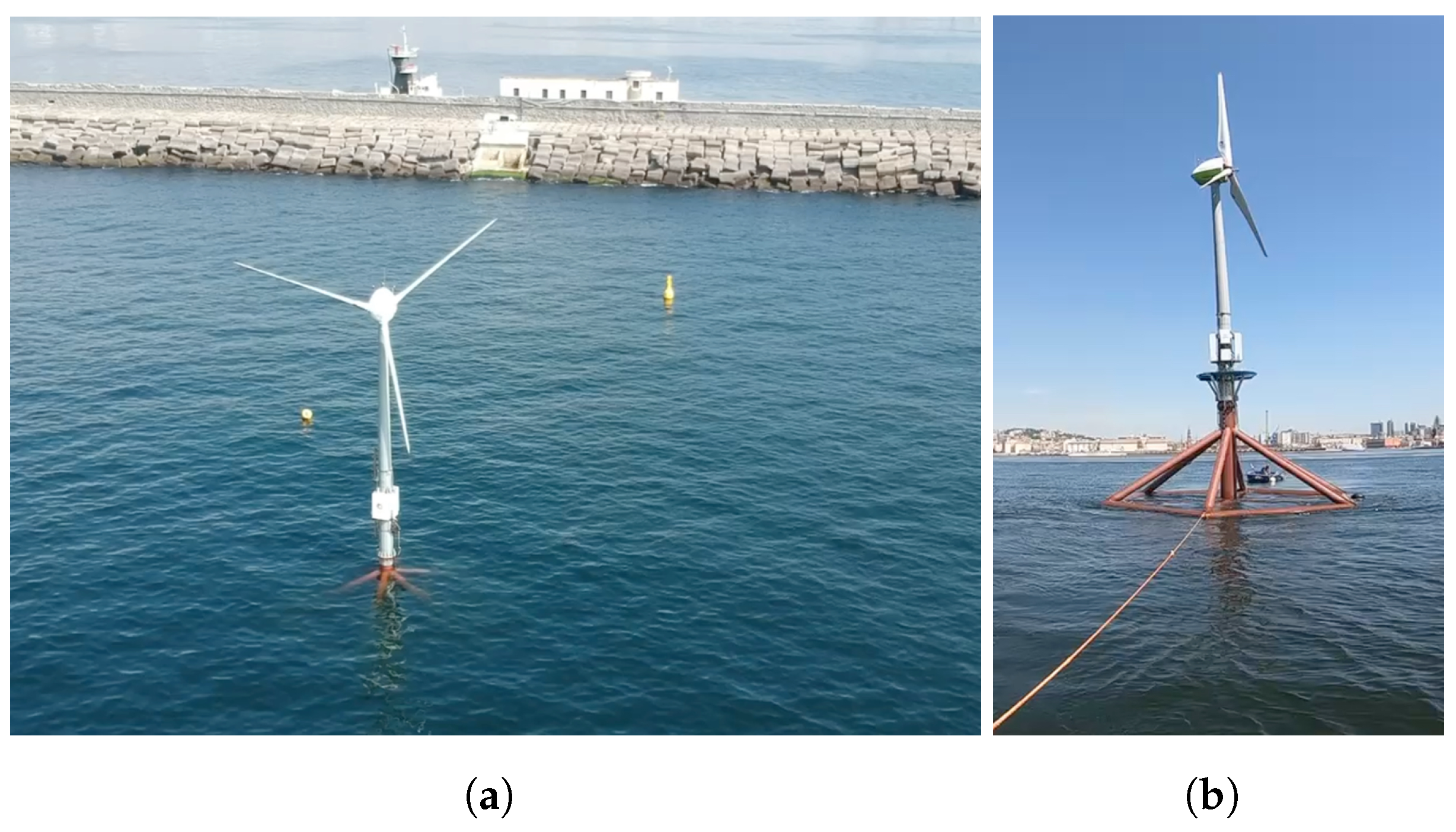
2.1. Wind Turbine Test Case
- The loads applied to one of the three moorings of the platform () and three of the six tendons connecting the counterweight to the floater (, , and ), as measured by a system of underwater load cells LCM5404 with work limit load (WLL) of tons and tons.
- The acceleration along three coordinate axes (, , ), the pitch and roll angles (, ), and the respective angular rates (, ) collected by a Norwegian Subsea MRU 3000 inertial motion unit.
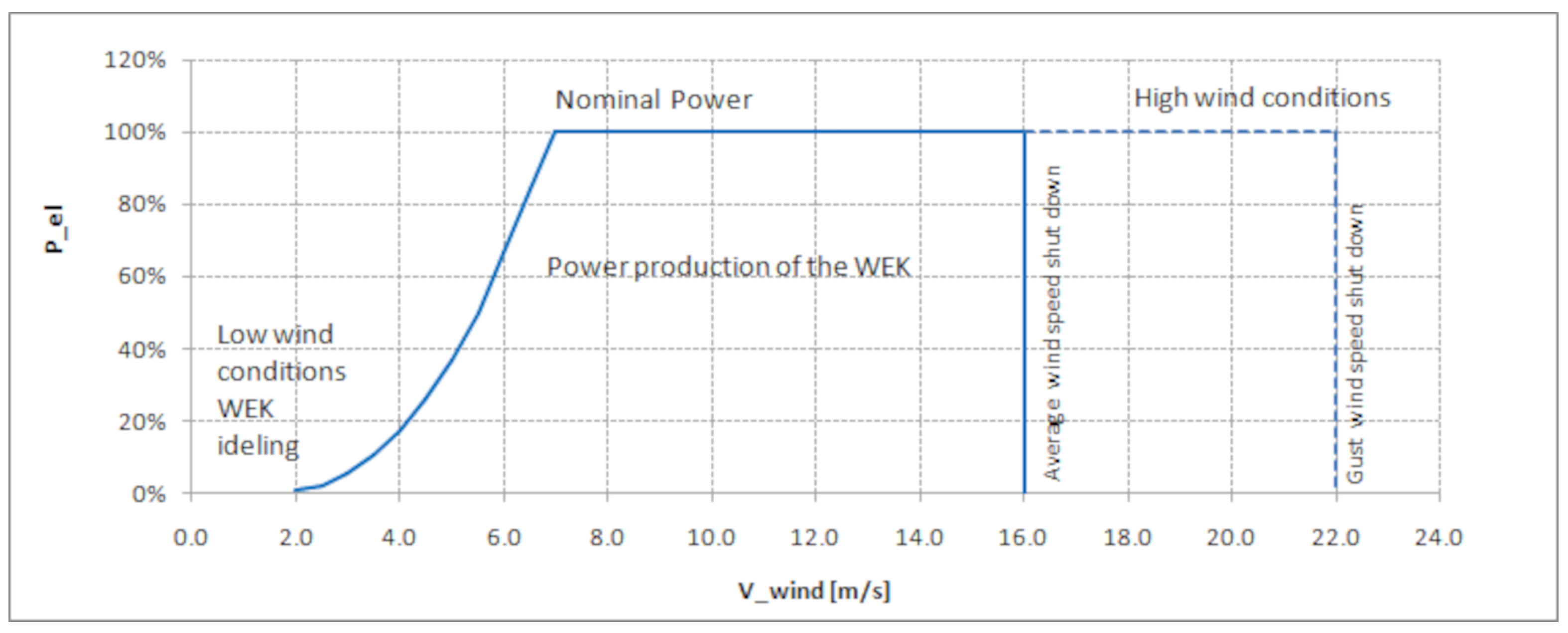
- The power extracted by the wind turbine (P) estimated by a programmable logic controller (PLC) through a direct measure of the electrical quantities at the generator on board the nacelle of the wind turbine, the rotor angular velocity () measured by two sensors in continuous cross-check, and the relative wind speed () through two different anemometers positioned on the nacelle, behind the rotor. All signals were collected by the PLC on the nacelle with a variable but well-known sample frequency of approximately 1 Hz.
- The wave elevation () measured by a pressure transducer integrated into the Acoustic Doppler Current Profiler (ADCP) Teledyne Marine Sentinel V20, located at a distance of approximately 50 m from the FOWT in the southeast direction.
2.2. Dynamic Mode Decomposition
2.3. Dynamic Mode Decomposition with Control
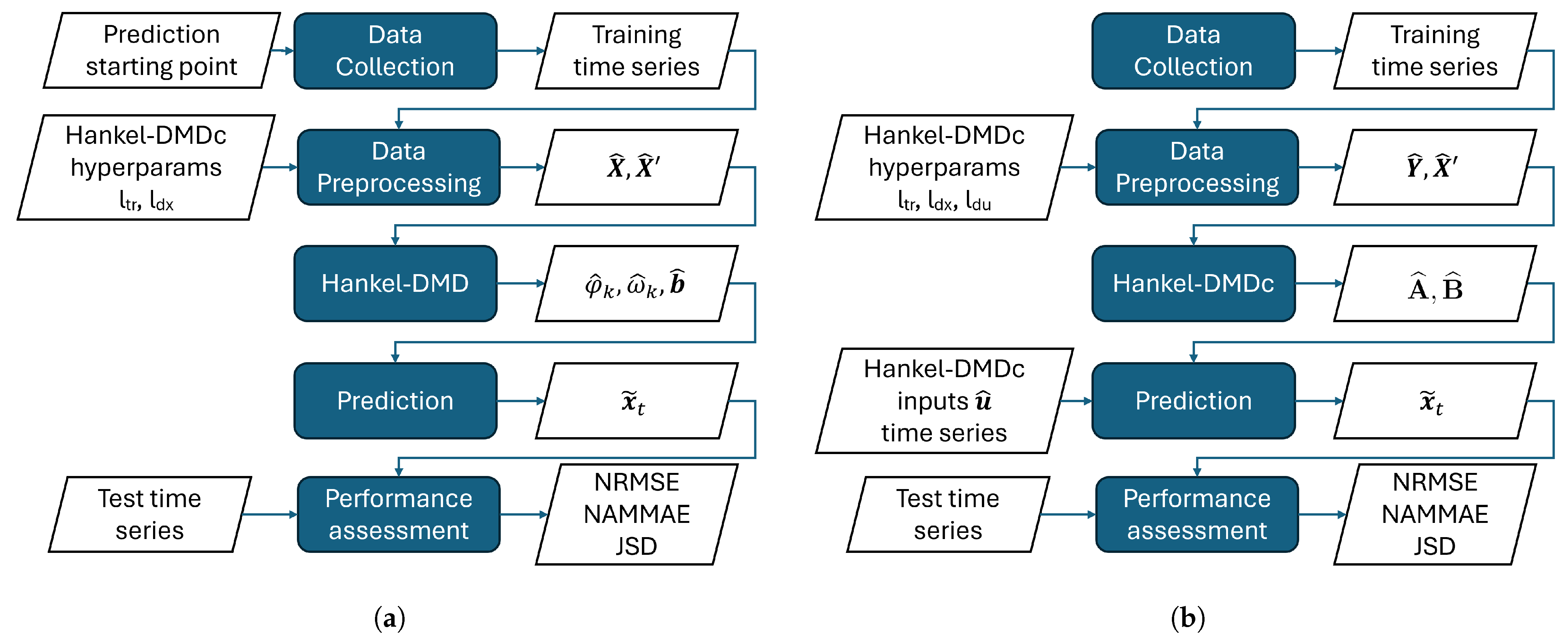
2.4. Hankel Extension to DMD and DMDc
2.5. Bayesian Extension to Hankel-DMD and Hankel-DMDc
3. Performance Metrics
- -
- The NRMSE evidences phase, frequency, and amplitude errors between the reference and the predicted signal, evaluating a pointwise difference between the two. However, it is not possible to discern between the three types of error and to what extent each type contributes to the overall value.
- -
- The NAMMAE indicates if the prediction varies in the same range of the original signal, but it does not give any hint about the phase or frequency similarity of the two.
- -
- The JSD index is ineffective in detecting phase errors between the predicted and the reference signals and is scarcely able to detect infrequent but large amplitude errors. Instead, it highlights whether the compared time histories assume each value in their range of variation a similar number of times. Hence, it is sensitive to errors in the frequency and trend of the predicted signal.
4. Numerical Setup
5. Results
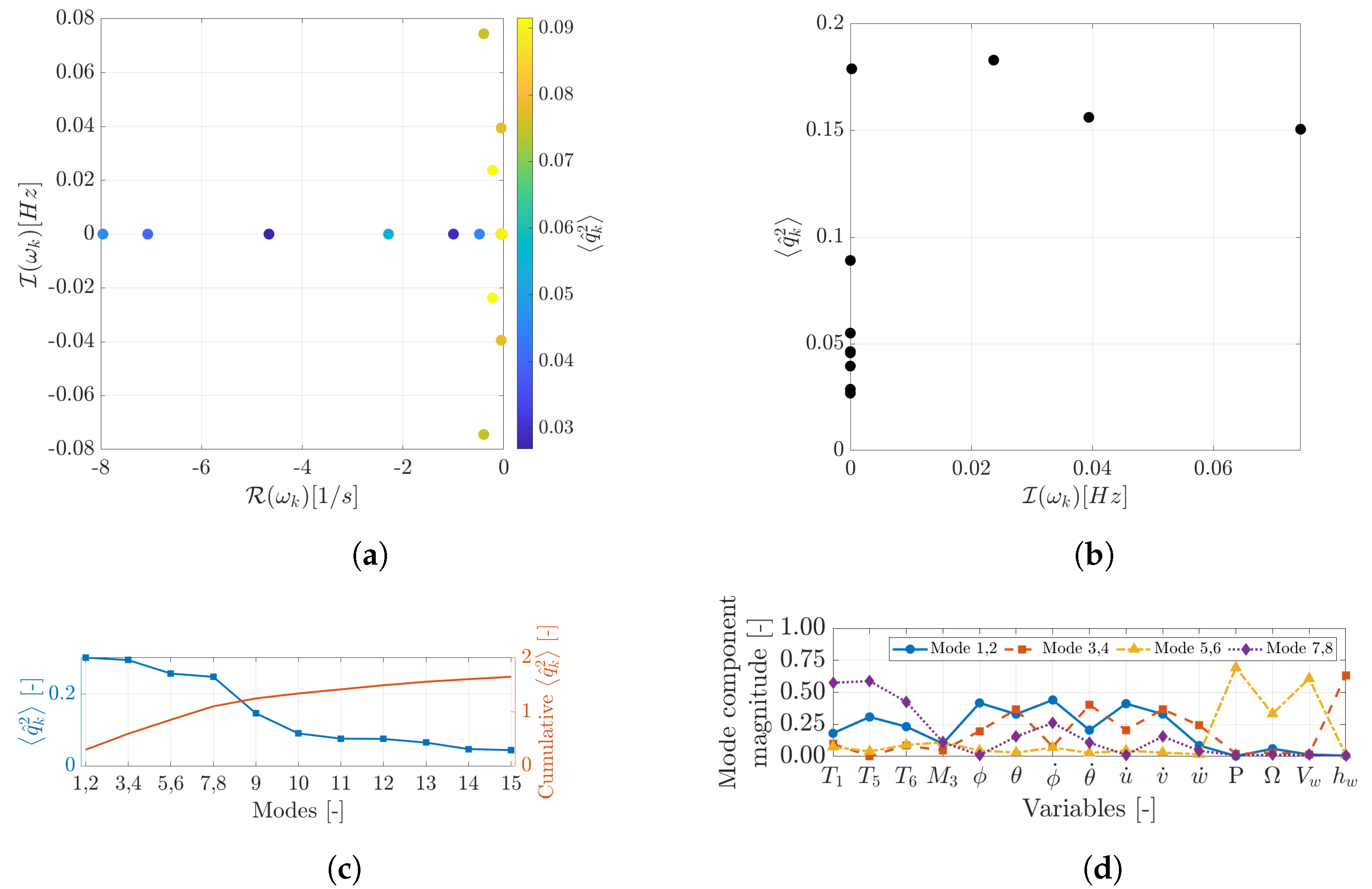
5.1. Modal Analysis
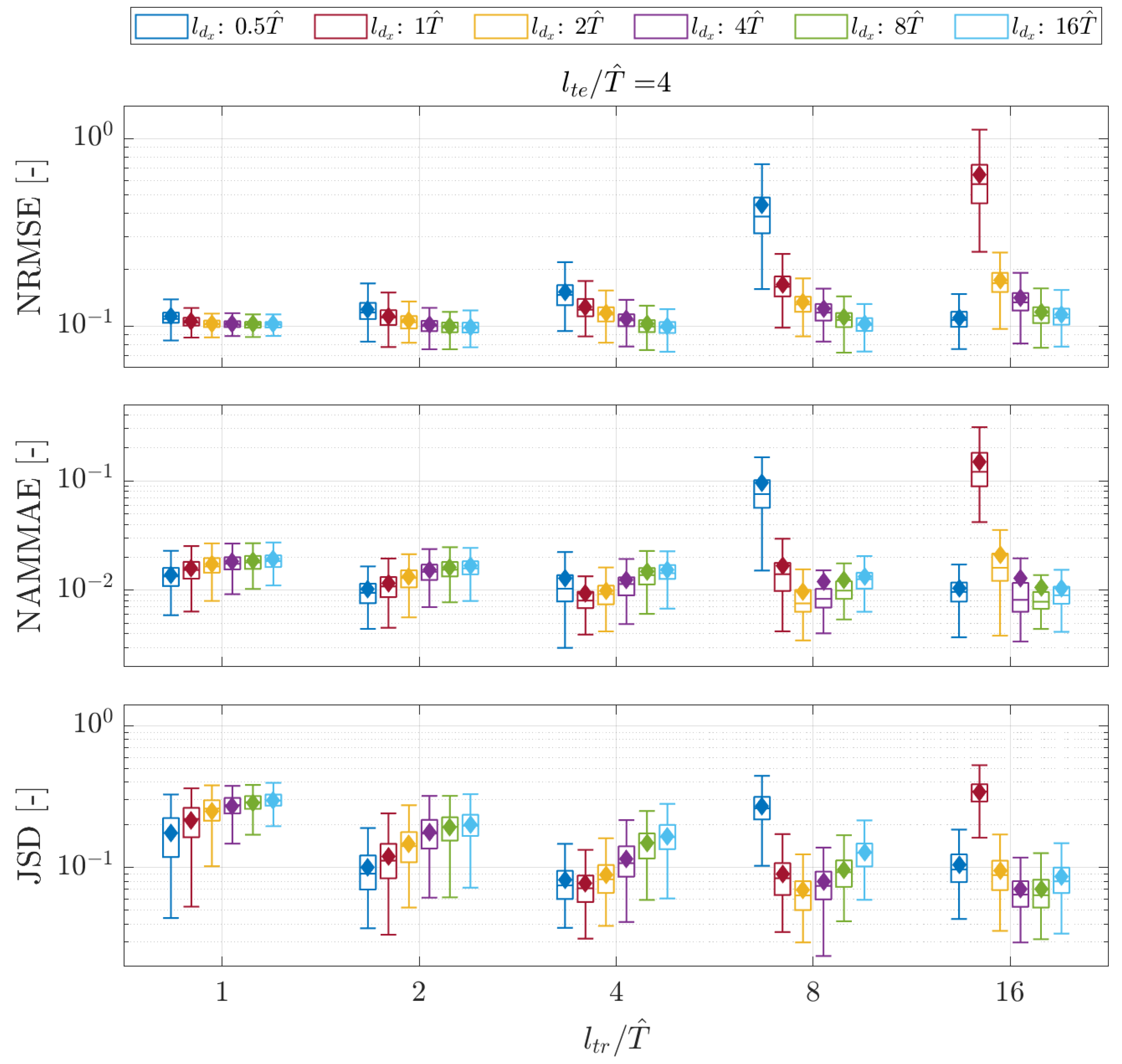
5.2. Nowcasting via Hankel-DMD
- (a)
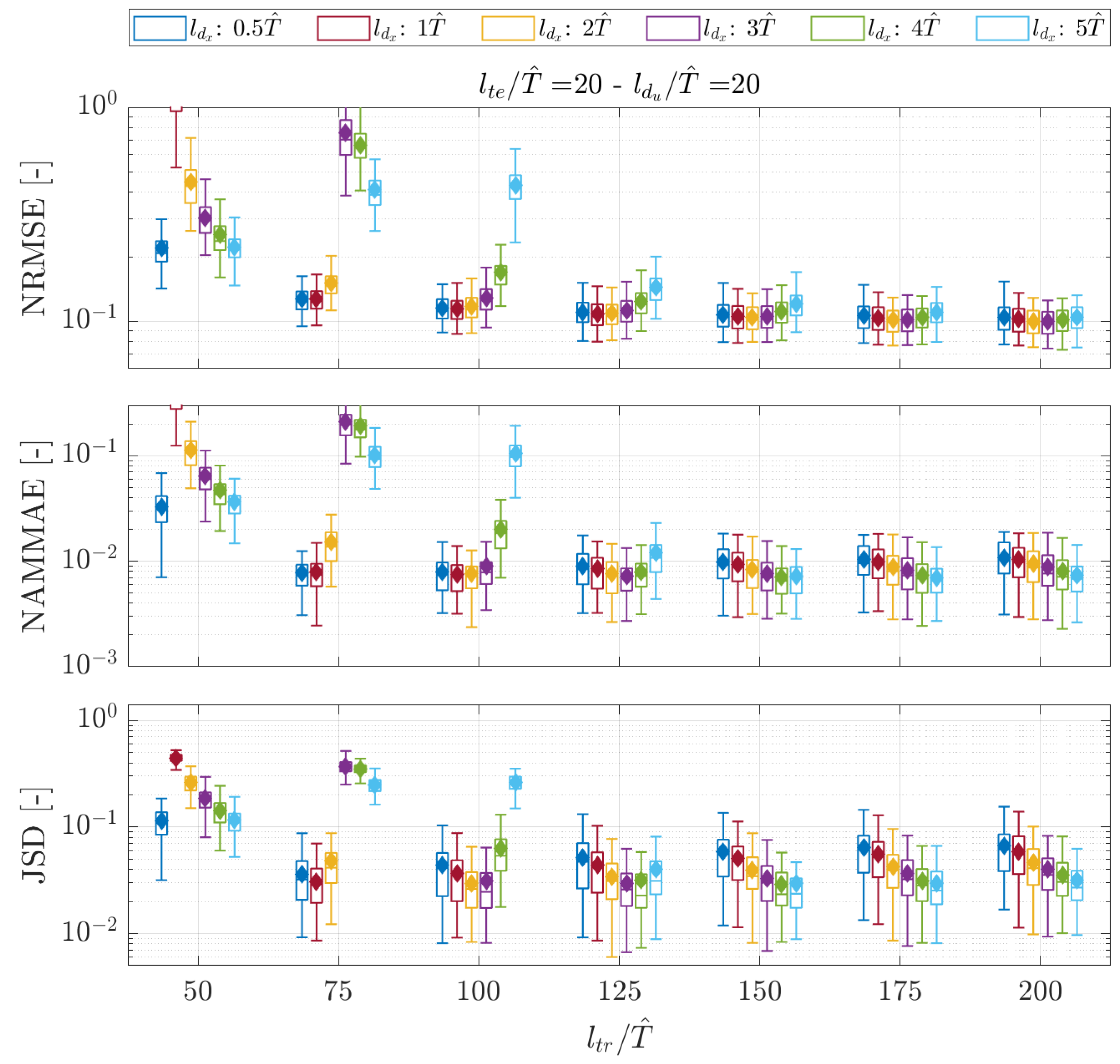
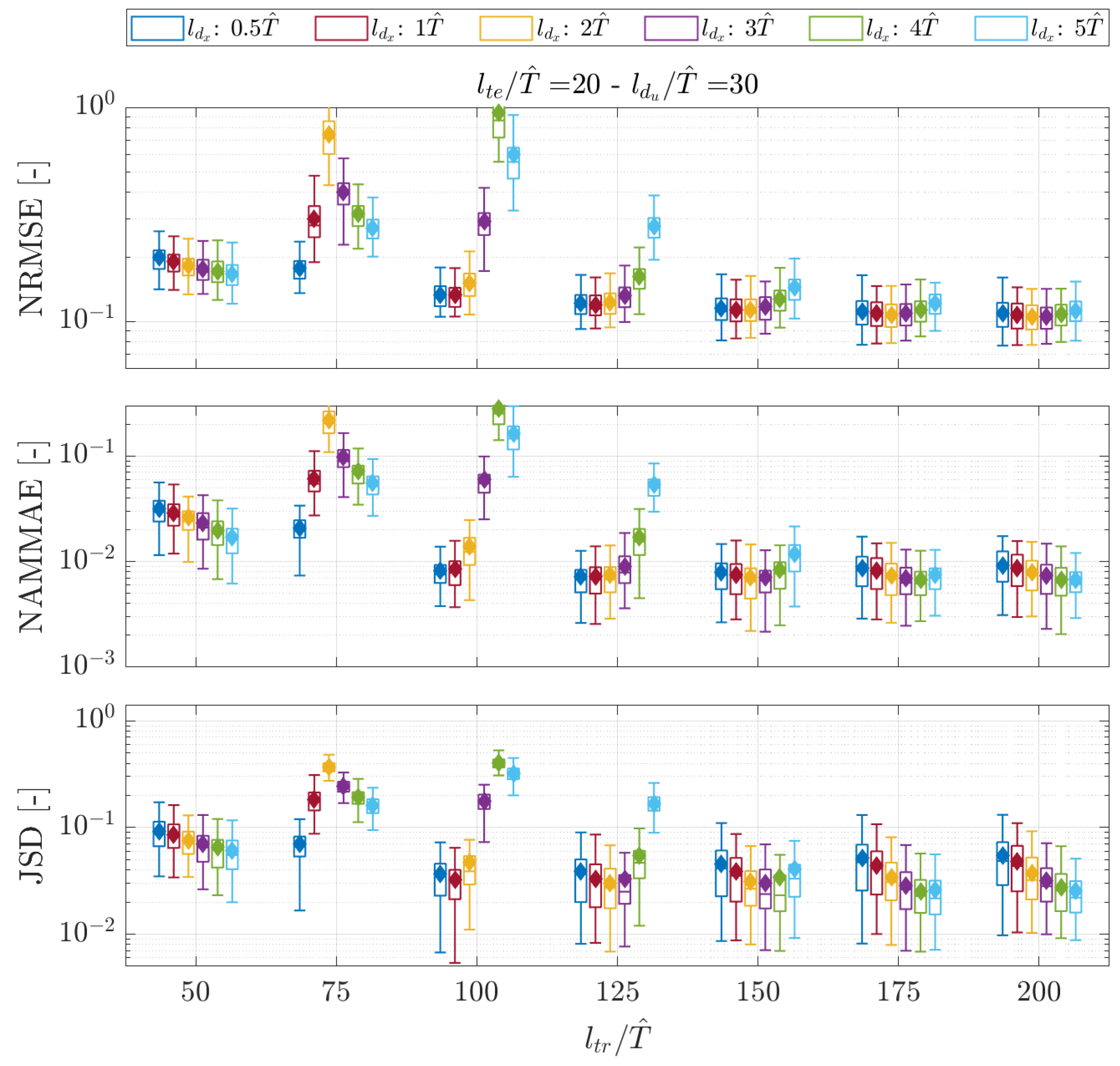
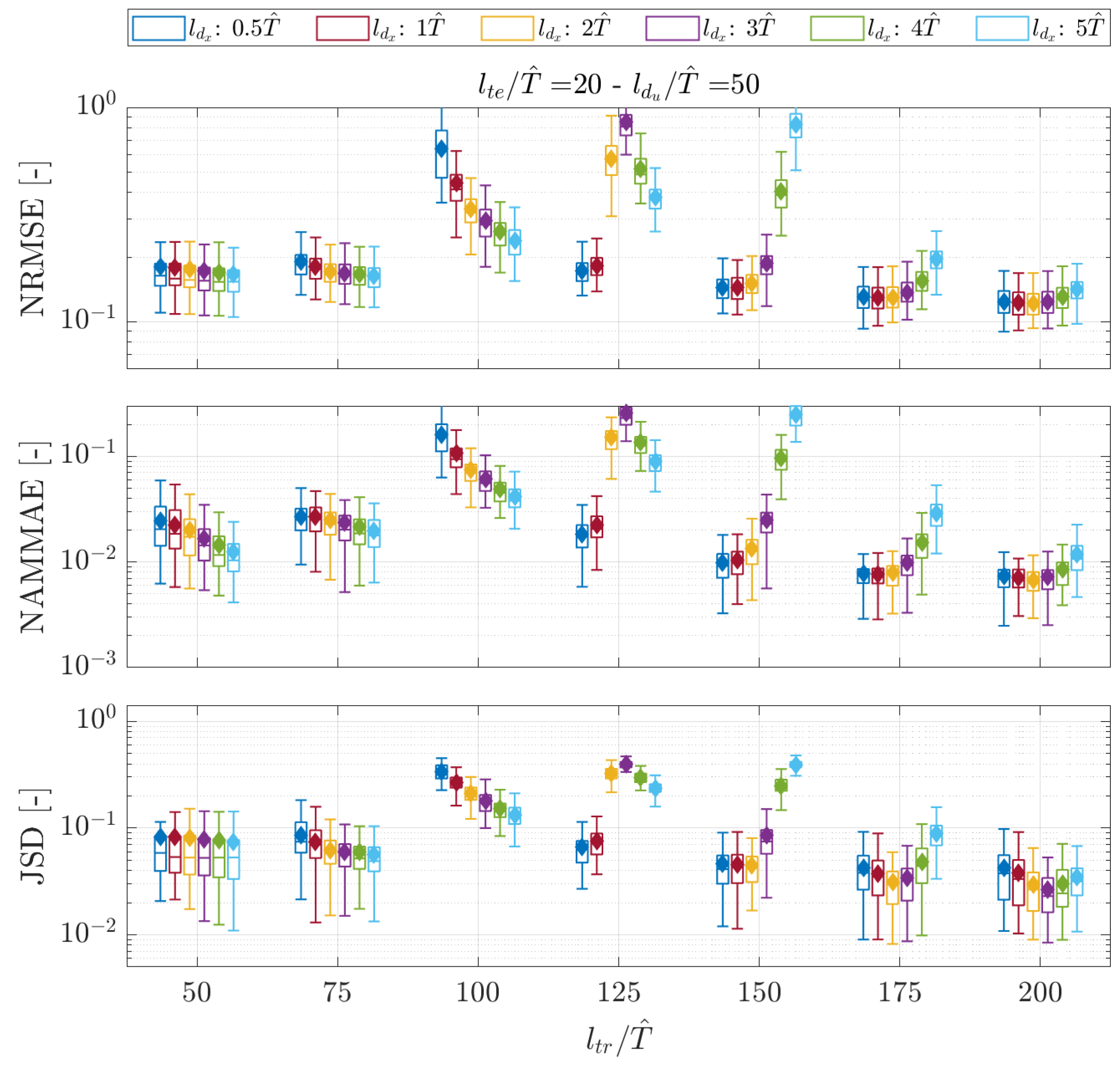
- Long training signals with few delayed copies in the augmented state showed poor prediction capabilities, as confirmed by all the metrics for both the short-term and mid-term time windows. The effect is notable for .
- (b)
- A high number of embedded time-delayed signals with insufficiently long training lengths was prone to producing NRMSEs, progressively reducing the metric’s dispersion around the value of an eighth of the standard deviation of the observed signals. This happens, with the explored values of , particularly for , , and, to a lesser extent, when exceeded 1. At the same time, the NAMMAE and JSD values for the same settings are progressively increasing their values; this indicates that the predicted signals are not able to catch the maximum and minimum values of the reference sequences and that the distribution of the predicted data is not adherent to the true data advancing in time. The combination of those two behaviors is due to the method generating numerous rapidly decaying predictions, whose signals become highly damped after a short observation time.
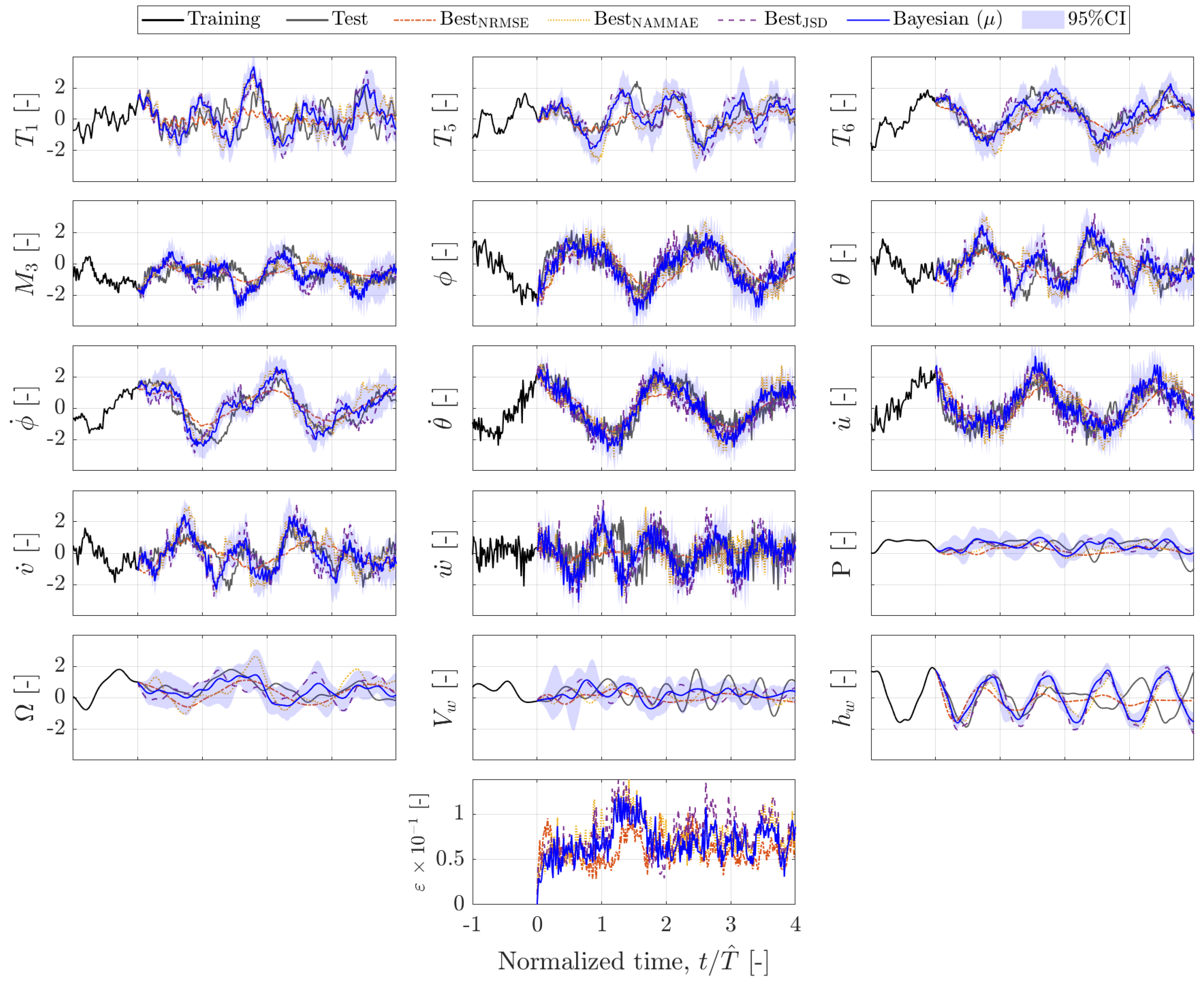
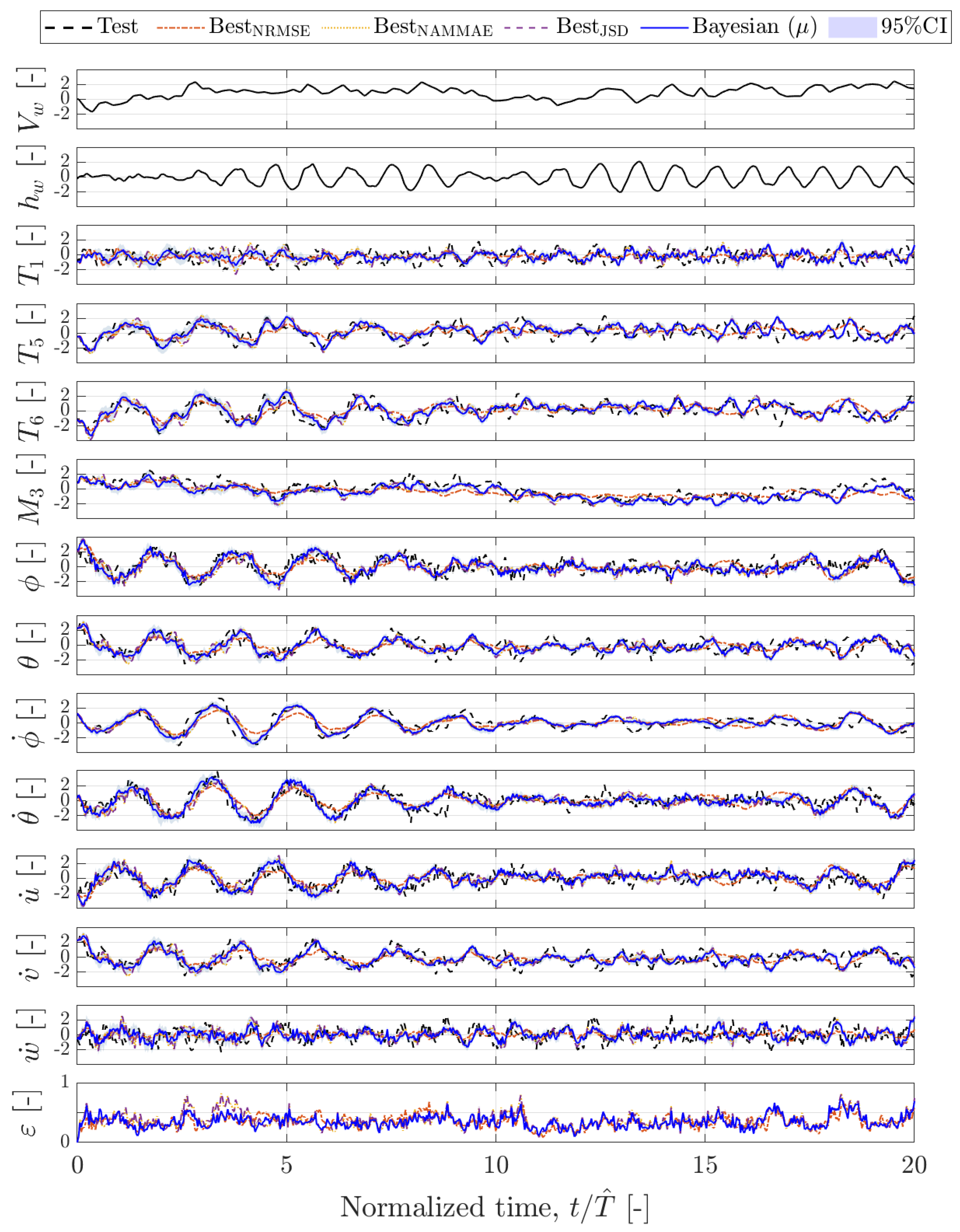
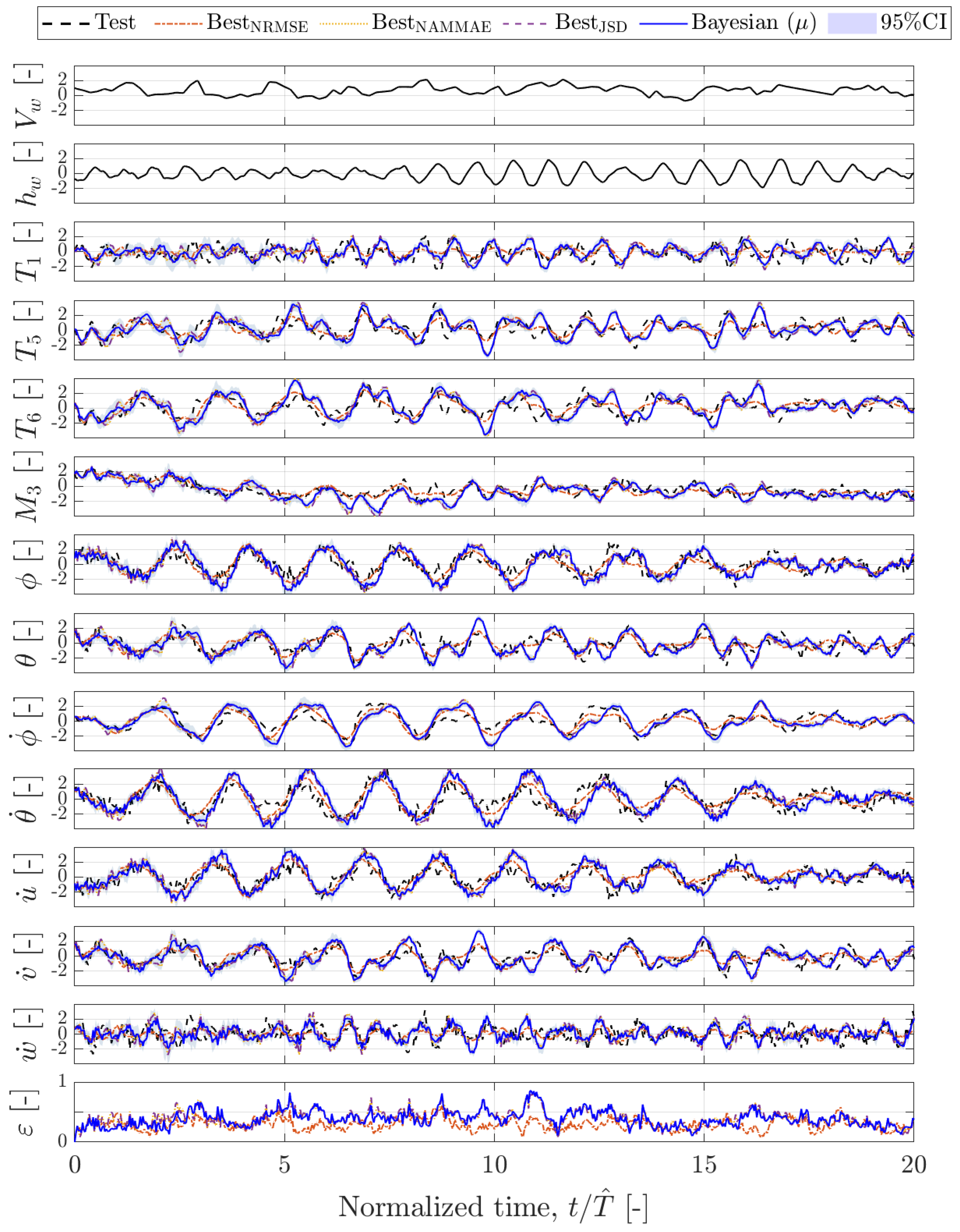
5.3. Nowcasting via Bayesian Hankel-DMD
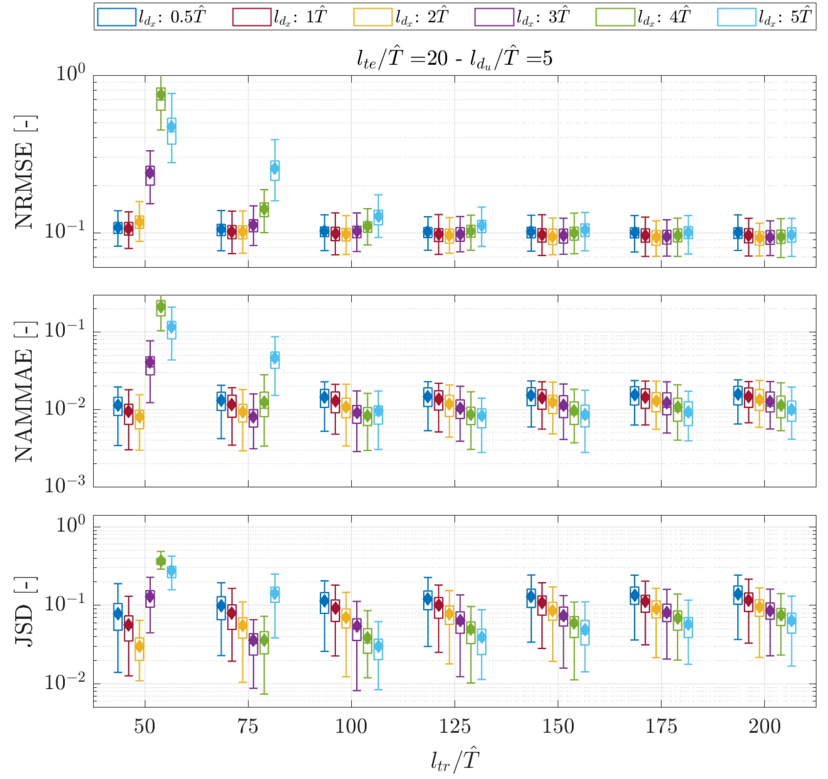
5.4. System Identification via Hankel-DMDc
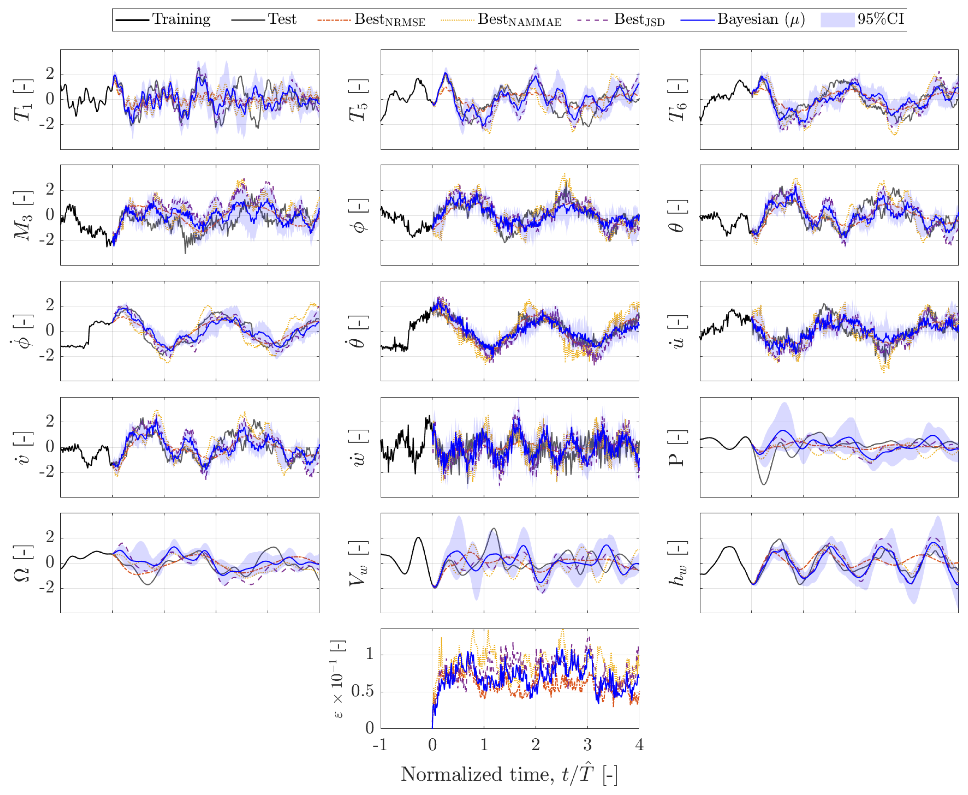
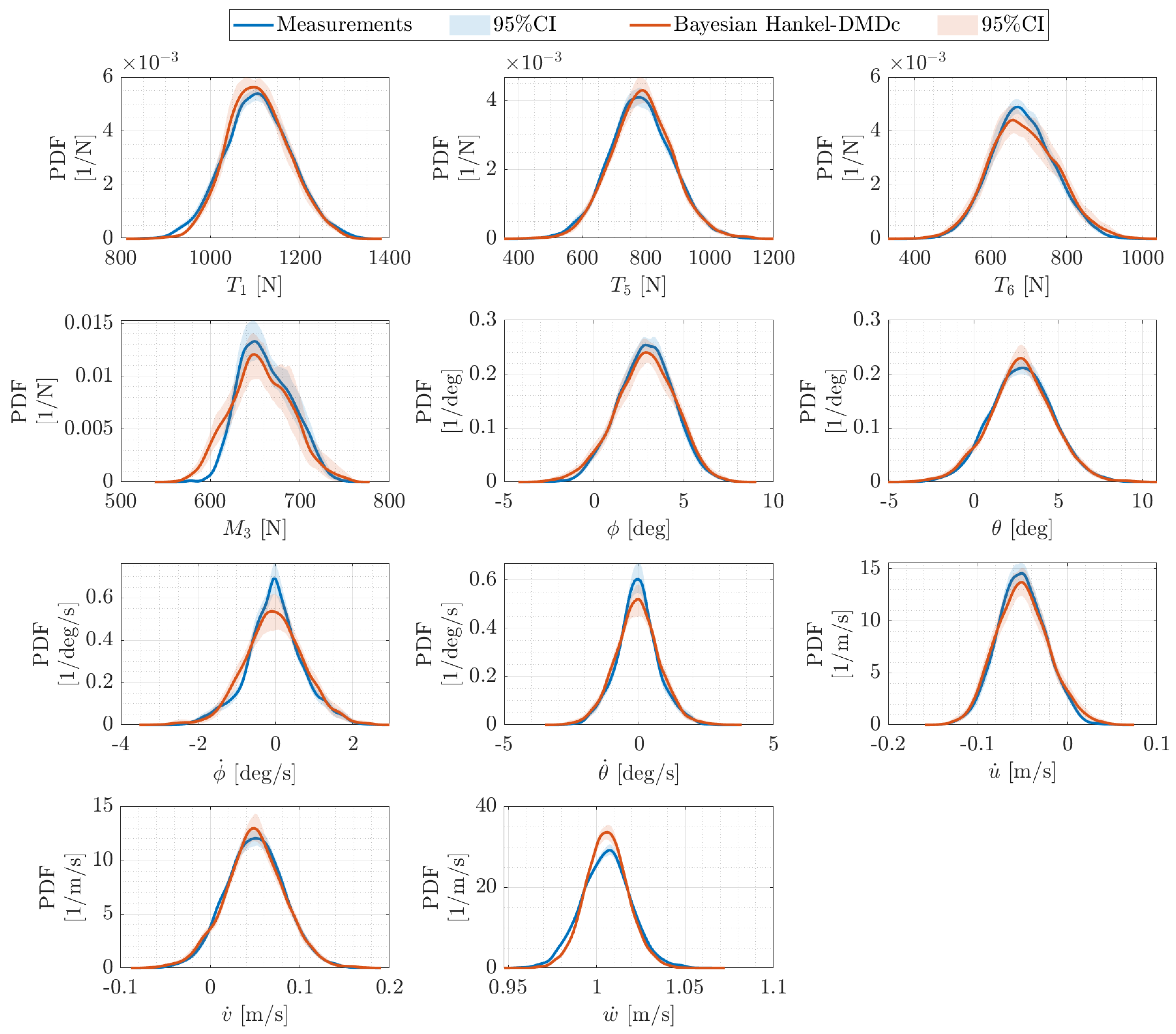
5.5. System Identification via Bayesian Hankel-DMDc
6. Conclusions
Author Contributions
Funding
Data Availability Statement
Conflicts of Interest
List of Symbols and Abbreviations
| Abbreviations | |
| ADCP | acoustic doppler current profiler |
| DMDc | dynamic mode decomposition with control |
| DMD | dynamic mode decomposition |
| EMD | empirical mode decomposition |
| EU | European Union |
| FOWT | floating offshore wind turbine |
| GRNN | gated recurrent neural network |
| JSD | Jensen-Shannon divergence |
| LCOE | levelized cost of energy |
| LSTM | long short-term memory |
| MBB | moving block bootstrap |
| NAMMAE | normalized average minimum/maximum absolute error |
| NRMSE | normalized mean square error |
| probability density function | |
| PLC | programmable logic controller |
| POD | proper orthogonal decomposition |
| ROM | reduced order model |
| SVD | singular value decomposition |
| Greek symbols | |
| time history of the expected value of the components of the vector | |
| time history of the standard deviation of the components of the vector | |
| time step for discretization | |
| floater roll velocity | |
| floater pitch velocity | |
| expected value of | |
| wind turbine rotor angular velocity | |
| k-th eigenvalue of , | |
| floater roll angle | |
| standard deviation of | |
| floater pitch angle | |
| k-th eigenvector of | |
| Symbols | |
| Hermitian transpose operator on | |
| non conjugate transpose operator on | |
| Moore-Penrose pseudoinverse of | |
| j-th time snapshot of , | |
| floater acceleration along x direction | |
| floater acceleration along y direction | |
| floater acceleration along z direction | |
| augmented system state vector | |
| snapshot of the augmented system state vector | |
| floater wave encounter frequency | |
| floater wave encounter period. reference period for non-dimensional time | |
| inner product | |
| discrete time system state matrix | |
| discrete time system input matrix | |
| matrix collecting delayed system state vector snapshots excluding the first | |
| matrix collecting delayed system state vector snapshots excluding the last | |
| augmented system input vector | |
| system input vector | |
| matrix collecting system state vector snapshots excluding the first | |
| matrix collecting system state vector snapshots excluding the last | |
| system state vector | |
| initial condition of the system state vector | |
| matrix collecting delayed system input vector snapshots excluding the last | |
| continuous time system matrix | |
| augmented discrete time system state matrix | |
| augmented discrete time system input matrix | |
| i-th coordinate of the initial condition in the eigenvector basis | |
| wave elevation | |
| maximum delay time in augmented input | |
| maximum delay time in augmented state | |
| test signal time length | |
| training signal time length | |
| number of maximum delay samples in augmented input | |
| number of maximum delay samples in augmented state | |
| number of samples in training signal | |
| P | power extracted by the wind turbine |
| t | time |
| relative wind speed at the wind turbine rotor | |
| load at the i-th mooring of the FOWT platform | |
| load at the i-th tendon of the floater counterweight |
References
- Falkner, R. The Paris Agreement and the new logic of international climate politics. Int. Aff. 2016, 92, 1107–1125. [Google Scholar]
- Nastasi, B.; Markovska, N.; Puksec, T.; Duić, N.; Foley, A. Renewable and sustainable energy challenges to face for the achievement of Sustainable Development Goals. Renew. Sustain. Energy Rev. 2022, 157, 112071. [Google Scholar] [CrossRef]
- International Energy Agency (IEA). Net Zero by 2050; IEA: Paris, France, 2021. [Google Scholar]
- The European Parliament and Council. Directive (EU) 2018/2001 of the European Parliament and of the Council of 11 December 2018 on the Promotion of the Use of Energy from Renewable Sources; The European Parliament and Council: Brussels, Belgium, 2018. [Google Scholar]
- Prakash, G.; Anuta, H.; Wagner, N.; Gallina, G.; Gielen, D.; Gorini, R. Future of Wind-Deployment, Investment, Technology, Grid Integration and Socio-Economic Aspects; International Renewable Energy Agency (IRENA): Masdar City, Abu Dhabi, 2019. [Google Scholar]
- Konstantinidis, E.I.; Botsaris, P.N. Wind turbines: Current status, obstacles, trends and technologies. IOP Conf. Ser. Mater. Sci. Eng. 2016, 161, 012079. [Google Scholar] [CrossRef]
- Pustina, L.; Lugni, C.; Bernardini, G.; Serafini, J.; Gennaretti, M. Control of power generated by a floating offshore wind turbine perturbed by sea waves. Renew. Sustain. Energy Rev. 2020, 132, 109984. [Google Scholar] [CrossRef]
- Pustina, L.; Serafini, J.; Pasquali, C.; Solero, L.; Lidozzi, A.; Gennaretti, M. A novel resonant controller for sea-induced rotor blade vibratory loads reduction on floating offshore wind turbines. Renew. Sustain. Energy Rev. 2023, 173, 113073. [Google Scholar] [CrossRef]
- López-Queija, J.; Robles, E.; Jugo, J.; Alonso-Quesada, S. Review of control technologies for floating offshore wind turbines. Renew. Sustain. Energy Rev. 2022, 167, 112787. [Google Scholar] [CrossRef]
- Global Wind Energy Council (GWEC). Global Offshore Wind Report 2020; GWEC: Brussels, Belgium, 2020; Volume 19, pp. 10–12. [Google Scholar]
- McMorland, J.; Collu, M.; McMillan, D.; Carroll, J. Operation and maintenance for floating wind turbines: A review. Renew. Sustain. Energy Rev. 2022, 163, 112499. [Google Scholar] [CrossRef]
- Florian, M.; Sørensen, J.D. Wind Turbine Blade Life-Time Assessment Model for Preventive Planning of Operation and Maintenance. J. Mar. Sci. Eng. 2015, 3, 1027–1040. [Google Scholar] [CrossRef]
- de Azevedo, H.D.M.; Araújo, A.M.; Bouchonneau, N. A review of wind turbine bearing condition monitoring: State of the art and challenges. Renew. Sustain. Energy Rev. 2016, 56, 368–379. [Google Scholar] [CrossRef]
- Jonkman, J. Dynamics Modeling and Loads Analysis of an Offshore Floating Wind Turbine; University of Colorado at Boulder: Boulder, CO, USA, 2007. [Google Scholar] [CrossRef]
- Si, Y.; Karimi, H.R.; Gao, H. Modelling and optimization of a passive structural control design for a spar-type floating wind turbine. Eng. Struct. 2014, 69, 168–182. [Google Scholar] [CrossRef]
- Li, X.; Gao, H. Load Mitigation for a Floating Wind Turbine via Generalized H∞ Structural Control. IEEE Trans. Ind. Electron. 2016, 63, 332–342. [Google Scholar] [CrossRef]
- Dong, H.; Edrah, M.; Zhao, X.; Collu, M.; Xu, X.; K A, A.; Lin, Z. Model-Free Semi-Active Structural Control of Floating Wind Turbines. In Proceedings of the 2020 Chinese Automation Congress (CAC), Shanghai, China, 6–8 November 2020; pp. 4216–4220. [Google Scholar] [CrossRef]
- Tetteh, E.Y.; Fletcher, K.; Qin, C.; Loth, E.; Damiani, R. Active Ballasting Actuation for the SpiderFLOAT Offshore Wind Turbine Platform. In Proceedings of the AIAA SCITECH 2022 Forum, San Diego, CA, USA, 3–7 January 2022. [Google Scholar] [CrossRef]
- Galván, J.; Sánchez-Lara, M.J.; Mendikoa, I.; Pérez-Morán, G.; Nava, V.; Rodríguez-Arias, R. NAUTILUS-DTU10 MW Floating Offshore Wind Turbine at Gulf of Maine: Public numerical models of an actively ballasted semisubmersible. J. Phys. Conf. Ser. 2018, 1102, 012015. [Google Scholar] [CrossRef]
- Grant, E.; Johnson, K.; Damiani, R.; Phadnis, M.; Pao, L. Buoyancy can ballast control for increased power generation of a floating offshore wind turbine with a light-weight semi-submersible platform. Appl. Energy 2023, 330, 120287. [Google Scholar] [CrossRef]
- Palraj, M.; Rajamanickam, P. Motion control studies of a barge mounted offshore dynamic wind turbine using gyrostabilizer. Ocean. Eng. 2021, 237, 109578. [Google Scholar] [CrossRef]
- Salic, T.; Charpentier, J.F.; Benbouzid, M.; Le Boulluec, M. Control Strategies for Floating Offshore Wind Turbine: Challenges and Trends. Electronics 2019, 8, 1185. [Google Scholar] [CrossRef]
- Tiwari, R.; Babu, N.R. Recent developments of control strategies for wind energy conversion system. Renew. Sustain. Energy Rev. 2016, 66, 268–285. [Google Scholar] [CrossRef]
- Awada, A.; Younes, R.; Ilinca, A. Review of Vibration Control Methods for Wind Turbines. Energies 2021, 14, 3058. [Google Scholar] [CrossRef]
- Larsen, T.J.; Hanson, T.D. A method to avoid negative damped low frequent tower vibrations for a floating, pitch controlled wind turbine. J. Phys. Conf. Ser. 2007, 75, 012073. [Google Scholar] [CrossRef]
- Jonkman, J. Influence of Control on the Pitch Damping of a Floating Wind Turbine. In Proceedings of the 46th AIAA Aerospace Sciences Meeting and Exhibit, Reno, NV, USA, 7–10 January 2008. [Google Scholar] [CrossRef]
- Yu, W.; Lemmer, F.; Schlipf, D.; Cheng, P.W.; Visser, B.; Links, H.; Gupta, N.; Dankemann, S.; Counago, B.; Serna, J. Evaluation of control methods for floating offshore wind turbines. J. Phys. Conf. Ser. 2018, 1104, 012033. [Google Scholar] [CrossRef]
- Bakka, T.; Karimi, H. Robust H∞ Dynamic Output Feedback Control Synthesis with Pole Placement Constraints for Offshore Wind Turbine Systems. Math. Probl. Eng. 2012, 2012, 616507. [Google Scholar] [CrossRef]
- Betti, G.; Farina, M.; Marzorati, A.; Scattolini, R.; Guagliardi, G.A. Modeling and control of a floating wind turbine with spar buoy platform. In Proceedings of the 2012 IEEE International Energy Conference and Exhibition (ENERGYCON), Florence, Italy, 9–12 September 2012; pp. 189–194. [Google Scholar] [CrossRef]
- Lemmer (né Sandner), F.; Yu, W.; Schlipf, D.; Cheng, P.W. Robust gain scheduling baseline controller for floating offshore wind turbines. Wind. Energy 2020, 23, 17–30. [Google Scholar] [CrossRef]
- Sarkar, S.; Fitzgerald, B.; Basu, B. Individual Blade Pitch Control of Floating Offshore Wind Turbines for Load Mitigation and Power Regulation. IEEE Trans. Control Syst. Technol. 2021, 29, 305–315. [Google Scholar] [CrossRef]
- Harris, M.; Hand, M.; Wright, A. Lidar for Turbine Control: March 1, 2005-November 30, 2005; Technical Report; NREL—National Wind Technology Center: Boulder, CO, USA, 2006. [Google Scholar] [CrossRef]
- Laks, J.; Pao, L.; Wright, A.; Kelley, N.; Jonkman, B. Blade Pitch Control with Preview Wind Measurements. In Proceedings of the 48th AIAA Aerospace Sciences Meeting Including the New Horizons Forum and Aerospace Exposition, Orlando, FL, USA, 4–7 January 2010; American Institute of Aeronautics and Astronautics: Reston, VA, USA, 2010. Chapter 2010-251. pp. 1–24. [Google Scholar] [CrossRef]
- Dunne, F.; Pao, L.; Wright, A.; Jonkman, B.; Kelley, N. Combining Standard Feedback Controllers with Feedforward Blade Pitch Control for Load Mitigation in Wind Turbines. In Proceedings of the 48th AIAA Aerospace Sciences Meeting Including the New Horizons Forum and Aerospace Exposition, Orlando, FL, USA, 4–7 January 2010; American Institute of Aeronautics and Astronautics: Reston, VA, USA, 2010. Chapter AIAA 2010-250. pp. 1–18. [Google Scholar] [CrossRef]
- Dunne, F.; Pao, L.; Wright, A.; Jonkman, B.; Kelley, N.; Simley, E. Adding Feedforward Blade Pitch Control for Load Mitigation in Wind Turbines: Non-Causal Series Expansion, Preview Control, and Optimized FIR Filter Methods. In Proceedings of the 49th AIAA Aerospace Sciences Meeting including the New Horizons Forum and Aerospace Exposition, Orlando, FL, USA, 4–7 January 2011; American Institute of Aeronautics and Astronautics: Reston, VA, USA, 2011. Chapter 2011-819. pp. 1–17. [Google Scholar] [CrossRef]
- Dunne, F.; Schlipf, D.; Pao, L.; Wright, A.; Jonkman, B.; Kelley, N.; Simley, E. Comparison of Two Independent Lidar-Based Pitch Control Designs. In Proceedings of the 50th AIAA Aerospace Sciences Meeting including the New Horizons Forum and Aerospace Exposition, Nashville, TN, USA, 9–12 January 2012; American Institute of Aeronautics and Astronautics: Reston, VA, USA, 2012. Chapter 2012-1151. pp. 1–19. [Google Scholar] [CrossRef]
- Raach, S.; Schlipf, D.; Sandner, F.; Matha, D.; Cheng, P.W. Nonlinear model predictive control of floating wind turbines with individual pitch control. In Proceedings of the 2014 American Control Conference, Portland, OR, USA, 4–6 June 2014; pp. 4434–4439. [Google Scholar] [CrossRef]
- Schlipf, D.; Simley, E.; Lemmer, F.; Pao, L.; Cheng, P.W. Collective Pitch Feedforward Control of Floating Wind Turbines Using Lidar. J. Ocean. Wind. Energy 2015, 2. [Google Scholar] [CrossRef]
- Ma, Y.; Sclavounos, P.D.; Cross-Whiter, J.; Arora, D. Wave forecast and its application to the optimal control of offshore floating wind turbine for load mitigation. Renew. Energy 2018, 128, 163–176. [Google Scholar] [CrossRef]
- Simley, E.; Bortolotti, P.; Scholbrock, A.; Schlipf, D.; Dykes, K. IEA Wind Task 32 and Task 37: Optimizing Wind Turbines with Lidar-Assisted Control Using Systems Engineering. J. Phys. Conf. Ser. 2020, 1618, 042029. [Google Scholar] [CrossRef]
- Fontanella, A.; Al, M.; van Wingerden, J.W.; Belloli, M. Model-based design of a wave-feedforward control strategy in floating wind turbines. Wind. Energy Sci. 2021, 6, 885–901. [Google Scholar] [CrossRef]
- Al, M.; Fontanella, A.; van der Hoek, D.; Liu, Y.; Belloli, M.; van Wingerden, J.W. Feedforward control for wave disturbance rejection on floating offshore wind turbines. J. Phys. Conf. Ser. 2020, 1618, 022048. [Google Scholar] [CrossRef]
- Otter, A.; Murphy, J.; Pakrashi, V.; Robertson, A.; Desmond, C. A review of modelling techniques for floating offshore wind turbines. Wind. Energy 2022, 25, 831–857. [Google Scholar] [CrossRef]
- Høeg, C.E.; Zhang, Z. A semi-analytical hydrodynamic model for floating offshore wind turbines (FOWT) with application to a FOWT heave plate tuned mass damper. Ocean. Eng. 2023, 287, 115756. [Google Scholar] [CrossRef]
- Wang, K.; Gaidai, O.; Wang, F.; Xu, X.; Zhang, T.; Deng, H. Artificial Neural Network-Based Prediction of the Extreme Response of Floating Offshore Wind Turbines under Operating Conditions. J. Mar. Sci. Eng. 2023, 11, 1807. [Google Scholar] [CrossRef]
- Zhang, Y.; Yang, X.; Liu, S. Data-driven predictive control for floating offshore wind turbines based on deep learning and multi-objective optimization. Ocean. Eng. 2022, 266, 112820. [Google Scholar] [CrossRef]
- Barooni, M.; Velioglu Sogut, D. Forecasting Pitch Response of Floating Offshore Wind Turbines with a Deep Learning Model. Clean Technol. 2024, 6, 418–431. [Google Scholar] [CrossRef]
- Gräfe, M.; Pettas, V.; Cheng, P.W. Data-driven forecasting of FOWT dynamics and load time series using lidar inflow measurements. J. Phys. Conf. Ser. 2024, 2767, 032025. [Google Scholar] [CrossRef]
- Deng, S.; Ning, D.; Mayon, R. The motion forecasting study of floating offshore wind turbine using self-attention long short-term memory method. Ocean. Eng. 2024, 310, 118709. [Google Scholar] [CrossRef]
- Ye, Y.; Wang, L.; Wang, Y.; Qin, L. An EMD-LSTM-SVR model for the short-term roll and sway predictions of semi-submersible. Ocean. Eng. 2022, 256, 111460. [Google Scholar] [CrossRef]
- Song, B.; Zhou, Q.; Chang, R. Short-term motion prediction of FOWT based on time-frequency feature fusion LSTM combined with signal decomposition methods. Ocean. Eng. 2025, 317, 120046. [Google Scholar] [CrossRef]
- Mainini, L.; Diez, M. Digital Twins and their Mathematical Souls. In Proceedings of the STO-MP-AVT 369 Research Symposium on Digital Twin Technology Development and Application for Tri-Service Platforms and Systems, NATO Science and Technology Organization, Båstad, Sweden, 10–12 October 2023. [Google Scholar]
- Schmid, P.J. Dynamic mode decomposition of numerical and experimental data. J. Fluid Mech. 2010, 656, 5–28. [Google Scholar] [CrossRef]
- Kutz, J.; Brunton, S.; Brunton, B.; Proctor, J. Dynamic Mode Decomposition: Data-Driven Modeling of Complex Systems; SIAM—Society for Industrial and Applied Mathematics: Philadelphia, PA, USA, 2016. [Google Scholar]
- Mezić, I. Koopman Operator, Geometry, and Learning of Dynamical Systems. Not. Am. Math. Soc. 2021, 68, 1087–1105. [Google Scholar]
- Arbabi, H.; Mezić, I. Ergodic Theory, Dynamic Mode Decomposition, and Computation of Spectral Properties of the Koopman Operator. SIAM J. Appl. Dyn. Syst. 2017, 16, 2096–2126. [Google Scholar] [CrossRef]
- Brunton, S.L.; Brunton, B.W.; Proctor, J.L.; Kaiser, E.; Kutz, J.N. Chaos as an intermittently forced linear system. Nat. Commun. 2017, 8, 19. [Google Scholar] [CrossRef]
- Kamb, M.; Kaiser, E.; Brunton, S.L.; Kutz, J.N. Time-Delay Observables for Koopman: Theory and Applications. SIAM J. Appl. Dyn. Syst. 2020, 19, 886–917. [Google Scholar] [CrossRef]
- Serani, A.; Dragone, P.; Stern, F.; Diez, M. On the use of dynamic mode decomposition for time-series forecasting of ships operating in waves. Ocean. Eng. 2023, 267, 113235. [Google Scholar] [CrossRef]
- Proctor, J.L.; Brunton, S.L.; Kutz, J.N. Dynamic mode decomposition with control. SIAM J. Appl. Dyn. Syst. 2016, 15, 142–161. [Google Scholar]
- Proctor, J.L.; Brunton, S.L.; Kutz, J.N. Generalizing Koopman Theory to Allow for Inputs and Control. SIAM J. Appl. Dyn. Syst. 2018, 17, 909–930. [Google Scholar]
- Brunton, S.L.; Budišić, M.; Kaiser, E.; Kutz, J.N. Modern Koopman Theory for Dynamical Systems. SIAM Rev. 2022, 64, 229–340. [Google Scholar] [CrossRef]
- Zawacki, C.C.; Abed, E.H. Dynamic Mode Decomposition for Control Systems with Input Delays. IFAC-PapersOnLine 2023, 56, 97–102. [Google Scholar] [CrossRef]
- Dylewsky, D.; Barajas-Solano, D.; Ma, T.; Tartakovsky, A.M.; Kutz, J.N. Stochastically Forced Ensemble Dynamic Mode Decomposition for Forecasting and Analysis of Near-Periodic Systems. IEEE Access 2022, 10, 33440–33448. [Google Scholar] [CrossRef]
- Mohan, N.; Soman, K.; Kumar, S.S. A data-driven strategy for short-term electric load forecasting using dynamic mode decomposition model. Appl. Energy 2018, 232, 229–244. [Google Scholar] [CrossRef]
- Al-Jiboory, A.K. Adaptive quadrotor control using online dynamic mode decomposition. Eur. J. Control 2024, 80, 101117. [Google Scholar] [CrossRef]
- Dawson, S.T.; Schiavone, N.K.; Rowley, C.W.; Williams, D.R. A Data-Driven Modeling Framework for Predicting Forces and Pressures on a Rapidly Pitching Airfoil. In Proceedings of the 45th AIAA Fluid Dynamics Conference, Dallas, TX, USA, 22–26 June 2015; American Institute of Aeronautics and Astronautics: Reston, VA, USA, 2015. Chapter AIAA 2015-2767. pp. 1–14. [Google Scholar] [CrossRef]
- Rowley, C.W.; Mezić, I.; Bagheri, S.; Schlatter, P.; Hennigson, D.S. Spectral analysis of nonlinear flows. J. Fluid Mech. 2009, 641, 115–127. [Google Scholar] [CrossRef]
- Tang, Z.; Jiang, N. Dynamic mode decomposition of hairpin vortices generated by a hemisphere protuberance. Sci. China Phys. Mech. Astron. 2012, 55, 118–124. [Google Scholar] [CrossRef]
- Semeraro, O.; Bellani, G.; Lundell, F. Analysis of time-resolved PIV measurements of a confined turbulent jet using POD and Koopman modes. Exp. Fluids 2012, 53, 1203–1220. [Google Scholar] [CrossRef]
- Song, G.; Alizard, F.; Robinet, J.C.; Gloerfelt, X. Global and Koopman modes analysis of sound generation in mixing layers. Phys. Fluids 2013, 25, 124101. [Google Scholar] [CrossRef]
- Proctor, J.L.; Eckhoff, P.A. Discovering dynamic patterns from infectious disease data using dynamic mode decomposition. Int. Health 2015, 7, 139–145. [Google Scholar] [CrossRef]
- Brunton, B.W.; Johnson, L.A.; Ojemann, J.G.; Kutz, J.N. Extracting spatial—Temporal coherent patterns in large-scale neural recordings using dynamic mode decomposition. J. Neurosci. Methods 2016, 258, 1–15. [Google Scholar] [CrossRef]
- Mann, J.; Kutz, J.N. Dynamic mode decomposition for financial trading strategies. Quant. Financ. 2016, 16, 1643–1655. [Google Scholar] [CrossRef]
- Diez, M.; Serani, A.; Campana, E.F.; Stern, F. Time-series forecasting of ships maneuvering in waves via dynamic mode decomposition. J. Ocean. Eng. Mar. Energy 2022, 8, 471–478. [Google Scholar] [CrossRef]
- Diez, M.; Gaggero, M.; Serani, A. Data-driven forecasting of ship motions in waves using machine learning and dynamic mode decomposition. Int. J. Adapt. Control Signal Process. 2024. [Google Scholar] [CrossRef]
- Diez, M.; Serani, A.; Gaggero, M.; Campana, E.F. Improving Knowledge and Forecasting of Ship Performance in Waves via Hybrid Machine Learning Methods. In Proceedings of the 34th Symposium on Naval Hydrodynamics, Washington, DC, USA, 26 June–1 July 2022. [Google Scholar]
- Rialti, M.; Cimatti, G. Aerogeneratore Mod. TN535 Descrizione Generale; Tozzi Green: Mezzano, Italy, 2016. [Google Scholar]
- Copernicus Marine Service. Mediterranean Sea Significant Wave Height extreme from Reanalysis; Copernicus Marine Service: Ramonville-Saint-Agne, France, 2021. [Google Scholar] [CrossRef]
- Schmid, P.; Sesterhenn, J. Dynamic Mode Decomposition of Numerical and Experimental Data. In Sixty-First Annual Meeting of the APS Division of Fluid Dynamics, San Antonio, TX, USA, 23–25 November 2008; Cambridge University Press: San Antonio, TX, USA, 2008. [Google Scholar]
- Koopman, B.O. Hamiltonian Systems and Transformation in Hilbert Space. Proc. Natl. Acad. Sci. USA 1931, 17, 315–318. [Google Scholar] [CrossRef]
- Tu, J.H.; Rowley, C.W.; Luchtenburg, D.M.; Brunton, S.L.; Kutz, J.N. On dynamic mode decomposition: Theory and applications. J. Comput. Dyn. 2014, 1, 391–421. [Google Scholar] [CrossRef]
- Marusic, I. Dynamic mode decomposition for analysis of time-series data. J. Fluid Mech. 2024, 1000, F7. [Google Scholar] [CrossRef]
- Mezić, I. On Numerical Approximations of the Koopman Operator. Mathematics 2022, 10, 1180. [Google Scholar] [CrossRef]
- Otto, S.E.; Rowley, C.W. Linearly Recurrent Autoencoder Networks for Learning Dynamics. SIAM J. Appl. Dyn. Syst. 2019, 18, 558–593. [Google Scholar] [CrossRef]
- Takeishi, N.; Kawahara, Y.; Yairi, T. Learning Koopman invariant subspaces for dynamic mode decomposition. In Proceedings of the 31st International Conference on Neural Information Processing Systems, Red Hook, NY, USA, 4–9 December 2017; NIPS’17. pp. 1130–1140. [Google Scholar]
- Lusch, B.; Kutz, J.N.; Brunton, S.L. Deep learning for universal linear embeddings of nonlinear dynamics. Nat. Commun. 2018, 9, 4950. [Google Scholar] [CrossRef] [PubMed]
- Brunton, S.L.; Brunton, B.W.; Proctor, J.L.; Kutz, J.N. Koopman Invariant Subspaces and Finite Linear Representations of Nonlinear Dynamical Systems for Control. PLoS ONE 2016, 11, e0150171. [Google Scholar] [CrossRef]
- Pan, S.; Duraisamy, K. On the structure of time-delay embedding in linear models of non-linear dynamical systems. Chaos Interdiscip. J. Nonlinear Sci. 2020, 30, 073135. [Google Scholar] [CrossRef]
- Marlantes, K.E.; Bandyk, P.J.; Maki, K.J. Predicting ship responses in different seaways using a generalizable force correcting machine learning method. Ocean. Eng. 2024, 312, 119110. [Google Scholar] [CrossRef]
- Lin, J. Divergence measures based on the Shannon entropy. IEEE Trans. Inf. Theory 1991, 37, 145–151. [Google Scholar] [CrossRef]
- Kullback, S.; Leibler, R.A. On Information and Sufficiency. Ann. Math. Stat. 1951, 22, 79–86. [Google Scholar]
- Serani, A.; Diez, M.; Aram, S.; Wundrow, D.; Drazen, D.; McTaggart, K. Model Order Reduction of 5415M in Irregular Waves via Dynamic Mode Decomposition: Computational Models’ Diagnostics, Forecasting, and System Identification Capabilities. In Proceedings of the 35th Symposium on Naval Hydrodynamics, Nantes, France, 8–12 July 2024. [Google Scholar]
- Rains, J.; Wang, Y.; House, A.; Kaminsky, A.L.; Tison, N.A.; Korivi, V.M. Constrained optimized dynamic mode decomposition with control for physically stable systems with exogeneous inputs. J. Comput. Phys. 2024, 496, 112604. [Google Scholar] [CrossRef]
- Serani, A.; Diez, M.; van Walree, F.; Stern, F. URANS analysis of a free-running destroyer sailing in irregular stern-quartering waves at sea state 7. Ocean. Eng. 2021, 237, 109600. [Google Scholar] [CrossRef]
- Jeffrey, C. Miecznikowski, D.W.; Hutson, A. Bootstrap MISE Estimators to Obtain Bandwidth for Kernel Density Estimation. Commun. Stat. Simul. Comput. 2010, 39, 1455–1469. [Google Scholar] [CrossRef]
- Silverman, B.W. Density Estimation for Statistics and Data Analysis; Routledge: London, UK, 2018. [Google Scholar] [CrossRef]
- Amsallem, D.; Farhat, C. Interpolation Method for Adapting Reduced-Order Models and Application to Aeroelasticity. AIAA J. 2008, 46, 1803–1813. [Google Scholar] [CrossRef]
- Amsallem, D.; Farhat, C. An Online Method for Interpolating Linear Parametric Reduced-Order Models. SIAM J. Sci. Comput. 2011, 33, 2169–2198. [Google Scholar] [CrossRef]


| [-] | |||||||
| [-] | |||||||
| [-] | 16 | 32 | 64 | 128 | 256 | 512 | |
| [-] | 16 | 32 | 64 | 128 | 256 | 512 |
| [-] | ||||||||
| [-] | ||||||||
| [-] | ||||||||
| [-] | 1600 | 2400 | 3200 | 4000 | 4800 | 5600 | 6400 | |
| [-] | 16 | 32 | 64 | 96 | 128 | 160 | ||
| [-] | 160 | 320 | 640 | 960 | 1280 | 1600 |
| NRMSE | NAMMAE | JSD | |||
|---|---|---|---|---|---|
| (avg) | (avg) | (avg) | |||
| 0.124 | 0.026 | 0.200 | 2 | 16 | |
| 0.159 | 0.015 | 0.077 | 4 | ||
| 0.168 | 0.015 | 0.070 | 8 | 2 | |
| Bayesian | 0.148 | 0.015 | 0.075 | [4–16] |
| NRMSE | NAMMAE | JSD | ||||
|---|---|---|---|---|---|---|
| (avg) | (avg) | (avg) | ||||
| 0.118 | 0.022 | 0.073 | 200 | 2 | 5 | |
| 0.149 | 0.010 | 0.018 | 200 | 3 | 40 | |
| 0.149 | 0.011 | 0.017 | 175 | 4 | 30 | |
| Bayesian | 0.131 | 0.011 | 0.021 | [175–200] | [2–4] | [20–40] |
| JSD | q = 0.025 | q = 0.975 | U | |
|---|---|---|---|---|
| EV | ||||
| 0.0039 | 0.0018 | 0.0072 | 0.0054 | |
| 0.0021 | 0.0009 | 0.0043 | 0.0034 | |
| 0.0042 | 0.0011 | 0.0107 | 0.0096 | |
| 0.0218 | 0.0100 | 0.0376 | 0.0276 | |
| 0.0021 | 0.0009 | 0.0041 | 0.0032 | |
| 0.0037 | 0.0009 | 0.0086 | 0.0077 | |
| 0.0040 | 0.0011 | 0.0091 | 0.0080 | |
| 0.0021 | 0.0009 | 0.0040 | 0.0032 | |
| 0.0068 | 0.0036 | 0.0110 | 0.0074 | |
| 0.0079 | 0.0033 | 0.0176 | 0.0144 | |
| 0.0047 | 0.0013 | 0.0113 | 0.0100 | |
| avg | 0.0058 | 0.0024 | 0.0114 | 0.0091 |
Disclaimer/Publisher’s Note: The statements, opinions and data contained in all publications are solely those of the individual author(s) and contributor(s) and not of MDPI and/or the editor(s). MDPI and/or the editor(s) disclaim responsibility for any injury to people or property resulting from any ideas, methods, instructions or products referred to in the content. |
© 2025 by the authors. Licensee MDPI, Basel, Switzerland. This article is an open access article distributed under the terms and conditions of the Creative Commons Attribution (CC BY) license (https://creativecommons.org/licenses/by/4.0/).
Share and Cite
Palma, G.; Bardazzi, A.; Lucarelli, A.; Pilloton, C.; Serani, A.; Lugni, C.; Diez, M. Analysis, Forecasting, and System Identification of a Floating Offshore Wind Turbine Using Dynamic Mode Decomposition. J. Mar. Sci. Eng. 2025, 13, 656. https://doi.org/10.3390/jmse13040656
Palma G, Bardazzi A, Lucarelli A, Pilloton C, Serani A, Lugni C, Diez M. Analysis, Forecasting, and System Identification of a Floating Offshore Wind Turbine Using Dynamic Mode Decomposition. Journal of Marine Science and Engineering. 2025; 13(4):656. https://doi.org/10.3390/jmse13040656
Chicago/Turabian StylePalma, Giorgio, Andrea Bardazzi, Alessia Lucarelli, Chiara Pilloton, Andrea Serani, Claudio Lugni, and Matteo Diez. 2025. "Analysis, Forecasting, and System Identification of a Floating Offshore Wind Turbine Using Dynamic Mode Decomposition" Journal of Marine Science and Engineering 13, no. 4: 656. https://doi.org/10.3390/jmse13040656
APA StylePalma, G., Bardazzi, A., Lucarelli, A., Pilloton, C., Serani, A., Lugni, C., & Diez, M. (2025). Analysis, Forecasting, and System Identification of a Floating Offshore Wind Turbine Using Dynamic Mode Decomposition. Journal of Marine Science and Engineering, 13(4), 656. https://doi.org/10.3390/jmse13040656