Hierarchical Control for USV Trajectory Tracking with Proactive–Reactive Reward Shaping

Abstract

To address trajectory tracking of underactuated unmanned surface vessels (USVs) under disturbances and model uncertainty, we propose a hierarchical control framework that combines model predictive control (MPC) with proximal policy optimization (PPO). The outer loop runs in the inertial reference frame, where an MPC planner based on a kinematic model enforces velocity and safety constraints and generates feasible body–fixed velocity references. The inner loop runs in the body–fixed reference frame, where a PPO policy learns the nonlinear inverse mapping from velocity to multi–thruster thrust, compensating hydrodynamic modeling errors and external disturbances. On top of this framework, we design a Proactive–Reactive Adaptive Reward (PRAR) that uses the MPC prediction sequence and real–time pose errors to adaptively reweight the reward across surge, sway and yaw, improving robustness and cross–model generalization. Simulation studies on circular and curvilinear trajectories compare the proposed PRAR–driven dual–loop controller (PRAR–DLC) with MPC–PID, PPO–Only, MPC–PPO and PPO variants. On the curvilinear trajectory, PRAR–DLC reduces surge MAE and maximum tracking error from 0.269 m and 0.963 m (MPC–PID) to 0.138 m and 0.337 m, respectively; on the circular trajectory it achieves about an 8.5% reduction in surge MAE while maintaining comparable sway and yaw accuracy to the baseline controllers. Real–time profiling further shows that the average MPC and PPO evaluation times remain below the control sampling period, indicating that the proposed architecture is compatible with real–time onboard implementation and physical deployment.

1. Introduction

As an intelligent waterborne system, the Unmanned Surface Vehicle (USV) has demonstrated significant application potential in areas such as marine monitoring and investigation, patrol, fishery resource monitoring, and safety inspection of water conservancy facilities. Equipped with a complete control system, sensor system and communication system, USVs can autonomously perform tasks without human control. However, conditions like environmental variability and model uncertainty may affect the performance of the USV control system [1]. Consequently, achieving accurate trajectory tracking control (ATTC) for USVs has emerged as a pivotal concern within the realm of ocean engineering and control [2]. An underdriven ship is one in which the number of input dimensions to the control system is less than the number of degrees of freedom [3]. Its typical feature is the absence of direct driving force in the lateral or longitudinal degrees of freedom. Owing to the strong nonlinearity and actuation constraints of such marine systems, trajectory tracking and stabilization for underactuated ships are particularly challenging.

In studies on trajectory tracking controllers underactuated ships, the main approaches can be classified into two categories: model–based methods and data–driven methods. Common model-based control methods include sliding-mode control (SMC), model predictive control (MPC), linear–quadratic regulation (LQR), adaptive control, and backstepping control. When the controlled object is modeled precisely and its parameters are known accurately, these control methods can fully utilize the information and achieve optimal control performance of the system. Accordingly, model-based control has shown substantial practical value in a variety of control tasks. Several studies on USV trajectory tracking have been built on these methods, including the following: Wei et al. [4] proposed an anti-saturation backstepping control strategy. Zhu et al. [5] designed a distributed nonlinear model predictive (NMPC) control method for multi–target tracking surrounding control problem of the multi-USV system. Xu et al. [6] designed an adaptive line-of-sight (ALOS) guidance to transform the fuzzy adaptive fault-tolerant path following control (PFC) problem into the heading tracking control problem. Chen et al. [7] proposed a prescribed performance compensation control scheme to reduce the impact of uncertainty on the USV-UAV control system. However, these algorithms hinge on accurate kinematic and dynamic models. Environmental disturbances such as wind and waves often cause mismatches between the plant’s actual dynamics and its model, thereby degrading controller performance. Moreover, when the plant’s dynamic model is intrinsically complex, the design of such controllers and the real-time computation of the control system become more challenging.

Another widely used approach is data-driven control. Rather than directly relying on an explicit mathematical model of the vessel, this approach designs the controller by exploiting the vessel’s input–output mapping and the data collected during operation. Proportional–integral–derivative (PID) control is a representative data–driven method and has been widely applied to the control of USVs [8,9,10]. However, when confronted with systems exhibiting nonlinear, time–varying, or high–order dynamics, PID controllers often fall short of the desired performance and show marked limitations in disturbance rejection.

Within the field of machine learning, reinforcement learning (RL) is an algorithmic paradigm that focuses on how an agent learns through interactions with its environment to maximize cumulative reward [11]. RL–based controllers adapt parameters in response to environmental feedback and reward signals. Through continuous experimentation and learning, the controller can effectively adapt to dynamic, complex, and uncertain environments [12]. In recent years, with advances in reinforcement learning, the field of USV control has made significant progress [13,14,15,16], and numerous exemplary studies have made outstanding contributions to RL-based USV trajectory tracking control. To overcome complex environmental disturbances, Zhou et al. [17] proposed a deep reinforcement learning (DRL)-based policy for USV trajectory tracking control. Wu et al. [18] proposed a proximal policy optimization (PPO) control scheme for highly coupled systems with nonlinear relationships. Wen et al. [19] presented a novel approach for achieving high-precision trajectory tracking control through utilization of receding horizon reinforcement learning (RHRL). Wang et al. [20] introduced an integral compensator to the conventional deep deterministic policy gradient (DDPG) algorithm and thus improved the tracking accuracy and robustness of vessel’s controller. Dai et al. [21] presented adaptive neural tracking control of underactuated surface vessels with modeling uncertainties and time–varying external disturbances. By leveraging system data, these machine learning–based control methods dispense with reliance on an accurate system model effectively improve the system’s robustness.

To achieve superior control performance, model–based and data–driven methods can be combined to exploit their respective strengths, thereby accommodating diverse models and practical application scenarios. In the field of USV trajectory tracking control research, researchers combine reinforcement learning methods with certain model–based control approaches. By setting rewards to guide the adjustment of controller parameters, they enhance the system’s robustness. Huang et al. [22] proposed a probabilistic neural networks model predictive control (PNMPC) to avoid the computational complexity associated with sample capacity. Cui et al. [23] proposed a local update spectrum probabilistic model predictive control (LUSPMPC) approach to enhance the computational efficiency of USV under unforeseen and unobservable external disturbances. Qin et al. [24] applied DDPG to achieve the optimal control performance for the controlled plant.

Although existing studies have extensively explored USV control from the perspectives of various model-based control methods, deep reinforcement learning, and their hybrid architectures, several critical gaps remain to be addressed. Most existing hybrid approaches focus on coupling RL with conventional controllers at a single level, and their typical forms can be summarized into several categories as shown in

Table 1. Typical hybrid architectures combining RL and model–based control.

RL Layer	Model-Based/Classical Layer	Limitations
Tuning and supervisory	Fixed–structure at execution layer	RL only adjusts gains; cannot directly handle strong nonlinearities or actuator coupling.
Meta-control (cost weights, horizon, margins)	Predictive/model–based controller for planning and control	Requires accurate models; optimization burden grows with dimension.
Model learning (NN/GP dynamics)	Planner/optimizer based on learned model	Online planning remains expensive; hard to satisfy real–time execution.
High-level decision/planning	Low-level trajectory/thrust controller	Low-level stays model-dependent; weak adaptability to unmodeled multi–thruster dynamics.

.

As can be seen, these architectures restrict RL to the role of either a parameter scheduler [25] or high-level decision-maker [26], making it difficult to explicitly handle multi-thruster inverse dynamics and complex execution-layer nonlinearities [27]; or they concentrate complexity in high-dimensional models and model–based receding–horizon optimization, which imposes stringent requirements on real-time performance and engineering deployment and makes the controller highly sensitive to model structure and system dimension.

For USV trajectory-tracking tasks with kinematic constraints and complex hydrodynamic characteristics, existing work still falls short of fully decoupling the problem in a hierarchical manner. Most methods either directly employ robust or adaptive control and single–layer model–based controllers at the dynamics level, or use RL for high–level path planning, parameter scheduling, or model learning. Such approaches typically depend on relatively accurate dynamic or hydrodynamic modeling. When the plant exhibits unmodeled dynamics, contains parameters that are difficult to obtain, or suffers from uncertainty in the specific parameter values and identification procedures, it becomes challenging to guarantee control performance and closed–loop stability, and the resulting controllers exhibit limited transferability.

Moreover, existing RL-based control studies mostly rely on static, manually specified reward functions based on prior knowledge. These rewards remain fixed throughout training and cannot promptly reflect the dynamic performance requirements of the plant in complex, time-varying environments, which leads to pronounced limitations in terms of convergence smoothness and robustness to disturbances.

Motivated by the above gaps, we design a Proactive–Reactive Adaptive Reward (PRAR)-driven dual–loop USV trajectory–tracking controller, referred to as the PRAR–driven Dual–Loop Controller (PRAR–DLC). The outer loop of this controller adopts Model Predictive Control (MPC), while the inner loop employs Proximal Policy Optimization (PPO). The overall objective is to ensure constraint feasibility at the trajectory–planning level and to achieve high–precision, adaptive, and cross–model generalizable control at the dynamic execution level within a unified control framework. Specifically, the aims of this study are as follows:

(1)

Construct a dual–loop structure with kinematic–dynamic hierarchy.

In the inertial reference frame, the outer loop designs a planning controller based on MPC, performing receding–horizon optimization on a simplified kinematic model. By explicitly incorporating speed, acceleration, and safety constraints, it guarantees the dynamic feasibility of the reference velocity commands. In the body–fixed reference frame, an execution controller is designed for the inner loop. This controller is structurally decoupled from the outer loop so that constrained planning and dynamic tracking are handled by different loops, forming a clear hierarchical control architecture.

(2)

Employ reinforcement learning exclusively at the execution layer to achieve weak dependence on complex dynamics and cross–model generalization.

In the inner loop, we introduce a PPO–based policy network that directly learns a nonlinear inverse–dynamics and compensation mapping from the outer–loop velocity references and USV state observations to thruster forces. In this way, complex hydrodynamic effects and multi–thruster couplings are absorbed into the learned RL policy instead of being explicitly modeled via a detailed dynamic description. The outer loop only requires a simplified kinematic model to generate feasible references, and the control architecture is structurally decoupled from the specific USV dynamics. Consequently, when changing the vessel type or propulsion configuration, one only needs to retrain or fine–tune the inner–loop policy to complete controller transfer.

(3)

Develop a Proactive–Reactive Adaptive Reward (PRAR) to enhance the training efficiency and robustness of the inner–loop PPO.

Leveraging the hierarchical information of the dual–loop structure, we design an adaptive reward mechanism that simultaneously accounts for anticipated future trajectory trends and the current pose–tracking error, allowing the reward to adjust dynamically with the system state and trajectory evolution rather than remain fixed. By using PRAR to shape the PPO update process in a targeted manner, the learned policy attains heightened sensitivity to both long–term trajectory quality and instantaneous tracking error, thereby outperforming conventional static reward designs in terms of sample efficiency, convergence smoothness, and robustness to disturbances and model uncertainties.

The PRAR–DLC, through the coordinated division of labor between the outer–loop MPC and inner–loop PPO, is designed to provide a hierarchical intelligent control scheme for USV trajectory tracking in complex hydrodynamic environments and under diverse propulsion configurations, simultaneously ensuring constraint safety, weak dependence on explicit models, and cross–platform transferability.

2. USV Dynamic Model

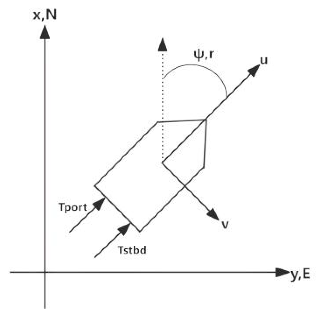
For USV trajectory tracking, three–degree–of–freedom (3–DOF) kinematic and dynamic models are typically formulated and analyzed. For notation, we adopt the convention introduced by Fossen [28]. The controlled vessel is a waterjet propulsion vessel with fixed thruster vector angles [29]. An illustration of the vessel in the inertial and body-fixed reference frames is provided in Figure 1.

The USV model comprises two parts [29]. The first relates the 3–DOF control inputs—surge force, sway force, and yaw moment—to the dynamics governing the vessel’s velocities, and can be written as:

$$\mathit{\tau }=\mathbf{M}\dot{\mathit{\nu }}+\mathbf{C}\left(\mathit{\nu }\right)\mathit{\nu }+\mathbf{D}\left(\mathit{\nu }\right)\mathit{\nu },$$

(1)

where $\mathit{\tau }$ is a vector of forces and moments generated by the port and starboard thrusters:

$$\mathit{\tau }=\left[\begin{array}{c}{\tau }_x\\ {\tau }_y\\ {\tau }_z\end{array}\right]=\left[\begin{array}{c}{\tau }_{\mathrm{port}}+{\tau }_{\mathrm{stbd}}\\ 0\\ \left({\tau }_{\mathrm{port}}-{\tau }_{\mathrm{stbd}}\right){\displaystyle \frac{B}{2}}\end{array}\right].$$

(2)

$\mathbf{M}$ is the inertia matrix, comprising the vessel mass, moments of inertia, and added–mass terms, and it characterizes the inertial properties during acceleration. $\mathbf{M}$ is denoted by:

$$\mathbf{M}=\left[\begin{array}{ccc}m-X_{\dot{u}}& 0& -m{y}_G\\ 0& m-Y_{\dot{v}}& m{x}_G-Y_{\dot{r}}\\ -m{y}_G& m{x}_G-N_{\dot{v}}& I_z-N_{\dot{r}}\end{array}\right].$$

(3)

The Coriolis matrix $\mathbf{C}\left(\mathit{\nu }\right)$ captures the coupling between inertia and velocity; it is typically skew-symmetric and accounts for Coriolis and centripetal effects during motion. $\mathbf{C}\left(\mathit{\nu }\right)$ is expressed as:

$$\begin{array}{cc}\hfill \mathbf{C}\left(\mathit{\nu }\right)& =\left[\begin{array}{ccc}0& 0& -m(x_{G}r+v)\\ 0& 0& -m(y_{G}r-u)\\ m(x_{G}r+v)& m(y_{G}r-u)& 0\end{array}\right]+\hfill \\ \hfill & \left[\begin{array}{ccc}0& 0& 2\left(Y_{\dot{v}}v+{\displaystyle \frac{Y_{\dot{r}}+N_{\dot{v}}}{2}}r\right)\\ 0& 0& -X_{\dot{u}}u\\ 2\left(-Y_{\dot{v}}v-{\displaystyle \frac{Y_{\dot{r}}+N_{\dot{v}}}{2}}r\right)& X_{\dot{u}}u& 0\end{array}\right].\hfill \end{array}$$

(4)

The damping matrix $\mathbf{D}\left(\mathit{\nu }\right)$ describes the influence of fluid damping and frictional losses on the vessel’s motion and usually contains both linear and nonlinear components. $\mathbf{D}\left(\mathit{\nu }\right)$ is denoted by:

$$\mathbf{D}\left(\mathit{\nu }\right)=-\left[\begin{array}{ccc}{X}_u& 0& 0\\ 0& Y_v& Y_r\\ 0& N_v& N_r\end{array}\right]-\left[\begin{array}{ccc}{X}_{u\left|u\right|}\left|u\right|& 0& 0\\ 0& Y_{v\left|v\right|}\left|v\right|+Y_{v\left|r\right|}\left|r\right|& Y_{r\left|v\right|}\left|v\right|+Y_{r\left|r\right|}\left|r\right|\\ 0& N_{v\left|v\right|}\left|v\right|+N_{v\left|r\right|}\left|r\right|& N_{r\left|v\right|}\left|v\right|+N_{r\left|r\right|}\left|r\right|\end{array}\right].$$

(5)

The velocity vector $\mathit{\nu }={[u,v,r]}^{\top }$ denotes, in the body-fixed reference frame, the surge and sway linear velocities and the yaw rate with physical units $u,v\in \mathrm{m}/\mathrm{s}$ and $r\in \mathrm{rad}/\mathrm{s}$, respectively.

The second part of the model describes the kinematic mapping between the body-fixed and inertial reference frames, transforming body-fixed velocities into the time derivatives of the inertial-frame pose, and is given by:

$$\dot{\mathit{\eta }}=\mathbf{J}\left(\mathit{\eta }\right)\mathit{\nu },$$

(6)

where $\mathit{\eta }={[x,y,\psi ]}^{\top }$ denotes the position and heading in the inertial reference frame, and $\mathbf{J}\left(\mathit{\eta }\right)$ is the coordinate transformation matrix that maps velocity vectors between the body-fixed and inertial reference frames:

$$\mathbf{J}\left(\mathit{\eta }\right)=\left[\begin{array}{ccc}cos\psi & -sin\psi & 0\\ sin\psi & cos\psi & 0\\ 0& 0& 1\end{array}\right].$$

(7)

The kinematic relations are formulated in an East–North–Up (ENU) right–handed inertial reference frame. Therefore, $\psi >0$ corresponds to a counterclockwise rotation in the horizontal plane.

In the vessel’s dynamic model, the values of certain elements in $\mathbf{M}$, $\mathbf{C}\left(\mathit{\nu }\right)$ and $\mathbf{D}\left(\mathit{\nu }\right)$ are determined by the vessel’s structural configuration. Moreover, the entries of $\mathbf{C}\left(\mathit{\nu }\right)$ and $\mathbf{D}\left(\mathit{\nu }\right)$ are velocity-dependent, and considerable parameter uncertainty is exhibited [30].

In this study, the specific values of the aforementioned parameters and the identification methods can be found in [1]. This USV dynamic model provides the foundational basis for the entire control system; subsequent controller design and simulation experiments are conducted on this model.

3. Control Scheme Design

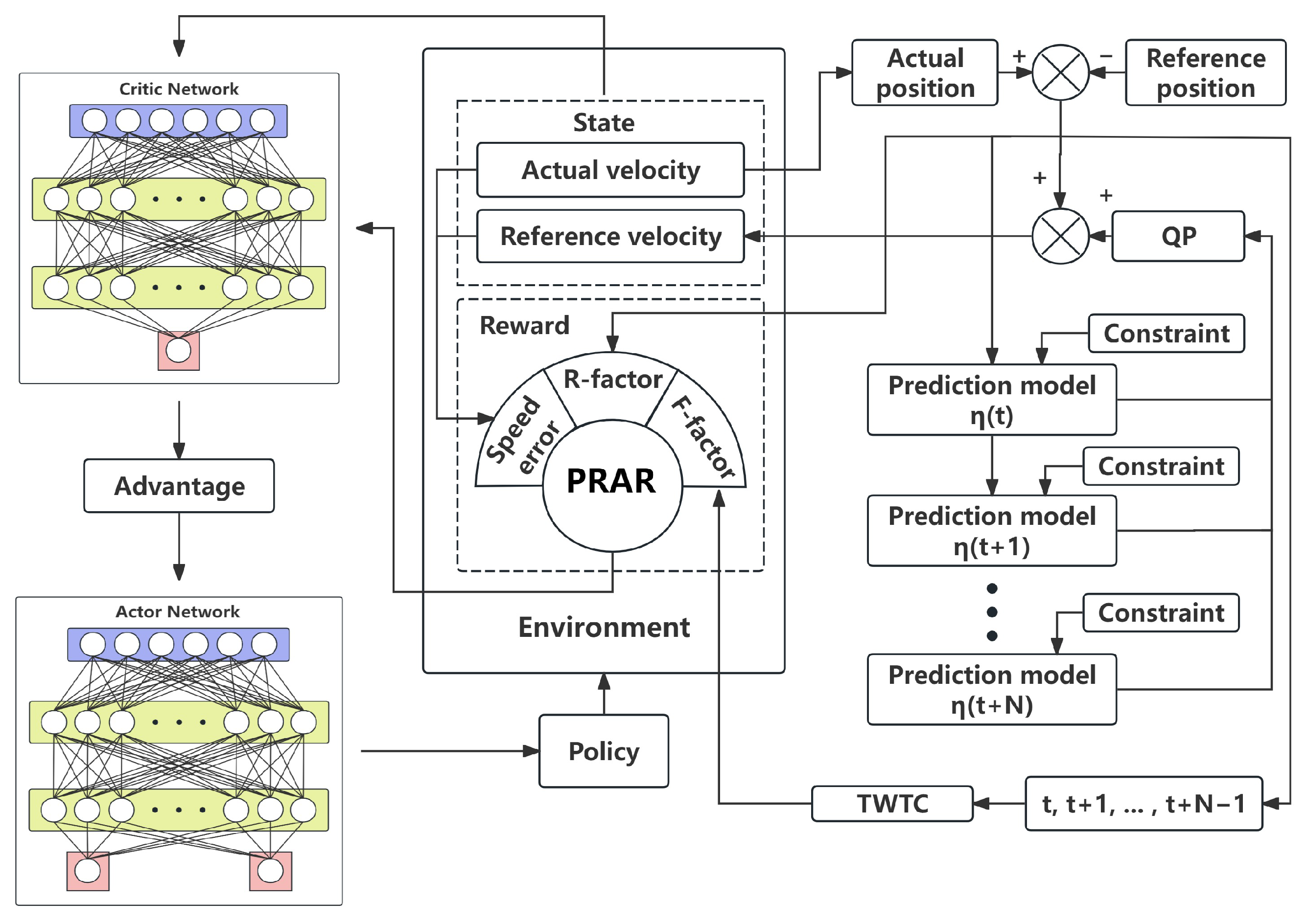
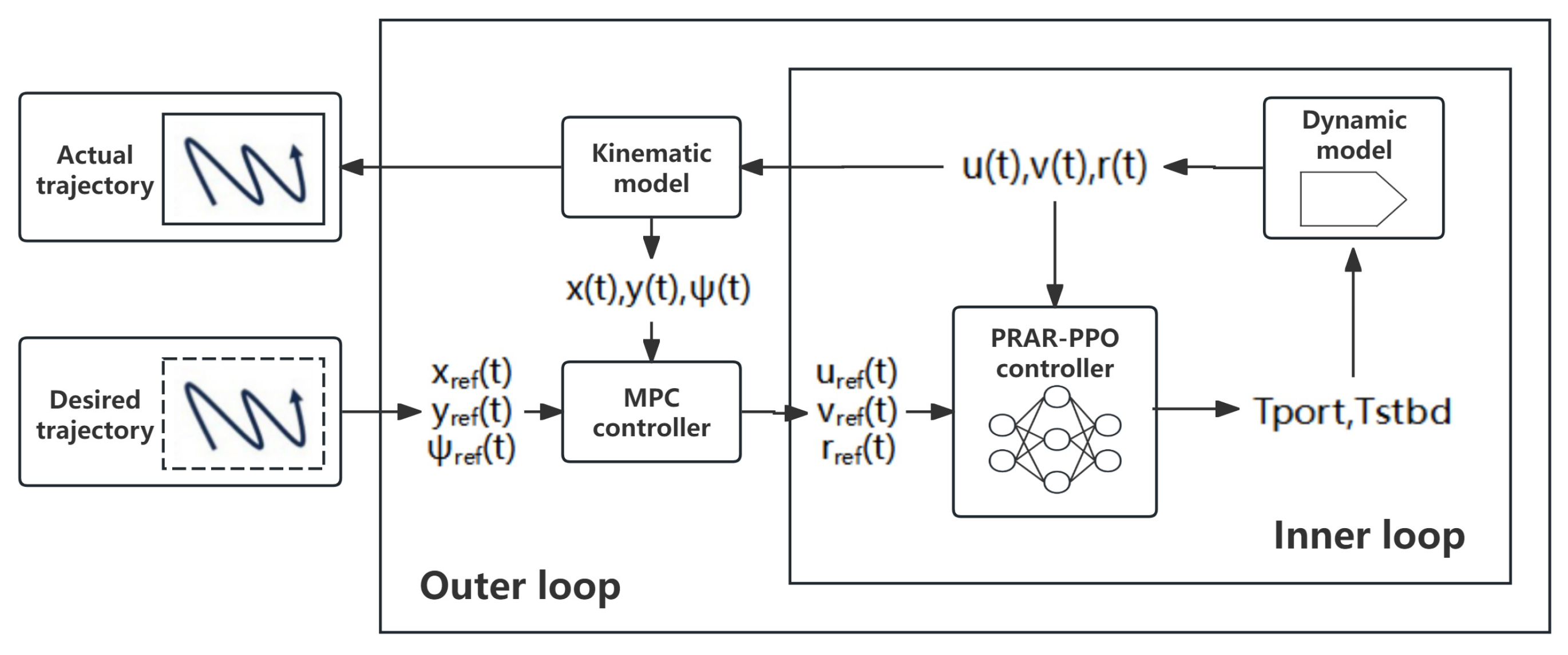
To achieve improved tracking performance, the complex USV trajectory-tracking task is decoupled into high–level kinematic planning combined with low–level dynamic control within a hierarchical framework. In this framework, the outer–loop controller performs long–horizon path planning in the inertial reference frame based on a concise and accurate kinematic model and generates the desired velocity commands. The inner–loop controller then addresses the more intricate and uncertain dynamic mapping, compensating model uncertainties and external disturbances through learning. The control architecture is shown in Figure 2.

In the outer loop, MPC algorithm is applied. Its model-based, long-horizon prediction capability is leveraged to compute optimal reference velocities on the basis of the vessel’s kinematic model, thereby achieving path planning. In the inner loop, a PPO–based agent is deployed. Its model-free, data-driven nature is exploited to learn to execute the MPC–issued commands accurately under complex nonlinear dynamics and unknown disturbances. Further details are provided in this section.

3.1. Outer–Loop Controller Based on MPC

The core task of the outer–loop controller is to generate, via online optimization, the optimal desired velocities in the body–fixed reference frame $(u_{\mathrm{ref}},v_{\mathrm{ref}},r_{\mathrm{ref}})$ based on the deviation between the vessel’s current state and the reference trajectory. These commands are then provided as references to the inner–loop PPO agent for execution.

The MPC–based outer–loop controller is built upon a mathematical model capable of accurately predicting the system’s future evolution, namely the kinematic model of the controlled USV introduced in the preceding section [29]:

$$\dot{\mathit{\eta }}=\left(\begin{array}{c}\dot{x}\\ \dot{y}\\ \dot{\psi }\end{array}\right)=\left(\begin{array}{ccc}cos\psi & -sin\psi & 0\\ sin\psi & cos\psi & 0\\ 0& 0& 1\end{array}\right)\left(\begin{array}{c}u\\ v\\ r\end{array}\right)=\mathbf{J}\left(\mathit{\eta }\right)\mathit{\nu }.$$

(8)

At each sampling instant k, a first–order Taylor expansion of Equation (8) is performed about the reference point $\left({\mathit{\eta }}_{\mathrm{ref},k},{\mathit{\nu }}_{\mathrm{ref},k}\right)$, yielding:

$$\Delta \dot{\mathit{\eta }}\approx {\mathbf{A}}_c\Delta \mathit{\eta }+{\mathbf{B}}_c\Delta \mathit{\nu },$$

(9)

where the Jacobian matrices ${\mathbf{A}}_c$ and ${\mathbf{B}}_c$ are given by:

$${\mathbf{A}}_c={\left.{\displaystyle \frac{\partial \left(\mathbf{J}\left(\mathit{\eta }\right)\mathit{\nu }\right)}{\partial \mathit{\eta }}}\right|}_{{\mathit{\eta }}_{\mathrm{ref}},{\mathit{\nu }}_{\mathrm{ref}}}=\left(\begin{array}{ccc}0& 0& -u_{\mathrm{ref}}sin{\psi }_{\mathrm{ref}}-v_{\mathrm{ref}}cos{\psi }_{\mathrm{ref}}\\ 0& 0& u_{\mathrm{ref}}cos{\psi }_{\mathrm{ref}}-v_{\mathrm{ref}}sin{\psi }_{\mathrm{ref}}\\ 0& 0& 0\end{array}\right),$$

(10)

$${\mathbf{B}}_c={\left.{\displaystyle \frac{\partial \left(\mathbf{J}\left(\mathit{\eta }\right)\mathit{\nu }\right)}{\partial \mathit{\nu }}}\right|}_{{\mathit{\eta }}_{\mathrm{ref}},{\mathit{\nu }}_{\mathrm{ref}}}=\left(\begin{array}{ccc}cos{\psi }_{\mathrm{ref}}& -sin{\psi }_{\mathrm{ref}}& 0\\ sin{\psi }_{\mathrm{ref}}& cos{\psi }_{\mathrm{ref}}& 0\\ 0& 0& 1\end{array}\right).$$

(11)

After forward Euler discretization, the discrete–time state–space representation is obtained as Equation (12):

$${\mathit{\eta }}_{k+1}=\left(\mathbf{I}+T{\mathbf{A}}_c\right){\mathit{\eta }}_k+\left(T{\mathbf{B}}_c\right){\mathit{\nu }}_k={\mathbf{A}}_{1,k}{\mathit{\eta }}_k+{\mathbf{B}}_{1,k}{\mathit{\nu }}_k,$$

(12)

where T denotes the sampling period and is set to $T=0.03s$. Accordingly, at sampling instant k, ${\mathbf{A}}_1$ and ${\mathbf{B}}_1$ can be derived as:

$$A_{1,k}=\left(\begin{array}{ccc}1& 0& T\left(-u_{\mathrm{ref}}sin{\psi }_{\mathrm{ref}}-v_{\mathrm{ref}}cos{\psi }_{\mathrm{ref}}\right)\\ 0& 1& T\left(u_{\mathrm{ref}}cos{\psi }_{\mathrm{ref}}-v_{\mathrm{ref}}sin{\psi }_{\mathrm{ref}}\right)\\ 0& 0& 1\end{array}\right),$$

(13)

$$B_{1,k}=\left(\begin{array}{ccc}Tcos{\psi }_{\mathrm{ref}}& -Tsin{\psi }_{\mathrm{ref}}& 0\\ Tsin{\psi }_{\mathrm{ref}}& Tcos{\psi }_{\mathrm{ref}}& 0\\ 0& 0& T\end{array}\right).$$

(14)

To obtain the complete state and control sequences over a prediction horizon $N_p=40$ and a control horizon $N_c=10$, and to compute the optimum of the cost function J, an augmented state ${\mathit{\xi }}_k\in {\mathbb{R}}^6$ is constructed:

$${\mathit{\xi }}_k=\left[\begin{array}{c}{\mathit{\eta }}_k-{\mathit{\eta }}_{\mathrm{ref},k}\\ {\mathit{\nu }}_{k-1}\end{array}\right],$$

(15)

where ${\mathit{\eta }}_k$ denotes the actual pose (position and heading) of the vessel at sampling instant k; ${\mathit{\eta }}_{\mathrm{ref},k}$ denotes the reference pose at the same instant; $v_{k-1}={[u_{k-1},v_{k-1},r_{k-1}]}^{\top }$ denotes the actual control output at the previous instant, namely the velocity commands in the three degrees of freedom. The control increment is defined as $\Delta v_k=v_k-v_{k-1}$. Accordingly, the update equations for the control state and the pose error can be obtained as:

$${\mathit{\nu }}_k=\mathbf{0}{\mathit{\eta }}_k+\mathbf{I}{\mathit{\nu }}_{k-1}+\mathbf{I}\Delta {\mathit{\nu }}_k,$$

(16)

$$\begin{array}{cc}\hfill {\mathit{\eta }}_{k+1}-{\mathit{\eta }}_{\mathrm{ref},k+1}& =\left({\mathbf{A}}_{1,k}{\mathit{\eta }}_k+{\mathbf{B}}_{1,k}{\mathit{\nu }}_k\right)-{\mathit{\eta }}_{\mathrm{ref},k+1}\hfill \\ \hfill & ={\mathbf{A}}_{1,k}\left({\mathit{\eta }}_k-{\mathit{\eta }}_{\mathrm{ref},k}\right)+{\mathbf{B}}_{1,k}\left({\mathit{\nu }}_{k-1}+\Delta {\mathit{\nu }}_k\right)+\left({\mathbf{A}}_{1,k}{\mathit{\eta }}_{\mathrm{ref},k}-{\mathit{\eta }}_{\mathrm{ref},k+1}\right).\hfill \end{array}$$

(17)

To simplify the model, the reference trajectory is assumed to vary slowly, so that the last term in the pose-error state update satisfies

$$\left({\mathbf{A}}_{1,k}{\mathit{\eta }}_{\mathrm{ref},k}-{\mathit{\eta }}_{\mathrm{ref},k+1}\right)\approx 0,$$

(18)

and the update can be approximated by

$${\mathit{\eta }}_{k+1}-{\mathit{\eta }}_{\mathrm{ref},k+1}={\mathbf{A}}_{1,k}\left({\mathit{\eta }}_k-{\mathit{\eta }}_{\mathrm{ref},k}\right)+{\mathbf{B}}_{1,k}\left({\mathit{\nu }}_{k-1}+\Delta {\mathit{\nu }}_k\right).$$

(19)

By combining the update of the control state with the pose–error update, the augmented state update can be derived as follows:

$${\mathit{\xi }}_{k+1}=\left[\begin{array}{c}{\mathit{\eta }}_{k+1}-{\mathit{\eta }}_{\mathrm{ref},k+1}\\ {\mathit{\nu }}_k\end{array}\right]=\left[\begin{array}{cc}{\mathbf{A}}_{1,k}& {\mathbf{B}}_{1,k}\\ {\mathbf{0}}_{3\times 3}& {\mathbf{I}}_{3\times 3}\end{array}\right]\left[\begin{array}{c}{\mathit{\eta }}_k-{\mathit{\eta }}_{\mathrm{ref},k}\\ {\mathit{\nu }}_{k-1}\end{array}\right]+\left[\begin{array}{c}{\mathbf{B}}_{1,k}\\ {\mathbf{I}}_{3\times 3}\end{array}\right]\Delta {\mathit{\nu }}_k,$$

(20)

and the augmented predictive model with the control increment $\Delta {\mathit{\nu }}_k$ as input can be obtained as:

$${\mathit{\xi }}_{k+1}={\mathbf{A}}_k{\mathit{\xi }}_k+{\mathbf{B}}_k\Delta {\mathit{\nu }}_k,$$

(21)

where

$${\mathbf{A}}_k=\left(\begin{array}{cc}{\mathbf{A}}_{1,k}& {\mathbf{B}}_{1,k}\\ {\mathbf{0}}_{3\times 3}& {\mathbf{I}}_{3\times 3}\end{array}\right),{\mathbf{B}}_k=\left(\begin{array}{c}{\mathbf{B}}_{1,k}\\ {\mathbf{I}}_{3\times 3}\end{array}\right).$$

(22)

This predictive model clearly characterizes the dynamic evolution of the pose error at the current instant and the previous control input under the action of the control increment. To extract the internal pose from the augmented state for subsequent prediction and weighting in the cost function, we use an output matrix $\mathbf{C}\in {\mathbb{R}}^{3\times 6}$:

$$\mathbf{C}=\left[{\mathbf{I}}_{3\times 3}{\mathbf{0}}_{3\times 3}\right]=\left(\begin{array}{cccccc}1& 0& 0& 0& 0& 0\\ 0& 1& 0& 0& 0& 0\\ 0& 0& 1& 0& 0& 0\end{array}\right),$$

(23)

and map the augmented error state ${\mathit{\xi }}_k$ to the output ${\mathbf{e}}_k$:

$${\mathbf{e}}_k=\mathbf{C}{\mathit{\xi }}_k={\mathit{\eta }}_k-{\mathit{\eta }}_{\mathrm{ref},k}.$$

(24)

By iterating the predictive model in Equation (21), a relationship is established between the future states over the prediction horizon $N_p$, the current augmented state ${\mathit{\xi }}_k$, and the sequence of control increments over the control horizon $N_c$[31]. At time step k, the one–step–ahead prediction for the next sampling instant is defined as:

$${\mathit{\xi }}_{k+1|k}={\mathbf{A}}_k{\mathit{\xi }}_k+{\mathbf{B}}_k\Delta {\mathit{\nu }}_k.$$

(25)

The two–step–ahead prediction at time step $k+2$ is defined as:

$${\mathit{\xi }}_{k+2|k}={\mathbf{A}}_k{\mathit{\xi }}_{k+1|k}+{\mathbf{B}}_k\Delta {\mathit{\nu }}_{k+1}.$$

(26)

Substituting the expression of ${\mathit{\xi }}_{k+1\mid k}$ into the above yields the relationship between the current state ${\mathit{\xi }}_k$ and the two–step–ahead prediction ${\mathit{\xi }}_{k+2\mid k}$:

$${\mathit{\xi }}_{k+2|k}={\mathbf{A}}_k\left({\mathbf{A}}_k{\mathit{\xi }}_k+{\mathbf{B}}_k\Delta {\mathit{\nu }}_k\right)+{\mathbf{B}}_k\Delta {\mathit{\nu }}_{k+1}={\mathbf{A}}_k^2{\mathit{\xi }}_k+{\mathbf{A}}_k{\mathbf{B}}_k\Delta {\mathit{\nu }}_k+{\mathbf{B}}_k\Delta {\mathit{\nu }}_{k+1}.$$

(27)

By induction, the i–step–ahead prediction at time step k is derived as:

$${\mathit{\xi }}_{k+i|k}={\mathbf{A}}_k^i{\mathit{\xi }}_k+\sum _{j=0}^{i-1}{\mathbf{A}}_k^{i-1-j}{\mathbf{B}}_k\Delta {\mathit{\nu }}_{k+j}.$$

(28)

Stack all predicted state vectors from $i=1$ to $N_p$ into a long vector ${\mathbf{\Xi }}_k$:

$${\mathbf{\Xi }}_k=\left[\begin{array}{c}{\mathit{\xi }}_{k+1|k}\\ {\mathit{\xi }}_{k+2|k}\\ ⋮\\ {\mathit{\xi }}_{k+N_p|k}\end{array}\right].$$

(29)

Stack all control increments from $j=0$ to $N_c-1$ into another column vector:

$$\Delta {\mathbf{U}}_k=\left[\begin{array}{c}\Delta {\mathit{\nu }}_k\\ \Delta {\mathit{\nu }}_{k+1}\\ ⋮\\ \Delta {\mathit{\nu }}_{k+N_c-1}\end{array}\right].$$

(30)

Then the state prediction equation can be derived as:

$${\mathbf{\Xi }}_k={\mathbf{\Phi }}_k{\mathit{\xi }}_k+{\mathbf{\Theta }}_k\Delta {\mathbf{U}}_k,$$

(31)

where the prediction matrices ${\mathbf{\Phi }}_k$ and ${\mathbf{\Theta }}_k$ are given by:

$${\mathbf{\Phi }}_k=\left[\begin{array}{c}{\mathbf{A}}_k\\ {\mathbf{A}}_k^2\\ ⋮\\ {\mathbf{A}}_k^{N_p}\end{array}\right],{\mathbf{\Theta }}_k=\left(\begin{array}{cccc}{\mathbf{B}}_k& \mathbf{0}& \dots & \mathbf{0}\\ {\mathbf{A}}_k{\mathbf{B}}_k& {\mathbf{B}}_k& \dots & \mathbf{0}\\ ⋮& ⋮& \ddots & ⋮\\ {\mathbf{A}}_k^{N_p-1}{\mathbf{B}}_k& {\mathbf{A}}_k^{N_p-2}{\mathbf{B}}_k& \dots & {\mathbf{A}}_k^{N_p-N_c}{\mathbf{B}}_k\end{array}\right).$$

(32)

Since the cost function acts directly on the output ${\mathit{e}}_k$, the prediction equation is combined with the pose-error output equation to obtain the predicted output sequence over $N_p$ steps, denoted by:

$${\mathbf{E}}_k=diag(\underset{N_p}{\underbrace{\mathbf{C},\dots ,\mathbf{C}}}){\mathbf{\Xi }}_k=\tilde{\mathbf{C}}\left({\mathbf{\Phi }}_k{\mathit{\xi }}_k+{\mathbf{\Theta }}_k\Delta {\mathbf{U}}_k\right),$$

(33)

where $\tilde{\mathbf{C}}$ is the block–diagonal output matrix. For notational simplicity, the prediction relation is rewritten as:

$${\mathbf{E}}_k=\mathbf{\Phi }{\mathit{\xi }}_k+\mathbf{\Theta }\Delta {\mathbf{U}}_k,$$

(34)

and the prediction matrices $\mathbf{\Phi }$ and $\mathbf{\Theta }$ are redefined as:

$$\mathbf{\Phi }=\left[\begin{array}{c}\mathbf{C}{\mathbf{A}}_k\\ \mathbf{C}{\mathbf{A}}_k^2\\ ⋮\\ \mathbf{C}{\mathbf{A}}_k^{N_p}\end{array}\right],\mathbf{\Theta }=\left(\begin{array}{cccc}\mathbf{C}{\mathbf{B}}_k& \mathbf{0}& \dots & \mathbf{0}\\ \mathbf{C}{\mathbf{A}}_k{\mathbf{B}}_k& \mathbf{C}{\mathbf{B}}_k& \dots & \mathbf{0}\\ ⋮& ⋮& \ddots & ⋮\\ \mathbf{C}{\mathbf{A}}_k^{N_p-1}{\mathbf{B}}_k& \mathbf{C}{\mathbf{A}}_k^{N_p-2}{\mathbf{B}}_k& \dots & \mathbf{C}{\mathbf{A}}_k^{N_p-N_c}{\mathbf{B}}_k\end{array}\right).$$

(35)

At each control period, the MPC controller solves a finite–horizon optimization problem formulated as a standard quadratic program. The cost function J is defined as:

$$J(\Delta {\mathbf{U}}_k,s)=\sum _{i=1}^{N_p}{∥{\mathbf{e}}_{k+i|k}∥}_{\mathbf{Q}}^2+\sum _{j=0}^{N_c-1}{∥\Delta {\mathit{\nu }}_{k+j|k}∥}_{\mathbf{R}}^2+\rho s^2,$$

(36)

where $\mathbf{Q}$ and $\mathbf{R}$ denote the weighting matrices for the tracking error and the control increment, respectively, and are chosen as constant diagonal matrices with $\mathbf{Q}=diag(100,100,150)$ and $\mathbf{R}=diag(0.5,0.5,3)$. s is a slack variable, and $\rho >0$ is its penalty coefficient. By substituting the prediction Equation (34) into the cost function Equation (36) and introducing the slack variable s, the optimization is reformulated as a quadratic program (QP). Let the optimization variable be defined as:

$$\mathbf{z}=\left[\begin{array}{c}\Delta {\mathbf{U}}_k\\ s\end{array}\right].$$

(37)

Then the original optimization problem can be expressed in the standard QP objective form as:

$$\underset{\mathbf{z}}{min}J\left(\mathbf{z}\right)=\frac{1}{2}{\mathbf{z}}^{\top }\mathbf{H}\mathbf{z}+{\mathit{f}}^{\top }\mathbf{z}.$$

(38)

The Hessian matrix $\mathbf{H}$ and the gradient vector $\mathit{f}$ are derived from the cost function Equation (36):

$$\mathbf{H}=\left(\begin{array}{cc}2\left({\mathbf{\Theta }}^{\top }\tilde{\mathbf{Q}}\mathbf{\Theta }+\tilde{\mathbf{R}}\right)& \mathbf{0}\\ \mathbf{0}& 2\rho \end{array}\right),$$

(39)

$$\mathit{f}=\left(\begin{array}{c}2{\mathbf{\Theta }}^{\top }\tilde{\mathbf{Q}}\mathbf{\Phi }{\mathit{\xi }}_k\\ 0\end{array}\right),$$

(40)

where $\tilde{\mathbf{Q}}=diag(\mathbf{Q},\dots ,\mathbf{Q})$ and $\tilde{\mathbf{R}}=diag(\mathbf{R},\dots ,\mathbf{R})$ are the block–diagonal weighting matrices expanded over the entire horizon.

The optimization must also satisfy physical constraints. In this work, amplitude constraints are imposed on both the control inputs and the control increments:

$$\left\{\begin{array}{cc}\hfill {\mathit{\nu }}_{\min }& \le {\mathit{\nu }}_k\le {\mathit{\nu }}_{\max }\hfill \\ \hfill \Delta {\mathit{\nu }}_{\min }& \le \Delta {\mathit{\nu }}_k\le \Delta {\mathit{\nu }}_{\max }\hfill \end{array}\right.$$

(41)

These constraints are converted into linear inequality constraints on the decision variable $\mathit{z}$. At each sampling step k, the quadratic program is solved online. The first element of the optimal control–increment sequence, $\Delta {\mathit{\nu }}_k^{\ast }$, is then used to update the current control input:

$${\mathit{\nu }}_k={\mathit{\nu }}_{k-1}+\Delta {\mathit{\nu }}_k^{★}.$$

(42)

The final controller output is the sum of the feedback control input and the feedforward velocity, which is then supplied as the reference signal to the inner–loop PPO controller.

3.2. Inner–Loop Controller Based on PRAR–PPO

The inner loop adopts PRAR–enhanced PPO.This closed–loop controller focuses solely on learning the inverse dynamic mapping from velocity to thrust within the volume coordinate system, thereby achieving precise tracking of the velocity commands output by the outer-loop MPC controller.

3.2.1. PPO

PPO is an on-policy Actor–Critic algorithm. Its key innovation is the introduction of a clipped surrogate objective function, which mitigates destructive policy degradation caused by excessively large update steps in traditional policy-gradient methods [32].

To quantify and effectively constrain the discrepancy between the new and old policies during updates, PPO defines a probability ratio:

$$r_t\left(\theta \right)={\displaystyle \frac{{\pi }_{\theta }(a_t\mid s_t)}{{\pi }_{{\theta }_{\mathrm{old}}}(a_t\mid s_t)}},$$

(43)

where ${\pi }_{\theta }$ denotes the policy with the current trainable parameters, while ${\pi }_{{\theta }_{\mathrm{old}}}$ denotes the behavior policy used to interact with the environment and collect data. If $r_t\left(\theta \right)>1$,the new policy increases the probability of taking action $a_t$ in state $s_t$; conversely, if $r_t\left(\theta \right)<1$, the new policy decreases that probability.

In the PPO algorithm, the advantage function $A_t$ evaluates how good the current action is in the current state:

$$A_t=\sum _{l=0}^{\infty }{\left(\gamma \lambda \right)}^l{\delta }_{t+l},$$

(44)

where $\gamma$ is the discount factor; $\lambda$ is the coefficient controlling the bias in advantage estimation; and ${\delta }_t$ is the temporal-difference error. The specific form of ${\delta }_t$ is given by:

$${\delta }_t=r_t+\gamma V\left(s_{t+1}\right)-V\left(s_t\right),$$

(45)

where $V\left(s_t\right)$ and $V\left(s_{t+1}\right)$ denote the state values at the current state $s_t$ and the next state $s_{t+1}$.

Using the above equations, we compute the advantage estimate $A_t$ at each sampling time. Unlike standard policy–gradient objectives, PPO adopts a clipped surrogate objective: by introducing a clipping mechanism to constrain $r_t\left(\theta \right)$, it suppresses overly aggressive policy updates. The final optimization objective is given in Equation (46):

$$L^{\mathrm{CLIP}}\left(\theta \right)={\mathbb{E}}_t\left[min\left(r_t\left(\theta \right)A_t,clip\left(r_t\left(\theta \right),1-ϵ,1+ϵ\right)A_t\right)\right],$$

(46)

where $ϵ=0.1$ is the clipping width. This clipping operation constrains $r_t\left(\theta \right)$ to the interval $[1-ϵ,1+ϵ]$, thereby ensuring stable updates.

By formulating and optimizing the clipped surrogate objective, PPO strictly constrains the magnitude of policy updates, thereby achieving more effective learning while preserving stability.

3.2.2. State and Action Space

(1)

State Space

The state space of the inner-loop controller aims to comprehensively represent the state information of the USV dynamics model. Higher-level trajectory-planning states (e.g., pose error) are fully decoupled and handled by the outer-loop MPC; only the velocity command is fed into the inner-loop agent’s state space. Since the input of the inner loop is the reference velocity command from the outer loop, and the output is the actual velocity output by the dynamics model, we define the state space s as a direct combination of these two vectors, as given by Equation (47):

$$\mathit{s}={\left[{\mathit{\nu }}_{\mathrm{ref}}{\left(t\right)}^{\top },{\mathit{\nu }}_{\mathrm{actual}}{\left(t\right)}^{\top }\right]}^{\top },$$

(47)

where ${\mathit{\nu }}_{\mathrm{ref}}\left(t\right)={[u_{\mathrm{ref}}\left(t\right),v_{\mathrm{ref}}\left(t\right),r_{\mathrm{ref}}\left(t\right)]}^{\top }$ denotes the desired velocity command passed from the outer loop to the inner loop, and ${\mathit{\nu }}_{\mathrm{actual}}\left(t\right)={[u_{\mathrm{actual}}\left(t\right),v_{\mathrm{actual}}\left(t\right),r_{\mathrm{actual}}\left(t\right)]}^{\top }$ denotes the actual velocity produced by the inner loop; all components are measured in $\mathrm{m}/\mathrm{s}$.

(2)

Action Space

The agent’s action space $\mathbf{a}$ corresponds to the control inputs of the USV dynamics model, namely the thrust commands applied to the two thrusters, and is defined as:

$$\mathbf{a}={\left[T_{\mathrm{port}},T_{\mathrm{stbd}}\right]}^{\top },$$

(48)

where $T_{\mathrm{port}}$ and $T_{\mathrm{stbd}}$ denote the control commands for the port–side and starboard–side thrusters, respectively. Subject to the thrusters’ physical capability limits, the command range is normalized to $[0,10]$. In the simulation environment, this command is linearly mapped via a gain block to the actual physical thrust range $[0\mathrm{N},2000\mathrm{N}]$.

3.2.3. PRAR

In reinforcement learning, the design of the reward function is crucial to both learning efficiency and the final performance of the policy. A reasonable reward function can transform high–level control objectives into specific, optimizable numerical signals. The static reward function commonly used in the standard PPO algorithm is typically designed as a secondary penalty for tracking error, using a fixed set of weight coefficients:

$$r_t=-\left(w_u{e}_u{\left(t\right)}^2+w_v{e}_v{\left(t\right)}^2+w_r{e}_r{\left(t\right)}^2\right),$$

(49)

where $e_u\left(t\right),e_v\left(t\right),e_r\left(t\right)$ denote the velocity errors in surge, sway, and yaw rate, respectively, and $w_u,w_v,w_r$ are manually tuned weighting hyperparameters. Such a fixed reward function may not fully accommodate the diverse learning needs across different training stages [33]. Because the reward is computed purely from historical errors, the agent receives negative feedback only after the error has already occurred and begun to accumulate; as a result, the penalty mechanism cannot proactively guide the controller to anticipate imminent disturbances and trajectory deviations, nor to adjust and guard against them in time—leading to a pronounced response lag.

To overcome these limitations, we leverage the characteristics of the outer–loop MPC and design a Proactive–Reactive Adaptive Reward (PRAR) that uses both the pose–tracking error and the rolling prediction sequence generated by the MPC. This mechanism reflects real–time errors while accounting for the future task difficulty, as illustrated in Figure 3:

This method replaces the fixed penalty weights in the baseline reward with a dynamically computed, real-time weight vector $\mathbf{W}\left(t\right)$. The reward $r_t$ is defined as:

$$r_t=-\mathbf{e}{\left(t\right)}^{\top }diag\left(\mathbf{W}\left(t\right)\right)\mathbf{e}\left(t\right),$$

(50)

where $\mathbf{e}\left(t\right)={[e_u\left(t\right),e_v\left(t\right),e_r\left(t\right)]}^{\top }$ is the instantaneous velocity–tracking error vector, and $\mathbf{e}{\left(t\right)}^2$ denotes the element-wise square.

For the dynamic weight vector $\mathbf{W}\left(t\right)$, its computation is given by:

$$\mathbf{W}\left(t\right)={\mathbf{W}}_{\mathrm{base}}\odot {\mathit{f}}_{\mathrm{reactive}}\left(t\right)\odot {\mathit{f}}_{\mathrm{proactive}}\left(t\right),$$

(51)

where ⊙ denotes element–wise multiplication, ${\mathbf{W}}_{\mathrm{base}}$ is the baseline weight vector, and ${\mathit{f}}_{\mathrm{reactive}}\left(t\right)$ and ${\mathit{f}}_{\mathrm{proactive}}\left(t\right)$ are the reactive and predictive factors, respectively.

(1)

Reactive factor

To address the limited adaptivity of static rewards, a reactive factor is designed to enhance the controller’s responsiveness to the current tracking performance. This factor receives the desired pose $\mathit{\eta }={[x,y,\psi ]}^{\top }$ and the actual pose ${\mathit{\eta }}_{\mathrm{r}}={[x_{\mathrm{r}},y_{\mathrm{r}},{\psi }_{\mathrm{r}}]}^{\top }$ output by the outer-loop controller. The module then computes the instantaneous pose error:

$${\mathbf{e}}_p=\left[\begin{array}{c}{e}_x\\ e_y\end{array}\right]=\left[\begin{array}{c}x-x_r\\ y-y_r\end{array}\right],$$

(52)

$$e_{\psi }=atan2\left(sin(\psi -{\psi }_r),cos(\psi -{\psi }_r)\right),$$

(53)

where ${\mathbf{e}}_p$ denotes the position–error vector and $e_{\psi }$ denotes the heading–angle error. To directly apply the error extracted from the outer loop to the USV dynamic model, the error is transformed from the inertial reference frame to the body–fixed reference frame. This coordinate transformation is accomplished via the rotation matrix $\mathbf{R}\left(\psi \right)$ parameterized by the current heading:

$$\mathbf{R}\left(\psi \right)=\left[\begin{array}{cc}cos\psi & sin\psi \\ -sin\psi & cos\psi \end{array}\right].$$

(54)

By concatenating the decoupled longitudinal and lateral position errors with the heading error, a unified error vector $\mathit{e}\left(t\right)\in {\mathbb{R}}^3$ can be obtained:

$$\mathbf{e}\left(t\right)=\left[\begin{array}{c}{e}_u\left(t\right)\\ e_v\left(t\right)\\ e_{\psi }\left(t\right)\end{array}\right]=\left[\begin{array}{c}{e}_{x}cos\psi +e_{y}sin\psi \\ -e_{x}sin\psi +e_{y}cos\psi \\ e_{\psi }\end{array}\right].$$

(55)

Finally, the error vector $\mathbf{e}\left(t\right)$ is mapped, elementwise, by a nonlinear function to the weighting adjustment factors associated with each degree of freedom:

$$f_{\mathrm{reactive},i}\left(t\right)=1+A_r·\left(1-exp(-\alpha |e_i\left(t\right)\left|\right)\right),i\in \{u,v,r\},$$

(56)

where $e_i$ is the error for each channel, $A_r$ is the reactive amplitude, which specifies the upper bound on the gain provided by the reactive factor, and $\alpha$ is reactive sensitivity, by which the growth rate of the factor with increasing error magnitude is controlled.

The reactive factor performs a nonlinear, bounded, and smooth gain mapping of the pose error. As a result, when the vessel deviates from the planned course, the penalty on velocity–tracking error is promptly increased, enabling automatic adaptation to the current control task.

(2)

Proactive factor

To mitigate the response lag inherent in conventional reward functions that rely solely on historical information, the future velocity sequence generated by the outer–loop MPC during receding–horizon optimization is incorporated into the reward design [34]. And a predictive adjustment factor is devised consequently. This factor converts the MPC controller’s forecast of future task complexity into a feedforward modulation signal, thereby allowing the inner–loop agent to prepare in advance before pronounced changes in the control commands occur.

Through a dedicated module, the factor receives the velocity planning sequence over the next $N_p$ time steps generated by the outer-loop MPC:

$${\mathit{V}}_{\mathrm{ref}}\left(t\right)={\left[{\mathit{\nu }}_{u,0},{\mathit{\nu }}_{v,0},{\mathit{\nu }}_{r,0},\dots ,{\mathit{\nu }}_{u,N_p-1},{\mathit{\nu }}_{v,N_p-1},{\mathit{\nu }}_{r,N_p-1}\right]}^{\top }\in {\mathbb{R}}^{3N_p}.$$

(57)

It is then reshaped as:

$${\mathbf{V}}_{\mathrm{plan}}\left(t\right)=\left[\begin{array}{ccc}{\mathit{\nu }}_{u,0}& {\mathit{\nu }}_{v,0}& {\mathit{\nu }}_{r,0}\\ {\mathit{\nu }}_{u,1}& {\mathit{\nu }}_{v,1}& {\mathit{\nu }}_{r,1}\\ ⋮& ⋮& ⋮\\ {\mathit{\nu }}_{u,N_p-1}& {\mathit{\nu }}_{v,N_p-1}& {\mathit{\nu }}_{r,N_p-1}\end{array}\right]\in {\mathbb{R}}^{N_p\times 3},$$

(58)

where the k-th row gives the reference velocities for the k-th prediction step across the three channels. To emphasize the importance of near-term predictions for the current decision, a time–attention weight $w_k$ is defined:

$$w_k={\sigma }^k,k=0,\dots ,N_p-2,$$

(59)

where $\sigma$ is the temporal decay factor, which assigns weights to the complexity at future steps. Normalization yields:

$${\alpha }_k={\displaystyle \frac{w_k}{{\displaystyle \sum _{j=0}^{N_p-2}{w}_j}}},\sum _{k=0}^{N_p-2}{\alpha }_k=1.$$

(60)

Subsequently, a first-order difference is taken between adjacent samples for each channel:

$$\Delta {\nu }_{i,k+1}=|{\nu }_{i,k+1}-{\nu }_{i,k}|,k=0,\dots ,N_p-2.$$

(61)

Based on this definition, a time-weighted trajectory complexity (TWTC) metric is introduced to quantify the complexity of the planned velocity sequence:

$$C_{t,i}=\sum _{k=0}^{N_p-2}{\alpha }_k\left|{\nu }_{i,k+1}-{\nu }_{i,k}\right|,i\in \{u,v,r\}.$$

(62)

Segments in ${\mathit{V}}_{\mathrm{ref}}\left(t\right)$ that are closer to the present and exhibit sharper variations yield higher trajectory complexity. This design enables the agent to place greater emphasis on imminent and rapidly changing commands and their impact on policy stability.

After computing the trajectory complexity index for each channel, the hyperbolic tangent is employed as the activation function to map these indices to the final predictive adjustment factors:

$$f_{\mathrm{proactive},i}\left(t\right)=1+A_p·tanh\left(\beta ·C_{t,i}\right),$$

(63)

where $A_p$ is the proactive amplitude, which specifies the maximum gain attainable by the predictive adjustment factor, and $\beta$ is proactive sensitivity, by which the growth rate of the factor with increasing trajectory complexity is controlled.

By quantifying the dynamic complexity of the MPC’s future plan and mapping it nonlinearly into a bounded, smooth gain–modulation signal, the predictive adjustment factor is obtained. This factor enables the controller to increase the penalty on velocity–tracking error in advance when pronounced changes in future commands are anticipated, thereby achieving proactive anticipation and adaptive adjustment to forthcoming task challenges.

Collecting the above definitions, the mapping from the real–time pose error and the MPC–based trajectory complexity to the time-varying reward weights can be written in closed form. For each degree of freedom $i\in \{u,v,r\}$, the adaptive weight applied to the velocity–tracking error at time step k is given by:

$$\begin{array}{cc}\hfill W_i\left(k\right)& =W_{\mathrm{base},i}\left[1+A_r\left(1-{\mathrm{e}}^{-\alpha |e_i\left(k\right)|}\right)\right]\left[1+A_{p}tanh\left(\beta C_{k,i}\right)\right],\hfill \\ \hfill C_{k,i}& =\sum _{\ell =0}^{N_p-2}{\displaystyle \frac{{\sigma }^{\ell }}{{\displaystyle \sum _{j=0}^{N_p-2}{\sigma }^j}}}\left|{\nu }_{i,\ell +1}\left(k\right)-{\nu }_{i,\ell }\left(k\right)\right|.\hfill \end{array}$$

(64)

which shows that $W_i\left(k\right)$ increases monotonically with both the instantaneous pose error $|e_i\left(k\right)|$ and the predicted trajectory complexity $C_{k,i}$. The PRAR–weighted reward used by the inner–loop PPO controller is finally given by:

$$r_k=-\sum _{i\in \{u,v,r\}}{W}_i\left(k\right)e_{v,i}^2\left(k\right),$$

(65)

where $e_{v,i}\left(k\right)$ denotes the velocity–tracking error in surge, sway or yaw. In this way, PRAR provides an explicit, time–varying mapping from real–time pose errors and MPC–based complexity indices to the scalar penalty coefficients in the reinforcement–learning reward.

3.3. Implementation of PRAR–PPO

The complete implementation is summarized as Algorithm 1:

Algorithm 1 MPC–PRAR–PPO dual–loop control

Require: USV kinematic and dynamic models; prediction horizon $N_p$; control horizon $N_c$; sample time T;   1: input and rate constraints; PRAR parameters $(A_r,\alpha ,A_p,\beta ,\gamma )$;   2: policy ${\pi }_{\theta }$ and value function $V_{\varphi }$   3: Initialize previous reference velocity ${\nu }_{-1}^{\mathrm{ref}}\leftarrow \mathbf{0}$ and base weights $W_{\mathrm{base}}\leftarrow {[w_u,w_v,w_r]}^{\top }$   4: Set time index $k\leftarrow 0$   5: while mission not finished do   6:       Measure current pose ${\eta }_k={[x_k,y_k,{\psi }_k]}^{\top }$ and body–fixed velocity ${\nu }_k^{\mathrm{act}}={[u_k,v_k,r_k]}^{\top }$   7:       Obtain reference pose ${\eta }_k^{\mathrm{ref}}={[x_k^{\mathrm{ref}},y_k^{\mathrm{ref}},{\psi }_k^{\mathrm{ref}}]}^{\top }$ from path generator   8:       Form augmented state ${\xi }_k$ from pose error $({\eta }_k-{\eta }_k^{\mathrm{ref}})$ and the internally stored previous virtual input   9:       Linearize kinematic model, build MPC prediction matrices and quadratic program 10:       Solve MPC to obtain current reference velocity ${\nu }_k^{\mathrm{ref}}={[u_k^{\mathrm{ref}},v_k^{\mathrm{ref}},r_k^{\mathrm{ref}}]}^{\top }$ 11: and prediction sequence $V_{\mathrm{ref}}\left(k\right)\in {\mathbb{R}}^{3N_p}$ 12:       Compute inertial position errors $e_x=x_k-x_k^{\mathrm{ref}}$, $e_y=y_k-y_k^{\mathrm{ref}}$ 13:       Compute heading error $e_{\psi }=\mathrm{atan}2\left(sin({\psi }_k-{\psi }_k^{\mathrm{ref}}),cos({\psi }_k-{\psi }_k^{\mathrm{ref}})\right)$ 14:       Transform $(e_x,e_y)$ into body-fixed errors using ${\psi }_k$: 15: $e_u=e_{x}cos{\psi }_k+e_{y}sin{\psi }_k$, $e_v=-e_{x}sin{\psi }_k+e_{y}cos{\psi }_k$ 16:       Set $e\left(k\right)={[e_u,e_v,e_{\psi }]}^{\top }$ 17:       for $i\in \{u,v,r\}$ do 18:          Compute reactive factor $f_i^{\mathrm{react}}\left(k\right)=1+A_r\left(1-exp(-\alpha |e_i\left(k\right)\left|\right)\right)$ 19:       end for 20:       Reshape $V_{\mathrm{ref}}\left(k\right)$ into $V_{\mathrm{plan}}\left(k\right)\in {\mathbb{R}}^{N_p\times 3}$ and set ${\alpha }_{\ell }={\sigma }^{\ell }/{\sum }_{j=0}^{N_p-2}{\sigma }^j$ 21:       for $i\in \{u,v,r\}$ do 22:          Compute trajectory complexity $C_{k,i}={\sum }_{\ell =0}^{N_p-2}{\alpha }_{\ell }|{\nu }_{i,\ell +1}-{\nu }_{i,\ell }|$ 23:          Compute proactive factor $f_i^{\mathrm{pro}}\left(k\right)=1+A_{p}tanh\left(\beta C_{k,i}\right)$ 24:          Update adaptive weight $W_i\left(k\right)=W_{\mathrm{base},i}{f}_i^{\mathrm{react}}\left(k\right)f_i^{\mathrm{pro}}\left(k\right)$ 25:       end for 26:       Construct policy input $s_k={[{\left({\nu }_k^{\mathrm{ref}}\right)}^{\top },{\left({\nu }_k^{\mathrm{act}}\right)}^{\top }]}^{\top }\in {\mathbb{R}}^6$ 27:       Generate action $a_k={\pi }_{\theta }\left(s_k\right)$ (or sample from ${\pi }_{\theta }(·\mid s_k)$) and map it to thrust command ${\tau }_k$ 28:       Apply ${\tau }_k$ to the USV dynamics to obtain next pose ${\eta }_{k+1}$ and velocity ${\nu }_{k+1}^{\mathrm{act}}$ 29:       If learning is enabled then 30:          Compute reward $r_k$ from ${\nu }_k^{\mathrm{ref}}$, ${\nu }_k^{\mathrm{act}}$ and $W_i\left(k\right)$ 31:          Store transition $(s_k,a_k,r_k,s_{k+1})$ and update $\theta ,\varphi$ by PPO 32:       End if 33:       Set $k\leftarrow k+1$ 34: end while

4. Simulation Results and Analysis

To validate the effectiveness of the proposed PRAR–DLC scheme in USV trajectory tracking, five groups of comparative experiments are conducted: (1) a single–loop controller that relies solely on PPO; (2) a dual–loop architecture in which the outer-loop controller is retained while the inner loop is replaced with a carefully tuned PID controller based on the nominal hydrodynamic model; (3) a dual-loop MPC–PPO controller with fixed penalty weights; (4) an MPC–PPO controller incorporating only the Proactive factor; and (5) an MPC–PPO controller incorporating only the Reactive factor. This configuration enables a systematic assessment of how different reward designs influence the overall USV control performance.

The VTec S-III USV is selected as the controlled vessel for the simulation experiments [29], and its basic parameters are listed in

Table 2. Basic parameters of controlled vessel.

Parameter	Value
Length overall (L)	1.01 [$\mathrm{m}$]
Length on the waterline	0.93 [$\mathrm{m}$]
Draft (T)	0.09 [$\mathrm{m}$]
Beam overall (B)	0.75 [$\mathrm{m}$]
Beam on the waterline	0.61 [$\mathrm{m}$]
Centerline–to–centerline side hull separation	0.41 [$\mathrm{m}$]
Individual hull beam ($B_{\mathrm{hull}}$)	0.27 [$\mathrm{m}$]
Length to beam ratio	2.47
Mass	30 [$\mathrm{kg}$]
Longitudinal center of gravity ($LCG$)	0.45 [$\mathrm{m}$]
Moment of inertia	$4.1\left[\mathrm{kg}{\mathrm{m}}^2\right]$

and

Table A1. Values of the constants.

Parameter	Definition/Value
$x_G$	center of mass longitudinal coordinate in body-fixed frame: 0
$y_G$	center of mass transversal coordinate in body-fixed frame: 0
$I_z$	moment of inertia around z: $4.1$
$X_u$	force in x created by surge speed
$Y_v$	$0.5(-40)\rho \left|v\right|\left[1.1+0.0045{\displaystyle \frac{L}{T}}-0.1{\displaystyle \frac{B_{\mathrm{hull}}}{T}}+0.016{\left({\displaystyle \frac{B_{\mathrm{hull}}}{T}}\right)}^2\left({\displaystyle \frac{\pi TL}{2}}\right)\right]$
$Y_r$	$-3\pi \rho \sqrt{u^2+v^2}{T}^{2}L$
$N_v$	$-0.06\pi \rho \sqrt{u^2+v^2}{T}^{2}L$
$N_r$	$-0.02\pi \rho \sqrt{u^2+v^2}{T}^2{L}^2$
$X_{\dot{u}}$	force in x created by surge acceleration: $-2.25$
$Y_{\dot{v}}$	force in y created by sway acceleration: $-23.13$
$Y_{\dot{r}}$	force in y created by yaw angular acceleration: $-1.31$
$N_{\dot{v}}$	moment about z created by sway acceleration: $-16.41$
$N_{\dot{r}}$	moment about z created by yaw angular acceleration: $-2.79$
$X_{u\left|u\right|}$	force in x created by the product of surge velocity and its absolute value
$Y_{v\left|v\right|}$	force in y created by the product of sway velocity and its absolute value: $-99.99$
$Y_{v\left|r\right|}$	force in y created by the product of sway velocity and the absolute value of yaw rate: $-5.49$
$Y_{r\left|v\right|}$	force in y created by the product of yaw rate and the absolute value of sway velocity: $-5.49$
$Y_{r\left|r\right|}$	force in y created by the product of yaw rate and its absolute value: $-8.8$
$N_{v\left|v\right|}$	moment about z created by the product of sway velocity and its absolute value: $-5.49$
$N_{v\left|r\right|}$	moment about z created by the product of sway velocity and the absolute value of yaw rate: $-8.8$
$N_{r\left|v\right|}$	moment about z created by the product of yaw rate and the absolute value of sway velocity: $-8.8$
$N_{r\left|r\right|}$	moment about z created by the product of yaw rate and its absolute value: $-3.44$
${\mathit{\nu }}_{max}$	${\left[\begin{array}{ccc}0.8& 0.5& 1.4\end{array}\right]}^{\top }$
${\mathit{\nu }}_{min}$	${\left[\begin{array}{ccc}0& 0& 0\end{array}\right]}^{\top }$
$\Delta {\mathit{\nu }}_{max}$	${\left[\begin{array}{ccc}0.05& 0.05& 0.05\end{array}\right]}^{\top }$
$\Delta {\mathit{\nu }}_{min}$	${\left[\begin{array}{ccc}0& 0& 0\end{array}\right]}^{\top }$

.

4.1. Neural Network Parameters of Inner–Loop

The inner loop comprises an Actor network and a Critic network, each with two hidden layers. The hyperparameter settings for the PRAR–DLC are detailed in

Table 3. Parameters of PRAR–PPO.

	Parameter	Value
Actor	Hidden layers number	2
	Hidden layer units number	512
	Learning rate	0.0001
Critic	Hidden layers number	2
	Hidden layer units number	512
	Learning rate	0.0001
PRAR	Reactive amplitude ($A_r$)	36
	Reactive sensitivity ($\alpha$)	6
	Proactive amplitude ($A_p$)	40
	Proactive sensitivity ($\beta$)	4
	Temporal decay factor ($\sigma$)	0.95
Training	Sample time	0.01 [$\mathrm{s}$]
	Mini-batch Size	256
	Epochs	5
	Clip ratio	0.1
	Entropy weight	0.001
	Max episodes	1000

.

4.2. Circular Trajectory Tracking Experiments

The circular trajectory is a circle of radius $R=10\mathrm{m}$ centered at $(x_c,y_c)=(0,10)$:

$$\left\{\begin{array}{cc}\hfill x_{\mathrm{ref}}\left(t\right)& =x_c+Rsin\left(\omega t\right)\hfill \\ \hfill y_{\mathrm{ref}}\left(t\right)& =y_c-Rcos\left(\omega t\right)\hfill \end{array},\right.\omega ={\displaystyle \frac{v}{R}}.$$

(66)

During the training phase, the linear speed is set to $v_{\mathrm{train}}=3\mathrm{m}/\mathrm{s}$, and the angular speed is ${\omega }_{\mathrm{train}}=0.3\mathrm{rad}/\mathrm{s}$. Each episode contains 2000 steps (duration $20\mathrm{s}$). At episode reset, the initial velocities are slightly randomized, with $u_0,r_0\in [0,0.1]\mathrm{m}/\mathrm{s}$ and $v_0=0\mathrm{m}/\mathrm{s}$. During the testing phase, the linear speed is increased to $v_{\mathrm{test}}=4\mathrm{m}/\mathrm{s}$, yielding the corresponding angular speed ${\omega }_{\mathrm{test}}=0.4\mathrm{rad}/\mathrm{s}$ and and each episode contains 1500 steps (duration $15\mathrm{s}$). This configuration constitutes a mild out–of–distribution (OOD) test. The centripetal acceleration $a_c={\displaystyle \frac{v^2}{R}}$ rises from $0.9$ to $1.6\mathrm{m}/{\mathrm{s}}^2$, which imposes higher demands on thrust and control moment and thereby assesses the policy’s generalization and robustness. The remaining parameters and constraints are identical to those in the training phase. To account for stochastic variability, each method is tested over 30 independent runs. The mean absolute tracking error computed across these repetitions is then recorded in

Table 4. Error analysis of circular trajectory tracking experiments.

	Method	MAE	RMS	Max$\left|\mathit{e}\right|$	P95$\left|\mathit{e}\right|$
Surge error (m)	MPC–PID	0.899399	1.05529	1.86294	1.83958
	PPO–Only	0.8526259	1.551172	4.011608	3.698421
	MPC–PPO	1.059727	1.355035	2.475958	2.444204
	PPO–Pro	0.7053956	0.8555924	1.446061	1.405843
	PPO–Re	1.263034	1.636648	2.988347	2.949519
	PRAR–DLC	0.8231149	1.059953	2.45345	1.774853
Sway error (m)	MPC–PID	0.996826	1.15033	1.98833	1.95831
	PPO–Only	1.2557115	1.767043	4.136898	3.715612
	MPC–PPO	1.39755	1.681554	3.008116	2.9757
	PPO–Pro	1.234283	1.524139	3.199124	3.185034
	PPO–Re	1.625424	1.98941	3.685232	3.641728
	PRAR–DLC	1.002083	1.306609	2.570468	2.537281
Yaw error (rad)	MPC–PID	0.0820923	0.0929039	0.143103	0.13913
	PPO–Only	0.11874111	0.2040948	0.8473338	0.4651466
	MPC–PPO	0.118652	0.1478336	0.2490282	0.2404278
	PPO–Pro	0.2590863	0.3067927	0.6715411	0.6193831
	PPO–Re	0.1501432	0.193635	0.3369412	0.3262109
	PRAR–DLC	0.08196562	0.1133658	0.2320107	0.2174889

. The performance comparison is based on four error metrics: the mean absolute error (MAE), the root-mean-square (RMS) error, the maximum error, and the 95th-percentile error.

For the circular trajectory, the spatial tracking results in Figure 4 show that all controllers except PPO–Only are able to follow the reference circle, but their accuracy and smoothness differ noticeably. The trajectory of the proposed PRAR–DLC almost coincides with that of the nominal–hydrodynamic–model–based MPC–PID controller, while MPC–PPO and PPO–Re exhibit visible deviations along the arc. This visual impression is consistent with the quantitative error statistics in Table 4.

In the surge direction, PRAR–DLC achieves a longitudinal tracking performance comparable to MPC–PID and clearly better than most learning-based baselines. Its MAE is reduced from $0.899$ (MPC–PID) to $0.823$, and the RMS error remains almost identical to MPC–PID. The 95th-percentile error is also slightly smaller (a reduction of about $3.5\%$), although the maximum error is larger, indicating a few more pronounced overshoots. Compared with the RL baselines, PRAR–DLC provides a more balanced behavior: PPO–Pro attains the smallest surge MAE but at the cost of larger lateral and yaw errors, whereas PPO–Only, MPC–PPO and PPO–Re show both higher RMS and much larger tail errors in Figure 5b. Overall, PRAR–DLC delivers near–MPC–PID surge tracking while avoiding the severe drift observed in several PPO variants.

In the sway direction, PRAR–DLC and MPC–PID exhibit almost the same mean error, and PRAR–DLC still clearly outperforms all PPO-based baselines. As shown in Figure 6b, the proposed controller maintains a relatively smooth lateral error with moderate peaks, whereas PPO–Only, MPC–PPO and PPO–Re produce much larger oscillations and offsets during the turning phase. These results suggest that the current PRAR design tends to prioritize longitudinal tracking and overall trajectory shape, accepting a modest increase in lateral peak error compared with the nominal-model PID while still significantly improving over purely learning-based controllers.

For yaw control, PRAR–DLC achieves almost the same mean heading accuracy as MPC–PID: the MAE values are $0.08197$ and $0.08209$, respectively. At the same time, all PPO-based baselines show noticeably larger MAE ($0.12$–$0.26$) and much larger spikes, as evidenced by Figure 7b. Similar to the sway case, the RMS and tail yaw errors of PRAR–DLC are higher than those of MPC–PID (RMS and 95th–percentile increased by roughly $22\%$ and $56\%$), but remain substantially below the levels of PPO–Only, MPC–PPO and PPO–Pro. The yaw error curve of PRAR–DLC is characterized by a slowly varying bias without catastrophic bursts, while learning–only controllers display pronounced oscillations.

Taken together, the circular trajectory experiments show that, under a much weaker model assumption (outer–loop kinematics and a learned PPO execution layer), PRAR–DLC can match the mean surge–sway–yaw accuracy of a nominal–model MPC–PID controller and clearly outperforms all RL–based and RL–model hybrid baselines in terms of overall stability and robustness, at the cost of slightly larger lateral and yaw peak errors.

4.3. Curvilinear Trajectory Tracking Experiments

The desired trajectory in this experiment is a sinusoidal path with multiple tunable parameters, as given by Equation (67):

$$\left\{\begin{array}{cc}\hfill x_{\mathrm{ref}}\left(t\right)& =vt\hfill \\ \hfill y_{\mathrm{ref}}\left(t\right)& =y_0+Asin\left((\pi /L)vt+\phi \right)\hfill \end{array}\right.$$

(67)

The parameter ranges for the trajectory are listed in

Table 5. Ranges of parameters.

Parameter	Range
v	$[9,11]\mathrm{m}/\mathrm{s}$
A	$[8,12]\mathrm{m}$
L	$[32,48]\mathrm{m}$
$k=\pi /L$	$\left[\frac{\pi }{48},\frac{\pi }{32}\right]$
$\phi$	$[0,2\pi )$
$y_0$	$[-2,2]\mathrm{m}$

. During both training and testing, the specific parameter values of the desired trajectory within each episode are determined by a random seed. Each seed defines a unique and independent trajectory that remained fixed for the entire episode. A seed pool containing ten distinct seeds is prepared. In training phase, one seed is drawn uniformly at random from this pool at the beginning of each episode to instantiate the desired trajectory. In testing, a seed not contained in the pool is selected and fixed as the desired trajectory for evaluating all models.

During the training phase, the linear speed is set to $v_{\mathrm{train}}=3\mathrm{m}/\mathrm{s}$, and the angular speed is ${\omega }_{\mathrm{train}}=0.3\mathrm{rad}/\mathrm{s}$. Each episode contains 2000 steps (duration 20 s). At episode reset, the initial velocities are slightly randomized, with $u_0,r_0\in [0,0.1]\mathrm{m}/\mathrm{s}$ and $v_0=0\mathrm{m}/\mathrm{s}$. During the testing phase, each episode contains 1500 steps.To account for stochastic variability, each method is tested over 30 independent runs. The mean absolute tracking error computed across these repetitions is then recorded in

Table 6. Error analysis of curvilinear trajectory tracking experiments.

	Method	MAE	RMS	Max$\left|\mathit{e}\right|$	P95$\left|\mathit{e}\right|$
Surge error (m)	MPC–PID	0.269015	0.356648	0.963048	0.843426
	PPO–Only	0.1882976	0.2524888	0.6630578	0.5575619
	MPC–PPO	2.392861	2.570056	3.61758	3.585265
	PPO–Pro	0.10255073	0.1887792	0.7251616	0.5331297
	PPO–Re	0.09407365	0.1518097	0.4962796	0.4071088
	PRAR–DLC	0.1377696	0.1708874	0.3371085	0.3061041
Sway error (m)	MPC–PID	0.450823	0.888231	3.19389	2.86015
	PPO–Only	1.305216	1.434991	3.201511	2.497105
	MPC–PPO	1.077909	1.352311	3.196557	3.127173
	PPO–Pro	0.3764644	0.8215966	3.199087	2.643689
	PPO–Re	0.5269082	1.0263736	3.198586	3.109152
	PRAR–DLC	0.5765827	1.0281397	3.196482	3.091985
Yaw error (rad)	MPC–PID	0.0595616	0.130843	0.543868	0.420101
	PPO–Only	0.10403506	0.13738	0.5232575	0.2328551
	MPC–PPO	0.1934058	0.255236	0.7189844	0.6317281
	PPO–Pro	0.07345435	0.1560732	0.7342426	0.4029403
	PPO–Re	0.07969775	0.1547191	0.6783097	0.411587
	PRAR–DLC	0.07061012	0.1456756	0.6031172	0.4506205

.

For the curvilinear trajectory, the spatial tracking result in Figure 8 shows that all controllers can roughly follow the reference path, but their tracking quality differs significantly. The nominal hydrodynamic MPC–PID and the proposed PRAR–DLC stay closest to the desired curve, whereas PPO–Only exhibits a smaller amplitude and MPC–PPO and PPO–Re deviate more noticeably in the middle and latter parts of the trajectory, which is consistent with the error statistics in Table 6.

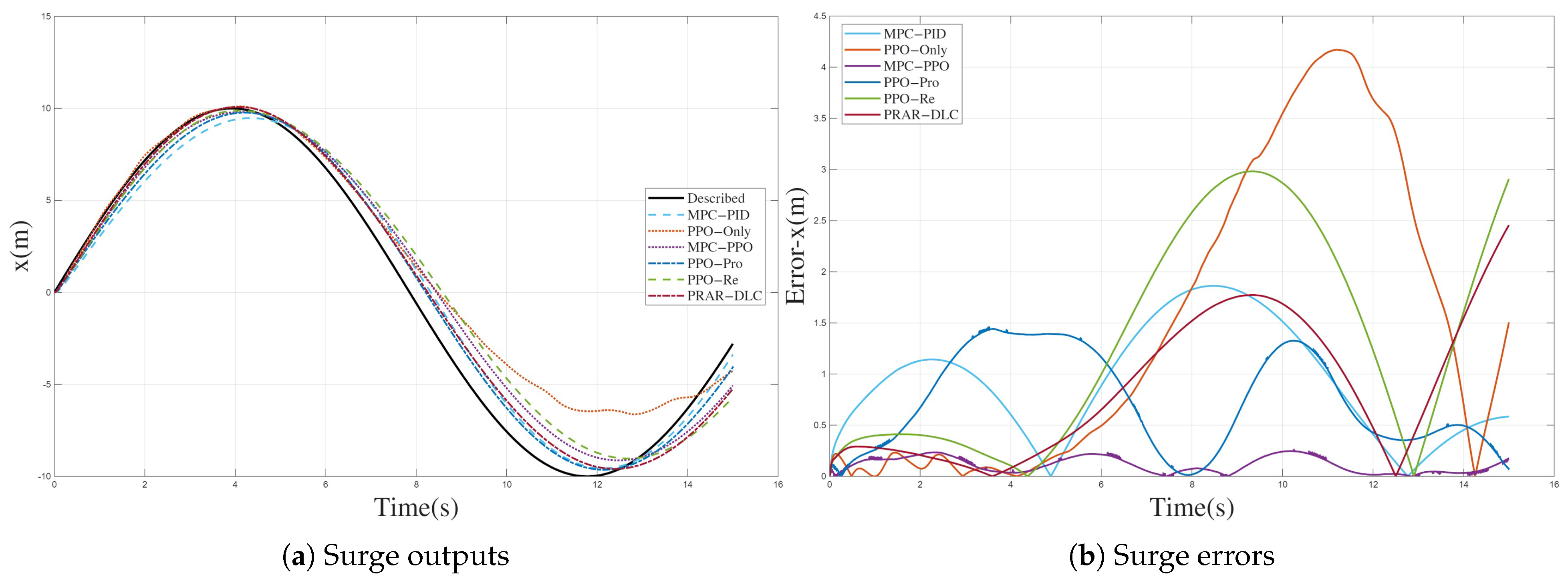
In the surge direction, PRAR–DLC provides the most robust longitudinal tracking among all methods. Compared with MPC–PID, the surge MAE is reduced from $0.269$ to $0.138$ (about $49\%$ reduction), and the RMS error decreases from $0.357$ to $0.171$ (more than $50\%$). The maximum and 95th–percentile surge errors drop from $0.963/0.843$ to $0.337/0.306$, corresponding to reductions of approximately $65\%$ and $64\%$, respectively. Although PPO–Pro and PPO–Re achieve slightly smaller MAE, their peak and tail errors remain noticeably larger than those of PRAR–DLC, and MPC–PPO suffers from much larger, near–divergent errors. The surge error curves in Figure 9b confirm that PRAR–DLC keeps the longitudinal error tightly bounded over the entire horizon, while several PPO variants accumulate substantial drift. These results indicate that the proposed proactive–reactive adaptive reward effectively suppresses large outliers and rare extreme errors in the longitudinal motion.

In the sway direction, PRAR–DLC does not minimize the average error but offers a reasonable trade–off between accuracy and robustness. Its sway MAE ($0.577$) is much smaller than those of PPO–Only and MPC–PPO (both above $1.0$). The RMS, maximum and 95th-percentile sway errors of PRAR–DLC are moderately larger than those of MPC–PID, but remain in the same order of magnitude. As shown in Figure 10b, PRAR–DLC produces a relatively smooth and bounded lateral error, whereas PPO–Only and MPC–PPO exhibit persistent bias and strong oscillations. This behavior suggests that the current PRAR design intentionally prioritises longitudinal tracking and global trajectory shape, accepting a certain increase in lateral peak error compared with the nominal-model PID, while still clearly outperforming purely learning–based controllers.

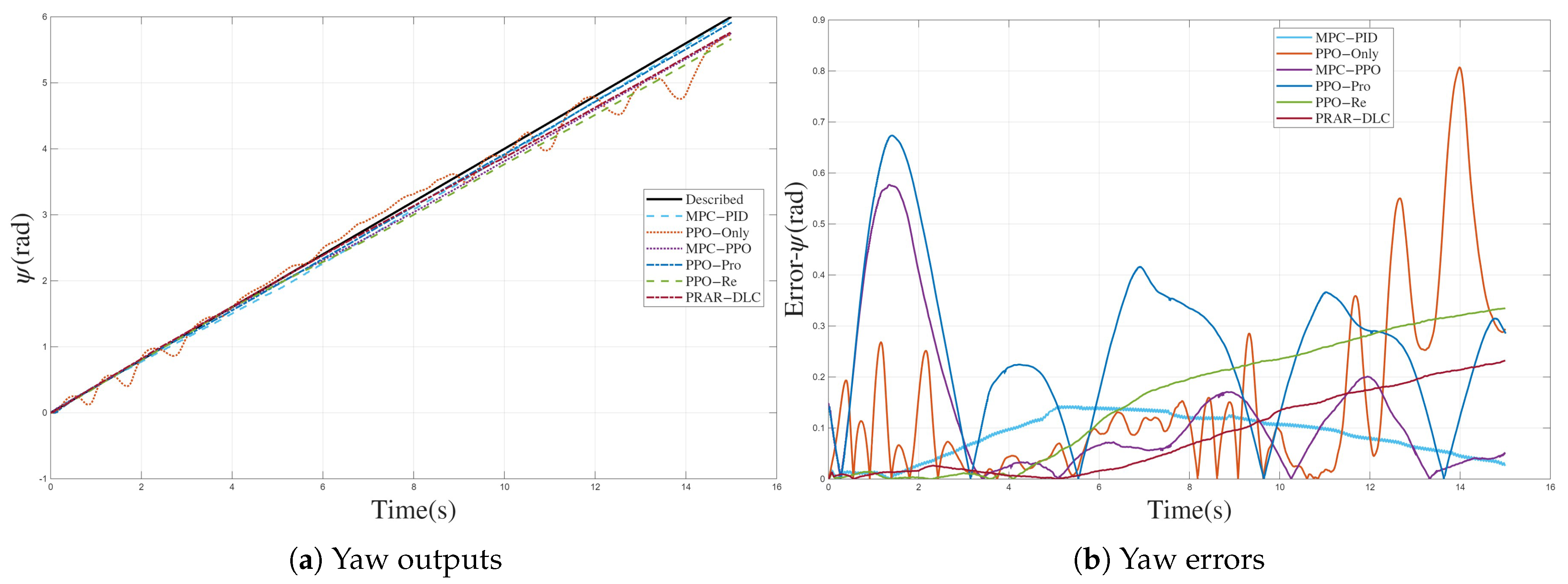
For yaw control, PRAR–DLC again exhibits competitive performance. Its yaw MAE ($0.071$) is slightly larger than that of MPC–PID ($0.060$) but clearly lower than those of PPO–Only ($0.104$) and MPC–PPO ($0.193$), and comparable to PPO–Pro ($0.073$). As shown in Figure 11b, PRAR–DLC yields a low-amplitude, low-frequency heading error without pronounced spikes, whereas the learning–only baselines produce stronger oscillations and intermittent peaks. Overall, the curvilinear trajectory experiments show that, under a weak–model assumption with an outer–loop kinematic planner and an inner PPO execution layer, PRAR–DLC can substantially reduce longitudinal errors and maintain acceptable sway and yaw performance, achieving a favorable balance between tracking accuracy and robustness compared with both the nominal–model MPC–PID controller and the RL–based baselines.

4.4. Real–Time Execution Characteristics and Physical Deployment Considerations

The runtime performance of the proposed hierarchical architecture was systematically profiled under two scenarios. In both cases, the outer $f_{\mathrm{MPC}}$ loop operates with a sampling period of $T_{\mathrm{MPC}}=0.03\mathrm{s}$ (approximately $33\mathrm{Hz}$), whereas the inner $f_{\mathrm{PPO}}$ loop runs at $T_{\mathrm{PPO}}=0.01\mathrm{s}$ (approximately $100\mathrm{Hz}$), which reflects the intended hierarchical design where the PPO-based thrust allocation reacts faster than the MPC–based kinematic planning. For each scenario, we recorded the average and maximum solution times of the MPC quadratic program, as well as the average and maximum forward–pass times of the PPO policy network. To emulate adverse operating conditions and assess robustness against fast perturbations, a bounded high-frequency disturbance at $50\mathrm{Hz}$ is injected into the surge force and yaw moment channels. This frequency is chosen to be close to the Nyquist limit of the inner–loop sampling period $T_{\mathrm{PPO}}=0.01\mathrm{s}$, so that, after discretization, it appears as a rapidly alternating excitation at each PPO control step. The disturbance amplitude is selected to remain well below the maximum thrust and torque capabilities of the water–jet actuators, ensuring physical plausibility while still providing a stringent high–frequency stress test for both the inner–loop PPO controller and the outer–loop MPC layer [35].

4.4.1. Runtime Performance in Circular Trajectory Tracking Experiments

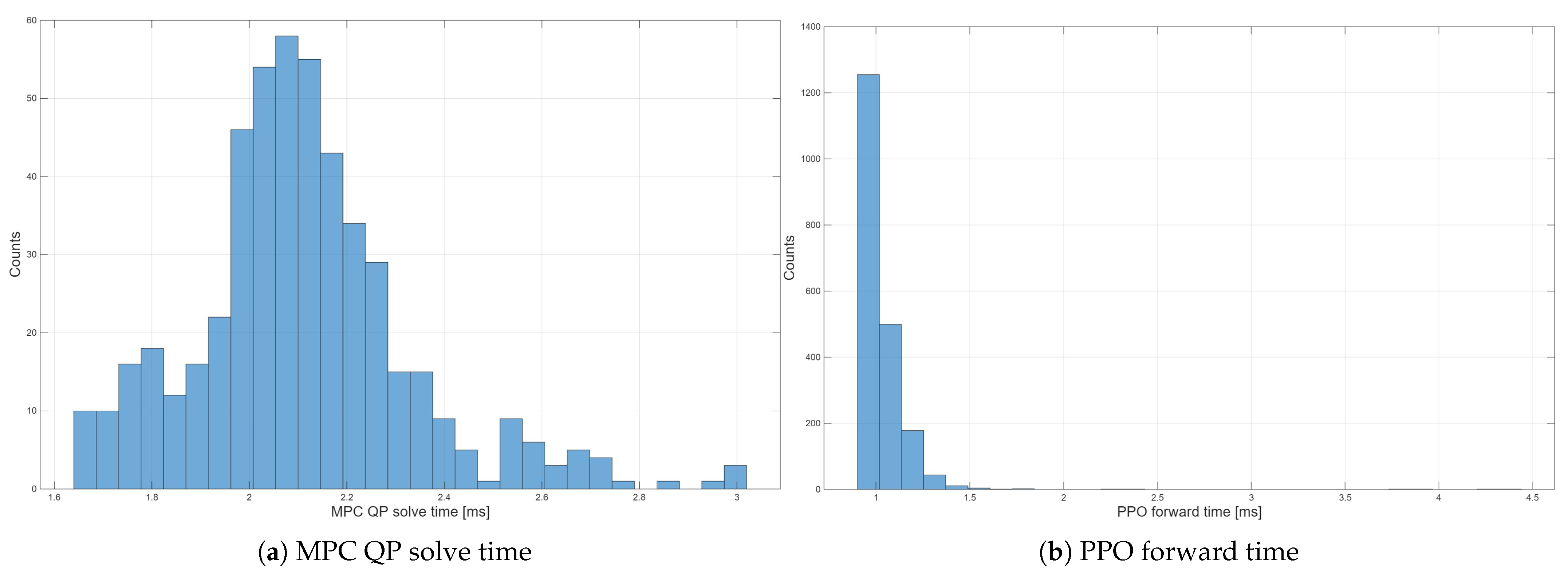
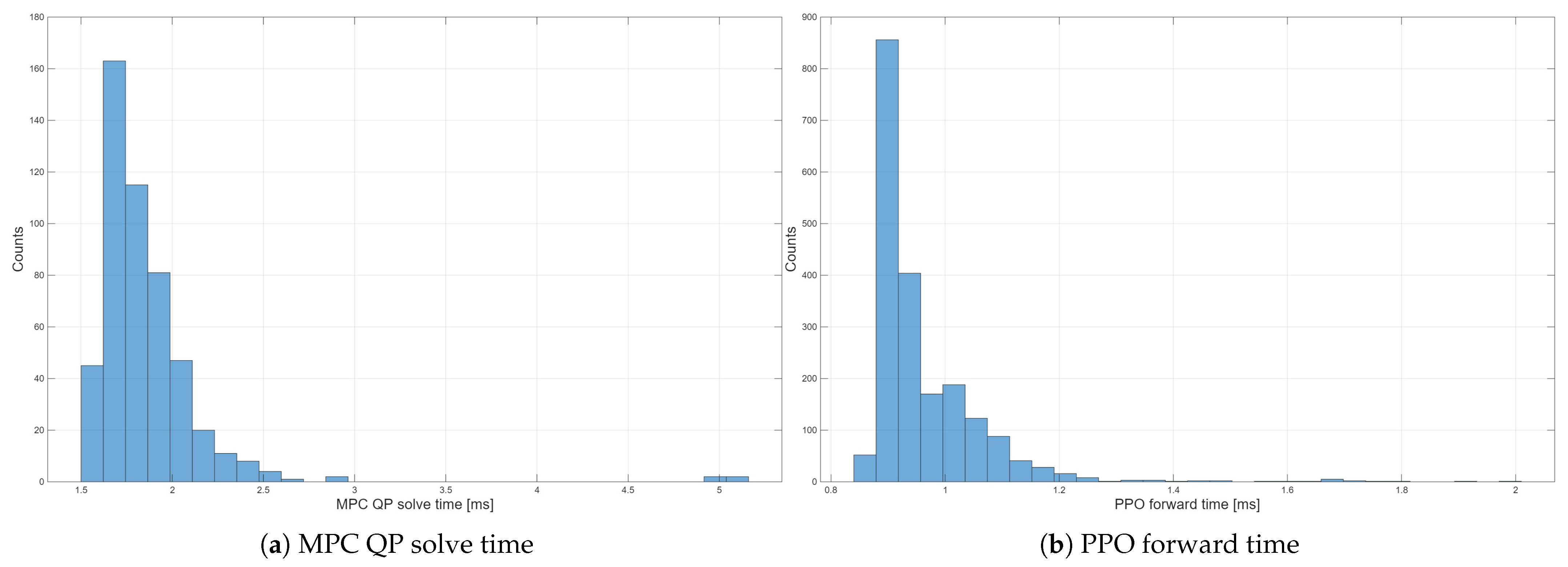
The real–time execution performance of the MPC–PPO and PRAR–DLC controllers in the circular trajectory tracking experiments is illustrated in Figure 12 and Figure 13 and summarized in and

Table 7. Runtime statistics of circular trajectory tracking experiments.

Method	Mean MPC Solve Time (ms)	Max MPC Solve Time (ms)	Mean PPO Forward Time (ms)	Max PPO Forward Time (ms)
MPC–PPO	2.108	3.010	1.030	4.439
PRAR–DLC	1.862	5.158	0.962	2.007

.

As shown in Figure 12 and Figure 13 and Table 7, the proposed hierarchical architecture is compatible with real-time implementation. Under the MPC–PPO baseline, the mean and maximum MPC QP solve times are $2.108\mathrm{ms}$ and $3.010\mathrm{ms}$, while the mean and maximum PPO forward times are $1.030\mathrm{ms}$ and $4.439\mathrm{ms}$. With the PRAR–DLC controller, the average MPC load is further reduced to $1.862\mathrm{ms}$, and the PPO forward time remains below $1\mathrm{ms}$ on average, with a maximum of $2.007\mathrm{ms}$. Comparing these figures with the sampling periods of the two loops, $T_{\mathrm{MPC}}=0.03\mathrm{s}$ ($f_{\mathrm{MPC}}\approx 33.3\mathrm{Hz}$) and $T_{\mathrm{PPO}}=0.01\mathrm{s}$ ($f_{\mathrm{PPO}}=100\mathrm{Hz}$), indicates that the average computational cost occupies less than each loop’s sampling interval.

4.4.2. Runtime Performance in Curvilinear Trajectory Tracking Experiments

The real-time execution performance of the MPC–PPO and PRAR–DLC controllers in the curvilinear trajectory tracking experiments is illustrated in Figure 14 and Figure 15 and summarized in and

Table 8. Runtime statistics of curvilinear trajectory tracking experiments.

Method	Mean MPC Solve Time (ms)	Max MPC Solve Time (ms)	Mean PPO Forward Time (ms)	Max PPO Forward Time (ms)
MPC–PPO	2.124	3.351	1.136	2.537
PRAR–DLC	1.813	6.244	0.934	1.572

.

For the curvilinear trajectory tracking experiments, the runtime behavior reported in Table 8 and Figure 14 and Figure 15 complements the circular trajectory results and illustrates how the proposed architecture behaves under more aggressive, non–uniform maneuvers. Under the MPC–PPO controller, the mean and maximum MPC QP solve times are $2.124\mathrm{ms}$ and $3.351\mathrm{ms}$, while the PPO forward pass requires $1.136\mathrm{ms}$ on average with a worst case of $2.537\mathrm{ms}$. When the PRAR–DLC scheme is activated, the computational footprint of both loops is further reduced: the average MPC time drops to $1.813\mathrm{ms}$ and the PPO forward time to $0.934\mathrm{ms}$, with a maximum of $1.572\mathrm{ms}$. These results indicate that the PRAR mechanism enables PRAR–DLC to achieve faster MPC solving and PPO inference compared with the MPC–PPO controller. Moreover, the total computation time required for each update of the hierarchical control system remains well below the system sampling period, thereby satisfying real–time execution requirements. Hence, the additional optimization burden introduced by the outer MPC does not violate real–time constraints and the two loops can be scheduled independently in practice.

From a conceptual implementation viewpoint, these timing margins imply that the hierarchical controller can be executed on a realistic onboard computing platform—sharing CPU resources with sensing, navigation and communication modules—without saturating computational capacity or degrading the closed–loop behavior of the physical USV under practical operating conditions.

Although the dual–loop controller combines MPC, PRAR and PPO and is therefore more computationally demanding than classical single–loop PID or backstepping schemes, its algorithmic complexity remains modest from the perspective of a realistic shipborne computer. In each inner–loop period, the controller solves a small-scale quadratic program with three control inputs and a fixed control horizon, performs a few vector operations over the prediction horizon for the PRAR weighting, and executes one forward pass through two fully connected neural network layers of size 512. This results in roughly ${10}^5$–${10}^6$ basic arithmetic operations per step, which is several orders of magnitude below the processing capability of typical industrial embedded CPUs or onboard PCs used on USVs. Together with the measured runtimes reported in the previous tables, this shows that the computational cost of the proposed algorithm is well matched to practical hardware resources and remains comfortably below the real–time limits.

From a physical implementation viewpoint, these generous timing and capacity margins imply that the hierarchical controller can run reliably on a realistic onboard computing platform while sharing CPU resources with sensing, navigation and communication modules. The additional computation introduced by the dual–loop structure does not saturate the processor or introduce harmful delays, and thus does not degrade the closed–loop behavior of the physical USV under practical operating conditions. On the contrary, the extra complexity is a deliberate design choice that trades inexpensive modern computation for improved constraint handling, stability and disturbance rejection. Therefore, the computational complexity of the proposed architecture is not expected to have a negative impact on a real shipborne control system; instead, it is a necessary condition for achieving high–performance trajectory tracking.

5. Conclusions

This study proposes a dual–loop USV trajectory–tracking framework that combines MPC with PPO. The USV dynamics are explicitly decoupled into a kinematic layer and a dynamic layer, for which the outer and inner controllers are designed, respectively. In the outer loop, an MPC planner operating in the inertial reference frame uses a kinematic model and explicit velocity and safety constraints to generate dynamically feasible body–fixed velocity references together with a prediction sequence over the horizon. In the inner loop, a PPO–based execution controller operating in the body–fixed reference frame learns the nonlinear inverse mapping from commanded velocities to multi-thruster forces and performs online compensation for unmodeled hydrodynamics and external disturbances. This design enforces a feasible–first–then–refine behavior, in which the policy is guided to remain within the outer–loop feasible set while progressively improving tracking accuracy. Building on this dual-loop structure, we further design a Proactive–Reactive Adaptive Reward (PRAR) mechanism that fully exploits the outer loop’s prediction sequence in combination with real–time pose–tracking errors: PRAR derives a time–weighted trajectory–complexity measure from the predicted velocities and adaptively reweights the surge, sway and yaw components of the reward, allowing the controller to anticipate upcoming aggressive maneuvers while remaining sensitive to instantaneous deviations.

The simulation results on both circular and curvilinear trajectories show that the USV controlled by the proposed framework maintains high–precision tracking under disturbances and model mismatch. Compared with a nominal hydrodynamic MPC–PID baseline, the PRAR–driven dual–loop controller reduces surge MAE and maximum longitudinal error on the curvilinear trajectory from 0.269 m and 0.963 m to 0.138 m and 0.337 m, respectively, and achieves about an 8.5% reduction in surge MAE on the circular trajectory while keeping sway and yaw MAE at a level comparable to the baseline. Across all scenarios, it also significantly suppresses error tails and avoids the large drifts or oscillations observed in PPO–Only, MPC–PPO and other PPO variants, confirming strong robustness. In addition, the proposed PRAR mechanism integrates the outer–loop MPC prediction sequence with real–time pose errors to adaptively reweight the reward, which, compared with fixed–weight PPO, improves generalization capability while keeping the average MPC and PPO computation times in the low–millisecond range, compatible with real–time on–board implementation.

Future work will focus on two directions. First, hardware–in–the–loop and full-scale waterborne experiments will be conducted to validate the controller under unmodeled actuator dynamics, onboard sensor noise, and network–induced latency. Second, to further reduce computation load and facilitate deployment on resource–limited USVs, we will investigate model lightweighting, including reduced–order MPC, neural surrogate models for prediction, and compact policy networks for thrust allocation. Extending the framework to over–actuated USVs and cooperative multi–vessel missions also constitutes a promising direction for the hierarchical architecture introduced in this study.

References

1. Gonzalez-Garcia, A.; Castañeda, H. Guidance and control based on adaptive sliding mode strategy for a USV subject to uncertainties. IEEE J. Ocean. Eng. 2021, 46, 1144–1154. [Google Scholar] [CrossRef]
2. Er, M.J.; Ma, C.; Liu, T.; Gong, H. Intelligent motion control of unmanned surface vehicles: A critical review. Ocean. Eng. 2023, 280, 114562. [Google Scholar]
3. Xu, W.; Zhang, X.; Miao, Z. Cooperative trajectory tracking control of USV-UAV with non-singular sliding mode surface and RBF neural network. Ocean. Eng. 2025, 337, 121872. [Google Scholar] [CrossRef]
4. Wei, J.; Zhang, J.; Dong, H.; Liu, Z. Prescribed-time trajectory tracking control for underactuated usv with input amplitude and rate constraints. Ocean. Eng. 2025, 326, 120891. [Google Scholar] [CrossRef]
5. Zhu, Y.; Li, Z.; Li, Y.; Yuan, C.; Guo, G. Multi-target tracking and surrounding control for multi-USV system under unknown disturbances based on distributed nmpc. Ocean. Eng. 2025, 338, 121972. [Google Scholar] [CrossRef]
6. Xu, X.; Zhang, X.; Zhang, Z.; Ma, F.; Guan, C.; Steyskal, F. Los guidance for fuzzy adaptive fault-tolerant path following control of USV with side-slip compensation and actuator fault. IEEE Trans. Transp. Electrif. 2024, 11, 6875–6886. [Google Scholar]
7. Chen, G.; Wang, W.; Dong, J. Performance-optimize adaptive robust tracking control for USV-UAV heterogeneous systems with uncertainty. IEEE Trans. Veh. Technol. 2025, 74, 7251–7262. [Google Scholar] [CrossRef]
8. Zhang, H.; Zhao, Z.; Wei, Y.; Liu, Y.; Wu, W. A self-tuning variable universe fuzzy pid control framework with hybrid bas-pso-sa optimization for unmanned surface vehicles. J. Mar. Sci. Eng. 2025, 13, 558. [Google Scholar] [CrossRef]
9. Cao, X.; Zheng, Y.; Xiao, H.; Xiao, M. Multi-target point path planning and tracking of unmanned surface vehicle using sflos algorithm and incremental pid control with crane-assisted. IEEE Access 2025, 13, 44620–44635. [Google Scholar] [CrossRef]
10. Fossen, T.I.; Pettersen, K.Y.; Galeazzi, R. Line-of-sight path following for dubins paths with adaptive sideslip compensation of drift forces. IEEE Trans. Control Syst. Technol. 2014, 23, 820–827. [Google Scholar]
11. Chen, G.; Huang, Z.; Wang, W.; Yang, S. A novel dynamically adjusted entropy algorithm for collision avoidance in autonomous ships based on deep reinforcement learning. J. Mar. Sci. Eng. 2024, 12, 1562. [Google Scholar] [CrossRef]
12. Wang, Y.-L.; Wang, C.-C.; Han, Q.-L.; Wang, X. Networked and deep reinforcement learning-based control for autonomous marine vehicles: A survey. IEEE Trans. Syst. Man Cybern. Syst. 2024, 55, 4–17. [Google Scholar] [CrossRef]
13. Xiong, Y.; Wang, S.; Tian, H.; Liu, G.; Shan, Z.; Yin, Y.; Tao, J.; Ye, H.; Tang, Y. Spatiotemporal meta-reinforcement learning for multi-USV adversarial games using a hybrid gat-transformer. J. Mar. Sci. Eng. 2025, 13, 1593. [Google Scholar] [CrossRef]
14. Rao, J.; Wang, C.; Liu, M.; Chen, J.; Lei, J.; Giernacki, W. A deep reinforcement learning approach and its application in multi-USV adversarial game simulation. Appl. Intell. 2025, 55, 1–24. [Google Scholar] [CrossRef]
15. Liu, Y.; Chen, C.; Qu, D.; Zhong, Y.; Pu, H.; Luo, J.; Peng, Y.; Xie, J.; Zhou, R. Multi-usv system antidisturbance cooperative searching based on the reinforcement learning method. IEEE J. Ocean. Eng. 2023, 48, 1019–1047. [Google Scholar] [CrossRef]
16. Cui, Z.; Guan, W.; Zhang, X. USV formation navigation decision-making through hybrid deep reinforcement learning using self-attention mechanism. Expert Syst. Appl. 2024, 256, 124906. [Google Scholar]
17. Zhou, Y.; Gong, C.; Chen, K. Adaptive control scheme for USV trajectory-tracking under complex environmental disturbances via deep reinforcement learning. IEEE Internet Things J. 2025, 11, 15181–15196. [Google Scholar] [CrossRef]
18. Wu, C.; Yu, W.; Liao, W.; Ou, Y. Deep reinforcement learning with intrinsic curiosity module based trajectory tracking control for usv. Ocean. Eng. 2024, 308, 118342. [Google Scholar] [CrossRef]
19. Wen, Y.; Chen, Y.; Guo, X. Usv trajectory tracking control based on receding horizon reinforcement learning. Sensors 2024, 24, 2771. [Google Scholar] [CrossRef]
20. Wang, Y.; Cao, J.; Sun, J.; Zou, X.; Sun, C. Path following control for unmanned surface vehicles: A reinforcement learning-based method with experimental validation. IEEE Trans. Neural Netw. Learn. Syst. 2023, 35, 18237–18250. [Google Scholar]
21. Dai, S.-L.; He, S.; Wang, M.; Yuan, C. Adaptive neural control of underactuated surface vessels with prescribed performance guarantees. IEEE Trans. Neural Netw. Learn. Syst. 2018, 30, 3686–3698. [Google Scholar]
22. Huang, W.; Cui, Y.; Li, H.; Wu, X. Effective probabilistic neural networks model for model-based reinforcement learning USV. IEEE Trans. Autom. Sci. Eng. 2025, 22, 11625–11641. [Google Scholar] [CrossRef]
23. Cui, Y.; Shi, W.; Yang, H.; Shao, C.; Peng, L.; Li, H. Probabilistic model-based reinforcement learning unmanned surface vehicles using local update sparse spectrum approximation. IEEE Trans. Ind. Inform. 2023, 20, 1283–1293. [Google Scholar]
24. Qin, H.; Tan, P.; Chen, Z.; Sun, M.; Sun, Q. Deep reinforcement learning based active disturbance rejection control for ship course control. Neurocomputing 2022, 484, 99–108. [Google Scholar]
25. Zhu, K.; Zhang, G.; Zhu, C.; Niu, Y.; Liu, J. A bi-level optimization strategy for flexible and economic operation of the chp units based on reinforcement learning and multi-objective mpc. Appl. Energy 2025, 391, 125850. [Google Scholar]
26. Liao, Y.; Yu, G.; Chen, P.; Zhou, B.; Li, H. Integration of decision-making and motion planning for autonomous driving based on double-layer reinforcement learning framework. IEEE Trans. Veh. Technol. 2023, 73, 3142–3158. [Google Scholar]
27. Hu, L.; Ding, L.; Yang, H.; Liu, T.; Zhang, A.; Chen, S.; Gao, H.; Xu, P.; Deng, Z. Lno-driven deep rl-mpc: Hierarchical adaptive control architecture for dynamic legged locomotion. IEEE Trans. Ind. Inform. 2025, 21, 8574–8584. [Google Scholar]
28. Fossen, T.I. Handbook of Marine Craft Hydrodynamics and Motion Control; John Wiley & Sons: Hoboken, NJ, USA, 2011. [Google Scholar]
29. Gonzalez-Garcia, A.; Barragan-Alcantar, D.; Collado-Gonzalez, I.; Garrido, L. Adaptive dynamic programming and deep reinforcement learning for the control of an unmanned surface vehicle: Experimental results. Control. Eng. Pract. 2021, 111, 104807. [Google Scholar] [CrossRef]
30. Li, W.; Zhang, X. Data-driven model predictive control for underactuated USV path tracking with unknown dynamics. Ocean. Eng. 2025, 333, 121457. [Google Scholar] [CrossRef]
31. Jin, L.; Liu, L.; Wang, X.; Shang, M.; Wang, F.-Y. Physical-informed neural network for mpc-based trajectory tracking of vehicles with noise considered. IEEE Trans. Intell. Veh. 2024, 9, 4493–4503. [Google Scholar] [CrossRef]
32. Schulman, J.; Wolski, F.; Dhariwal, P.; Radford, A.; Klimov, O. Proximal policy optimization algorithms. arXiv 2017, arXiv:1707.06347. [Google Scholar] [CrossRef]
33. Yan, Q.; Wu, X.; Wang, J.; Fortino, G.; Pupo, F.; Yin, M. Egcarl: A ppo-based reinforcement learning method with expert guidance and dynamic rewards for autonomous driving. Inf. Fusion 2025, 126, 103606. [Google Scholar] [CrossRef]
34. Ramezani, M.; Alandihallaj, M.A.; Yalçın, B.C.; Mendez, M.A.O.; Hein, A.M. Fuel-aware autonomous docking using rl-augmented mpc rewards for on-orbit refueling. Acta Astronaut. 2025, 238, 690–705. [Google Scholar] [CrossRef]
35. Wang, X.; Yi, H.; Xu, J.; Xu, C.; Song, L. Pid controller based on improved ddpg for trajectory tracking control of USV. J. Mar. Sci. Eng. 2024, 12, 1771. [Google Scholar] [CrossRef]
Figure 1. Inertial and body–fixed reference frames.
Jmse 13 02392 g001
Figure 2. Overall control architecture.
Jmse 13 02392 g002
Figure 3. Mechanism of PRAR.
Jmse 13 02392 g003
Figure 4. Trajectory tracking results.
Jmse 13 02392 g004
Figure 5. Surge outputs and errors.
Jmse 13 02392 g005
Figure 6. Sway outputs and errors.
Jmse 13 02392 g006
Figure 7. Yaw outputs and errors.
Jmse 13 02392 g007
Figure 8. Trajectory tracking results.
Jmse 13 02392 g008
Figure 9. Surge outputs and errors.
Jmse 13 02392 g009
Figure 10. Sway outputs and errors.
Jmse 13 02392 g010
Figure 11. Yaw outputs and errors.
Jmse 13 02392 g011
Figure 12. MPC–PPO solve time.
Jmse 13 02392 g012
Figure 13. PRAR–DLC solve time.
Jmse 13 02392 g013
Figure 14. MPC–PPO solve time.
Jmse 13 02392 g014
Figure 15. PRAR–DLC solve time.
Jmse 13 02392 g015