A Hybrid Statistical and Neural Network Method for Detecting Abnormal Ship Behavior Using Leisure Boat Sea Trial Data in a Marina Port

Abstract

Effective abnormal behavior detection in ship operations is essential for ensuring navigational safety and operational efficiency in marina ports. This study presents a hybrid method that integrates statistical analysis and neural network modeling to detect abnormal behavior based on data obtained through leisure boat sea trials. Detection criteria were established based on ship motion characteristics, operating area conditions, and the properties of the sea trial data. The method combines Rayda’s criterion and standard deviation thresholds to identify sudden changes in measured data, while a Long Short-Term Memory (LSTM) network is used to predict normal ship behavior. Deviations between predicted and measured values were evaluated using three thresholds (levels 1, 2, and 3), with level 3 effectively isolating the most significant abnormal data (representing 2–10% of the data). The proposed method is capable of successfully identifying sudden acceleration or deceleration, unusual course changes, extended stationary periods, deviations from expected routes, complex maneuvers, and track continuity issues. The results demonstrate that the proposed hybrid method can reliably distinguish abnormal ship behaviors based on real sea trial data. To separate true abnormalities from false alarms or sensor and environmental noise, its practical application on a real ship is planned as future work. This study provides a foundation for intelligent ship monitoring systems and supports the development of autonomous and semi-autonomous navigation technologies.

1. Introduction

Maritime safety is one of the primary concerns in port environments, which are characterized by increased traffic density and complex ship operations. In particular, marina areas are known for frequent minor accidents and collisions, although often not officially documented. Common causes include operator error due to inadequate situational awareness, delayed responses to unexpected ship motions, adverse weather conditions, or mechanical failures. In addition, Kim et al. [1] noted that the confined space within marina ports often leads to ship entanglement and unintended contact between ships. Such factors directly influence ship behaviors and can escalate into hazardous situations. Therefore, the real-time identification of abnormal ship behavior is essential to enable operators to respond promptly to early warnings. Wang et al. [2] defined abnormal ship behaviors as behavioral patterns that are markedly different from normal behavior, based on changes in ship motion states. However, if the ship motion states collected from sensors are influenced by system or environmental disturbances, these effects may contaminate the data. As a result, such disturbances could be incorrectly categorized as abnormal ship behaviors. This variability makes it difficult to define universal standards for detecting abnormal motion behavior (Ksciuk et al. [3]; Baig et al. [4]). Leisure boats exhibit dynamic characteristics that differ significantly from those of commercial ships. This difference arises from their smaller size, lighter displacement, and higher sensitivity to environmental disturbances such as wind and waves. In addition, their maneuvering data are highly nonlinear and often affected by human steering inputs, which makes conventional models less effective. Therefore, developing a dedicated modeling approach is necessary to accurately represent the dynamic behavior of leisure boats.

Various previous studies have proposed criteria to detect abnormal commercial ship behaviors, most commonly using Automatic Identification System data. Some approaches rely on trajectory-based methods, such as Rayda’s criterion (Nie et al. [5]; Shi et al. [6]), while others use statistical tools, such as the standard deviation, to identify abnormal variations in speed or heading (Zhang et al. [7]; Rong et al. [8]). Other studies have incorporated environmental and traffic data to minimize false alarms (Radon et al. [9]). However, these methods often depend heavily on expert-defined thresholds and may not adapt well to changing operating conditions (Yan and Wang [10]; Iphar et al. [11]). Recent studies have introduced machine learning-based approaches for automated behavior detection. These included feature-based and clustering models (Rong et al. [12]; Ma et al. [13]), as well as unsupervised learning methods such as autoencoders and deep neural networks (Sadeghi and Matwin [14]). While effective, many of these models have difficulty capturing the temporal dependencies of ship motion or the influence of environmental factors and nearby vessels. The Long Short-Term Memory (LSTM) network has proven particularly effective for maritime applications as its memory cells can store temporal information, enabling accurate modeling of ship trajectories and dynamic behaviors. LSTM-based models have been used for route prediction and abnormal behavior detection, often enhanced with clustering algorithms, attention mechanisms, or hybrid deterministic probabilistic designs to improve their prediction accuracy (Li et al. [15]; Lee and Yang [16]; Liu et al. [17]; Guo et al. [18]; Wang and Fu [19]; Sun et al. [20]; Zaman et al. [21]; Yang et al. [22]).

Unlike previous studies, which have mainly relied on AIS data of commercial ships and applied statistical or machine learning-based anomaly detection methods separately. This study targets leisure boats operating in marina ports, where their behavior is more variable and less predictable (Wolsing et al. [23]; Ying et al. [24]). Leisure boats are often operated by non-professional users, increasing the risk of erratic maneuvers and operational uncertainty (Tyasayumranani et al. [25]). To address this challenge, this study proposes a hybrid abnormal behavior detection method that integrates statistical techniques (Rayda’s criterion and standard deviation) with an LSTM-based predictive model trained on sea trial data. This framework enables the identification of abnormal patterns such as sudden acceleration or deceleration, unusual course changes, extended stationary periods, deviations from expected routes, complex maneuvers, and track continuity issues (Zhang et al. [26]; Li et al. [27]). This improvement advances existing methods by combining the interpretive clarity of statistical criteria with the temporal learning capability of neural networks. As a result, it enhances safety evaluation, system testing, and operational monitoring in congested port environments. However, this study focuses solely on general abnormal behavior detection. It does not distinguish between true anomalies and false alarms caused by sensor noise or environmental disturbances.

The remainder of this paper is organized as follows: Section 2 describes the criteria established for the abnormal ship behavior detection based on leisure boat sea trial data. Section 3 introduces the proposed hybrid abnormal behavior detection framework and presents the algorithms. Section 4 presents the LSTM model training results, the predicted normal behavior, and the analysis of the detected abnormal behaviors. Finally, Section 5 concludes the study and discusses potential directions for future work, including real-ship applications and system improvements.

2. Establishment of Criteria for Detecting Abnormal Ship Behavior

2.1. Target Ship and Sea Trial Data

The target ship in this study is a leisure boat from AVIKUS NeuBoat, Seoul, Republic of Korea, shown in Figure 1, which was used to analyze abnormal behaviors during port operations. The boat has an overall length of 9.45 m and a displacement weight of 5275 kg. With a relatively shallow draft of 0.939 m and a trim angle of 3° at the stern, it is designed for high maneuverability in limited water spaces, making it suitable for behavioral monitoring research in port areas.

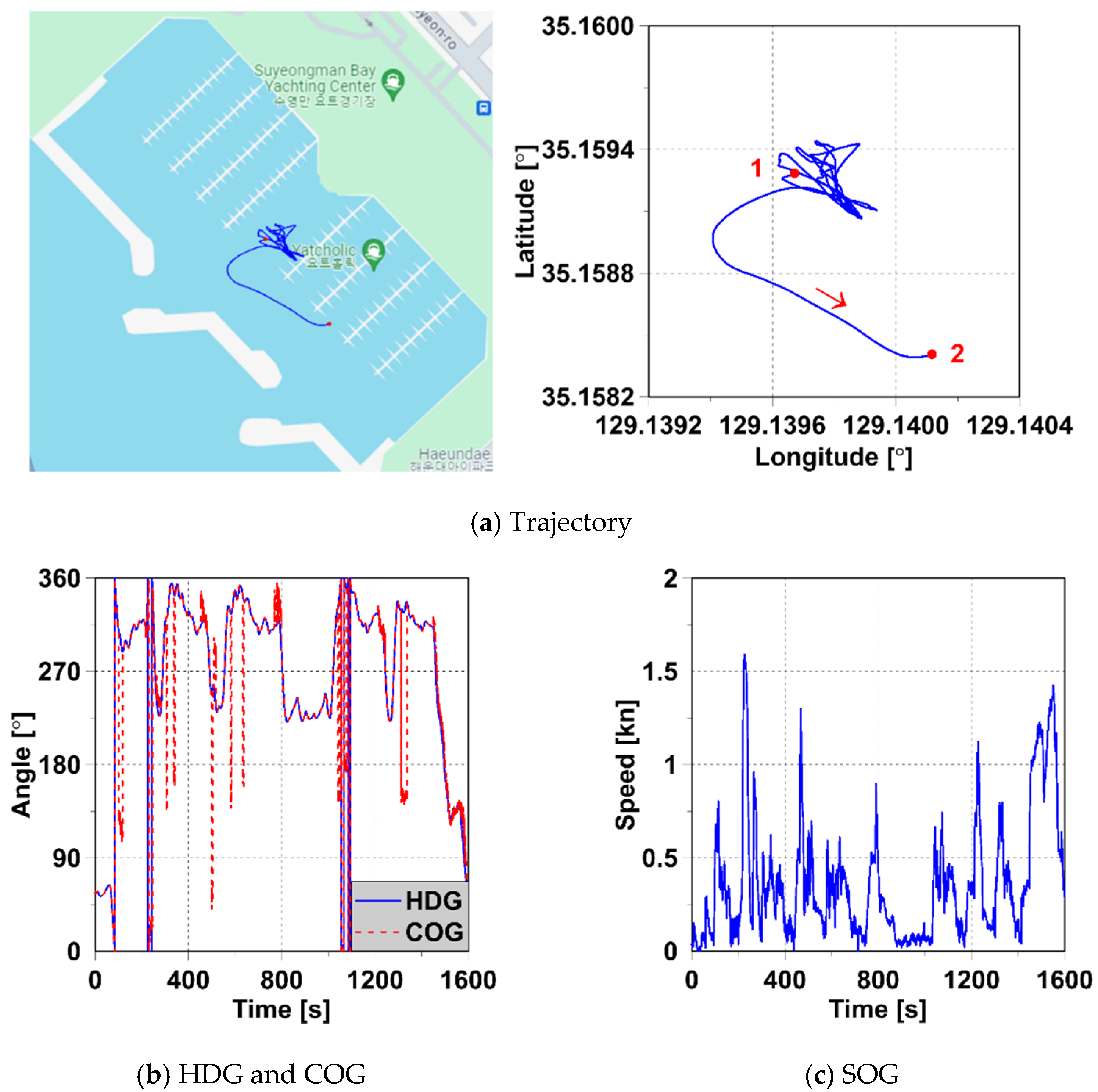
The target boat operated in Busan Marina, Busan, Republic of Korea, which is a coastal port characterized by narrow channels, high boat density, and limited maneuvering space. These features make it well-suited for testing ship behaviors in constrained environments. The boat was equipped with GPS and heading sensors that recorded its motion and trajectory data during real sea trials. The data were collected for approximately 1600 s at a sampling frequency of 10 Hz (i.e., 0.1 s intervals). The measured variables included latitude, longitude, heading (HDG), course over ground (COG), speed over ground (SOG), and rate of turn (ROT). Figure 2 shows the data collected during the entire trial. Figure 2a shows the boat’s actual path using latitude and longitude. The recording started at point 1, where the boat was stationary, and drifting slightly due to wind or current. It then moved forward, backward, and turned several times in a small area to prepare for the test. The main test involved moving the boat toward point 2. Figure 2b shows the HDG and COG values, both measured to true north. The difference between HDG and COG from 200 s to 700 s suggests possible unusual turning behavior during the preparation phase. Figure 2c shows the SOG, which remained under 1.6 kn. The speed changed often, showing that the boat accelerated, slowed down, and maintained low speeds at different times.

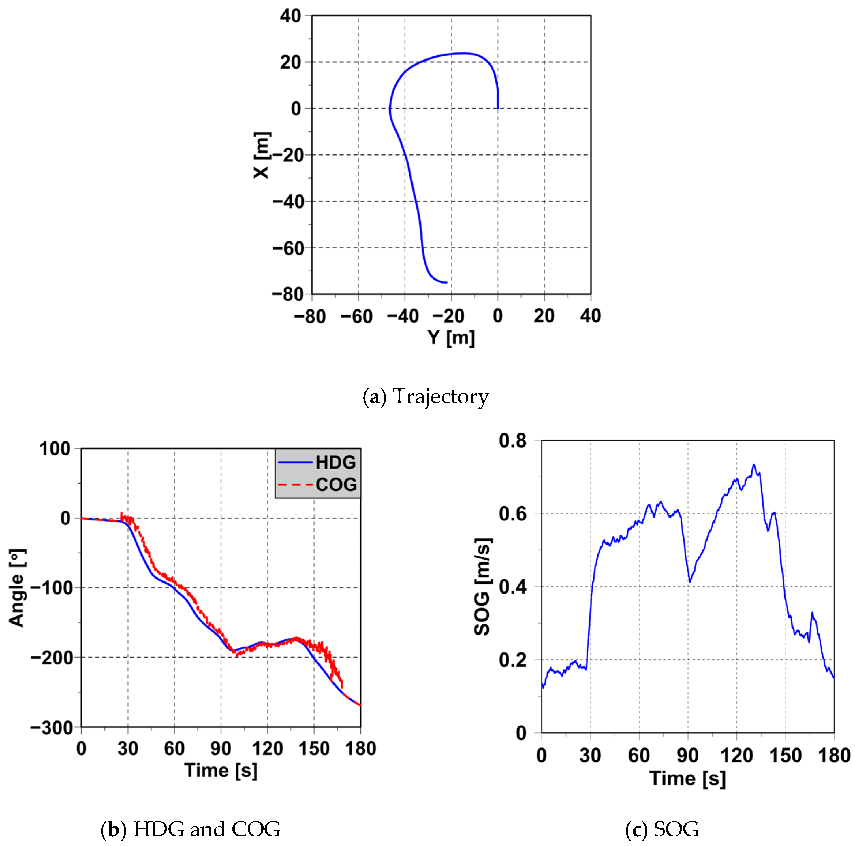
Before training the model, the raw measurements were synchronized and converted from the geographic coordinate system to the ship’s maneuvering coordinate system. Figure 3 shows the sea trial data after preprocessing. In this study, only the final 180 s of the 1600 s dataset were used for analysis. This segment represents the actual sea trial phase, while the earlier 1420 s corresponded to pre-trial preparation maneuvers and were therefore excluded. The Equidistant Cylindrical Projection (ECP) was used to convert the original trajectory shown in Figure 2a, recorded in geographic coordinates (latitude and longitude), to local metric coordinates ($X$,$Y$) (Yang [28]). This method is useful for small areas like coastal ports. The conversion uses a reference point at the start of the data (${\varphi }_0$,${\lambda }_0$), and the formulas are:

$$\begin{gathered} X_{ECP}=R\left(\lambda -{\lambda }_0\right)\mathit{cos}{\varphi }_0 \\ {Y}_{ECP}=R\left(\varphi -{\varphi }_0\right) \end{gathered}$$

(1)

where $\varphi$ and $\lambda$ are the latitude and longitude (in radians) of the data point, ${\varphi }_0$ and ${\lambda }_0$ are the latitude and longitude (in radians) of the reference point, $R$ is the Earth’s radius (assumed as 6,371,000 m), and $X$ and $Y$ are the eastward and northward distances (in meters), respectively. After conversion, the coordinate system was rotated such that the X-axis matched the boat’s initial heading (${HDG}_0$) at the start of the 180 s segment. This rotation transformed the trajectory according to the coordinate system in the ship’s maneuvering, thus making it easier to understand its maneuvering behavior. The rotation is performed as follows:

$$\left[\begin{array}{c}X\\ Y\end{array}\right]=\left[\begin{array}{cc}\mathit{cos}{\psi }_0& \mathit{sin}{\psi }_0\\ -\mathit{sin}{\psi }_0& \mathit{cos}{\psi }_0\end{array}\right]\left[\begin{array}{c}{X}_{ECP}\\ Y_{ECP}\end{array}\right]$$

(2)

where ${\psi }_0$ is the initial heading angle in radians, and $X$, $Y$ are the final rotated coordinates used in Figure 3a. In Figure 3b, both HDG and COG were converted from true north to the coordinate system in the ship’s maneuvering, where 0° points forward and the angle increases as the ship turns to starboard. In Figure 3c, SOG was converted from knots (kn) to meters per second (m/s) for consistent units.

A labeling procedure was applied to classify each data point as either normal (predicted using the LSTM model) or abnormal (identified from the actual sea trial data). Labeling was conducted based on predefined statistical rules derived from Rayda’s criterion, which quantifies deviations in motion characteristics. The specific definitions of abnormal events are described in Section 2.2.

2.2. Establishment of Criteria

Wang et al. [2] listed 16 criteria for detecting abnormal commercial ship behaviors. These criteria are organized into two primary groups—Motion and Location—which are further divided into subcategories: Speed, Track, comparison with Historical Routes, comparison with Maps, and Other situational behaviors, depending on the context. There are currently no widely accepted criteria or threshold values to define abnormal behaviors for leisure boats, as they depend heavily on the vessel’s size, hull design, speed, maneuverability, and operating conditions. For this study, criteria were established based on the motion characteristics of a leisure boat from sea trial data in a limited port. Six criteria were ultimately established, based on the following considerations:

• Sudden speed changes: Boats in port areas usually change their speed slowly. This is because ports are narrow and crowded, and there are safety rules to follow. A sudden increase or decrease in speed may indicate evasive action, mechanical issues, or unintentional throttle control, which could lead to collisions or loss of control.
• Unusual course changes: In a port, boats usually follow a smooth and steady course along marked paths. Large or sudden changes in course could mean that the boat is trying to avoid an object, has made a wrong turn, or the operator is inexperienced. These issues are more common for leisure boats, where drivers may not have formal training.
• Extended stationary periods: In a port area, boats are expected to stop only at designated docks or anchoring zones. If a leisure boat stays still for a long time outside these zones, it may indicate loitering, unauthorized activity, or engine trouble. Because space in ports is limited and tightly managed, unexpected stops can disrupt operations and raise safety or security concerns.
• Deviation from the expected route: Boats in port usually follow fixed or expected routes. Large or repeated deviations from these routes may happen if the operator does not know the local rules, is intentionally entering off-limit areas, or is experiencing navigation problems. This is especially important for leisure boats, which may not have advanced navigation systems and often rely on visual guidance. In this study, the expected route is assumed to be the normal route, which is predicted by the LSTM model.
• Complex maneuvers: Under normal port conditions, the boat moves in smooth lines and avoids sudden or complex turns. Maneuvers like zigzaging, turning, or tight looping are rare and often happen during testing, risky behavior, or when the operator loses control. Spotting these actions is important in areas where both commercial and leisure boats operate together.
• Track continuity issues: In this study, sea trial data were collected from onboard navigation sensors, which usually provide continuous tracking. However, if there are frequent gaps or missing data, it may mean that the equipment failed or someone has turned off the system on purpose. These tracking problems make it hard to monitor behavior accurately and could signal rule violations or suspicious activity.

The six criteria mentioned above were used to detect abnormal behavior of a leisure boat in the port area. To separate normal from abnormal behavior, specific thresholds are needed for each one. These thresholds are set in the next section, based on statistical analysis of the sea trial data.

3. Methodology

3.1. Rayda’s Criterion and Standard Deviation

This study used Rayda’s criterion to detect abnormal ship behaviors based on statistical deviation from normal patterns, as proposed by Shi et al. [6]. For this purpose, we assume that normal values for trajectory, course, and speed follow a normal distribution. Most values stay near the mean ($\mathsf{\mu }$), while values far from it likely indicate abnormal behaviors. The detection steps are shown in Algorithm 1. First, the mean and standard deviation ($\mathsf{\sigma }$) are calculated during a baseline period. Then, if later data points deviate by more than $\mathrm{k}·\mathsf{\sigma }$, they are marked as abnormal. Nie et al. [5] used $k$ values greater than 3 to detect only strong outliers. While this reduces false alarms, it may miss small but important changes. In this study, three threshold levels ($k$ = 1, 2, 3) were tested to strike a better balance between sensitivity and practicality; this is especially crucial for detecting small abnormal behavior in limited port areas, where even minor changes can be important.

Algorithm 1: Rayda’s criterion for abnormal behavior detection.

Input: Time-series data $D=\left\{d_i={time}_i,X_i,Y_i,{HDG}_i,{COG}_i,{SOG}_i\right\}\left|i=\mathrm{1,2},\dots ,n\right.$ Threshold multiplier $k$ Step 1: Compute the mean ${\mu }_{\nu }$ and the standard deviation ${\sigma }_{\nu }$ for each variable $\nu \in \left\{X,Y,HDG,COG,SOG\right\}$ for each time index $i=\mathrm{1,2},\dots ,n$ do     for each variable $v\in \left\{trajectory,HDG,COG,SOG\right\}$ do         if $\left|v_i-\mu \right|>k·{\sigma }_v$  then             Add $\left(t_i,v_i\right)$ to outlier set $y$          end if     end for end for Output: Outlier set $y$

3.2. Long Short-Term Memory (LSTM) Network

To capture the time-dependent patterns of ship motion and predict normal behavior, this study uses a Long Short-Term Memory (LSTM) network. The LSTM is a type of recurrent neural network (RNN) that performs well with time-series data. Unlike traditional feedforward networks, LSTMs can learn long-term dependencies by storing historical information in memory cells. These cells include three main gates: The forget gate ($f_{\mathrm{t}}$) decides which parts of the previous memory state ($c_{\mathrm{t}-1}$) should be discarded, using a sigmoid activation function to output values between 0 and 1. The input gate ($i_{\mathrm{t}}$) and candidate memory (${\tilde{c}}_{\mathrm{t}}$) determine what new information should be added to the memory. The input gate uses a sigmoid function to control the update amount, while the candidate memory uses a tanh function to generate new content. The output gate ($o_{\mathrm{t}}$) determines which parts of the updated memory state ($c_{\mathrm{t}}$) are used to compute the next hidden state ($h_{\mathrm{t}}$) and the output ($y_{\mathrm{t}}$), using both sigmoid and tanh functions. The updated memory state ($c_{\mathrm{t}}$) and hidden state ($h_{\mathrm{t}}$) are passed to the next time step. The hidden state ($h_{\mathrm{t}}$) is also used to make predictions. This gating mechanism allows the LSTM to selectively remember or forget past information, making it especially effective for predicting time-series data such as those capturing ship motion behaviors.

In this study, an LSTM network was trained using sea trial data to learn normal ship behavior based on trajectory, HDG, COG, and SOG values. The trained model then predicts the normal behavior, and differences between the predicted and actual values are used to detect abnormal behaviors. Abnormal points were identified using thresholds based on Rayda’s criterion. To find the best model, a grid search was performed over the main hyperparameters: the number of LSTM layers ($L$), the number of units per layer ($U$), and the number of training epochs ($E$). In this study, the tested values were: $L\in \left\{\mathrm{1,2},\mathrm{3,4}\right\}$, $U\in \left\{\mathrm{16,32,48,64,96,128}\right\}$, and $E\in \left\{\mathrm{10,20,30,40}\right\}$. The input was time-series data, a window size ($T$), and the defined search space. The data were converted into overlapping sequences, where each sequence of $T$ steps was used to predict the next value at $T+1$. The best model was considered to be the one with the lowest validation Mean Squared Error (MSE), ensuring good generalization. The outputs included the optimal architecture ($L*,U*$), loss histories, and MSE values for comparison. In the 180 s segment, the first 20 s were used for training and validation, while the remaining 160 s were reserved for testing. Although the training duration was short, a sliding window approach (window size $T$) was used to generate overlapping temporal samples, greatly increasing the number of effective training instances. Following standard machine learning practice, the 20 s dataset was split into training (75%) and validation (25%) subsets. The LSTM network, with its memory cells preserving temporal dependencies, effectively learned and generalized motion patterns even from these limited data. The best LSTM model determined with Algorithm 2 was then used to predict normal ship behavior, as shown in Algorithm 3. First, the input time-series data were standardized to keep the model stable during prediction. Then, a sliding window method was used to create overlapping input sequences that maintain the time order and context. These sequences were passed into the LSTM model, which used its memory to learn from past patterns and predict the next step. The model predicted multiple variables at once: trajectory, HDG, COG, and SOG. After prediction, the values were converted back to their original scale using the stored mean and standard deviation.

Algorithm 2: Grid search for LSTM model architecture.

Input: Time series data $D=\left\{d_i=\left({time}_i,X_i,Y_i,{HDG}_i,{COG}_i,{SOG}_i\right)\left|i=\mathrm{1,2},\dots ,n\right.\right\}$ Window size $T$ Grid search space:     Number of layers $L\in \mathbb{L}=\left\{\mathrm{1,2},\mathrm{3,4}\right\}$     Units per layer $U\in \mathbb{U}=\left\{\mathrm{16,32,48,64,96,128}\right\}$     Number of training epochs $E\in \mathbb{E}=\left\{\mathrm{10,20,30,40}\right\}$     Loss function $\mathcal{L}$ (Mean Squared Error) Step 1: Sequence generation Create input-output pairs from overlapping windows:                $D_{seq}=\left\{\left(d_t,d_{t+1},\dots ,d_{t+T-1}\right)\to d_{t+T}\right\}$ Step 2: Data splitting Partition into training and validation sets:                    $D_{train},D_{val}\subset D_{seq}$ Step 3: Grid search over architectures for each architecture $\left(L,U\right)\in \mathbb{L}\times \mathbb{U}$ do    Build LSTM model ${Model}_{L,U}$ with:         Input shape $\left(T,m\right)$, where $m$ is the number of variables         $L$ stacked LSTM layers, each with $U$ units    Training using $D_{train}$ for $E$ epochs, minimizing:             ${\mathcal{L}}_{train}={\displaystyle \frac{1}{n}}{\sum }_{i=1}^n{\left({\widehat{d}}_i-d_i\right)}^2$   Evaluate validation loss ${\mathcal{L}}_{val}^{\left(L,U\right)}$   Track best architecture:             $\left(L*,U*\right)=arg{min}_{\left(L,U\right)}{\mathcal{L}}_{val}^{\left(L,U\right)}$ end for Output: Final training and validation losses ${\mathcal{L}}_{train},{\mathcal{L}}_{val}$ for all $\left(L,U\right)$ Epoch-wise training history Best architecture ($L*,U*$)

Algorithm 3: LSTM model for normal behavior prediction.

Input: Time-series data $D=\left\{d_v=\left({time}_i,X_i,Y_i,{HDG}_i,{COG}_i,{SOG}_i\right)\left|i=\mathrm{1,2},\dots ,n\right.\right\}$ Window size $T$ Step 1: Data standardization for each variable $v\in \left\{X,Y,HDG,COG,SOG\right\}$ do    Compute mean ${\mu }_v$ and standard diviation ${\sigma }_v$    Normalize:                   $z_{i,v}={\displaystyle \frac{v_i-{\mu }_v}{{\sigma }_v}}\left|i=\mathrm{1,2},\dots ,n\right.$ end for Step 2: Sequence generation (Windowing) for $t=1$ to $n-T$ do    Input sequence: $Z_t=\left[z_t,z_{t+1},\dots ,z_{t+T+1}\right]\in {\mathbb{R}}^{T\times m}$, where$m=len\left(v\right)$    Target output:       $y_t=z_{t+T}$ end for Step 3: LSTM model calculation for each input sequence $Z_t$ do    for each time step $k=1$ to $T$ do        Forget gate:       $f_k=\sigma \left(W_f·\left[h_{k-1},z_{t+k-1}\right]+b_f\right)$        Input gate:        $i_k=\sigma \left(W_i·\left[h_{k-1},z_{t+k-1}\right]+b_i\right)$        Candidate cell state:   ${\tilde{c}}_k=tanh\left(W_c·\left[h_{k-1},z_{t+k-1}\right]+b_c\right)$        Cell state update:  $c_k=f_k⨀c_{k-1}+i_k⨀{\tilde{c}}_k$        Output gate:     $o_k=\sigma \left(W_o·\left[h_{k-1},z_{t+k-1}\right]+b_o\right)$       Hidden state:     $h_k=o_k⨀tanh\left(c_k\right)$      end for     Predicted output:     ${\widehat{y}}_t=W_y·h_T+b_y$ Step 4: Prediction recovery (Inverse transform) for each predicted value ${\widehat{y}}_t=\left({\widehat{z}}_{t,X},{\widehat{z}}_{t,Y},{\widehat{z}}_{t,HDG},{\widehat{z}}_{t,COG},{\widehat{z}}_{t,SOG}\right)$ do     Recover original scale: ${\widehat{v}}_{t+T}={\widehat{z}}_{t,v}·{\sigma }_v+{\mu }_v$ end for Output: Predicted normal sequence:          $\widehat{D}=\left\{{\widehat{d}}_v=\left(t_i,{\widehat{X}}_i,{\widehat{Y}}_i,{\widehat{HDG}}_i,{\widehat{COG}}_i,{\widehat{SOG}}_i\right)\left|i=T+1,\dots ,n\right.\right\}$

4. Results and Discussion

4.1. Training of LSTM Model

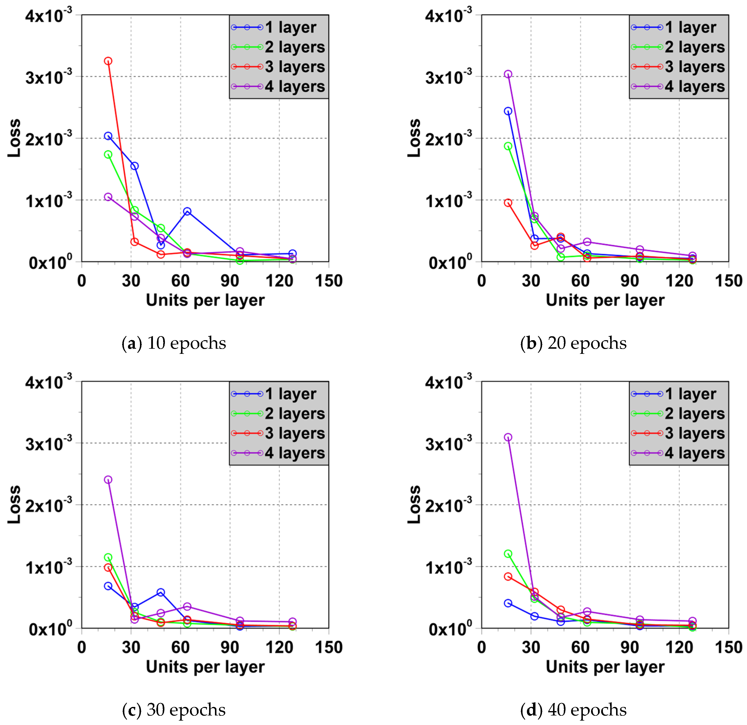
Figure 4 shows how the validation loss changed for different LSTM architectures over various training epochs. The subfigures (a to d) correspond to 10, 20, 30, and 40 epochs, respectively, and each curve shows the loss trend for models with 1 to 4 layers as the number of units increased. Figure 4a shows that the validation loss remained high, with only 10 epochs of training, especially for models with fewer hidden units. From Figure 4b, improved performance can be seen with 20 epochs, where models with more than 32 units begin to perform better and the 2- or 3-layer models consistently outperform single-layer models. Figure 4c shows that the loss values dropped more clearly for models with at least 64 units after 30 epochs, with 2-layer models showing the best balance between learning and overfitting. Finally, Figure 4d shows that 2- or 3-layer models with 96 or 128 units demonstrated the lowest losses after training for 40 epochs. In contrast, 4-layer models started to overfit and perform worse. Overall, models with 2 or 3 layers and 96 or more units performed best, especially with 30 or more epochs.

Table 1. Validation losses for different LSTM layer architectures and training epochs (units = 128).

Architecture	10 Epochs	20 Epochs	30 Epochs	40 Epochs
[128]	1.317 × 10−4	5.193 × 10−5	3.765 × 10−5	3.435 × 10−5
[128,128]	3.697 × 10−5	2.510 × 10−5	3.002 × 10−5	1.548 × 10−5
[128,128,128]	4.465 × 10−5	3.678 × 10−5	3.625 × 10−5	4.752 × 10−5
[128,128,128,128]	4.575 × 10−5	9.636 × 10−5	1.041 × 10−4	1.155 × 10−4

compares the validation losses at a fixed unit size (128) for models with different depths. The 2-layer model ([128,128]) presented the best results across all epochs, reaching the lowest loss (1.548 × 10⁻⁵) at 40 epochs. The 1-layer model improved, but remained less accurate. The 3-layer model stopped improving after 20 epochs, while the 4-layer model worsened with more training, likely due to overfitting. These results support the trend shown in Figure 4. Figure 5 shows the training and validation loss values for the best model ([128,128]) over 40 epochs. The losses dropped quickly in the first 5 epochs and then stabilized, indicating good learning and generalization ability. These results confirm that the [128,128] model trained for 40 epochs is a strong choice for predicting normal ship behavior.

4.2. Prediction of Normal Ship Behavior

After training the LSTM model with the selected architecture, it was applied to predict normal ship behavior. Figure 6 compares the predicted and actual values for trajectory, HDG, COG, and SOG, along with their Root Mean Squared Error (RMSE) values. As shown in Figure 6a, the predicted trajectory almost overlaps with the measured path, supported by a low RMSE of 0.440 m, confirming that the model accurately captures spatial motion. In Figure 6b, the HDG prediction also shows high accuracy, with an RMSE of 0.424°, indicating that the model can reproduce the ship’s heading changes with minimal error. In contrast, Figure 6c shows a relatively larger RMSE of 10.141° for COG. This higher error mainly results from noise in the measured COG, which fluctuates due to the sensitivity of the GPS-based measurements at low speeds or during turning maneuvers. The predicted COG curve was smoother, as the LSTM captures the underlying motion trend and filters out short-term disturbances. Finally, Figure 6d shows that the SOG prediction matches the measured speed almost perfectly, with an extremely low RMSE of 4.821 × 10⁻⁵ m/s, confirming the model’s ability to track speed fluctuations accurately. Overall, these quantitative results confirm that the LSTM model successfully learned the normal ship motion patterns, with only minor discrepancies in COG due to its inherently higher dynamic sensitivity.

4.3. Detection of Abnormal Ship Behaviors

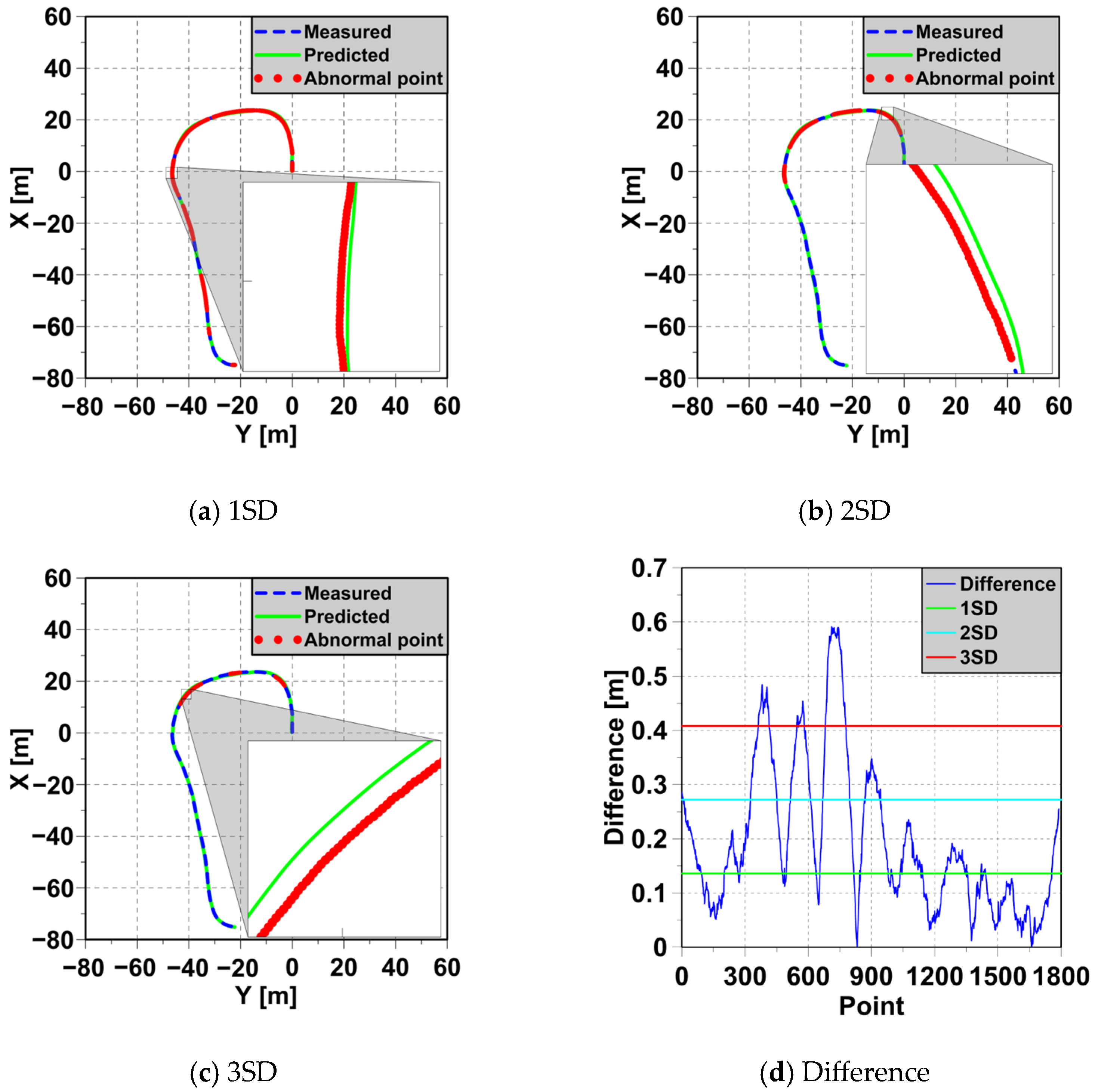
To improve the reliability of behavior monitoring in maritime operations, a two-stage anomaly detection framework was developed. In the first stage, the LSTM model was trained to learn the normal dynamic patterns of the boat from labeled sea trial data. During testing, the differences between actual and predicted values were evaluated to identify abnormal behavior. In the second stage, statistical criteria were directly applied to both the residuals and the sea trial data to quantify abnormal motion based on predefined thresholds. This hybrid integration enables the LSTM to capture nonlinear temporal dependencies in the motion sequence, while the statistical component objectively measures deviations from normal behavior. To measure the differences, standard deviation (SD)-based thresholds were applied. Three threshold levels of 1SD, 2SD, and 3SD were tested to assess the sensitivity of detecting abnormal behavior, which were identified when the difference between the actual and predicted values exceeded a given threshold. Figure 7, Figure 8, Figure 9 and Figure 10 show the results for trajectory, HDG, COG, and SOG, while

Table 2. Abnormal point statistics by threshold levels.

Threshold Value	All Points in Data	Abnormal Points	Abnormal Percentage
Trajectory
1SD = 0.136 m	1790	1056	58.994%
2SD = 0.272 m		427	23.855%
3SD = 0.408 m		183	10.223%
HDG
1SD = 0.296°	1790	605	33.799%
1SD = 0.592°		253	14.134%
3SD = 0.888°		109	6.089%
COG
1SD = 2.568°	1790	377	21.061%
2SD = 5.128°		121	6.760%
3SD = 7.692°		44	2.458%
SOG
1SD = 0.045 m/s	1790	858	47.933%
2SD = 0.090 m/s		272	15.196%
3SD = 0.135 m/s		85	4.749%

summarizes the number and percentage of detected abnormal behavior for each threshold and parameter.

For the trajectory, the detection results at the three threshold levels are presented in Figure 7. At the lowest threshold, 1SD (0.136 m), a total of 1056 abnormal points were detected out of 1790 total observations, representing 58.994%. These were spread across the route, suggesting high sensitivity. However, some normal turns may have been incorrectly flagged. At 2SD (0.272 m), 427 points (23.855%) were detected, showing reduced sensitivity. At the highest threshold of 3SD (0.408 m), only significant abnormal points were detected, with 183 points (10.223%) identified, mostly during sharp turns. Figure 7d shows that most deviations remained below the 2SD line, with a few exceeding 3SD.

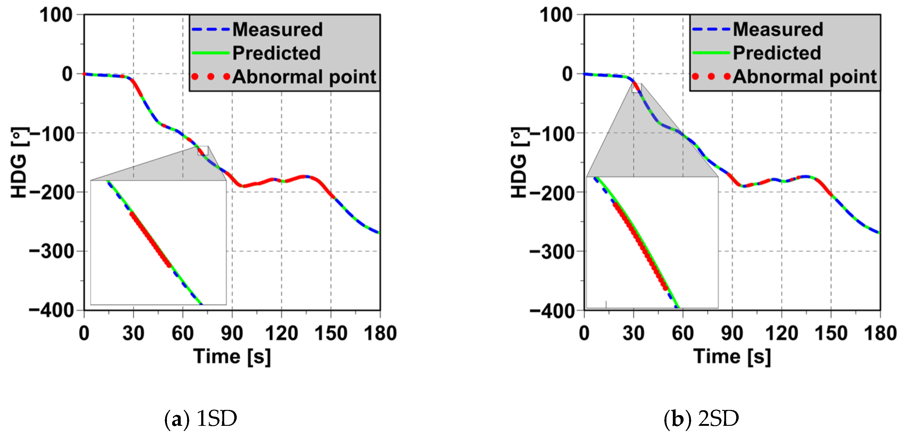
Figure 8 shows the abnormal detection results for HDG. At the 1SD threshold (0.296°), 605 abnormal points (33.799%) were detected, mainly during sharp turns at around 30 s, and from 90 s to 150 s. These may include natural heading changes. At 2SD (0.592°), the number of abnormal points decreased to 253 (14.134%), indicating improved selectivity for more sudden heading variations. At 3SD (0.888°), only the most significant heading anomalies were identified, with 109 points (6.089%) being detected. These points only exist around 90 s and 140 s, at which the heading angle suddenly decreased. Figure 8d shows that most values were under 2SD, with a few exceeding 3SD.

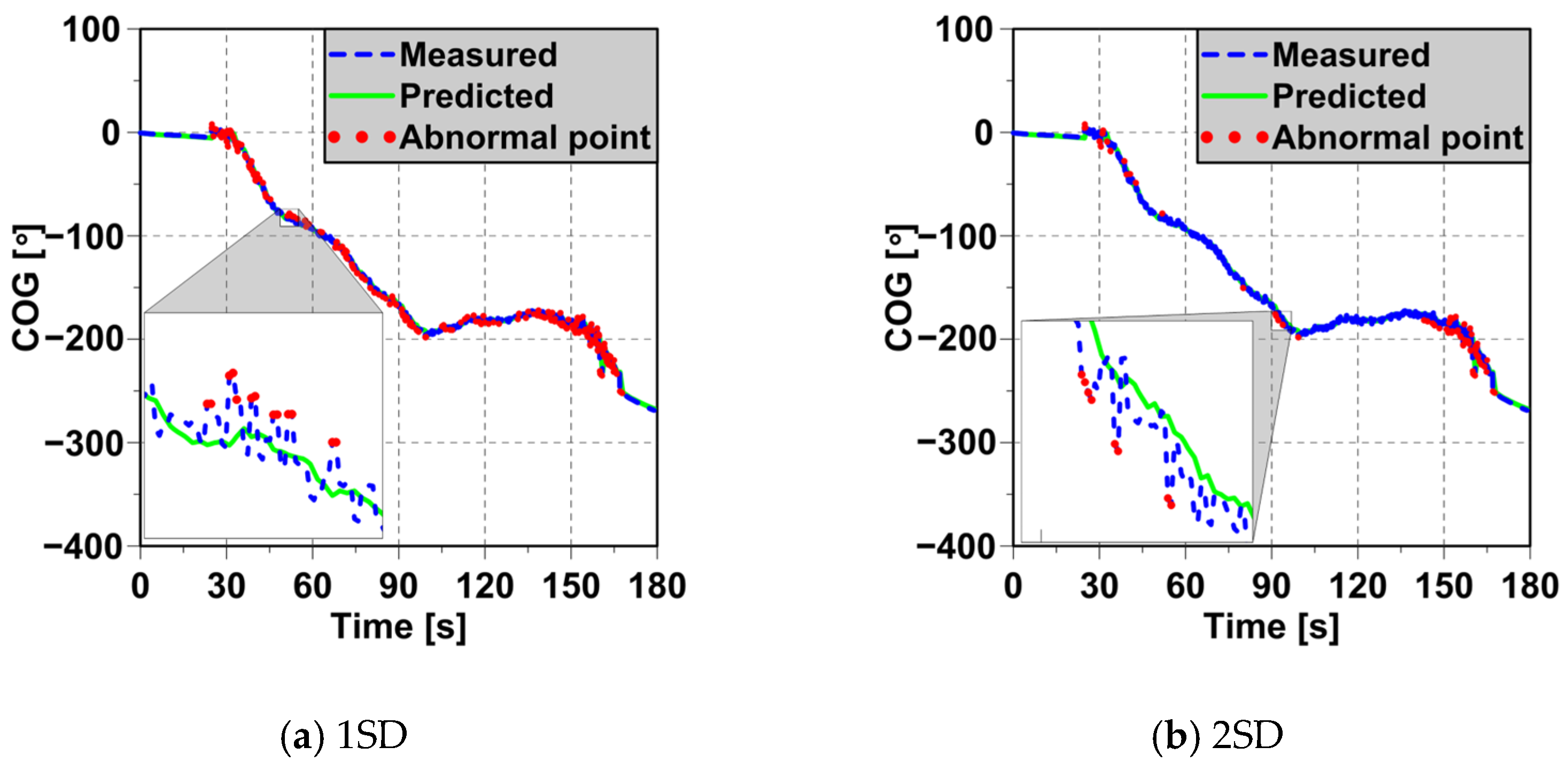
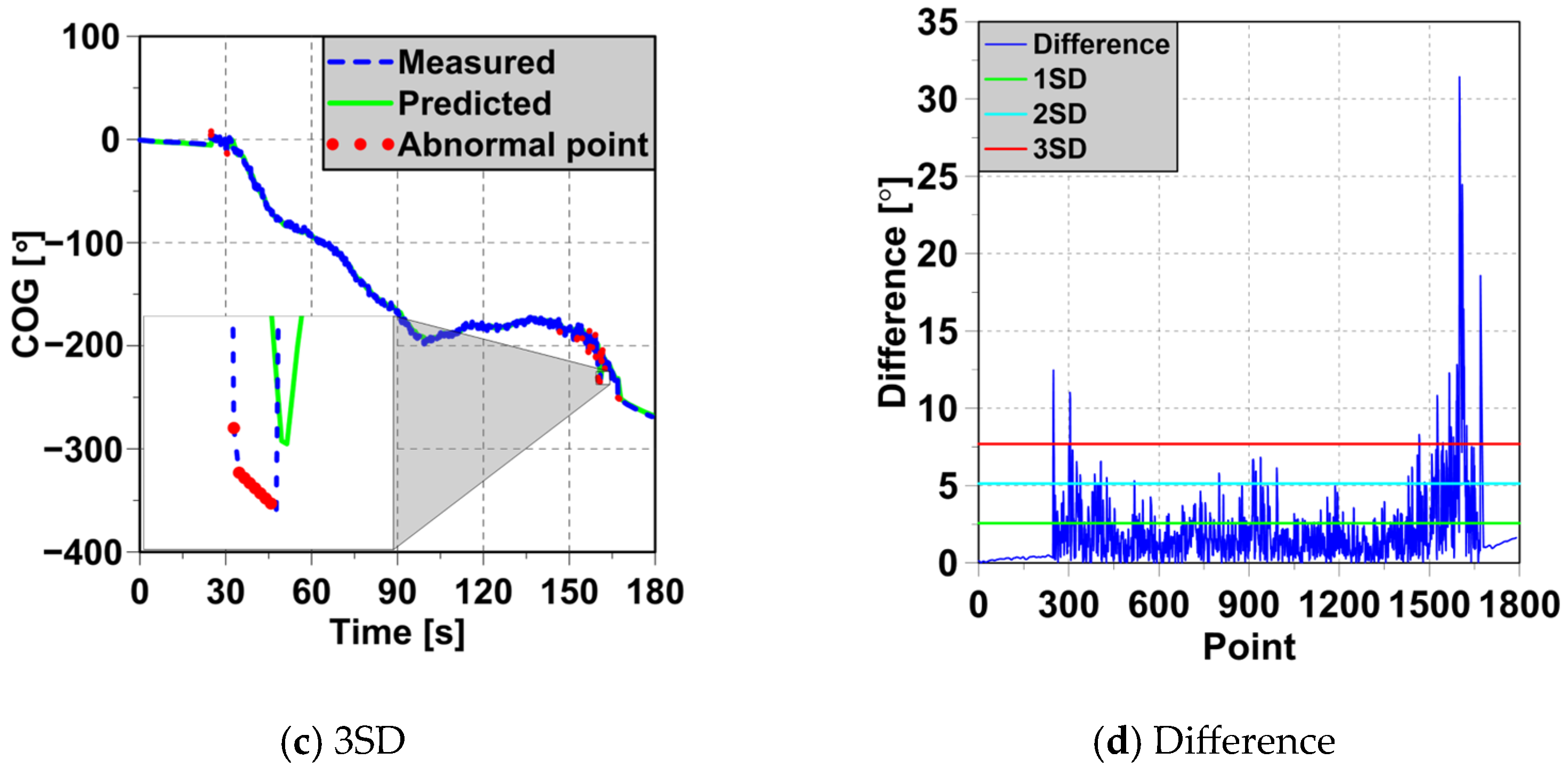
For COG (Figure 9), detection with a 1SD threshold (2.568°) resulted in 377 abnormal points (21.061%), spread between 30 s and 170 s. This wide distribution suggests small fluctuations and sensor noise. When the threshold was increased to 2SD (5.128°), the number of abnormal points significantly decreased to 121 points (6.760%), which were concentrated during sharp directional changes around 30, 90, and 160 s. At the 3SD threshold (7.692°), the detection became more selective, with only 44 points (2.458%) classified as abnormal points. Figure 9d confirms that most values were below 2SD, with higher thresholds reducing false positives.

In the case of SOG (Figure 10), 858 abnormal points (47.933%) were found at 1SD (0.0045 m/s), including both slow and fast speed changes. When the threshold was increased to 2SD (0.0090 m/s), the number of abnormal points decreased to 272 points (15.196%), mainly during acceleration or deceleration. At the highest threshold of 3SD (0.0135 m/s), only 85 points (4.749%) were detected, focusing on major speed changes. Figure 10d shows that most prediction errors stayed within 2SD.

The results across all four parameters (i.e., trajectory, HDG, COG, and SOG) show a consistent pattern: when using a low threshold (1SD) the detector becomes less selective, identifying numerous fluctuations, and potentially categorizing normal behavior as abnormal. As the threshold increases to 2SD and 3SD, abnormal detections become progressively more selective, capturing only substantial deviations from normal behavior. Statistically, using the 3SD threshold encompasses approximately 99.7% of the data in a normal distribution, meaning that only about 0.3% of points are expected to fall outside this range. This provides a strong quantitative basis for distinguishing true anomalies from normal behavior or sensor-induced noise. In this study, the 3SD level was therefore adopted as the final threshold, effectively reducing the number of detected points to around 2−10% and filtering out random fluctuations while retaining selectivity for significant deviations. Similar thresholds have also been adopted by Nie et al. [5] and Shi et al. [6], confirming that 3SD provides a practical balance between robustness of detection and operational reliability.

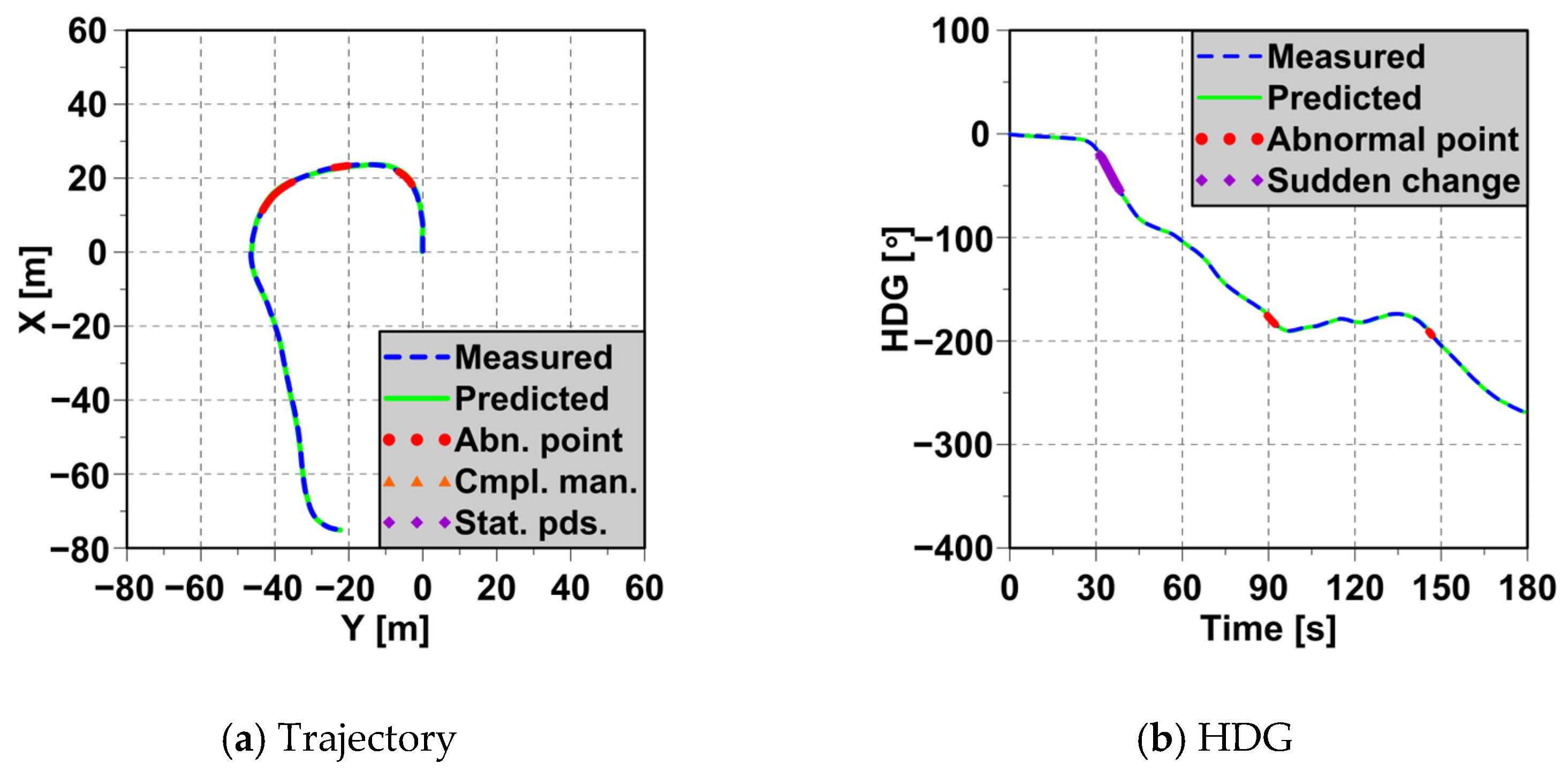
In the second stage, a direct abnormal behavior detection approach was applied to the sea trial data, independently of any predictive modeling. For the trajectory, abnormal behavior was identified based on three conditions: abnormal deviation (determined using the 3SD threshold), complex maneuvers, and stationary periods. The threshold for complex maneuvers was obtained from a free-running model test conducted in the square wave tank at Changwon National University, South Korea. In that test, a model-scale leisure boat performed a standard turning circle maneuver with a 35° rudder angle and a speed of 2 kn. The steady yaw rate reached approximately 13.041°/s, which represents the hydrodynamic limit of stable turning motion. Although this value was derived from a model test, it reflects the dynamic characteristics of model-scale displacement-type boats operating at similar Froude numbers. In this study, this value was used as a reference benchmark to distinguish normal maneuvers from excessive or unstable yaw motion during the sea trial. Currently, there are no regulatory criteria (from the International Maritime Organization, the International Association of Marine Aids to Navigation and Lighthouse Authorities, or port authorities) defining a fixed stop duration for the identification of stationary or abnormal behaviors in leisure boats. Such definitions typically depend on the specific application context, such as traffic analysis, anomaly detection, or port operation monitoring. In this study, stationary periods were considered as instances where the boat remained within a 1 m radius for more than 5 s during maneuvering. The threshold for sudden acceleration and deceleration was derived statistically from the SOG time-series data. Specifically, the value of 0.0723 m/s corresponds to 3SD of the consecutive SOG variations. This approach captures only the most significant changes in speed while filtering out random variations caused by environmental effects or sensor noise. Therefore, a threshold of 0.0723 m/s was taken to represent the upper limit of normal acceleration or deceleration, as observed during the sea trial, beyond which the behavior was flagged as abnormal points.

Figure 11 presents the abnormal detection results based on the established criteria, with corresponding thresholds and the number of detected abnormal points summarized in

Table 3. Abnormal detection results based on the established criteria.

Item	Threshold Value	Abnormal Points
Trajectory
Abnormal deviation	0.408 m	183
Complex maneuver	13.041°/s	0
Stationary period	1 m, 5 s	0
HDG
Sudden change	0.471°	65
COG
Sudden change	7.113°	32
SOG
Sudden acceleration	0.0723 m/s	12
Sudden deceleration		6

. Figure 11a shows the trajectory-based anomalies, where most of the 183 abnormal points were attributed to abnormal deviation, while no complex maneuvers or stationary periods were detected. Figure 11b illustrates the abnormal detection results for HDG, identifying 65 abnormal points, primarily during sharp directional changes that suggest potential control instability. In Figure 11c, 32 abnormal COG points were found using a 7.113° threshold, typically occurring during segments with multiple turns or steering actions. Finally, Figure 11d shows the abnormal SOG, where 12 sudden accelerations and 6 sudden decelerations were detected using a 0.0723 m/s threshold, likely caused by control inputs, environmental disturbances, or sensor noise.

4.4. Evaluation Based on Abnormal Behavior Criteria

To validate the abnormal behavior detection framework in a real-world context, the results were evaluated against a set of predefined abnormal behavior criteria, as summarized in

Table 4. Evaluation of criteria for abnormal ship behavior.

Criteria	Evaluation
Sudden speed changes	Satisfied
Unusual course changes	Satisfied
Extended stationary periods	Unsatisfied
Deviation from the expected route	Satisfied
Complex maneuvers	Unsatisfied
Track continuity issues	Unsatisfied

. The term “satisfied” indicates that the corresponding abnormal type was present in the sea trial data and successfully detected by the framework, while “unsatisfied” denotes that the anomaly type was not observed in the dataset. The framework successfully detected three types of abnormal behavior: sudden speed changes, unusual course changes, and deviations from the expected route. These results demonstrate that the proposed method effectively detects unexpected or abnormal ship behaviors. However, no extended stationary periods or complex maneuvering were present in the sea trial data and, thus, these anomaly types were marked as “unsatisfied.” Track continuity issues, such as missing data, also did not occur as the dataset was complete. In summary, all observable anomalies were correctly detected. However, the missing types highlight the need for future tests under more diverse operational conditions to comprehensively assess the system’s performance.

5. Conclusions

The primary objective of this study was to develop and validate an abnormal detection framework for ship behavior during sea trials. The proposed method integrates neural network-based prediction and statistical detection methods for enhanced accuracy and reliability.

In the first stage, a Long Short-Term Memory (LSTM) neural network was trained on real sea trial data to predict normal ship behavior. The model’s predicted values were compared with measured data, and large deviations were considered as potential abnormal behaviors. Three threshold levels were tested for the abnormal detection in trajectory, heading (HDG), course over ground (COG), and speed over ground (SOG). The third level (3SD) was chosen in order to capture only the most extreme cases, accounting for only 2−10% of the total data, indicating that false alarms caused by small errors or sensor noise were partially reduced with this threshold.

In the second stage, abnormal detection was performed directly on the sea trial data using practical criteria and the same 3SD threshold. Complex maneuvers were identified using a yaw rate threshold of 13.041°/s (based on a free-running model test), while stationary periods were detected when the boat remained within a 1 m radius for at least 5 s. Most detected abnormalities occurred in curved segments of the trajectory, where the boat performed sharp turns.

A checklist-based evaluation was applied to assess the framework’s performance. The system successfully detected multiple types of abnormal behavior, including sudden speed changes, unusual course deviations, extended stationary periods, and deviation from the expected route. These results confirm that combining predictive modeling with statistically determined thresholds provides a practical and robust approach for detecting abnormal ship behaviors. The successful validation of the proposed framework on real sea trial data demonstrates its potential for utilization in safety evaluation, system testing, and operational monitoring in autonomous or semi-autonomous ships.

Although this study successfully demonstrated the feasibility of the proposed abnormal detection framework for ship behavior, it has certain limitations. The current framework focuses on general abnormal detection and does not yet differentiate between true abnormal behaviors and false alarms arising from sensor noise, environmental disturbances, or operational variability. Moreover, the evaluation was conducted using a specific sea trial dataset, which may not fully represent the wide range of conditions encountered in real maritime operations. Future research will therefore aim to enhance the framework’s robustness and adaptability by testing it under diverse environmental and operational scenarios, including varying sea states, wind, and traffic conditions. The established detection thresholds and criteria will be further refined through additional sea trials, conducted with a real vessel at a marina port. This process will allow for iterative adjustment of the parameters through trial-and-error tuning, guided by empirical feedback from real-time performance. Such iterative validation is expected to help optimize the threshold settings and improve the model’s capability to distinguish genuine abnormal behaviors from measurement or environmental noise.

References

1. Kim, B.R.; Park, Y.K. ArcGIS based Analysis of Multiple Accident Areas Caused by Marine Plastic Litter in Republic of Korea. Appl. Chem. Eng. 2022, 33, 408–418. [Google Scholar]
2. Wang, Y.; Liu, J.; Liu, R.W.; Liu, Y.; Yuan, Z. Data-driven methods for detection of abnormal ship behavior: Progress and trends. Ocean Eng. 2023, 271, 113673. [Google Scholar] [CrossRef]
3. Ksciuk, J.; Kuhlemann, S.; Tierney, K.; Koberstein, A. Uncertainty in maritime ship routing and scheduling: A Literature review. Eur. J. Oper. Res. 2023, 308, 499–524. [Google Scholar] [CrossRef]
4. Baig, M.; Lagdami, K.; Mejia, M. Enhancing maritime safety: A comprehensive review of challenges and opportunities in the domestic ferry sector. Marit. Technol. Res. 2024, 6, 268911. [Google Scholar] [CrossRef]
5. Nie, Y.; Song, D.; Wang, Z.; Huang, Y.; Yang, H. Design and Motion Performance Analysis of Turbulent AUV Measuring Platform. Sensors 2022, 22, 460. [Google Scholar] [CrossRef] [PubMed]
6. Shi, Y.; Long, C.; Yang, X.; Deng, M. Abnormal Ship Behavior Detection Based on AIS Data. Appl. Sci. 2022, 12, 4635. [Google Scholar] [CrossRef]
7. Zhang, B.; Ren, H.; Wang, P.; Wang, D. Research Progress on Ship Anomaly Detection Based on Big Data. In Proceedings of the IEEE 11th International Conference on Software Engineering and Service Science (ICSESS), Beijing, China, 16–18 October 2020; pp. 316–320. [Google Scholar]
8. Rong, H.; Teixeira, A.P.; Guedes Soares, C. Data mining approach to shipping route characterization and anomaly detection based on AIS data. Ocean Eng. 2020, 198, 106936. [Google Scholar] [CrossRef]
9. Radon, A.N.; Wang, K.; Glasser, U.; Wehn, H.; Westwell-Roper, A. Contextual verification for false alarm reduction in maritime anomaly detection. In Proceedings of the IEEE International Conference on Big Data (Big Data), Santa Clara, CA, USA, 29 October–1 November 2015; pp. 1123–1133. [Google Scholar]
10. Yan, R.; Wang, S. Study of Data-Driven Methods for Vessel Anomaly Detection Based on AIS Data. Smart Innov. Syst. Tecnol. 2019, 149, 29–37. [Google Scholar]
11. Iphar, C.; Ray, C.; Napoli, A. Data integrity assessment for maritime anomaly detection. Expert Syst. Appl. 2020, 147, 113219. [Google Scholar] [CrossRef]
12. Rong, H.; Teixeira, A.P.; Guedes Soares, C. A framework for ship abnormal behavior detection and classification using AIS data. Reliab. Eng. Syst. Saf. 2024, 247, 110105. [Google Scholar] [CrossRef]
13. Ma, Q.; Lian, S.; Zhang, D.; Lang, X.; Rong, H.; Mao, W.; Zhang, M. A machine learning method for the recognition of ship behavior using AIS data. Ocean Eng. 2024, 315, 119791. [Google Scholar] [CrossRef]
14. Sadeghi, Z.; Matwin, S. Anomaly detection for maritime navigation based on probalility density function of error of reconstruction. J. Intell. Syst. 2023, 32, 20220270. [Google Scholar]
15. Li, J.; Liu, J.; Zhang, X.; Li, X.; Wang, J.; Wu, Z. A Novel Hybrid Approach for Detecting Abnormal Vessel Behavior in Maritime Traffic. In Proceedings of the 7th International Conference on Transportation Information and Safety (ICTIS), Xi’an, China, 4–6 August 2023; pp. 1–7. [Google Scholar]
16. Lee, H.T.; Yang, H. Ship-Route Prediction Based on a Long Short-Term Memory Network Using Port-to-Port Trajectory Data. J. Mar. Sci. Eng. 2024, 12, 2241. [Google Scholar] [CrossRef]
17. Liu, R.W.; Hu, K.; Liang, M.; Li, Y.; Liu, X.; Yang, D. QSD-LSTM: Vessel trajectory prediction using long short-term memory with quaternion ship domain. Appl. Ocean Res. 2023, 136, 103592. [Google Scholar] [CrossRef]
18. Guo, Z.; Qiang, H.; Peng, X. Vessel Trajectory Prediction Using Vessel Influence Long Short-Term Memory with Uncertainty Estimation. J. Mar. Sci. Eng. 2025, 13, 353. [Google Scholar] [CrossRef]
19. Wang, C.; Fu, Y. Ship Trajectory Prediction Based on Attention in Bidirectional Recurrent Neural Networks. In Proceedings of the 5th International Conference on Information Science, Computer Technology and Transportation (ISCTT), Shenyang, China, 13–15 November 2020; pp. 529–533. [Google Scholar]
20. Sun, Q.; Tang, Z.; Gao, J.; Zhang, G. Short-term ship motion attitude prediction based on LSTM and GPR. Appl. Ocean Res. 2022, 118, 102927. [Google Scholar] [CrossRef]
21. Zaman, U.; Khan, J.; Lee, E.; Hussain, S.; Balobaid, A.S.; Aburasain, R.Y.; Kim, K. An Efficient Long Short-Term Memory and Gated Recurrent Unit Based Smart Vessel Trajectory Prediction Using Automatic Identification System Data. Comput. Mater. Contin. 2024, 81, 1789–1808. [Google Scholar] [CrossRef]
22. Yang, S.; Xinya, P.; Zexuan, D.; Jiansen, Z. An Approach to Ship Behavior Prediction Based on AIS and RNN Optimization Model. Int. J. Transp. Eng. Technol. 2020, 6, 16–21. [Google Scholar] [CrossRef]
23. Wolsing, K.; Roepert, L.; Bauer, J.; Wehrle, K. Anomaly Detection in Maritime AIS Tracks: A Review of Recent Approaches. J. Mar. Sci. Eng. 2022, 10, 112. [Google Scholar] [CrossRef]
24. Ying, W.; Ou, M.; Liang, Q.; Yang, Z.; Zhao, M. Abnormal Detection Method of Transship Based on Marine Target Spatio-Temporal Data. J. Internet Technol. 2023, 24, 1123–1130. [Google Scholar] [CrossRef]
25. Tyasayumranani, W.; Hwang, T.; Hwang, T.; Youn, I.H. Anomaly detection model of small-scaled ship for maritime autonomous surface ships’ operation. J. Int. Marit. Saf. Environ. Aff. Shipp. 2022, 6, 224–235. [Google Scholar] [CrossRef]
26. Zhang, B.; Hirayama, K.; Ren, H.; Wang, D.; Li, H. Ship Anomalous Behavior Detection Using Clustering and Deep Recurrent Neural Network. J. Mar. Sci. Eng. 2023, 11, 763. [Google Scholar] [CrossRef]
27. Li, G.; Zhang, X.; Shu, Y.; Wang, C.; Guo, W.; Wang, J. Ship Anomalous Behavior Detection in Port Waterways Based on Text Similarity and Kernel Density Estimation. J. Mar. Sci. Eng. 2024, 12, 968. [Google Scholar] [CrossRef]
28. Yang, B. A mathematical investigation on the distance-preserving property of an equidistant cylindrical projection. arXiv 2021. [Google Scholar] [CrossRef]
Figure 1. Leisure boat.
Jmse 13 02391 g001
Figure 2. Sea trial data (raw data).
Jmse 13 02391 g002
Figure 3. Sea trial data (processed data).
Jmse 13 02391 g003
Figure 4. Validation losses of LSTM model architectures under different numbers of training epochs.
Jmse 13 02391 g004
Figure 5. Training and validation loss curves for the LSTM model with architecture [128,128] over 40 epochs.
Jmse 13 02391 g005
Figure 6. Normal ship behavior predicted using an LSTM model.
Jmse 13 02391 g006aJmse 13 02391 g006b
Figure 7. Abnormal points in the trajectory by threshold levels.
Jmse 13 02391 g007
Figure 8. Abnormal points in HDG by threshold levels.
Jmse 13 02391 g008aJmse 13 02391 g008b
Figure 9. Abnormal points in COG by threshold levels.
Jmse 13 02391 g009aJmse 13 02391 g009b
Figure 10. Abnormal points in SOG by threshold levels.
Jmse 13 02391 g010
Figure 11. Abnormal detection results based on the established criteria.
Jmse 13 02391 g011aJmse 13 02391 g011b