A Matheuristic Framework for Behavioral Segmentation and Mobility Analysis of AIS Trajectories Using Multiple Movement Features

Abstract

Accurate behavioral segmentation of vessel trajectories from Automatic Identification System (AIS) is essential for maritime safety and traffic management. Existing methods often rely on predefined thresholds or emphasize geometric criteria and offer limited behavioral interpretability for mobility analysis. This paper introduces an unsupervised behavioral segmentation framework that integrates clustering with matheuristic optimization. Trajectories are cleaned with a forward sliding window, and three smoothed movement features, namely speed, acceleration, and turning rate, are computed for each point. Each feature is discretized by the Jenks Natural Breaks algorithm to extract key feature points and pointwise feature labels. Segment boundaries are near-optimally chosen from these key feature points using a Matheuristic Fixed Set Search (MFSS) that minimizes a Minimum Description Length (MDL) objective. This ensures behavioral consistency within each segment and clear separation between adjacent segments. Experiments on an AIS dataset from the Qiongzhou Strait, China, demonstrate that our proposed method yields more compact, distinctly differentiated segments than baseline methods, while preserving intra-segment behavioral continuity. These segments exhibit strong semantic coherence, making them well-suited for downstream tasks such as traffic risk assessment and route planning.

1. Introduction

The Automatic Identification System (AIS) is a tracking system used for collision avoidance and traffic management. According to the SOLAS regulation V/191, AIS is required to be fitted aboard all ships of 300 gross tonnage and upwards engaged on international voyages, cargo ships of 500 gross tonnage and upwards not engaged on international voyages, and all passenger ships irrespective of size. This system enables vessels to periodically broadcast their identity, position, and kinematic status to nearby vessels, shore stations, and satellites. The widespread adoption of AIS technology has led to an increasing availability of vessel trajectory data, substantially expanding opportunities for maritime research, including anomaly detection [1], trajectory prediction [2], traffic safety evaluation [3], shipping route modeling [4], automatic routing [5], waterway capacity estimation [6], and cargo operation analysis [7]. The effectiveness of these applications depends on the appropriate processing and interpretation of trajectory data, among which trajectory segmentation serves as one of the most essential processing steps for trajectory data mining [8].

Trajectory segmentation aims to divide continuous trajectories into meaningful sub-trajectories by detecting change points in spatial, temporal, or behavioral attributes. Existing research can be grouped into two main categories based on its segmentation criteria. The first group comprises shape-based methods, which analyze the geometric structure of trajectories and identify segments according to spatial and temporal properties. The second one includes behavior-based methods, where trajectories are divided into segments with homogeneous kinematic features such as speed, acceleration and heading [9,10]. Within behavior-based segmentation, some studies focused on identifying specific behaviors, particularly stop and move [11,12], while others pursued pattern-driven discovery of multiple behavior classes [13].

From a methodological perspective, most trajectory segmentation methods can be classified as supervised or unsupervised [14]. Supervised approaches typically use preset thresholds on trajectory attributes such as distance or speed to guide the segmentation process [15,16]. For labeled datasets [17], pretrained models can also be applied to identify segments with the same labels [18,19]. In contrast, unsupervised segmentation methods identify segments based on inherent similarities or distribution patterns within trajectory data instead of preset thresholds. Common unsupervised strategies include clustering-based methods that adapt or extend algorithms such as K-Means and DBSCAN for AIS trajectory segmentation [20], objective-based methods that employ criteria like the Minimum Description Length (MDL) principle to achieve compact and meaningful trajectory representations [13], and interpolation-based methods that identify change points by comparing interpolated and observed trajectory points [21].

Despite considerable progress in trajectory segmentation, several methodological and data-related challenges remain unresolved. First, the choice of segmentation criterion strongly affects downstream behavior analysis. For example, segmentation methods using distance thresholds may divide a continuous turning maneuver into several fragments due to large positional deviations between successive points, while sequences of acceleration and deceleration along straight paths may be grouped into a single segment because of limited spatial variation, thereby disrupting the integrity of complete behaviors and limiting the utility of shape-based approaches for behavior-sensitive applications [22]. Second, the choice of segmentation method also introduces limitations. Supervised methods provide interpretable results through predefined rules or labeled samples, but are sensitive to threshold selection and data anomalies, thus reducing generalizability and robustness [23]. Among unsupervised methods, clustering-based approaches often struggle to effectively segment trajectories with multiple behavioral attributes, while objective-based and interpolation-based approaches may lack interpretability. Finally, AIS trajectory data itself presents unique challenges that reinforce these algorithmic limitations. Unlike moving objects on land such as vehicles or pedestrians, vessels navigate with higher degrees of freedom in open waterways without rigid infrastructure constraints and display less distinct behavioral patterns due to limited maneuverability. Moreover, AIS data are prone to inconsistencies and errors resulting from the disruption between multiple data receivers and environmental influences such as wind, waves, and currents. Therefore, improving the generalizability, robustness, and interpretability of segmentation algorithms remains a major focus for current research.

To bridge the above research gaps, this study proposes an unsupervised clustering-aided matheuristic framework for behavioral segmentation of AIS trajectories. Trajectories are first preprocessed with a forward sliding window procedure to remove outliers and generate smoothed profiles of speed, acceleration, and turning rate. These continuous profiles are then discretized into distinct feature labels using the Jenks Natural Breaks algorithm, and key feature points are extracted as candidate segment boundaries where label changes occur. The segmentation is formulated as an optimization problem that divides trajectories at these boundaries by minimizing the MDL to balance intra-segment homogeneity and inter-segment distinctness. To solve this problem systematically and efficiently, the problem is reformulated at the segment level and a Matheuristic Fixed Set Search (MFSS) framework is employed with a Greedy Randomized Top-Down (GRTD) initialization. The final output divides trajectories into behaviorally coherent segments characterized by consistent semantic classes derived from dominant feature labels from Jenks decomposition.

The main contributions of this paper are summarized as follows:

• A behavior-based segmentation approach is introduced using speed, acceleration, and turning rate, where turning rate captures geometric variation without relying on distance thresholds. Each behavioral attribute is discretized independently using Jenks algorithm, which reduces interference among attributes and provides interpretable feature labels for subsequent behavioral analysis. Furthermore, key feature points, identified by label differences between consecutive trajectory points, narrow the candidate set of segmentation boundaries and thereby accelerate the subsequent optimization process.
• To enhance generalizability across vessels of varying sizes and to adapt to the noisy and irregular characteristics of AIS data, the MDL principle is employed as the segmentation objective. This formulation ensures consistent multi-attribute segmentation with movement features normalized by their respective maximum values and enables the discovery of diverse navigation patterns.
• A MFSS algorithm is developed to achieve an effective balance between segmentation accuracy and computational efficiency. The framework incorporates a segmentwise reformulation of the problem to linearize MDL terms and mitigate sensitivity to isolated point fluctuations, a random fixed set for global exploration, a mixed-integer programming (MIP) solver for local refinement, and the GRTD initialization to generate high-quality candidate solutions.

The rest of this paper is organized as follows. Section 2 reviews related work on trajectory segmentation and behavioral analysis. Section 3 introduces the proposed framework in detail. Section 4 presents the experimental results and behavioral segment visualizations based on a case study in the Qiongzhou Strait. Finally, Section 5 concludes the paper and discusses directions for future research.

2. Related Work

Trajectory segmentation aims to divide continuous trajectories into meaningful sub-trajectories by detecting change points in spatial, temporal, or behavioral attributes using supervised or unsupervised methods. In this section, shape-based segmentation methods considering spatial–temporal continuity are first reviewed, distinguishing between supervised and unsupervised approaches. The discussion then focuses on behavior-based segmentation, covering both semantics-guided methods that target specific activities and pattern-driven methods that identify and interpret diverse behavioral patterns.

Supervised methods rely on predefined thresholds such as time, speed, density, or direction to guide partitioning processes. Common time-series strategies include top-down using Douglas-Peucker (DP) [24], bottom-up, and sliding window algorithm that locate breakpoints where attribute variations exceed preset thresholds. Liu et al. [16] employed the DP algorithm to partition vessel tracks into short non-overlapping segments via distance-based feature points for subsequent matching. Ma et al. [25] detected critical turns with an Open Window procedure and directional thresholds to preserve geometric motion features. Another approach formalized criteria combining speed, heading, and curvature within greedy sequential frameworks to generate homogeneous segments [15]. Hybrid methods integrate multiple strategies, such as the SWAB (Sliding Window and Bottom-up) [26] algorithm to deliver near-offline segmentation quality in streaming settings. Lin et al. [27] integrated Kalman filtering, Douglas-Peucker simplification, and sliding window corner detection to obtain noise-robust, behaviorally consistent segments. Amigo et al. [28] systematically compared multiple supervised algorithms and revealed that parameter choices like distance thresholds and window sizes strongly shape segment structures. Supervised trajectory segmentation methods are efficient when domain knowledge is available for parameter calibration. However, their reliance on manually tuned thresholds and sensitivity to parameter variations limit their generalizability across diverse application scenarios.

Unsupervised segmentation identifies segments based on inherent similarities or distribution patterns within trajectory data by employing various underlying methods or mechanisms. Clustering-based methods adapt algorithms such as K-Means and DBSCAN to enforce spatiotemporal continuity. For instance, Warped K-Means [29] incorporates sequential constraints to generate temporally ordered segments, while ST-DBSCAN [30] and T-DBSCAN [31] extend density-based clustering by integrating spatial, temporal, and non-spatial attributes to identify homogeneous movement patterns under varying conditions. Objective-based methods typically employ cost functions such as the MDL [32] to achieve compact and meaningful trajectory representations. For example, TRACLUS [33] applies the MDL principle to partition trajectories into line segments and then clusters similar segments to extract frequent movement patterns. Interpolation-based methods enhanced adaptability by identifying change points through deviation analysis between observed and interpolated trajectories. Etemad et al. [34] introduced Octal Window Segmentation (OWS), which detected behavioral transitions by comparing observed positions with interpolated estimates within a sliding window, and subsequently extended this framework into Sliding Window Segmentation (SWS) [21] by integrating multiple interpolation kernels and bidirectional estimation to improve robustness and precision. Although unsupervised segmentation methods often delivered segments with high internal consistency and generalizability, they still exhibited limited interpretability and reduced capability for capturing multi-attribute behavioral patterns.

Compared with methods that emphasize spatial or geometric continuity, behavior-based trajectory segmentation aims to partition trajectories into semantically coherent segments that reflect underlying activities. These approaches comprise semantics-guided segmentation using predefined behaviors and pattern-driven segmentation discovering intrinsic movement patterns. Representative semantics-guided work concentrates on stop-move detection and several approaches incorporate external information for enhanced interpretability. The Stops and Moves of Trajectories (SMoT) [11] framework detects stops by intersecting trajectories with geographic objects, while the Hierarchical-Graph-based Similarity Measurement (HGSM) [35] clusters stay points hierarchically to construct user location histories. Similarly, Guo et al. [36] modeled trajectory segmentation as a probabilistic logic optimization problem that integrates dwell times, business schedules, and electronic fences to infer activity types in logistics scenarios. In contrast, methods relying solely on trajectory data include Clustering-Based SMoT (CB-SMoT) [12], Sequence Oriented Clustering (SOC) [37], and semantics-based simplification [38], which identify stops and moves by integrating spatiotemporal density and speed features under noisy conditions.

While trajectory segmentation for humans and vehicles typically reflects deliberate movements constrained by infrastructure, vessel motion is often influenced by environmental forces such as wind, waves, and currents, leading to passive or unintentional displacements. For instance, vessels at anchor or berth may drift without active navigation control, introducing ambiguity into segmentation and behavioral interpretation. To mitigate these effects in identifying stop and move status, recent studies have incorporated directional and shape features to enhance segmentation robustness and semantic consistency. The Sevcik Trajectory Shape (STShp) [39] framework combines speed thresholds with time-weighted shape features, while other approaches integrate density-based clustering of directional features to identify stops and moves [40]. Beyond conventional stop–move segmentation, some studies aim to interpret the underlying causes of stationary behaviors, such as fishing-induced stops. The Direction-Based SMoT algorithm (DB-SMoT) [41] detects fishing activities through directional consistency rather than speed, and the Window-Based Segmentation with Run-Length Encoding method (WBS-RLE) [42] employs window-based classification to identify complete fishing segments. To better adapt to domain-specific behavioral characteristics, semi-supervised approaches have also been introduced. Etemad et al. [18] extended OWS [34] by training a classifier on labeled fishing data to detect segment boundaries, while Soares Júnior et al. [19] proposed RGRASP-SemTS, a semi-supervised extension of the unsupervised segmentation algorithm GRASP-UTS [13], which refines MDL-based segmentation through reactive greedy randomized search using both labeled and unlabeled trajectories.

Multi-behavior segmentation methods extend beyond single-behavior detection to identify diverse activity patterns within trajectories. Representative approaches include state-based bottom-up frameworks using machine learning to classify fixed-length segments into various activity states [43], the Semantic Enrichment Process for Spatiotemporal trajectories based on Semantic Information Matching framework (SEPSIM) [44] combining DBSCAN segmentation with semantic matching, and SEMANTIC-SEG [45] integrating change-point detection with ontology reasoning to annotate segments with multiple labels. In maritime applications, ontology-enhanced dynamic Bayesian networks segment ship behaviors across harbor scenes [46], while navigation state-based methods partition trajectories by operational modes beyond mooring and sailing [47]. Although these semantics-guided methods effectively recognize predefined activity types, they typically cannot identify patterns beyond their established label sets.

In contrast to segmentation with predefined behaviors, pattern-driven approaches focus on identifying homogeneous segments based on inherent behavioral patterns, where each segment exhibits internal consistency while differing from adjacent ones. Methods like FLOSS [48] use matrix profiles to detect regime changes in time series without domain-specific parameters. Feature-based techniques, proposed by Izakian et al. [9], extract multiple movement parameters via sliding windows and cluster them into coherent segments. Xu and Dong [49] combined multi-feature similarity with an MDL-based merging step in TS-MF to avoid over-segmentation and maintain low parameter dependence. Although these approaches produced internally consistent segments, they provided limited semantic labels. To improve interpretability, several studies combined unsupervised segmentation with semantic modeling. For instance, Li et al. [50] and Huang et al. [51] applied topic models to segmented ship trajectories, encoding them into semantic patterns for interpretable behavior recognition and mobility analysis.

Despite considerable advances in trajectory segmentation, current methods remain challenged by both algorithmic limitations and the complexity of AIS trajectories. Supervised approaches rely on manually tuned thresholds or domain-specific rules, which provide efficiency under careful threshold calibration but limit generalization across vessel types and operational contexts. Unsupervised methods present their own challenges, as clustering-based techniques often produce fragmented segments due to parameter sensitivity and multi-dimensional feature diversity, while interpolation-based approaches are highly sensitive to the errors between predicted values and extreme values. Objective-based methods such as MDL can balance intra-segment consistency and inter-segment distinctiveness, yet they often incur high computational costs and provide limited semantic interpretability. These challenges are further amplified by the high-dimensional, noisy, and discontinuous nature of real AIS trajectories and by environmental or operational fluctuations that disrupt behavioral patterns and destabilize pointwise segmentation. These limitations motivate our matheuristic-based behavioral segmentation framework, which integrates a pre-clustering step to identify key change points and support semantic interpretability, a normalized MDL formulation to handle multi-dimensional features and the complexity of AIS trajectories, and a matheuristic search strategy that balances solution quality with computational efficiency.

3. Matheuristic-Based Behavioral Segmentation

3.1. Basic Definitions

Definition 1

(Trajectory Point Set P). A trajectory consists of a temporally ordered sequence of points $p_i=[(x_i,y_i),h_i,s_i,a_i,r_i,t_i]$, where the attributes represent planar coordinates, heading, speed, acceleration, turning rate, and timestamp, respectively. To enable behavioral comparison, each point is augmented with normalized kinematic variables ${\tilde{s}}_i,{\tilde{a}}_i,{\tilde{r}}_i$. These normalized values are used consistently throughout the evaluation metrics.

Definition 2

(Candidate Boundary Set $C_p$). Based on the decomposition of the normalized feature profiles, we identify three key feature point sets $K_s,K_a,K_r$ corresponding to speed, acceleration, and turning rate changes. The candidate boundary set is defined as the union $C_p=K_s\cup K_a\cup K_r$, containing all points eligible to serve as segment boundaries.

Definition 3

(Segment Set $\widehat{S}$). The trajectory is partitioned into contiguous segments $\widehat{S}=\{S_1,\dots ,S_m\}$. Each segment $S_k$ spans from start point $p_u^k$ to end point $p_v^k$, where $p_v^k\equiv p_u^{k+1}$ to ensure continuity. Each segment is characterized by a behavioral centroid $c_k=({\tilde{s}}_k^c,{\tilde{a}}_k^c,{\tilde{r}}_k^c)$, computed as the average of normalized attributes within $S_k$. Additionally, a behavioral class is assigned to $S_k$ based on the dominant point labels derived from the decomposition.

Definition 4

(Behavioral Metrics). To quantify segmentation quality in the behavioral feature space, we define:

• Feature Dissimilarity $D(p_i,p_j)$: The Euclidean distance between two points in the normalized feature space:

  $$D(p_i,p_j)=\sqrt{{({\tilde{s}}_i-{\tilde{s}}_j)}^2+{({\tilde{a}}_i-{\tilde{a}}_j)}^2+{({\tilde{r}}_i-{\tilde{r}}_j)}^2}.$$

  (1)
• Segment Cohesiveness $H\left(S_k\right)$: The behavioral homogeneity within a segment relative to its centroid:

  $$H\left(S_k\right)=\sum _{i=u}^{v}D(c_k,p_i^k).$$

  (2)
• Inter-segment Distinctness $D_s(S_k,S_{k+1})$: The dissimilarity between adjacent segment centroids:

  $$D_s(S_k,S_{k+1})=D(c_k,c_{k+1})=\sqrt{{({\tilde{s}}_k^c-{\tilde{s}}_{k+1}^c)}^2+{({\tilde{a}}_k^c-{\tilde{a}}_{k+1}^c)}^2+{({\tilde{r}}_k^c-{\tilde{r}}_{k+1}^c)}^2}.$$

  (3)

3.2. AIS Data Preprocessing

Unreliable or noisy data, such as sudden jumps caused by GPS errors or irregular changes in vessel speed, can negatively affect behavioral analysis. To address this, we implement a unified preprocessing framework based on a forward sliding window process. This approach integrates the detection of data discontinuities, redundancy, and physical anomalies within a shared localized context. By evaluating each trajectory point relative to its immediate history, the sliding window facilitates efficient and adaptive data cleaning.

Within the unified forward sliding window framework, we first address data discontinuities and redundancy before evaluating physical anomalies. To manage signal loss, the trajectory is divided into independent sub-trajectories whenever the time interval between consecutive points in the window exceeds a specified threshold. Subsequently, data redundancy is resolved by distinguishing between spatial and temporal duplication. Spatial duplicates are identified as records with identical coordinates occurring when the vessel speed is non-zero, a distinction necessary to preserve valid anchoring status. For these cases, the system retains only the earliest recorded entry. Regarding temporal conflicts where multiple distinct points share the same timestamp, validity is determined by assessing spatial continuity relative to the preceding and succeeding points. The observation that minimizes the Synchronous Euclidean Distance (SED) is preserved to ensure kinematic consistency.

For each sliding window, we implement a dual-check mechanism to identify geographic and behavioral anomalies. Geographic anomalies are detected using the SED, which quantifies the spatial deviation of a point relative to its neighbors. We calculate the average SED of preceding point triplets within the window to establish a local baseline for trajectory smoothness. The current observation is flagged as a positional outlier if the SED of the triplet involving the new point significantly exceeds this historical average. Simultaneously, behavioral anomalies are determined by monitoring the temporal rates of change in speed and heading. An observation is rejected if the variation rate in the current time interval surpasses the mean variation rate of preceding intervals within the window by a predefined threshold. This detection logic is formulated as:

$$\begin{array}{cc}\hfill \mathrm{Geographic}:& \mathrm{SED}(p_{i-1},p_{i-2},p_i)>{\theta }_g·{\displaystyle \frac{1}{W-2}}\sum _{k=2}^{W-1}\mathrm{SED}(p_{i-k},p_{i-k-1},p_{i-k+1})\hfill \\ \hfill \mathrm{Behavioral}:& {\Delta }_{rate}(p_{i-1},p_i)>{\theta }_b·{\displaystyle \frac{1}{W-1}}\sum _{k=1}^{W-1}{\Delta }_{rate}(p_{i-k-1},p_{i-k})\hfill \end{array}$$

(4)

where $\mathrm{SED}(b,a,c)$ denotes the synchronous euclidean distance of point b relative to the segment $ac$, and ${\Delta }_{rate}(a,b)$ represents the absolute rate of change (speed or heading) between points a and b normalized by time. ${\theta }_g$ and ${\theta }_b$ are the sensitivity thresholds for geographic and behavioral deviations, respectively.

3.3. Movement Feature Generation, Decomposition and Key Feature Point Extraction

The cleaned trajectory is used to compute the smoothed acceleration and turning rate using exponentially decaying weights, which prioritize points in close proximity to the current position. This approach effectively suppresses short-term fluctuations and enhances the robustness of the derived motion parameters. Acceleration and turning rate are calculated as the weighted average of local derivatives:

$$a_i=\sum _{w=1}^W{\mathrm{EXP}}_w{\displaystyle \frac{v_i-v_{i-w}}{t_i-t_{i-w}}},r_i=\sum _{w=1}^W{\mathrm{EXP}}_w{\displaystyle \frac{\parallel h_i-h_{i-w}\parallel }{t_i-t_{i-w}}}$$

(5)

Here, $v_i$ and $h_i$ represent the vessel speed and heading at time $t_i$, respectively. $\parallel h_i-h_{i-w}\parallel$ denotes the minimal angular difference between two headings, accounting for the circular nature of angles. The parameter ${\mathrm{EXP}}_w$ denotes the exponentially decaying weight applied to the $w^{th}$ preceding observation in the sliding window with window width W and decay rate $\lambda$, defined as:

$${\mathrm{EXP}}_w={\displaystyle \frac{e^{-\lambda w}}{{\sum }_{k=1}^W{e}^{-\lambda k}}}$$

(6)

This formulation smoothes short-term fluctuations caused by operational variability while preserving the intrinsic behavioral transitions along the trajectory. The sample of trajectory and its behavioral profiles are shown in Figure 1.

Key feature points (KFPs) are trajectory points at which one or more movement parameters exhibit a discrete class change. These points serve as candidate segment boundaries in the matheuristic-based segmentation, reducing computational complexity by limiting the search space and providing behavioral transitions.

Each parameter profile is decomposed into distinct classes using the Jenks method. This algorithm minimizes variance within classes and maximizes variance between classes, making it suitable for the heterogeneous distributions commonly observed in movement data [52]. A KFP is identified whenever the class assignment differs from that of the previous point.

The final set of candidate boundaries is obtained by aggregating KFPs across all parameter profiles. Since each movement parameter may reflect behavioral changes at different times, this aggregation ensures that segmentation captures all relevant transitions, leading to a more comprehensive and robust trajectory division.

An example of KFP extraction and aggregation is shown in Figure 2 and Figure 3. In Figure 2, Jenks algorithm decomposes the one-dimensional speed values into three classes so that within-class variance is small and between-class variance is large. The class boundaries are marked by the orange and red vertical lines and these boundaries induce four temporal segments along the trajectory. For each movement parameter (speed, acceleration, turning rate), the class change points from the corresponding Jenks decomposition are extracted as key feature points, here marked with circles, squares and triangles, respectively, in Figure 3. The three sets of key feature points are aggregated on the trajectory so that the temporal and spatial coincidence of changes is visible. The aggregation of these points forms the candidate boundaries used by the matheuristic algorithm, ensuring that segmentation accounts for changes detected in any movement attribute.

3.4. Problem Description

The matheuristic algorithm is used to partition the original trajectory into segments based on the KFPs provided in Section 3.3. The optimal segmentation should minimize distortion, ensuring high behavioral similarity within each segment, and maximize compression by reducing the total number of segments [13]. Considering the tradeoff between minimal distortion and maximal compression, the MDL principle is applied and the problem is formulated as an optimization procedure.

3.4.1. The MDL Principle

The MDL principle, proposed by Rissanen [32], provides a formal framework for selecting an optimal model by balancing model complexity and descriptive efficiency, particularly suitable for time series data. The optimal hypothesis is the one that minimizes the total code length required to describe both the model and the data under that model. Let H denote the hypothesis and D the dataset, the MDL objective can be expressed as:

$$\mathrm{MDL}=L\left(H\right)+L(D\mid H),$$

(7)

where $L\left(H\right)$ is the code length of the hypothesis in bits, and $L\left(D\right|H)$ is the code length of the data in bits when encoded according to H [53].

For trajectory segmentation, we adapt the MDL framework proposed by Soares Júnior et al. [13] to define our objective function. Specifically, we adopt the mechanism of using the maximum feature dissimilarity $M_{max}$ in the hypothesis cost $L\left(H\right)$ to normalize the description length. However, unlike previous approaches that utilize actual trajectory landmarks, we define the hypothesis H as the set of behavioral centroids ${\left\{c_k\right\}}_{k=1}^m$ to better represent the dominant behavioral characteristics of the segments $\widehat{S}=\{S_1,\dots ,S_m\}$. Consequently, $L\left(H\right)$ measures the cost of encoding these centroids. When adjacent centroids differ substantially in behavioral features, each can represent a larger region of the trajectory, allowing for fewer centroids and a more compressed representation. $L\left(D\right|H)$ captures the internal consistency within each segment by quantifying the behavioral difference between all points in a segment and their corresponding centroid, denoted as $H\left(S_j\right)$. The two MDL components are defined as:

$$L\left(H\right)={log}_2\left(1+\sum _{k=1}^{m-1}\left(M_{max}-D(c_k,c_{k+1})\right)\right),$$

(8)

$$L(D\mid H)={log}_2\left(1+\sum _{k=1}^{m}H\left(S_k\right)\right),$$

(9)

where $M_{max}$ is the maximum Euclidean distance between behavioral feature vectors, and the addition of 1 inside the logarithm ensures non-negativity.

By minimizing the MDL function through Equations (8) and (9), an optimal balance is achieved between the number of segments and the homogeneity of points within each segment. Treating the entire trajectory as a single segment yields maximal compression ($L\left(H\right)=0$) but also the highest distortion, since all points must be represented by a single centroid, resulting in a large $L\left(D\right|H)$. Conversely, assigning each point to an individual segment produces minimal distortion ($L\left(D\right|H)=0$), as every point coincides with its centroid, but incurs a high encoding cost for $L\left(H\right)$ due to the excessive number of centroids required. This trade-off in the MDL principle directly captures the essence of behavioral segmentation, which seeks to maximize differences between segments and minimize differences within segments.

3.4.2. Mathematical Model

The trajectory segmentation problem aims to select a set of boundary points from the candidate set $C_p$ to divide the trajectory into segments while minimizing the MDL function defined in Section 3.4.1. This task can be formulated as a binary optimization problem with a single decision variable set as follows:

$$\begin{array}{cc}\hfill \underset{x}{min}& {log}_2\left(1+\sum _{k=1}^{m-1}\left(M_{max}-D(c_k,c_{k+1})\right)\right)+{log}_2\left(1+\sum _{k=1}^{m}H\left(S_k\right)\right),\hfill \end{array}$$

(10)

$$\begin{array}{cc}\hfill \mathrm{s}.\mathrm{t}.& x_i\le \left\{\begin{array}{cc}1,\hfill & \mathrm{if}{p}_i\in C_p,\hfill \\ 0,\hfill & \mathrm{if}{p}_i\notin C_p,\hfill \end{array}\right.(i=2,\dots ,n-1),\hfill \end{array}$$

(11)

$$\begin{array}{cc}\hfill & x_1=1,x_n=1,\hfill \end{array}$$

(12)

$$\begin{array}{cc}\hfill & x_i\in \{0,1\},(i=1,\dots ,n).\hfill \end{array}$$

(13)

Constraint (11) ensures that only trajectory points belonging to the candidate set $C_p$ are eligible to be selected as segment boundaries. Specifically, if point $p_i\in C_p$ and is chosen as the boundary of a segment, then $x_i=1$; otherwise, $x_i=0$. Any two consecutive selected boundary variables $x_i$ and $x_j$ can define a segment $S_k[p_i^k,p_j^k]$ with its centroid $c_k$ computed from the points within the segment. Consequently, the terms $D(c_k,c_{k+1})$ and $H\left(S_k\right)$ in Equation (10) are implicitly defined by the boundary selections encoded in x. Constraint (12) enforces the inclusion of the first and last trajectory points as boundary points to guarantee the completeness of the first and last segments.

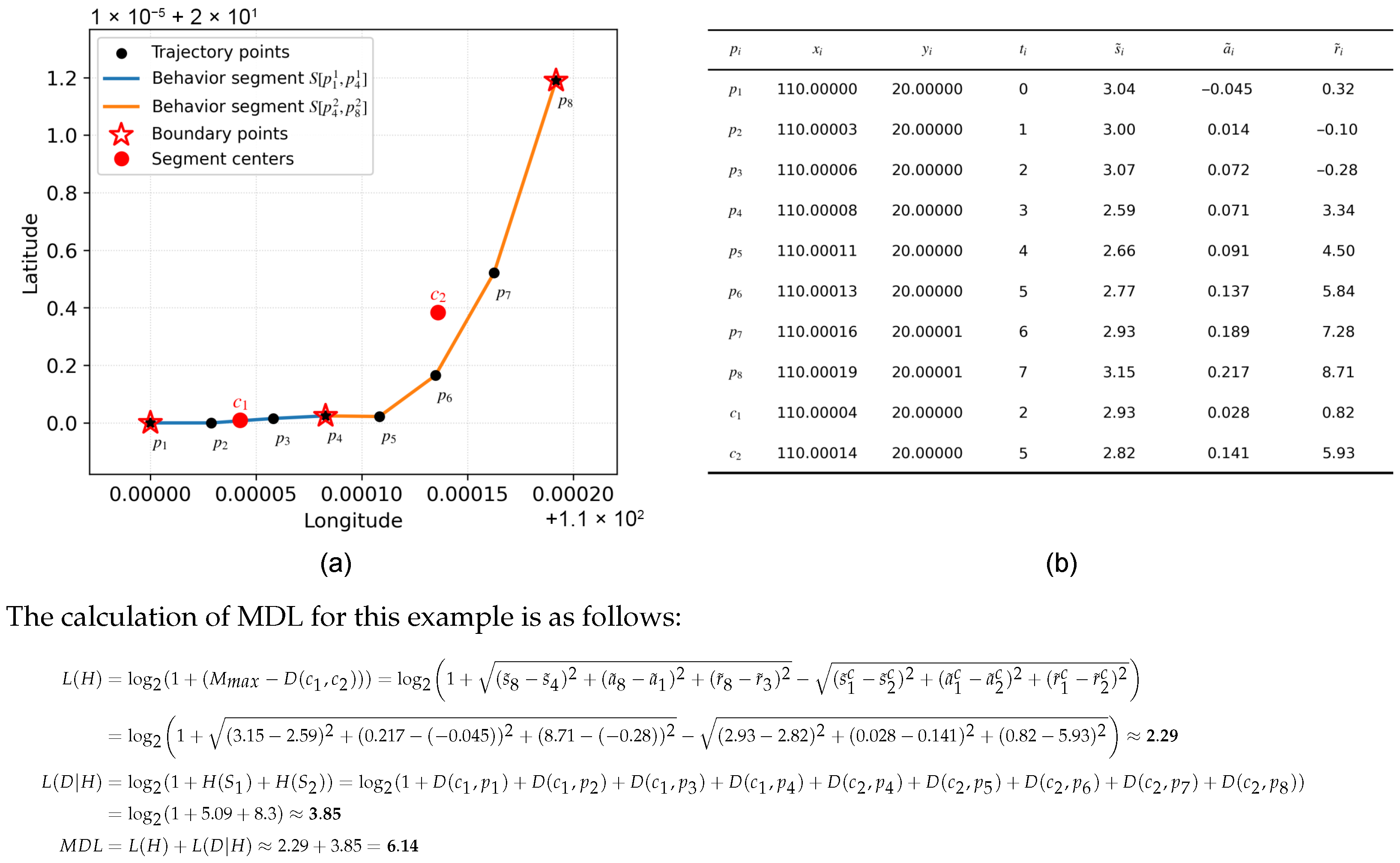
Figure 4 shows an example of trajectory segmentation and MDL cost formulation using a sample trajectory consisting of eight points, where each point is characterized by three movement features, including speed, acceleration, and turning rate. According to the trajectory segmentation problem, candidate points are evaluated to determine boundary points. In this example, point $p_4\in C_p$ is selected as the segment boundary. Together with the start and end points, the trajectory is divided into two behavior segments, $S[p_1^1,p_4^1]$ and $S[p_4^2,p_8^2]$. For each segment, a representative centroid $(c_1,c_2)$ is calculated based on the mean values of the three features. The details of all points are summarized in the Trajectory Information Table.

The MDL cost is then computed based on Equation (10). The maximum dissimilarity term $M_{max}$ is defined by the extreme feature differences observed in the trajectory, including the maximum and minimum values of speed $({\tilde{s}}_8,{\tilde{s}}_4)$, acceleration $({\tilde{a}}_8,{\tilde{a}}_1)$, and turning rate $({\tilde{r}}_8,{\tilde{r}}_3)$. This normalization ensures that the model description length reflects relative behavioral variations within the trajectory. The proposed method of segmentation and optimization is detailed in Section 3.5.

3.5. Matheuristic Fixed Set Search

The Fixed Set Search (FSS) [54] is a learning-based metaheuristic that exploits common elements among high-quality solutions to guide the search process in combinatorial optimization problems. The Matheuristic Fixed Set Search (MFSS) [55] extends this concept into a matheuristic framework by embedding a mixed-integer programming (MIP) solver within the local search phase. The MFSS framework consists of several key components, including the reformulation of the original problem for algorithmic encoding and solver integration, the initialization of high-quality solutions to enhance the quality of the initial fixed set, the generation of fixed sets based on common elements extracted from encoded solutions, and the improvement of population quality to strengthen the fixed set and promote convergence toward globally optimal solutions.

3.5.1. Problem Reformulation

In trajectory segmentation, the elements shared among solutions correspond to segments rather than individual boundary points. Because each segment is determined by both its start and end boundaries, any change to either will create a new segment. Therefore, it is necessary to reformulate the problem from point-based to segment-based selection. To facilitate the integration of the optimization process with the MDL-based cost and to support a direct implementation of fixed set constraints and MIP, this framework reformulates the decision variable from a pointwise binary vector $x_i$ to a segment-based binary matrix $x_{ij}$. This transformation replaces nonlinear dependencies on segment boundaries with linear combinations of precomputed constants. As a result, segment-level availability and fixed set constraints can be incorporated directly into the optimization framework.

In this revised formulation, two binary decision variables are introduced. The first, $x_{ij}$, indicates whether the segment $S[p_i^k,p_j^k]$ is selected. The second, $y_{izj}$, identifies pairs of consecutive segments $S[p_i^k,p_z^k]$ and $S[p_z^{k+1},p_j^{k+1}]$, capturing inter-segment relationships. The candidate-set constraint (11) from the pointwise model is reformulated as an availability matrix $A_{ij}$, where $A_{ij}=1$ only if both endpoints $p_i$ and $p_j$ are candidates. Within the MDL model, the inter-segment centroid distance term $D(c_k,c_{k+1})$ is replaced by a precomputed matrix $D_{izj}$ with distance between any pair of centroids of segments $S[p_i^k,p_z^k]$ and $S[p_z^{k+1},p_j^{k+1}]$, and the within-segment description term $H\left(S_k\right)$ is replaced by a standard deviation matrix $H_{ij}$, where $i,z,j$ correspond to segment boundaries.

$$\begin{array}{cc}\hfill \underset{x,y}{min}& {log}_2\left(1+\sum _{i=1}^{n-2}\sum _{z=i+1}^{n-1}\sum _{j=z+1}^n\left(M_{max}-D_{izj}{y}_{izj}\right)\right)+{log}_2\left(1+\sum _{i=1}^{n-1}\sum _{j=i+1}^n{H}_{ij}{x}_{ij}\right)\hfill \end{array}$$

(14)

$$\begin{array}{cc}\hfill \mathrm{s}.\mathrm{t}.& x_{ij}\le A_{ij},\forall 1\le i<j\le n,\hfill \end{array}$$

(15)

$$\begin{array}{cc}\hfill & \sum _{j=2}^n{x}_{1j}=1,\sum _{i=1}^{n-1}{x}_{in}=1,\hfill \end{array}$$

(16)

$$\begin{array}{cc}\hfill & \sum _{i=1}^{z-1}{x}_{iz}=\sum _{j=z+1}^n{x}_{zj},\forall 1\le i<z<j\le n,\hfill \end{array}$$

(17)

$$\begin{array}{cc}\hfill & x_{ij}=1,\forall S[p_i^k,p_j^k]\in F,\hfill \end{array}$$

(18)

$$\begin{array}{cc}\hfill & y_{izj}\le x_{iz},y_{izj}\le x_{zj},y_{izj}\ge x_{iz}+x_{zj}-1,\forall 1\le i<z<j\le n,\hfill \end{array}$$

(19)

$$\begin{array}{cc}\hfill & x_{ij}\in \{0,1\},y_{izj}\in \{0,1\},\forall \mathrm{valid}(i,j),(i,z,j).\hfill \end{array}$$

(20)

Constraint (15) enforces candidate availability, while constraints (16) ensure unique start and end segments, analogous to the original formulation. Constraint (17) guarantees segment continuity at intermediate points by enforcing flow conservation. Constraint (18) fixes segments that belong to the pre-defined fixed set F. Constraint (19) linearize the inter-segment selection, ensuring $y_{ijk}=1$ if and only if both corresponding segments are selected, so that $D_{ijk}$ contributes linearly to the objective.

3.5.2. Solution Initialization

A desirable solution population $Ln$ is essential for MFSS. The fixed set is built from elements that recur in high-quality solutions; therefore, both solution quality and solution diversity are critical to the effectiveness of the fixed set. Standard segmentation methods (e.g., sliding window, top-down) are often deterministic and yield a single solution for a given parameter choice, which limits diversity. To produce a pool of distinct high-quality solutions during initialization, this step combines the top-down strategy with a Greedy Randomized Adaptive Search construction, referred to as the Greedy Randomized Top-Down (GRTD) algorithm. GRTD follows a top-down recursive process, in which controlled randomness is introduced in the selection of split points at each recursion, allowing the initialization to produce a variety of competitive segmentation solutions.

In the GRTD algorithm, the Greedy Randomized Construction (GRC) introduces stochasticity by generating a Restricted Candidate List (RCL) of split points within the current segment. The RCL is constructed by selecting the top $\kappa$ split points with the lowest segmentation costs, thus balancing quality and diversity in the generated population. A smaller $\kappa$ prioritizes optimal splits to ensure high-quality individual solutions but may lead to a homogeneous population (intensification), whereas a larger $\kappa$ increases the probability of selecting points of lower quality to enhance diversity (diversification). The top-down procedure then recursively partitions a segment by randomly selecting a split point from the RCL, producing multiple competitive yet distinct candidate solutions for subsequent fixed set extraction. To ensure computational efficiency and prevent unproductive recursion, a fail limit parameter L is introduced. This mechanism acts as a termination criterion, halting the recursive process when consecutive split attempts fail to yield an improvement, thereby avoiding infinite loops and stagnation. The initialization process is outlined in Algorithm 1.

Algorithm 1 GRTD: Greedy Randomized Top-Down Initialization.

1: Input: Trajectory point set P, candidate point set $C_p$, availability matrix A, variance matrices $D,H$  2: Parameters: RCL size $\kappa$, fail limit L, population size $\tilde{n}$  3: Output: Solution population $Ln$ of segmentation matrices X  4: function Init($P,C_p,A,D,H$)  5:        $Ln\leftarrow ⌀$,$\mathrm{fail}\mathrm{count}c=0$  6:        for $r=1$ to $\tilde{n}$ do  7:             $\mathrm{sol}\leftarrow \{0,n-1\}$  8:             Split($0,n-1,\mathrm{sol},c$)                                                                                 ▹ See function defined below  9:             Convert sorted sol to binary matrix X and add X to $Ln$ 10:        end for 11:        return $Ln$ 12: end function 13: function Split($i,j,\mathrm{sol},c$) 14:        if $j\le i+1$ or $c\ge L$ then return 15:        end if 16:        $\mathrm{Candidates}\mathrm{set}Z\leftarrow \{z\mid i<z<j,p_z\in C_p,A_{iz}=A_{zj}=1\}$ 17:        if $Z=⌀$ then return 18:        end if 19:        for $z\in Z$ do compute $\Delta \mathrm{Cost}(i,z,j)$ using Equation (21) 20:        end for 21:        Sort Z by $\Delta \mathrm{Cost}(i,z,j)$; define RCL as first $min(\kappa ,|Z\left|\right)$ 22:        Randomly select $z^{\ast }$ from RCL 23:        if $\Delta \mathrm{Cost}(i,z^{\ast },j)<0$ then $c\leftarrow 0$ 24:        else   $c\leftarrow c+1$ 25:        end if 26:        if $c>L$ then return 27:        end if 28:        Insert $p_{z^{\ast }}$ into sol 29:        Split($i,z^{\ast },\mathrm{sol},c$); Split($z^{\ast },j,\mathrm{sol},c$) 30: end function

The way to determine RCL with relatively low segmentation costs is to capture the difference in MDL costs before and after segmentation. Consider a current interval $S[p_i^k,p_j^k]$ with neighboring previous segment $S[p_u^{k-1},p_i^{k-1}]$ and next segment $S[p_j^{k+1},p_v^{k+1}]$. Split candidates $p_z$ (with $i<z<j$ and $p_z\in C_p$) are evaluated by the change in the MDL cost induced by splitting $S_k$ at $p_z$ with two new segments, $S[p_i^{k^1},p_z^{k^1}]$ and $S[p_z^{k^2},p_j^{k^2}]$. The cost difference $\Delta \mathrm{Cost}(i,z,j)$ introduced by this split, is computed based on the original local cost $C_{\mathrm{orig}}$ and the cost after the split $C_{\mathrm{split}}$, which are defined as follows.

$$\begin{array}{cc}\hfill & \Delta \mathrm{Cost}(i,z,j)={\mathrm{C}}_{\mathrm{split}}-{\mathrm{C}}_{\mathrm{orig}}\hfill \\ \hfill & {\mathrm{C}}_{\mathrm{orig}}={log}_2\left(1+\left(M_{max}-D_{uij}\right)+\left(M_{max}-D_{ijv}\right)\right)+{log}_2\left(1+H_{ij}\right)\hfill \\ \hfill & {\mathrm{C}}_{\mathrm{split}}={log}_2\left(1+\left(M_{max}-D_{uiz}\right)+\left(M_{max}-D_{izj}\right)+\left(M_{max}-D_{zjv}\right)\right)+{log}_2\left(1+H_{iz}+H_{zj}\right)\hfill \end{array}$$

(21)

3.5.3. Fixed Set Generation

The procedure for generating a fixed set of segments, denoted as F with a controllable size (cardinality) $\left|F\right|$, is now described. This set is intended to produce feasible solutions of equal or superior quality compared to those previously generated. The following definitions are introduced: $Ln$ represents the list of $\tilde{n}$ best solutions in the population, which constitutes the segment set $Ln={\widehat{S}}_1,..,{\widehat{S}}_n$, produced during the segment building process in the initialization or earlier steps of the MIP solver in the algorithm. A base solution $Bs\in Ln$ is a solution chosen randomly from the n best solutions. If a fixed set satisfies $F\subset Bs$, it can be utilized to generate a feasible solution of at least the same quality as $Bs$, with F having the freedom to include any number of segments of $Bs$. The primary goal is to construct F such that it includes frequently occurring segments in a group of high-quality solutions. $Ls$ is a subset of $\tilde{m}$ randomly chosen solutions from $Ln$, $\tilde{m}<\tilde{n}$. To identify common segments between the base solution $Bs$ and the selected solution set $Ls$, the function $C(S_t^{Bs},{\widehat{S}}_k^{Ls})$ is introduced. Here, $S_t^{Bs}$ denotes the $t^{th}$ segment in the base solution $Bs$, where $t=1,\dots ,\mid {\widehat{S}}_{Bs}\mid$, and ${\widehat{S}}_k^{Ls}$ denotes the $k^{th}$ segment set within the chosen solution set $Ls$. The function $C(S_t^{Bs},{\widehat{S}}_k^{Ls})$ outputs 1 if $S_t^{Bs}$ is present in ${\widehat{S}}_k^{Ls}$, and 0 otherwise. Utilizing this function, the frequency of each segment in the base solution $Bs$ across all segment sets of the selected solution set $Ls$ can be determined. These frequencies are stored in the set $CO$, where each element $C{O}_t$ comprises the segment $S_t^{Bs}$ and its occurrence count $O(S_t^{Bs},Ls)$.

$$O(S_t^{Bs},Ls)=\sum _{k=1}^{\tilde{m}}C(S_t^{Bs},{\widehat{S}}_k^{Ls})(t=1,\dots ,\mid {\widehat{S}}_{Bs}\mid )$$

(22)

The fixed set $F\subset Bs$ is defined to include segments $S_t^{Bs}$ that have a relatively high occurrence frequency, indicated by the function $O(S_t^{Bs},Ls)$. This function measures how frequently each segment from the base solution $Bs$ appears within the selected solution set $Ls$. Given that the quality of both the base solution $Bs$ and the chosen solution set $Ls$ can vary due to their random selection, flexibility is incorporated in determining the size of the fixed set. Rather than specifying its size exactly, an adaptive mechanism is employed in which the fixed set size is initialized as $f_{init}$ and subsequently reduced by a factor of $R_f$ when no improved solution is found after a series of attempts. This flexible adjustment enhances the search process by dynamically expanding the solution space as needed, and also helps to ensure that the fixed set consistently maintains a high quality.

3.5.4. Population Evolution

The population is updated by replacing the worst solution with any newly discovered feasible solution of superior quality, thus maintaining a constant population size while enhancing overall quality. This replacement mechanism ensures efficient population improvement with stable computational cost. New solutions are generated through a balance of exploration and exploitation. Exploration increases diversity by searching new areas using various fixed sets, while exploitation focuses on improving current promising solutions via local search with the MIP solver. Details of these mechanisms in MFSS are provided below.

Exploration is maintained through two adaptive mechanisms. First, by randomly selecting a subset $Ls$ from the top $\tilde{n}$ solutions, overlap among chosen solutions remains low, resulting in more diverse fixed sets F. Second, the algorithm adaptively changes the fixed set ratio. When no improvement is observed for several iterations, the ratio is decreased to expand the search space and enhance exploration.

Exploitation is achieved through an MIP-based local search that improves individual solutions in the population. Each candidate solution is re-optimized using a reformulated mathematical model with fixed set constraint, using the base solution $Bs$ as a hot start for the MIP solver. This approach narrows the search space and significantly reduces the computation time. If no better solution is found after several iterations, the time limit of the solver is increased to explore a larger neighborhood and help escape local optima.

These approaches combine exact optimization with heuristic refinement to intensify the search near promising solutions, while structural variation promotes exploration of new regions. An adaptive balance between diversification and intensification preserves population diversity as it evolves toward possibly optimal regions.

The overall procedure of the MFSS algorithm is summarized in Algorithm 2.

Algorithm 2 MFSS: Matheuristic Fixed Set Search.

1: Input: Trajectory point set P, candidate point set $C_p$, availability matrix A, variance matrices $D,H$  2: Parameters: population size $\tilde{n}$, population subset size $\tilde{m}$, max stagnation $sta{g}_{max}$, fixed set size $f_{init}$ and rate $R_f$, IP initial solving time ${\tau }_{init}$ and rate $R_{\tau }$, max time limit $TL$ for the MIP solver, stall limit $SL$  3: Output: Best-found segmentation ${\widehat{S}}_{best}$  4: function MFSS($P,C_p,A,D,H$)  5:     $f\leftarrow f_{init}$, $\tau \leftarrow {\tau }_{init}$, $stag\leftarrow 0$, $stall\leftarrow 0$  6:     $Ln\leftarrow$Init($P,C_p,A,D,H$)                                                                               ▹ See Algorithm 1  7:     sort $Ln$ ascending by $MDL\left({\widehat{S}}_k\right)$ in Equation (14); ${\widehat{S}}_{best}\leftarrow$ first($Ln$)  8:     while $\tau <TL$ and $stall<SL$ do  9:           $F\leftarrow$Fix($Ln,\tilde{m},f$)                                                                               ▹ See function defined below 10:          $Ln\leftarrow Ln\cup$IPS($F,\tau$)                                                                               ▹ MIP-based solver 11:          sort $Ln$ ascending by $MDL\left({\widehat{S}}_k\right)$; remove worst; $\widehat{S}\leftarrow$ first($Ln$) 12:          if $MDL\left(\widehat{S}\right)<MDL\left({\widehat{S}}_{best}\right)$ then 13:                ${\widehat{S}}_{best}\leftarrow \widehat{S}$; $stag\leftarrow 0$, $stall\leftarrow 0$ 14:          else 15:                $stag\leftarrow stag+1$, $stall\leftarrow stall+1$ 16:          end if 17:          if $stag\ge sta{g}_{max}$ then 18:                $stag\leftarrow 0$; $\tau \leftarrow \tau R_{\tau }$; $f\leftarrow f{R}_f$ 19:          end if 20:     end while 21:     return ${\widehat{S}}_{best}$ 22: end function 23: function Fix($Ln,\tilde{m},f$) 24:     select random $Bs\in Ln$; generate random $Ls\in Ln$ of size $\tilde{m}$ 25:     $CO\leftarrow CO\cup \{S_t^{Bs},O(S_t^{Bs},Ls)\}$ 26:     sort $CO$ descending by $O(S_t^{Bs},Ls)$ 27:     $F\leftarrow$ top $f^{th}$ segments in $CO$ 28:     return F 29: end function

4. Experiment and Results Analysis

4.1. Data Source

To validate the effectiveness of the proposed methods, a case study was conducted in the Qiongzhou Strait, located between the Leizhou Peninsula and Hainan Island in southern China. The Qiongzhou Strait serves as a critical maritime corridor connecting the South China Sea and Beibu Gulf. This area is characterized by intensive east–west commercial traffic, frequent north–south ferry and fishing activities, and has complex navigation controls under the mandatory traffic separation scheme.

In this study, the center of the strait was selected as the experimental area, defined by a rectangular region extending from 109°52′19″ E to 110°25′13″ E and 19°55′32″ N to 20°17′51″ N. This area represents the busiest and most behaviorally diverse zone of maritime traffic within the strait, where vessel behaviors are subject to strict navigation regulations and heterogeneous operational patterns. This region also includes Xuwen Port, which is the largest roll-on/roll-off passenger and cargo port globally. Intensive north-south traffic associated with this port alters vessel movement patterns in the east-west main channel and increases the operational complexity of the area.

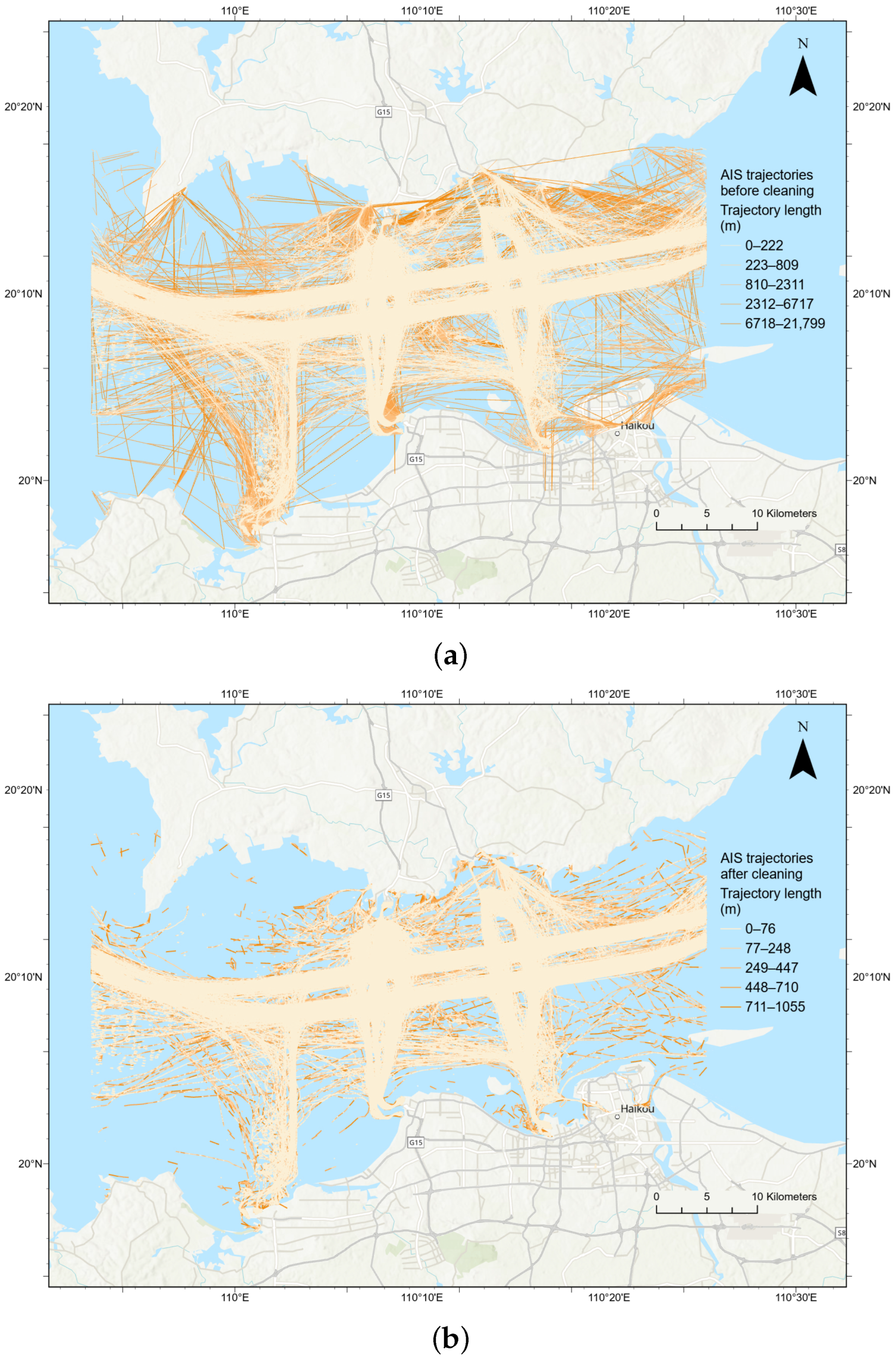
The AIS trajectory data were acquired from HiFleet2, a leading maritime data provider. This dataset aggregates signals from a network of terrestrial base stations and satellite receivers to ensure high coverage and reliability in the study area. The data used in this study cover the period from 25 August to 31 August 2025, comprising 3,123,262 trajectory points from 2414 vessels of 22 different types. A general overview of the study area and spatial distribution of the original trajectories is provided in Figure 5. Since AIS data were collected in both static and dynamic forms, the corresponding fields used in this study are summarized in Appendix A (

Table A1. Sample of original AIS trajectory data used in this study.

Static Information					Dynamic Information
MMSI	Ship Type	W (m)	L (m)		Lon	Lat	Spd (kn)	Hdg (°)	Crs (°)	Nav. Status *	Timestamp
413508170	Chemical/Oil tanker	14	89		110.23489	20.16195	7.3	78	76.6	UWE	2025/08/31 00:00:08
413210640	Container ship	24	129		110.26017	20.06549	7.0	302	341.1	UWE	2025/08/31 00:00:08
413232470	Passenger ship	21	128		110.13545	20.22967	3.3	61	50.3	UWE	2025/08/31 00:00:08
412522250	Ro-Ro passenger ship	22	165		110.11448	20.21002	11.3	16	17.4	UWE	2025/08/31 00:00:08
413358570	Bulk carrier	16	99		110.15248	20.17945	10.4	511	263.3	UWE	2025/08/31 00:00:08
413523230	Passenger ship	20	123		110.13617	20.23290	0.0	0	21.8	MRD	2025/08/31 00:00:08
412000002	Fishing vessel	5	20		110.23166	20.27136	5.8	511	111.0	UNK	2025/08/31 00:00:08

* Abbreviations of navigation status: UWE—Under way using engine; MRD—Moored; UNK—Unknown.

), which presents the original decoded data attributes.

4.2. Baselines and Experimental Setup

Classical Sliding Window segmentation (SWS) and Top-Down segmentation (TDS) are adopted as baselines to evaluate segmentation performance [26]. To ensure a fair comparison, adaptive versions of SWS and TDS were implemented to segment trajectories by comparing the same dissimilarity measure $D(p_i,p_j)$ in Equation (1) with an adaptive threshold that is iteratively tuned until the number of behavioral segments equals that of MFSS. This design minimizes the potential bias caused by dissimilarity calculation and differences in segment count, allowing a more reasonable comparison of behavioral consistency among different methods.

The behavioral classes were derived from the point labels generated by the Jenks algorithm for the movement features during the decomposition (see Section 3.3) and were used for the evaluation of the results. The key feature points derived from these label transitions were also aggregated as the Jenks-based segmentation result for comparison. In addition, these labels were used as a reference to analyze the behavioral interpretability of MFSS, SWS, and TDS, which do not inherently provide labels. For each segment $S_k$, the behavioral class $L_c^{S_k}$ of a movement feature was assigned according to the labels that occurred most frequently among the points within that segment.

The original trajectory data were preprocessed by removing records with missing attributes, duplicate points, and extreme outliers to ensure data quality. Preprocessed trajectories with fewer than 30 records were excluded to avoid behavioral instability. All segmentation algorithms were implemented in C++ and compiled with the C++20 standard. Experiments were conducted on a computer equipped with an Intel Core i9-14900KF CPU and 32 GB RAM. Subproblems in the MFSS procedure were solved using ILOG CPLEX 22.1.1. Visualizations and plots were generated using Python 3.13 and ArcGIS Pro 3.5.0. Detailed parameter configurations for the proposed MFSS algorithm can be found in Appendix B (

Table A2. Parameter settings used in the MFSS algorithm.

Parameter	Description	Value
$\tilde{n}$	Population size (number of solutions maintained in the pool)	20
$\tilde{m}$	Size of randomly chosen subset for similarity evaluation	8
$sta{g}_{max}$	Maximum number of stagnation iterations before parameter update	10
$f_{init}$	Initial size of fixed segment set (adaptive to m)	$0.7m$
$R_f$	Adjustment rate of fixed set size when stagnation occurs	0.95
${\tau }_{init}$	Initial time limit (s) for the MIP solver (adaptive to n)	$0.005n$
$R_{\tau }$	Adjustment rate of MIP solver time limit during search	1.2
$TL$	Overall runtime limit of the MFSS process (adaptive to n)	$0.1n$
$SL$	Stall limit: maximum consecutive iterations without improvement	50

).

4.3. Evaluation Metrics

The segmentation performance is evaluated using seven indicators: Davies–Bouldin Index, Silhouette Coefficient, Calinski–Harabasz Index, Average Intra-Segment Variance, Average Inter-Segment Variance, Average Purity, and Average Coverage. These metrics jointly assess the consistency, compactness, and distinctiveness of behavioral segments derived from the trajectory point set P, while the two variance metrics reflect the MDL balance between minimum distortion and maximum compression.

Definition 5

(Davies–Bouldin Index (DBI)). DBI evaluates the trade-off between segment compactness and separation:

$$\mathrm{DBI}={\displaystyle \frac{1}{m}}\sum _{i=1}^m\underset{j\ne i}{max}{\displaystyle \frac{{\sigma }_i+{\sigma }_j}{D(c_i,c_j)}}$$

(23)

where $D(·,·)$ is the behavioral dissimilarity defined in Equation (1), and ${\sigma }_k={\displaystyle \frac{1}{|S_k|}}{\sum }_{p_i\in S_k}D(p_i,c_k)$. Lower values indicate tighter and more distinctive clusters.

Definition 6

(Silhouette Coefficient (SC)). For each point $p_i$, let $a_i$ be the mean intra-segment distance and $b_i$ the smallest mean distance to another segment. A higher SC indicates more cohesive and well-separated segments.

$$s_i={\displaystyle \frac{b_i-a_i}{max(a_i,b_i)}}\mathrm{SC}={\displaystyle \frac{1}{n}}\sum _{i=1}^n{s}_i$$

(24)

Definition 7

(Calinski–Harabasz Index (CHI)). CHI measures the ratio of between-segment to within-segment dispersion:

$$\mathrm{CHI}={\displaystyle \frac{\mathrm{tr}\left(B_m\right)/(m-1)}{\mathrm{tr}\left(W_m\right)/(n-m)}}$$

(25)

where $\mathrm{tr}\left(B_m\right)$ and $\mathrm{tr}\left(W_m\right)$ denote the trace of between-segment and within-segment scatter matrices. Higher CHI values indicate clearer separation boundaries.

Definition 8

(Average Intra-Segment Variance (ISV)). ISV quantifies the average internal dispersion using the cohesiveness measure $H\left(S_k\right)$ defined in Equation (2). Smaller ISV values represent stronger behavioral uniformity within segments.

Definition 9

(Average Inter-Segment Variance (ESV)). ESV quantifies the average behavioral dissimilarity between adjacent segment centroids, consistent with the transition term $D(c_k,c_{k+1})$ defined in Equation (3). It reflects the degree of behavioral distinction across consecutive segments, where a higher ESV indicates clearer differentiation of motion patterns along the trajectory.

Definition 10

(Average Purity (AP)). Purity measures the internal consistency between the generated segments and the reference behavioral classes obtained from Jenks clustering across all feature domains. Let $L_c^{S_k}$ be the behavioral class of segment $S_k$ and $L_c^{p_i}$ the Jenks-based label of point $p_i$, which belongs to the set of all possible labels $\mathcal{C}$. For each segment $S_k$, its behavioral class $L_c^{S_k}$ is determined by the majority labels among all points within the segment, as defined below:

$$L_c^{S_k}=arg\underset{c\in \mathcal{C}}{max}\left|\{p_i\in S_k\mid L_c^{p_i}=c\}\right|$$

(26)

The purity of a segment $S_k$ is then given by the proportion of points whose labels match its assigned behavioral class. The final AP is obtained by averaging the segment-level purities over all segments.

$$\mathrm{AP}={\displaystyle \frac{1}{m}}\sum _{S_k\in \widehat{S}}{\displaystyle \frac{\left|\right\{p_i\in S_k\mid L_c^{p_i}=L_c^{S_k}\left\}\right|}{|S_k|}}$$

(27)

Definition 11

(Average Coverage (AC)). Coverage quantifies how well the predicted segments overlap with the Jenks-derived reference segments $\mathcal{G}=\{G_1,\dots ,G_M\}$, which are obtained by splitting the trajectory whenever a point label changes in any of the three feature domains. For each $G_i$, the coverage ratio is calculated as follows. A higher AC value indicates a greater overlap between predicted and reference segments.

$$\mathrm{AC}\left(G_i\right)=\underset{S_k\in \widehat{S}}{max}{\displaystyle \frac{|G_i\cap S_k|}{|G_i|}},\mathrm{AC}={\displaystyle \frac{1}{M}}\sum _{i=1}^M\mathrm{AC}\left(G_i\right).$$

(28)

4.4. Data Preprocessing Results

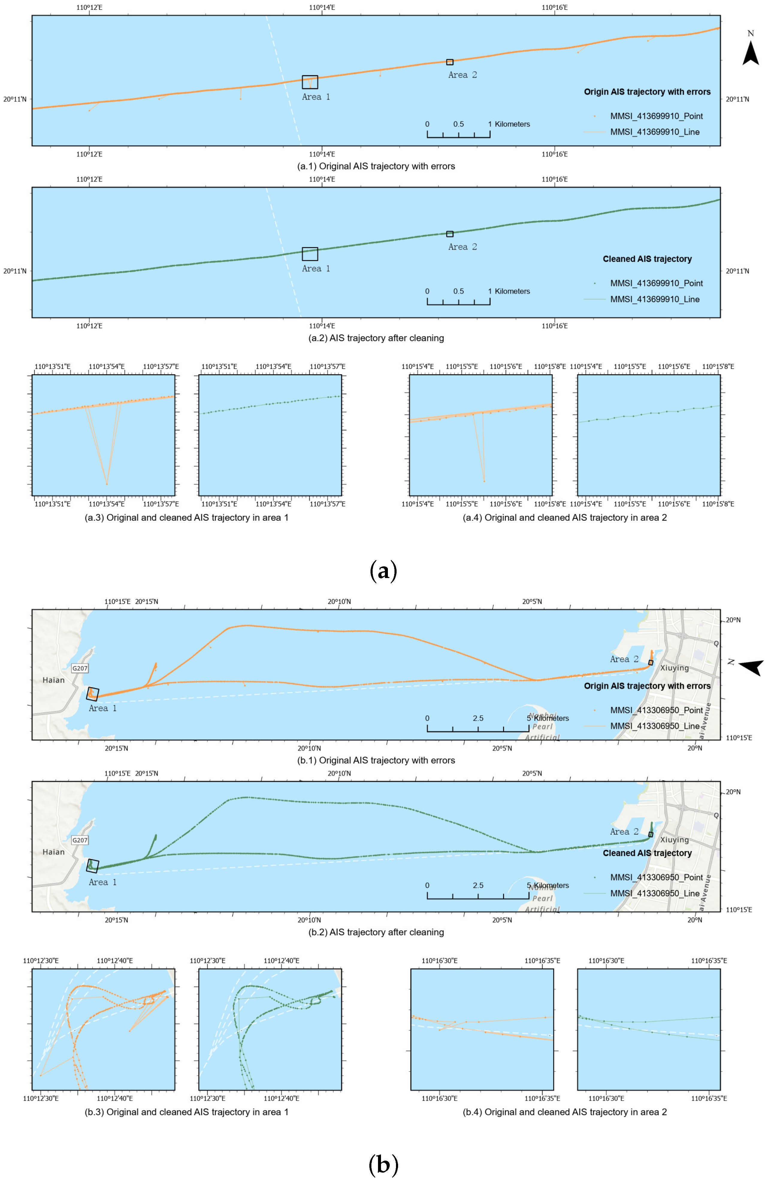
Preprocessing is a prerequisite for reliable behavioral segmentation. We first evaluate the effectiveness of our cleaning framework on the entire dataset. Figure 6 compares the original AIS trajectories with the cleaned dataset. The original data in Figure 6a contains significant noise and missing values. Coastal areas specifically exhibit frequent position jumps that generate spurious trajectory segments and erroneous points located on land. Furthermore, prolonged signal interruptions in these regions often result in unrealistic long straight segments that violate normal navigation patterns. To address these issues, we implemented a sequential preprocessing strategy. To handle missing points, trajectories containing time gaps exceeding 20 min were divided into independent sub-trajectories to mitigate the artifacts of data loss. Subsequently, spatial and temporal anomalies were identified and removed from these sub-trajectories. Following this process, the cleaned trajectories in Figure 6b clearly delineate the main shipping routes. Finally, approximately 20% of the original data points were identified as anomalies and removed.

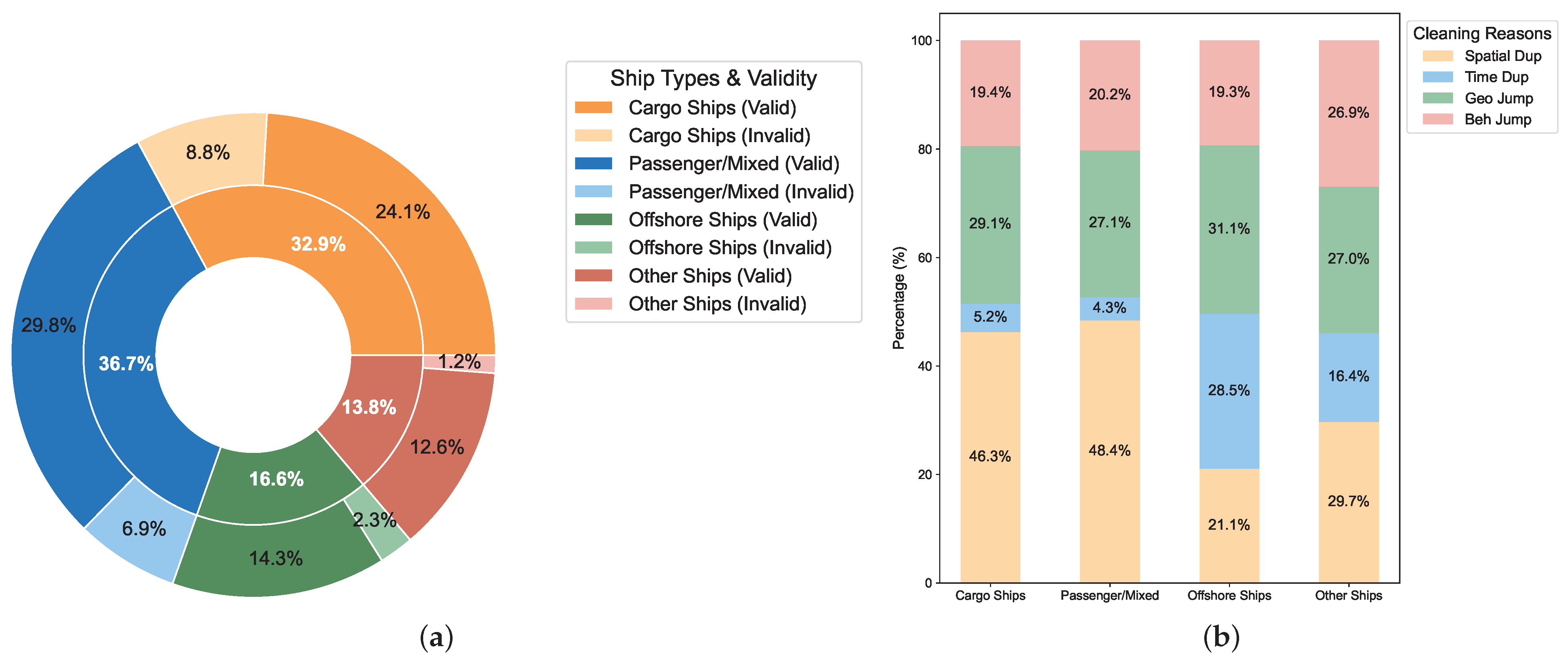
To provide deeper insight into data quality, Figure 7 presents the validity ratio and error distribution across four vessel categories, including Cargo, Passenger, Offshore, and Others. North-south bound passenger ships and east-west bound cargo ships dominate the traffic volume with shares of 36.7% and 32.9%, respectively. These two categories also exhibit substantial error rates of 18.8% and 26.75%. Figure 7b further decomposes the removed data into specific error categories.

As indicated in Figure 7b, data redundancy constitutes a prevalent issue. We address this by differentiating between spatial and temporal duplicates as detailed in

Table 1. Examples of data cleaning for duplicate records with spatial and temporal conflicts. The underlined rows represent erroneous data removed during preprocessing.

Lon (°)	Lat (°)	Speed (kn)	Course (°)	Heading (°)	Time
(a) Duplicate Records (MMSI: 100661111): Identical information repeated at adjacent timestamps
110.06675	20.12604	6.8	68.0	68.4	2025/8/31 02:12:17
110.07040	20.12759	3.4	68.0	68.3	2025/8/31 02:14:26
110.07040	20.12759	3.4	68.0	68.3	2025/8/31 02:14:27
110.07040	20.12759	3.4	68.0	68.3	2025/8/31 02:14:29
110.07394	20.12876	3.2	78.0	78.4	2025/8/31 02:16:38
(b) Temporal Conflicts (MMSI: 101103668): Multiple distinct points recorded at the exact same timestamp
110.04914	20.13507	3.7	74.0	74.9	2025/8/30 23:36:02
110.04957	20.13517	3.8	74.0	74.6	2025/8/30 23:37:02
110.05036	20.13534	3.7	78.0	78.5	2025/8/30 23:37:02
110.04986	20.13523	3.7	78.0	78.0	2025/8/30 23:37:02
110.04970	20.13520	3.7	78.0	78.4	2025/8/30 23:37:02
110.05103	20.13555	3.8	77.0	77.6	2025/8/30 23:38:02

. For spatial duplicates characterized by identical location and kinematic information at adjacent timestamps, the system retains only the initial valid entry to eliminate redundancy. In cases of temporal duplicates where conflicting points share a single timestamp, validity is determined by assessing spatial continuity. The point minimizing the SED relative to its neighbors is preserved to ensure kinematic consistency.

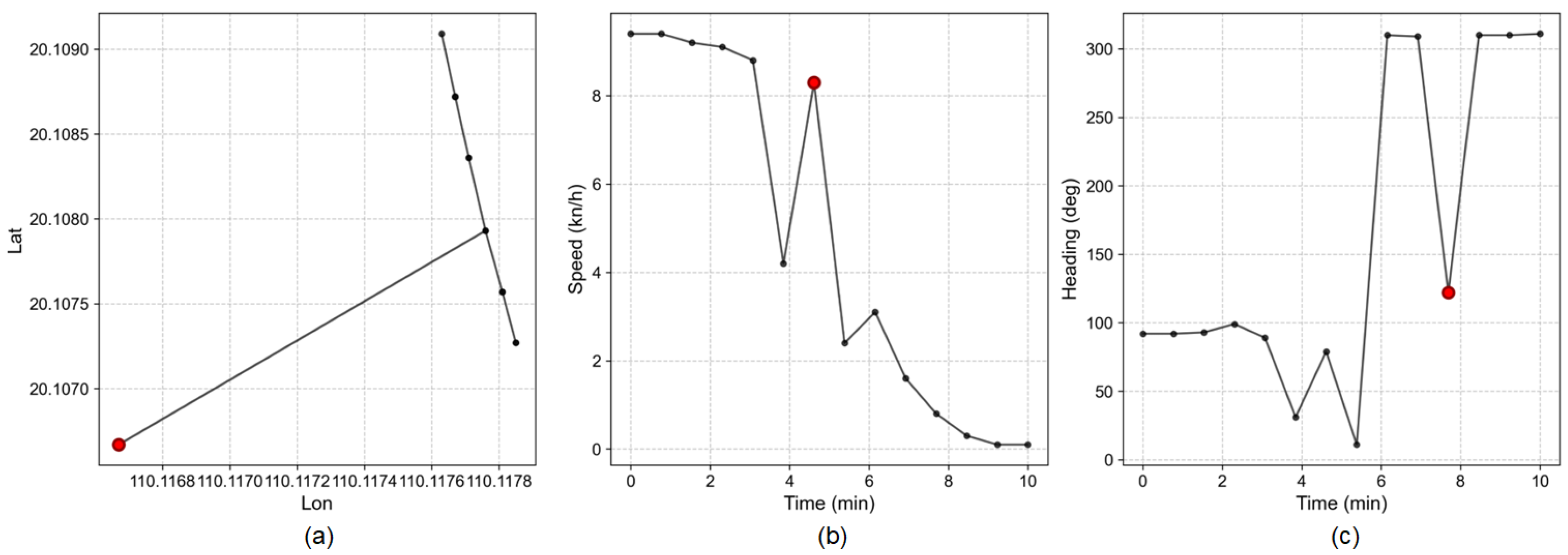
Beyond redundancy, the dataset highlights significant geographic and behavioral anomalies such as drift and speed mismatches. These anomalies manifest as unrealistic jumps in the trajectory. We implement the sliding window detection mechanism described in Section 3.2 to identify these abrupt transitions. Figure 8 visualizes typical outliers where the proposed algorithm effectively distinguishes and filters out spatial jumps and unrealistic kinematic spikes while maintaining the overall motion trend.

The effectiveness of this comprehensive cleaning framework on individual trajectories is demonstrated in Figure 9. For MMSI 413699910 representing typical East-West traffic, the algorithm successfully resolves significant position jumps and redundant data clusters observed in Area 1 and Area 2. Similarly, for the North-South trajectory of MMSI 413306950, errors resulting from precision loss in port waters are effectively corrected.

4.5. Segmentation Results

Based on the high-quality trajectory dataset obtained from the preprocessing stage described in Section 4.4, we conducted a comprehensive evaluation of the proposed MFSS framework. This section presents the experimental results in three dimensions. We perform a quantitative analysis to assess segmentation quality using evaluation metrics in Section 4.3. Then, trajectory movement patterns are visualized to validate the method’s capability in capturing spatial distributions of speed, acceleration, and turning patterns. Finally, we analyze derived trajectory segment behaviors through a case study in Xuwen Port to demonstrate the semantic coherence and interpretability of the generated segments compared to baseline methods.

4.5.1. Evaluation Analysis

Table 2. Comparison of segmentation performance among MFSS, SWS, TDS, and Jenks using the one-week cleaned AIS dataset. The best performance for each metric is highlighted in bold.

Method	DBI	SC	CHI	ISV	ESV	AP (%)	AC (%)
MFSS	1.685	0.120	12.031	0.274	0.786	70.547	98.881
SWS	2.578	0.085	6.335	0.355	0.673	70.615	98.915
TDS	1.973	0.064	4.911	0.370	0.767	70.287	99.163
Jenks	7.340	−0.414	1.938	0.213	0.251	80.865	86.353

illustrates the segmentation performance of MFSS and the baselines (SWS, TDS, Jenks) across the evaluation metrics. Overall, MFSS yields a well-balanced result, outperforming the baselines on standard clustering metrics and on MDL-related variance measures, while remaining competitive on purity and coverage. In other words, MFSS improves segment compactness and separability without degrading alignment to the Jenks-derived labels.

An examination of Table 2 reveals that MFSS produces more compact and better-separated segments compared to the baseline approaches. This is evidenced by its markedly lower DBI, larger SC, and higher CHI, suggesting that the segments identified by MFSS are internally more homogeneous and distinct from one another. Specifically, MFSS achieves a DBI that is 34.6% and 14.6% lower than that of SWS and TDS, respectively. Similarly, MFSS attains a CHI that is 89.9% and 145% higher compared to SWS and TDS. Although SC values remain relatively low due to the interaction among multiple features, MFSS still outperforms SWS and TDS by 41.2% and 87.5% in this metric, respectively. These improvements are attributed to the segment-level optimization strategy of MFSS, which evaluates candidate boundaries jointly with neighboring intervals to reliably detect meaningful behavioral transitions and suppress over-segmentation caused by transient fluctuations.

Regarding MDL-related variance, MFSS strikes a balanced trade-off between segment consistency and distinctiveness, as reflected by its competitively low intra-segment variance (ISV) and superior inter-segment variance (ESV). These results align with the MDL principle formulated previously, confirming that MFSS effectively minimizes within-segment redundancy while ensuring that boundaries correspond to substantial behavioral differences. This balance enhances both the interpretability and efficiency of behavioral trajectory segmentation.

In terms of behavioral class alignment, the purity and coverage achieved by MFSS are comparable to those of the baselines, with marginal differences of less than 0.1% against SWS and 0.4% against TDS. While Jenks records the highest purity, this primarily stems from its sensitivity to minor, short-lived label changes. By smoothing transient label fluctuations and focusing on persistent behavioral states, MFSS may yield slightly lower purity but generates segments that are more robust to noise and behaviorally interpretable. Furthermore, it should be recognized that Jenks-derived labels serve as a proxy rather than an absolute ground truth. Potential limitations in the Jenks labeling process could influence evaluation results, and these factors must be considered when assessing overall performance.

4.5.2. Trajectory Movement Patterns

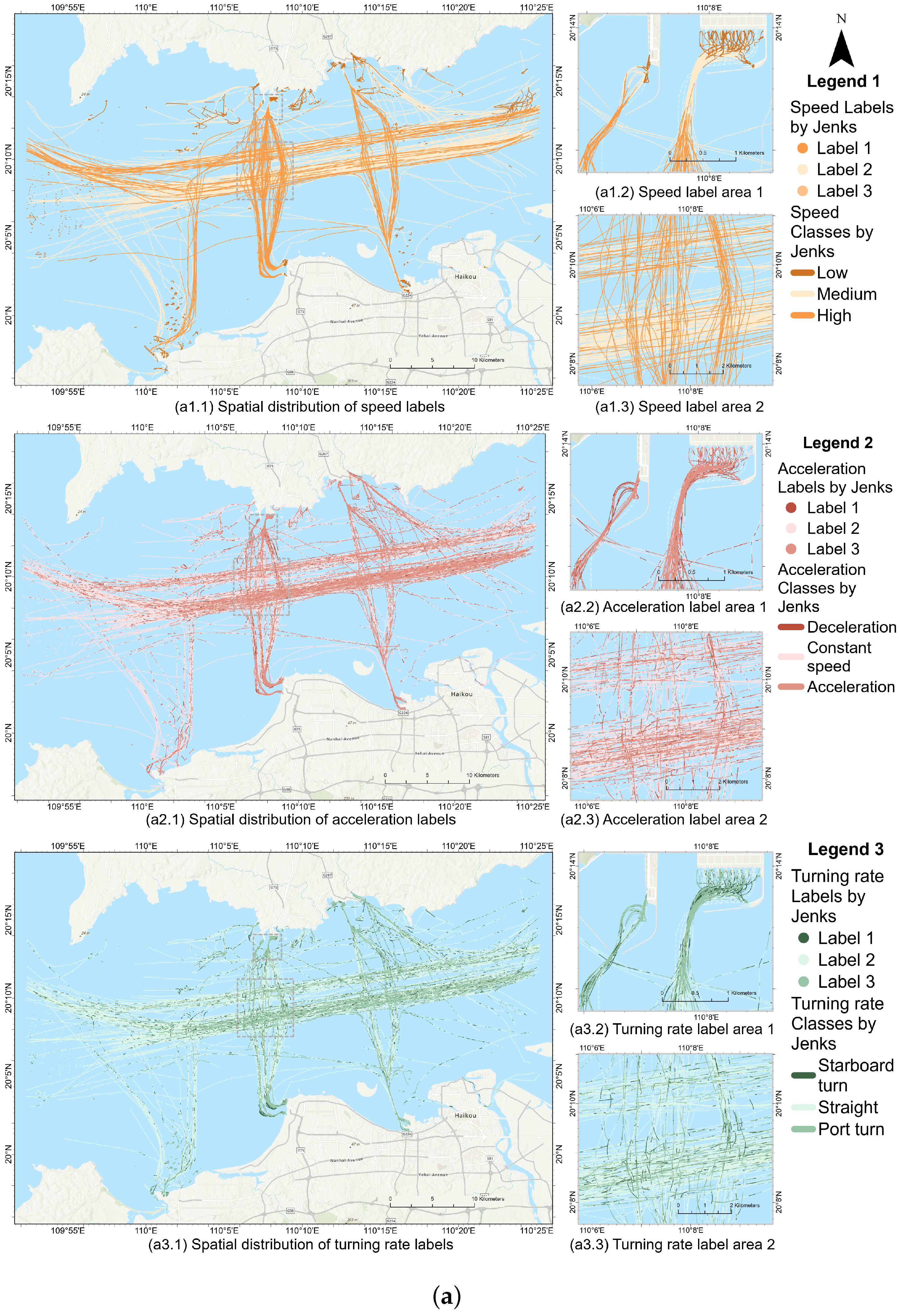
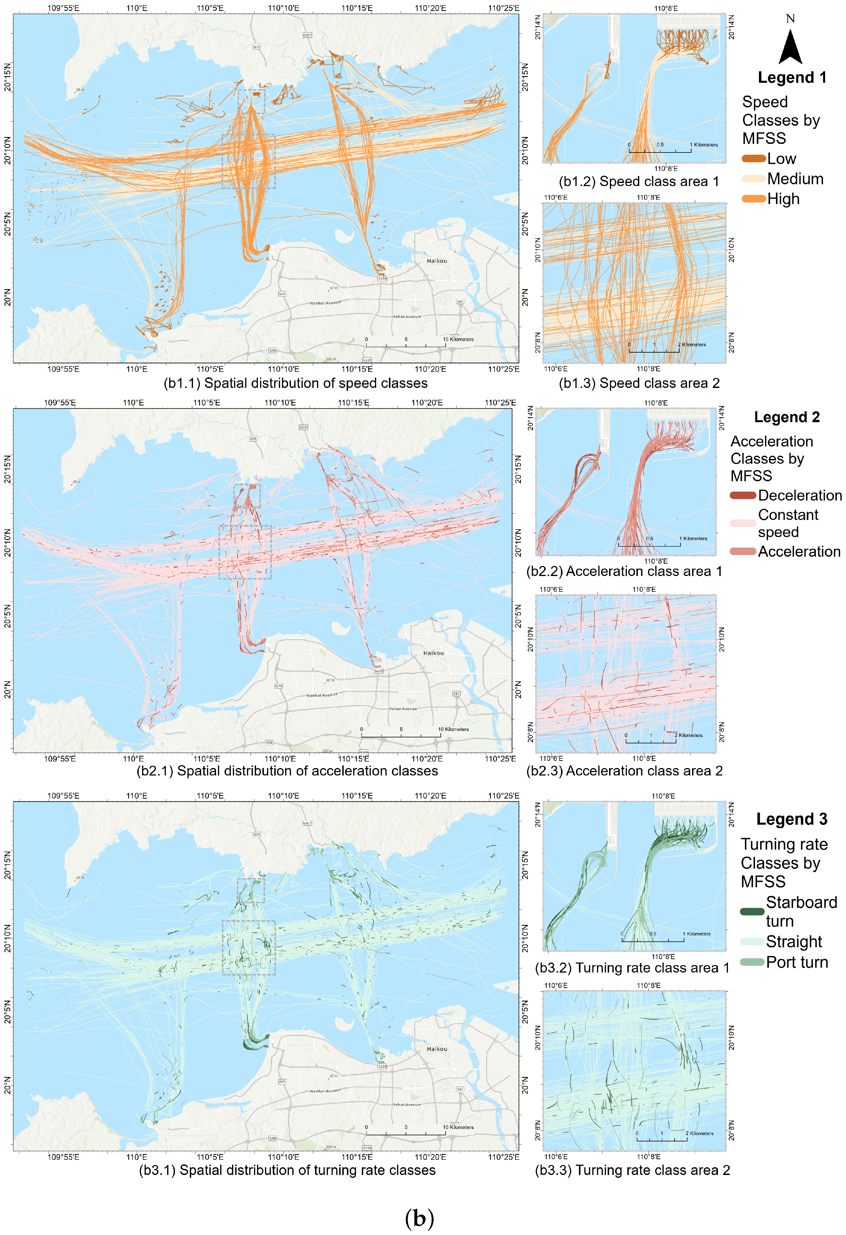
Figure 10 illustrates the trajectory movement patterns with feature labels and behavioral classes. Three movement features, speed, acceleration, and turning rate, were each grouped into three classes to distinguish different behavioral modes. Speed was classified as low, medium, and high. Acceleration was divided into deceleration, constant speed, and acceleration states. The turning rate was described as starboard turn (i.e., turning right), straight (i.e., going forward), and port turn (i.e., turning left). For each feature, three sub-panels are presented with a global overview of the full study area, a focus area 1 on major passenger and cargo ports (Yuehaitie North and Xuwen Port), and an area 2 with the intersection of north–south and east–west shipping lanes within the Traffic Separation Scheme (TSS). This combination provides a representative depiction of commercial vessel movement patterns across the region. The pointwise labels produced by Jenks are shown in Figure 10a as a reference, and the interval behavioral classes produced by MFSS are shown in Figure 10b so that the two methods can be compared directly.

Speed shows a clear spatial pattern and similarity between Jenks and MFSS in the broad zoning of low, medium and high speed regions. Both methods identify low speeds near coastal and anchorage areas while medium to high speeds are observed along main shipping lanes, which confirms that multi-feature segmentation in MFSS does not sacrifice single-feature performance. Compared with Jenks, MFSS better preserves extended low-speed intervals near ports and yields smoother low-to-high or high-to-low changes in areas with frequent speed changes, as visible in panels (a1.2) and (b1.2). This behavior indicates that MFSS retains the principal speed structure while reducing pointwise fragmentation at transition points.

Acceleration exhibits greater variability than speed due to manual operation, wind, and current effects, resulting in more scattered behavioral classes. Jenks tends to fragment acceleration into many short segments because it classifies points independently without considering temporal context. MFSS suppresses noisy spikes and extracts longer, semantically coherent acceleration and deceleration intervals. This is especially evident in port areas where prolonged approach decelerations and departure accelerations are retained, and at corridor intersections where avoidance maneuvers form coherent acceleration patterns, see panels (a2.2), (a2.3) and (b2.2), (b2.3). These results show that MFSS distinguishes genuine maneuvers from transient fluctuations and thus produces segments that better reflect intentional speed changes.

The segmentation of the turning rate shows similar improvements in MFSS. Higher turning frequency occurs in port waters compared to main lanes, reflecting distinct entry and exit maneuvers. In the main channel, while Jenks may treat isolated heading fluctuations as separate turning events and thereby fragment straight-sailing intervals, MFSS filters transient course noise and reconstructs extended straight segments. In port waters, MFSS separates inbound and outbound turning sequences more clearly, and at lane crossings, it identifies continuous avoidance turns associated with interacting north–south and east–west traffic, as shown in panels (a3.1)–(a3.3) and (b3.1)–(b3.3). Overall, MFSS reduces false positive turning events and yields turning segments that are more consistent with vessel maneuvering.

These comparisons show the practical difference between pointwise clustering and segment-based segmentation. Jenks provides pointwise interpretable labels and is useful as a behavioral reference, but it does not enforce temporal continuity and, therefore, can produce highly fragmented segments for noisy features. MFSS combines multiple features and temporal constraints to reduce noise-driven fragmentation and to produce longer segments with clear behavioral meaning because this method emphasizes sustained behaviors rather than transient numerical fluctuations.

4.5.3. Trajectory Segment Behaviors

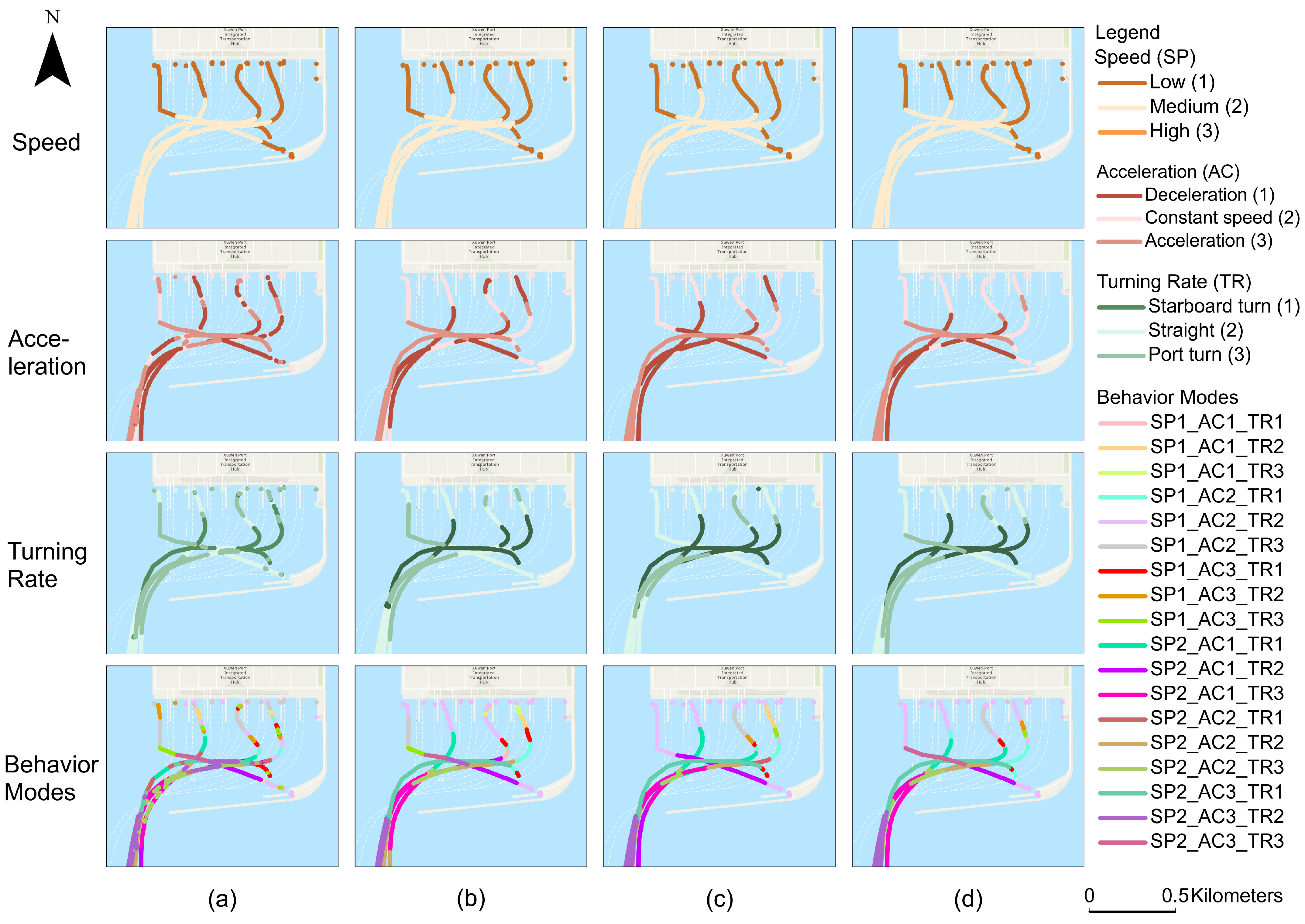
Figure 11 presents a comparison of segmentation results in the Xuwen port area using a one-hour vessel trajectory. The segmentation outcomes generated by Jenks, MFSS, SWS, and TDS are visualized for each movement feature, as well as for the combined behavioral modes. Jenks serves as a baseline, as it classifies pointwise feature values independently for each movement attribute. In contrast, the other three methods perform time-series segmentation by jointly considering all three movement attributes, which may introduce mutual influence among them. This visual comparison enables a clear evaluation of how the four approaches differ in identifying variations in speed (SP), acceleration (AC), turning rate (TR), and the derived integrated behavioral modes.

Speed patterns are relatively stable and continuous in port approaches and along channel lanes, and all three time-series segmenters succeed in separating low-speed berth states from medium-speed channel transit. Differences between methods arise at transition boundaries between low and medium speeds. MFSS produces boundaries that are closest to the Jenks classification, which indicates that MFSS preserves speed consistency more effectively than the other two segmenters. SWS and TDS tend to place boundaries differently in transition zones, producing slightly different segment delimitation that reflects local thresholding or recursive-split choices.

Acceleration and turning rate are inherently more variable, and Jenks yields highly fragmented labels in noisy regions. Time-series segmenters show larger deviations from Jenks in those areas. MFSS focuses on within-segment homogeneity and between-segment distinctness, so it suppresses brief, noisy spikes and captures sustained maneuvers. Consequently, MFSS detects subtle but meaningful transitions that SWS and TDS sometimes miss, especially near the channel entrance and inside turning basins. SWS and TDS are more sensitive to abrupt local changes and, therefore, may fragment intentional maneuvers or overlook small but systematic shifts near berths.

Behavior-mode patterns in the port area are assigned by majority voting over the three feature labels within each segment according to Equation (26). In the main channel, the dominant modes are SP2_AC3_TR2, SP2_AC1_TR2 and SP2_AC2_TR2, representing medium speed with accelerating straight, medium speed with decelerating straight and medium speed with steady straight behavior, respectively. MFSS produces behavior-mode partitions in these channel sections that are closer to the Jenks reference than those from SWS or TDS. SWS tends to merge steady cruising and accelerating segments, while TDS sometimes fails to effectively distinguish between straight channel navigation and local turns near the channel entrance, producing improbable SP2_AC1_TR3 mode for straight segments. In the turning basins, most inbound and outbound maneuvers appear as SP2_AC1_TR3 for inbound decelerating port turns and SP2_AC3_TR1 for outbound accelerating starboard turns, and all three time-series methods detect these turning behaviors, but MFSS yields more contiguous and interpretable turn segments. Near berths, MFSS provides refined yet coherent segment sequences, allowing observation of transitions such as SP1_AC1_TR3 to SP1_AC2_TR2 to SP1_AC3_TR1, which correspond to low-speed accelerating turns, low-speed straight transits and low-speed accelerating turns during departure. This finer resolution allows for identifying berth approach and departure as continuous maneuver sequences. It avoids the limitations of fragmented pointwise labels (Jenks) and over-merged segments that combine distinct yet similar behaviors (SWS and TDS). As a result, MFSS offers a clearer representation of vessel activities in complex port areas.

The case study demonstrates that MFSS produces segmentation that is both semantically meaningful and practically useful. Compared with SWS and TDS, MFSS better balances stability in slow speed zones, robustness to noisy acceleration and heading fluctuations, and clarity of behavior-mode boundaries. These properties make MFSS more suitable for downstream tasks that operate on time intervals, such as anomaly detection, traffic risk assessment, and movement pattern summarization, where coherent and interpretable segments improve reliability and reduce false alarms.

4.6. Sensitivity Analysis

4.6.1. Feature Class Selection

The selection of the class number K for Jenks discretization balances statistical compactness with semantic interpretability. We determined the reasonable class number by integrating quantitative metrics and domain-specific constraints.

We conducted a sensitivity analysis using the Elbow Method, Akaike Information Criterion (AIC), and Bayesian Information Criterion (BIC). To ensure that the evaluation represented diverse maneuvering characteristics, trajectory samples were uniformly extracted across different vessel types. Figure 12 presents the evaluation results for speed, acceleration, and turning rate as K varies from 2 to 6.

The Elbow Method in Figure 12a shows a significant reduction in the Sum of Squared Errors (SSE) as K increases from 2 to 3. The curve exhibits a distinct elbow point at $K=3$, after which the marginal gain in variance reduction diminishes. Concurrently, the AIC and BIC scores in Figure 12b,c demonstrate that $K=3$ achieves a favorable trade-off between model accuracy and complexity. While higher K values yield lower error scores, they significantly increase computational burden for massive AIS datasets without providing proportional behavioral distinctiveness.

Beyond statistical metrics, the choice of $K=3$ is justified by interpretability and operational context. First, discretizing features into three levels (e.g., low, medium, high) aligns with intuitive navigation concepts. This configuration generates $27\left(3^3\right)$ combined behavioral modes, which provides sufficient granularity to capture complex maneuvering patterns while avoiding semantic redundancy. Second, regarding the specific context of the Qiongzhou Strait, maritime regulations impose a speed limit of approximately 12 knots. A three-level discretization adequately captures the essential speed variations (such as berthing, maneuvering, and cruising) within this constrained operational range. Consequently, $K=3$ is selected as the best parameter for this study.

4.6.2. Parameter Selection and Justification of MFSS

The performance of the proposed MFSS algorithm relies on the appropriate setting of hyperparameters, particularly the initial fixed set size $f_{init}$. This parameter governs the balance between the exploration of new subspaces and the exploitation required to refine the current solution. A larger $f_{init}$ restricts the search space for the MIP solver to accelerate computation but may lead to premature convergence. Conversely, a smaller $f_{init}$ expands the search space and increases the computational burden. Given the time limit imposed on the solver, an excessive search space may prevent the discovery of improved solutions and result in ineffective exploration.

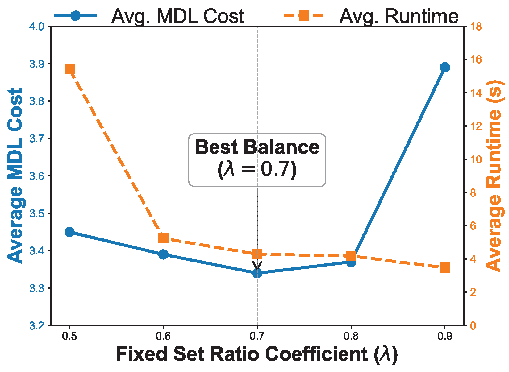
To determine the best configuration, we conducted a sensitivity analysis on the coefficient $\lambda$, which defines the initial fixed set size $f_{init}=\lambda m$, where m is the number of segments. This strategy preserves high-quality segments within the known solution and targets only the less effective sections for re-segmentation. We varied $\lambda$ from 0.5 to 0.9 with a step size of 0.1 using a test dataset comprising 50 trajectory points. To mitigate the stochastic nature of the matheuristic framework, we performed 10 independent runs with different random seeds for each parameter setting. The average MDL cost and average runtime are recorded as performance indicators in Figure 13.

Figure 13 illustrates the trade-off between solution quality and efficiency. The results indicate that when $\lambda <0.6$, the algorithm requires excessive runtime due to the large search space in the MIP phase without yielding a proportionate improvement in MDL reduction. In contrast, setting $\lambda >0.8$ degrades solution quality as the tightly constrained search space causes the algorithm to become trapped in local optima. The configuration with $\lambda =0.7$ identifies the best operating point by achieving the lowest average MDL cost while maintaining reasonable computational time. Consequently, we establish $f_{init}=0.7m$ for all experiments to ensure a robust balance between segmentation accuracy and efficiency.

4.6.3. Problem Complexity and Computational Efficiency

The computational complexity of the proposed framework is governed by the MIP formulation defined in Equations (14)–(20). Structurally, this optimization problem is analogous to the Quadratic Knapsack Problem (QKP), where the objective function accounts for both the linear costs of individual items (segments) and the quadratic interaction profits between pairs of selected items (adjacent segments). Let $M=|C_p|$ denote the number of candidate points. The decision variable $y_{izj}$ effectively linearizes the quadratic term $x_{iz}·x_{zj}$, representing the pairwise dependency between consecutive segments. Consequently, the number of such interaction terms scales with $\mathcal{O}\left(M^3\right)$. As established in the seminal work on combinatorial optimization [56], the QKP is NP-hard since it generalizes the classical Knapsack Problem and contains the Maximum Clique Problem as a special case [57]. This intrinsic complexity makes exact solution methods computationally prohibitive as M increases, thereby necessitating the use of the proposed MFSS framework to efficiently navigate the solution space.

To address this computational challenge, practical efficiency is ensured through a dual mechanism involving data reduction and algorithmic decomposition. The preprocessing phase significantly lowers the problem dimension by extracting only key feature points, ensuring that the number of decision nodes M remains far smaller than the raw trajectory size N ($M\ll N$). Moreover, the MFSS framework employs a fixed-set search strategy that functions as a decomposition mechanism. By restricting the optimization scope to a manageable subspace in each iteration, it enables the exact solver to fully explore the solution space within limited time bounds, thereby bypassing the prohibitive computational burden of a global exact search. To quantify these efficiency gains and validate the solution quality, we compared the proposed MFSS against the standard exact solver CPLEX across varying candidate set sizes, with the maximum runtime limit of 600 s. The results, detailing the MDL costs, relative gaps, and runtime performance, are summarized in

Table 3. MDL costs comparison between CPLEX and the proposed heuristic method under different point set sizes. Runtime is reported in seconds.

Points	Cplex			MFSS
	MDL	Runtime		Avg MDL	Best MDL	Avg Gap	Best Gap	Runtime
50	3.11	109.03		3.11	3.11	0.00%	0.00%	4.29
100	4.11	600.00		3.88	3.85	−5.60%	−6.33%	28.15
200	4.99	600.00		4.74	4.60	−5.01%	−7.81%	139.14

.

As indicated in Table 3, for small-scale instances ($M=50$), both methods converge to the same optimal solution, yet MFSS is approximately 25 times faster. However, as the problem scale increases to 100 and 200 points, the intrinsic complexity of the path-constrained quadratic knapsack structure prevents the exact solver from converging within the time limit. Consequently, CPLEX returns suboptimal solutions with higher MDL costs. In contrast, MFSS achieves superior solution quality (lower MDL values, indicated by negative gaps) with significantly reduced runtime. This efficiency is attributed to the fixed-set decomposition strategy within MFSS. By fixing a subset of segments and optimizing only the remaining subproblem, MFSS allows the underlying CPLEX solver to operate on manageable search spaces. This approach effectively combines the precision of exact solvers with the scalability of heuristics, avoiding the computational bottleneck of global optimization.

5. Conclusions

This study proposes a clustering-aided matheuristic framework to improve generality, robustness and interpretability for behavioral segmentation of AIS trajectories. The framework first decomposes speed, acceleration and turning rate with Jenks algorithm to obtain key feature points as candidate boundaries and pointwise feature labels. These candidate boundaries are then processed by a Matheuristic Fixed Set Search algorithm that minimizes a Minimum Description Length objective to capture behavioral segments. This unsupervised framework divides AIS trajectories without predefined thresholds or labels, making it resilient to the noisy nature of AIS data and applicable across diverse vessel types and waterways. Integrating the upstream clustering step with the downstream matheuristic search algorithm enhances efficiency and ensures the interpretability of identified behavioral segments. Experiments on AIS data from the Qiongzhou Strait show that the framework can successfully partition vessel trajectories into semantically coherent segments. Compared to established baselines, the proposed method achieves a superior trade-off between the homogeneity within segments and distinctness across segments, while preserving dominant behavioral patterns.

Building upon these results, this work advances maritime trajectory analysis by further exploring semantic behavioral discovery. The novel formulation using multi-dimensional kinematic features without geometric factors and the MDL principle establishes a generalized framework that remains robust across varying vessel types and data quality. Furthermore, the developed matheuristic strategy successfully strikes an effective balance between theoretical optimization precision and the computational efficiency required for large-scale data processing. In the context of practical application, this framework functions as an offline knowledge discovery engine for processing historical AIS streams. At the microscopic level, the derived semantic segments serve as high-quality behavioral samples for calibrating trajectory prediction models and identifying navigation anomalies. From a mesoscopic perspective, these coherent segments facilitate the extraction of representative routes to support port scheduling and operational efficiency assessments. On a macroscopic scale, the identified maneuvering patterns provide a data-driven basis for regional risk analysis when combined with standard protocols such as the International Regulations for Preventing Collisions at Sea (COLREGs).

Despite these contributions, the current framework presents certain limitations. The analysis is currently confined to kinematic features without integrating environmental contexts such as waterway regulations or traffic interactions, thereby restricting the higher-level causal interpretation of the identified behaviors. Regarding the data-driven discretization, the determination of reasonable feature classes depends on the specific statistical distribution of the input dataset. While the framework is designed for broad applicability, transferring the model to maritime environments with distinct operational profiles may require recalibrating the discretization parameters to ensure semantic accuracy. Furthermore, the computational complexity inherent to the MDL objective and MIP solver restricts the current implementation to offline batch processing, limiting its direct deployment for real-time analysis of global-scale streams.

Future research will extend this work in ways that enhance both methodological capability and application breadth. A natural direction is to enrich the segmentation process with contextual factors such as waterway constraints [58], vessel categories and traffic interactions, so that the identified segments reflect not only movement patterns but also the operational intentions that shape them. Another improvement lies in developing adaptive schemes for discretization and search configurations, allowing the framework to adjust automatically to variations in data distribution and navigational environments rather than relying on manual parameter tuning. Progress in computational efficiency is also essential, where incremental evaluation of MDL terms or approximate optimization strategies could support faster processing and move the framework toward online use. Beyond these algorithmic advances, future work may further integrate the resulting behavioral segments into downstream tasks such as prediction, anomaly detection and regional risk assessment, enabling a more complete pipeline for maritime intelligence. Broader validation in diverse waterways and collaboration with operational stakeholders will help translate these improvements into practical maritime monitoring systems.

References

1. Zhang, C.; Liu, S.; Guo, M.; Liu, Y. A novel ship trajectory clustering analysis and anomaly detection method based on AIS data. Ocean Eng. 2023, 288, 116082. [Google Scholar] [CrossRef]
2. Gao, D.W.; Zhu, Y.S.; Zhang, J.F.; He, Y.K.; Yan, K.; Yan, B.R. A novel MP-LSTM method for ship trajectory prediction based on AIS data. Ocean Eng. 2021, 228, 108956. [Google Scholar] [CrossRef]
3. Ma, Q.; Tang, H.; Liu, C.; Zhang, M.; Zhang, D.; Liu, Z.; Zhang, L. A big data analytics method for the evaluation of maritime traffic safety using automatic identification system data. Ocean Coast. Manag. 2024, 251, 107077. [Google Scholar] [CrossRef]
4. Liu, D.; Rong, H.; Soares, C.G. Shipping route modelling of AIS maritime traffic data at the approach to ports. Ocean Eng. 2023, 289, 115868. [Google Scholar] [CrossRef]
5. Zhang, S.K.; Shi, G.Y.; Liu, Z.J.; Zhao, Z.W.; Wu, Z.L. Data-driven based automatic maritime routing from massive AIS trajectories in the face of disparity. Ocean Eng. 2018, 155, 240–250. [Google Scholar] [CrossRef]
6. Liu, C.; Liu, J.; Zhou, X.; Zhao, Z.; Wan, C.; Liu, Z. AIS data-driven approach to estimate navigable capacity of busy waterways focusing on ships entering and leaving port. Ocean Eng. 2020, 218, 108215. [Google Scholar] [CrossRef]
7. Zhang, R.; Dong, D.; Chen, X.; Zhang, B.; Zhang, Y.; Ye, L.; Liu, B.; Zhao, Y.; Peng, C. AIS data-driven analysis for identifying cargo handling events in international trade tankers. Ocean Eng. 2025, 317, 120016. [Google Scholar] [CrossRef]
8. Zheng, Y. Trajectory data mining: An overview. ACM Trans. Intell. Syst. Technol. TIST 2015, 6, 1–41. [Google Scholar] [CrossRef]
9. Izakian, Z.; Mesgari, M.S.; Weibel, R. A feature extraction based trajectory segmentation approach based on multiple movement parameters. Eng. Appl. Artif. Intell. 2020, 88, 103394. [Google Scholar] [CrossRef]
10. Laube, P.; Imfeld, S.; Weibel, R. Discovering relative motion patterns in groups of moving point objects. Int. J. Geogr. Inf. Sci. 2005, 19, 639–668. [Google Scholar] [CrossRef]
11. Alvares, L.O.; Bogorny, V.; Kuijpers, B.; de Macedo, J.A.F.; Moelans, B.; Vaisman, A. A model for enriching trajectories with semantic geographical information. In Proceedings of the 15th Annual ACM International Symposium on Advances in Geographic Information Systems, Seattle WA, USA, 7–9 November 2007; pp. 1–8. [Google Scholar]
12. Palma, A.T.; Bogorny, V.; Kuijpers, B.; Alvares, L.O. A clustering-based approach for discovering interesting places in trajectories. In Proceedings of the ACM symposium on Applied computing, Fortaleza, CE, Brazil, 16–20 March 2008; pp. 863–868. [Google Scholar]
13. Soares Júnior, A.; Moreno, B.N.; Times, V.C.; Matwin, S.; Cabral, L.d.A.F. GRASP-UTS: An algorithm for unsupervised trajectory segmentation. Int. J. Geogr. Inf. Sci. 2015, 29, 46–68. [Google Scholar] [CrossRef]
14. Aminikhanghahi, S.; Cook, D.J. A survey of methods for time series change point detection. Knowl. Inf. Syst. 2017, 51, 339–367. [Google Scholar] [CrossRef] [PubMed]
15. Buchin, M.; Driemel, A.; Van Kreveld, M.J.; Sacristán, V. Segmenting trajectories: A framework and algorithms using spatiotemporal criteria. J. Spat. Inf. Sci. 2011, 3, 33–63. [Google Scholar]
16. Liu, C.; Wang, J.; Liu, A.; Cai, Y.; Ai, B. An asynchronous trajectory matching method based on piecewise space-time constraints. IEEE Access 2020, 8, 224712–224728. [Google Scholar] [CrossRef]
17. Landsea, C.W.; Franklin, J.L. Atlantic hurricane database uncertainty and presentation of a new database format. Mon. Weather Rev. 2013, 141, 3576–3592. [Google Scholar] [CrossRef]
18. Etemad, M.; Etemad, Z.; Soares, A.; Bogorny, V.; Matwin, S.; Torgo, L. Wise sliding window segmentation: A classification-aided approach for trajectory segmentation. In Proceedings of the Advances in Artificial Intelligence: 33rd Canadian Conference on Artificial Intelligence, Canadian AI 2020, Ottawa, ON, Canada, 13–15 May 2020; Proceedings 33. Springer: Berlin/Heidelberg, Germany, 2020; pp. 208–219. [Google Scholar]
19. Junior, A.S.; Times, V.C.; Renso, C.; Matwin, S.; Cabral, L.A. A semi-supervised approach for the semantic segmentation of trajectories. In Proceedings of the 19th IEEE international conference on mobile data management (MDM), Aalborg, Denmark, 26–28 June 2018; IEEE: Piscataway, NJ, USA, 2018; pp. 145–154. [Google Scholar]
20. Ye, L.; Chen, X.; Zhang, R.; Zhang, B.; Liu, H. An adaptive trajectory segmentation and simplification algorithm based on vessel behavioral features. Ocean Eng. 2024, 312, 119329. [Google Scholar] [CrossRef]
21. Etemad, M.; Soares, A.; Etemad, E.; Rose, J.; Torgo, L.; Matwin, S. SWS: An unsupervised trajectory segmentation algorithm based on change detection with interpolation kernels. GeoInformatica 2021, 25, 269–289. [Google Scholar] [CrossRef]
22. Dodge, S.; Laube, P.; Weibel, R. Movement similarity assessment using symbolic representation of trajectories. Int. J. Geogr. Inf. Sci. 2012, 26, 1563–1588. [Google Scholar] [CrossRef]
23. Yu, Z.; Wu, H.; Yin, Z.; Liu, K.; Zhang, R. Vessel trajectory segmentation: A survey. In Proceedings of the International Conference on Database Systems for Advanced Applications, Tianjin, China, 17 April 2023; Springer: Berlin/Heidelberg, Germany, 2023; pp. 166–180. [Google Scholar]
24. Douglas, D.H.; Peucker, T.K. Algorithms for the reduction of the number of points required to represent a digitized line or its caricature. Cartogr. Int. J. Geogr. Inf. Geovisualization 1973, 10, 112–122. [Google Scholar] [CrossRef]
25. Ma, L.; Shi, G.; Li, W.; Jiang, D. A direction-preserved vessel trajectory compression algorithm based on open window. J. Mar. Sci. Eng. 2023, 11, 2362. [Google Scholar] [CrossRef]
26. Keogh, E.; Chu, S.; Hart, D.; Pazzani, M. An online algorithm for segmenting time series. In Proceedings of the IEEE International Conference on Data Mining, San Jose, CA, USA, 29 November–2 December 2001; IEEE: Piscataway, NJ, USA, 2001; pp. 289–296. [Google Scholar]
27. Lin, K.; Xu, Z.; Qiu, M.; Wang, X.; Han, T. Noise filtering, trajectory compression and trajectory segmentation on GPS data. In Proceedings of the 11th International Conference on Computer Science & Education (ICCSE), Nagoya, Japan, 23–25 August 2016; IEEE: Piscataway, NJ, USA, 2016; pp. 490–495. [Google Scholar]
28. Amigo, D.; Pedroche, D.S.; García, J.; Molina, J.M. Segmentation optimization in trajectory-based ship classification. J. Comput. Sci. 2022, 59, 101568. [Google Scholar] [CrossRef]
29. Leiva, L.A.; Vidal, E. Warped k-means: An algorithm to cluster sequentially-distributed data. Inf. Sci. 2013, 237, 196–210. [Google Scholar] [CrossRef]
30. Birant, D.; Kut, A. ST-DBSCAN: An algorithm for clustering spatial–temporal data. Data Knowl. Eng. 2007, 60, 208–221. [Google Scholar] [CrossRef]
31. Chen, W.; Ji, M.; Wang, J. T-DBSCAN: A Spatiotemporal Density Clustering for GPS Trajectory Segmentation. Int. J. Online Eng. 2014, 10, 19–24. [Google Scholar] [CrossRef]
32. Rissanen, J. Modeling by shortest data description. Automatica 1978, 14, 465–471. [Google Scholar] [CrossRef]
33. Lee, J.G.; Han, J.; Whang, K.Y. Trajectory clustering: A partition-and-group framework. In Proceedings of the ACM SIGMOD International Conference on Management of Data, Beijing, China, 12–14 June 2007; pp. 593–604. [Google Scholar]
34. Etemad, M.; Júnior, A.S.; Hoseyni, A.; Rose, J.; Matwin, S. A Trajectory Segmentation Algorithm Based on Interpolation-based Change Detection Strategies. In Proceedings of the EDBT/ICDT Workshops, Lisbon, Portugal, 26 March 2019; Volume 31, p. 6. [Google Scholar]
35. Zheng, Y.; Zhang, L.; Ma, Z.; Xie, X.; Ma, W.Y. Recommending friends and locations based on individual location history. ACM Trans. Web TWEB 2011, 5, 1–44. [Google Scholar] [CrossRef]
36. Guo, S.; Li, X.; Ching, W.K.; Dan, R.; Li, W.K.; Zhang, Z. GPS trajectory data segmentation based on probabilistic logic. Int. J. Approx. Reason. 2018, 103, 227–247. [Google Scholar] [CrossRef]
37. Xiang, L.; Gao, M.; Wu, T. Extracting stops from noisy trajectories: A sequence oriented clustering approach. ISPRS Int. J.-Geo-Inf. 2016, 5, 29. [Google Scholar] [CrossRef]
38. Liu, M.; He, G.; Long, Y. A semantics-based trajectory segmentation simplification method. J. Geovisualization Spat. Anal. 2021, 5, 19. [Google Scholar] [CrossRef]
39. Li, J.; Liu, H.; Chen, X.; Li, J.; Xiang, J. Vessel pattern recognition using trajectory shape feature. In Proceedings of the 5th International Conference on Computer Science and Artificial Intelligence, Beijing, China, 4–6 December 2021; pp. 84–90. [Google Scholar]
40. Yan, W.; Wen, R.; Zhang, A.N.; Yang, D. Vessel movement analysis and pattern discovery using density-based clustering approach. In Proceedings of the IEEE international conference on big data (Big Data), Washington, DC, USA, 5–8 December 2018; IEEE: Piscataway, NJ, USA; 2016, pp. 3798–3806. [Google Scholar]
41. Rocha, J.A.M.; Times, V.C.; Oliveira, G.; Alvares, L.O.; Bogorny, V. DB-SMoT: A direction-based spatio-temporal clustering method. In Proceedings of the 5th IEEE International Conference Intelligent Systems, London, UK, 7–9 July 2010; IEEE: Piscataway, NJ, USA, 2010; pp. 114–119. [Google Scholar]
42. Wu, S.; Zimányi, E.; Sakr, M.; Torp, K. Semantic segmentation of ais trajectories for detecting complete fishing activities. In Proceedings of the 23rd IEEE International Conference on Mobile Data Management (MDM), Paphos, Cyprus, 6–9 June 2022; IEEE: Piscataway, NJ, USA, 2022; pp. 419–424. [Google Scholar]
43. Das, R.D.; Winter, S. Automated urban travel interpretation: A bottom-up approach for trajectory segmentation. Sensors 2016, 16, 1962. [Google Scholar] [CrossRef]
44. Zhao, B.; Liu, M.; Han, J.; Ji, G.; Liu, X. Efficient semantic enrichment process for spatiotemporal trajectories. Wirel. Commun. Mob. Comput. 2021, 2021, 4488781. [Google Scholar] [CrossRef]
45. Gao, Y.; Huang, L.; Feng, J.; Wang, X. Semantic trajectory segmentation based on change-point detection and ontology. Int. J. Geogr. Inf. Sci. 2020, 34, 2361–2394. [Google Scholar] [CrossRef]
46. Wen, Y.; Zhang, Y.; Huang, L.; Zhou, C.; Xiao, C.; Zhang, F.; Peng, X.; Zhan, W.; Sui, Z. Semantic modelling of ship behavior in harbor based on ontology and dynamic bayesian network. ISPRS Int. J. Geo-Inf. 2019, 8, 107. [Google Scholar] [CrossRef]
47. Gao, J.; Cai, Z.; Yu, W.; Sun, W. Trajectory data compression algorithm based on ship navigation state and acceleration variation. J. Mar. Sci. Eng. 2023, 11, 216. [Google Scholar] [CrossRef]
48. Gharghabi, S.; Ding, Y.; Yeh, C.C.M.; Kamgar, K.; Ulanova, L.; Keogh, E. Matrix profile VIII: Domain agnostic online semantic segmentation at superhuman performance levels. In Proceedings of the IEEE International Conference on Data Mining (ICDM), New Orleans, LA, USA, 18–21 November 2017; IEEE: Piscataway, NJ, USA, 2017; pp. 117–126. [Google Scholar]
49. Xu, W.; Dong, S. Application of artificial intelligence in an unsupervised algorithm for trajectory segmentation based on multiple motion features. Wirel. Commun. Mob. Comput. 2022, 2022, 9540944. [Google Scholar] [CrossRef]
50. Li, G.; Liu, M.; Zhang, X.; Wang, C.; Lai, K.h.; Qian, W. Semantic recognition of ship motion patterns entering and leaving port based on topic model. J. Mar. Sci. Eng. 2022, 10, 2012. [Google Scholar] [CrossRef]
51. Huang, L.; Wen, Y.; Guo, W.; Zhu, X.; Zhou, C.; Zhang, F.; Zhu, M. Mobility pattern analysis of ship trajectories based on semantic transformation and topic model. Ocean Eng. 2020, 201, 107092. [Google Scholar] [CrossRef]
52. Chen, J.; Yang, S.; Li, H.; Zhang, B.; Lv, J. Research on geographical environment unit division based on the method of natural breaks (Jenks). Int. Arch. Photogramm. Remote Sens. Spat. Inf. Sci. 2013, 40, 47–50. [Google Scholar] [CrossRef]
53. Grünwald, P.D. The Minimum Description Length Principle; MIT Press: Cambridge, MA, USA, 2007. [Google Scholar]
54. Jovanovic, R.; Tuba, M.; Voß, S. Fixed set search applied to the traveling salesman problem. In Proceedings of the International Workshop on Hybrid Metaheuristics, Málaga, Spain, 20–22 June 2018; Springer: Berlin/Heidelberg, Germany, 2018; pp. 63–77. [Google Scholar]
55. Jovanovic, R.; Voß, S. Fixed set search matheuristic applied to the knapsack problem with forfeits. Comput. Oper. Res. 2024, 168, 106685. [Google Scholar] [CrossRef]
56. Gallo, G.; Hammer, P.L.; Simeone, B. Quadratic Knapsack Problems. Math. Program. 1980, 12, 132–149. [Google Scholar]
57. Jovanovic, R.; Voß, S. Solving the Quadratic Knapsack Problem Using GRASP. In Metaheuristics for Machine Learning: New Advances and Tools; Springer: Berlin/Heidelberg, Germany, 2022; pp. 157–178. [Google Scholar]
58. Lalla-Ruiz, E.; Shi, X.; Voß, S. The waterway ship scheduling problem. Transp. Res. Part D Transp. Environ. 2018, 60, 191–209. [Google Scholar] [CrossRef]
Figure 1. Feature profiles of trajectory. (a) Trajectory location; (b) Speed over time; (c) Acceleration over time; (d) Turning rate over time.
Jmse 13 02393 g001
Figure 2. Profile decomposition of a trajectory based on Jenks, using speed as a representative feature. (a) Speed variation over time; (b) Speed histogram illustrating Jenks breaks; (c) Speed over time colored by feature labels. The distinct colors (orange, red, and green) represent different feature labels, where trajectory points are classified into specific label categories based on their speed values.
Jmse 13 02393 g002
Figure 3. Key feature points extraction and aggregation. (a) Trajectory showing the union of all key feature points from three profiles; (b) Key feature points derived from speed; (c) Key feature points derived from acceleration; (d) Key feature points derived from turning rate. For each attribute, a key feature point is defined when a label change occurs between consecutive points. The final candidate set in (a) is formed by the union of the sets shown in (bd), where a single trajectory point may simultaneously correspond to key feature points across different attributes.
Jmse 13 02393 g003
Figure 4. Example of behavioral trajectory segmentation and MDL cost formulation. (a) Visual representation of a trajectory with behavioral segmentation; (b) Corresponding trajectory information table. The numerical example demonstrates the step-by-step calculation of the MDL cost for the given segmentation.
Jmse 13 02393 g004
Figure 5. Study area and spatial distribution of original AIS trajectory points in this case study.
Jmse 13 02393 g005
Figure 6. Comparison of the overall AIS trajectory dataset before and after preprocessing. (a) shows the original data with visible noise and drift; (b) shows the cleaned data with clearer traffic patterns.
Jmse 13 02393 g006
Figure 7. Statistical assessment of AIS data quality and error types. (a) Pie charts showing the proportion of valid vs. cleaned data points; (b) Bar chart detailing the distribution of specific error sources, including spatial duplicate (Spatial Dup), time duplicate (Time Dup), geometric jump (Geo Jump) and behavioral jump (Beh Jump).
Jmse 13 02393 g007
Figure 8. Examples of abnormal trajectory segments with data errors. (a) Position anomaly; (b) Speed anomaly; (c) Heading anomaly. The red points indicate the identified data errors.
Jmse 13 02393 g008
Figure 9. Comparison of trajectory cleaning results before and after handling data errors. Subfigures (a,b) show the trajectory cleaning comparison for MMSI 413699910 and MMSI 413306950, respectively.
Jmse 13 02393 g009
Figure 10. Comparison of trajectory representations based on a twelve-hour sample of cleaned AIS trajectories. Subfigures (a,b) show the results of Jenks-based feature labeling and MFSS-based segment behavioral representations, respectively. For both subfigures, indices (1)–(3) correspond to feature labels and behavioral classes across speed, acceleration, and turning rate, respectively. Within each series, the sub-panels (e.g., .1–.3) represent the whole study area, the port area, and the crossing area, respectively.
Jmse 13 02393 g010aJmse 13 02393 g010b
Figure 11. Comparison of movement patterns and behavior modes in Xuwen Port based on a one-hour sample of cleaned AIS trajectories. The subfigures correspond to the segmentation results obtained by (a) Jenks, (b) MFSS, (c) SWS, and (d) TDS, respectively. For each method, the visualization displays the feature profiles for speed, acceleration, and turning rate, followed by the identified behavior modes.
Jmse 13 02393 g011
Figure 12. Sensitivity analysis for determining the reasonable class number K. (a) The Elbow method based on SSE; (b) The Akaike Information Criterion (AIC) scores; (c) The Bayesian Information Criterion (BIC) scores.
Jmse 13 02393 g012
Figure 13. Sensitivity analysis of the initial fixed set size ( f i n i t ). The blue line and orange line correspond to the average MDL cost and average runtime in seconds, respectively, across varying fixed set size ratios ( λ ).
Jmse 13 02393 g013