Article

MNAT: A Simulation Tool for Underwater Radiated Noise

by
Mohammad Rasoul Tanhatalab
and
Paolo Casari
*
Department of Information Engineering and Computer Science, University of Trento, Via Sommarive 9, Povo, 38123 Trento, Italy
*
Author to whom correspondence should be addressed.
J. Mar. Sci. Eng. 2025, 13(11), 2045; https://doi.org/10.3390/jmse13112045
Submission received: 1 September 2025 / Revised: 21 October 2025 / Accepted: 22 October 2025 / Published: 25 October 2025

Abstract

Shipping expansion, offshore energy generation, fish farming, and construction work radiate high levels of underwater noise, which may critically stress marine ecosystems. Tools for simulating, analyzing, and forecasting underwater noise can be of great help in understanding the impact of underwater radiated noise both on the environment and on man-made equipment, such as underwater communication and telemetry systems. To address this challenge, we developed a web-based Marine Noise Analysis Tool (MNAT) that models, simulates, and predicts underwater radiated noise levels. To reproduce realistic shipping conditions, MNAT combines real-time Automatic Identification System data with environmental data using broadly accepted underwater acoustic propagation models, including Bellhop and RAM. Moreover, MNAT can simulate other kinds of noise sources, such as seismic airguns. It features an intuitive interface enabling real-time tracking, noise impact assessment, and interactive visualizations. MNAT’s noise modeling capabilities allow the user to design resilient communication systems in different noise conditions, analyze maritime noise data, and forecast future noise levels, with potential contributions to the design of noise-resilient systems, to the optimization of environmental monitoring device deployments, and to noise mitigation policymaking. MNAT has been made available for the community at a public GIT repository.

1. Introduction

Underwater noise pollution is becoming more widely acknowledged as a major issue that calls for creative monitoring, analysis, and mitigation approaches [1]. Various techniques based on noise simulation, Passive Acoustic Monitoring (PAM), and predictive algorithms are currently used to analyze radiated noise patterns and their ecological impact. Existing solutions, however, have scalability limitations when processing real-time data and providing the corresponding output to users, leaving a gap open for new systems that efficiently analyze and process underwater noise data.
In response to such issues, this paper presents the MNAT, a web application designed for the real-time simulation, modeling, and prediction of underwater noise propagation. MNAT utilizes current Automatic Identification System (AIS) data (position, properties, and cruising information of vessels at sea) along with oceanic data to estimate underwater noise emissions using acoustic models. The tool incorporates two acoustic propagation models, namely Bellhop and Range-dependent Acoustic Model (RAM) [2], as general-purpose tools that can model acoustic propagation in different marine environments and conditions. MNAT enables a variety of functions, such as real-time tracking, impact analysis of noise, and dynamic visualization.
This paper presents the design and functionalities of MNAT, including the design process and the optimizations applied to improve the speed of acoustic propagation modeling over basin- and sea-level scales. We emphasize that the tool is not tailored to just assessing the impact of noise on communication systems, but rather it can help assess noise in a variety of contexts. These include, e.g., evaluating the average insonification of different sea areas at different frequencies and possibly at different times of day, in order to assess how different marine fauna species are affected by radiated noise.
The remainder of this paper is organized as follows. A review of the relevant literature is presented in Section 2 and structured around three components: underwater acoustic models (Section 2.1), AIS data management and preprocessing (Section 2.2), and available simulation tools for underwater noise analysis (Section 2.3). Section 3 introduces the MNAT architecture and its functionalities. Section 4 discusses two use cases: the first one visualizes and provides noise propagation of vessels (Section 4.1), and the second case presents the analysis of seismic airgun noise propagation (Section 4.2). Finally, Section 5 presents concluding remarks and discusses future work.

2. Related Work

This section presents a survey of the literature in the main areas related to our work. Section 2.1 provides an account of works related to underwater acoustic propagation modeling; Section 2.2 presents methods and applications related to AIS data processing; finally, Section 2.3 surveys other simulation tools for underwater noise analysis.

2.1. Foundations and Advances in Underwater Acoustic Modeling

Underwater acoustic propagation modeling is the foundation for predicting sound behavior in the ocean, with applications in communication, sensing, and environmental monitoring. The field relies heavily on some well-established models.
RAM [3] uses parabolic equations, Bellhop [4] implements a ray-based approach, Kraken employs normal mode analysis for low-frequency propagation, and OASES applies wavenumber integration for layered, range-independent settings [2]. These tools are still being improved to strike a balance between computational demands and accuracy.
One of the main areas of applied modeling is ship-radiated noise. Using simulations and analytical techniques, Zhang and Meng [5] investigated the effects of water depth, seabed characteristics, and ambient noise on ship noise, evaluating the effects on communications and marine life. Neenan et al. [6] used acoustic models and AIS ship-tracking to map noise emissions and pinpoint ecologically sensitive areas. Using a semi-empirical model known as Propulsion-Induced Acoustic Noise at Operating (PIANO) conditions for source levels and ARTEMIA for propagation via the parabolic equation method, the NAVISON project [7] simulated noise from European ship traffic at larger scales. It created sound maps throughout the Baltic, Black, Mediterranean, and North seas as well as the Northeast Atlantic, highlighting the contributions of cargo, container, and tanker vessels while concentrating on frequencies that are important to marine life (63 Hz; 125 Hz).
Comparative research works investigate which propagation models work best in this respect. According to Hartstra et al. [8], Bellhop performs better in deep water at higher frequencies, but its runtime scales with distance, whereas RAM is effective for shallow-water, low-frequency scenarios (up to 11–12 kHz). According to a more comprehensive comparison of RAM, Bellhop, Kraken, and OASES by Ksel et al. [2], RAM and Bellhop are better suited for range-dependent settings, whereas Kraken and OASES work best in stratified, range-independent environments. Both impulsive and long-term noise can be modeled.
In order to inform ecosystem protection, Larayedh et al. [9] used RAM to model shipping noise in the Red sea. Durofchalk et al. [10] used Bellhop-3D to simulate propagation in complex bathymetric conditions like oceanic fronts and seamounts, whereas Laws [11] used RAM-PE to evaluate the impact of pile-driving noise. Quonops integrates RAM and Bellhop to model the environmental impact of shipping and offshore wind farms in terms of noise [12]. Broader issues are also highlighted by recent surveys. Meng et al. [13] noted enduring challenges from environmental variability, noise pollution, and climate change, while emphasizing advancements in acoustic modeling, signal processing, and sensor technology that support communication, navigation, and sensing.
Lastly, ship sources are the focus of specific noise-generation models. A mathematical framework combining propeller cavitation, hull vibrations, and hydrodynamic flow noise was proposed by Prokopovich and Shafranyuk [14]. Their model predicts noise across frequency ranges by fusing theoretical analysis with experimental data.

2.2. Methods and Applications in AIS Data Preprocessing

AIS enables ship tracking, navigation safety, and traffic management in maritime environments. However, raw AIS data are prone to inconsistencies, missing values, and noise. Thus, preprocessing is unavoidable for AIS data analysis to provide meaningful conclusions. The following papers address various approaches and the use of AIS data preprocessing, with a focus on cleaning and structuring AIS information for ship classification and trajectory analysis.
Huang et al. [15] suggest a Machine Learning (ML) classification approach to identify subtypes of cargo ships (such as bulk carriers, vehicle carriers, and container ships) in AIS data. The study combines geometric features, such as ship perimeter and width, along with track data such as speed, and achieves an accuracy of nearly 97%. The method was tested in the Changhua wind farm channel. Feature engineering and the selection of the best machine learning method were performed to optimize ship monitoring at sea, traffic management, as well as out-of-character activity detection. The study, however, was narrowed down to cargo, carrier, and container ships and realized in a channel scenario, which restricts its application to other ship categories and free water contexts.
The approach in [16] initially relies on images taken at port regions as well as aerial images or satellite images. It then utilizes data from AIS, i.e., speed, heading, and dynamic properties for ship classification. Image-based approaches to ship classification generally use unsupervised learning models, especially convolutional neural networks, to extract the important features from the images of ships. However, these methods suffer from some limitations; for example, most of them rely on optical sensors that are not effective under harsh weather conditions or in low light.
The methods in [17] generally involve creating a graphical representation of spatio-temporal data from ship trajectories to enable classification via graphical recognition. For example, some methods transform latitude and longitude data into scatter plots, plot speed as color, and overlap coasts to train deep residual networks for the classification system.
In [18], the authors present a ship classification method for massive AIS trajectories based on Graph Neural Networks (GNNs). Their proposed method converts ship trajectory data into a graph structure by representing track points as vertices and establishing edges based on spatiotemporal features like distance and speed. This GNN is employed to classify ships into four types: fishing vessels, passenger ships, oil tankers, and container ships.
The work in [19] presents a real-time application, such as a navigation safety monitoring system, to extract geometric and motion features from AIS data directly rather than using graphical methods. This study integrates geographical data with static and dynamic AIS features and proposes a classification model comparing random forests and decision trees. The models are tested in Danish waters, showing better performance on fishing boats and passenger ships, although they fail to reliably distinguish cargo ships from oil tankers.
The literature confirms that several challenges still exist when correcting or improving imprecise or incomplete AIS data, specifically concerning the vessel type feature.

2.3. Simulation Tools for Underwater Noise Analysis

Underwater simulation tools are critical for studying sound transmission, performing environmental assessment, and supporting maritime operations. They facilitate passive acoustic observation, noise modeling, and predictive analysis for marine science and ocean management. This section reviews several available tools in this respect.
In [20], the University of Washington’s Ocean Data Lab provided the Ocean Noise Explorer (ONE) web-based tool, which visualizes and analyzes ocean noise data acquired from hydrophone arrays in the Pacific ocean. AcTUP (LITE) [21] is also a research-grade software that serves as the front-end for the Acoustic Toolbox (AT) for simple comparisons of various acoustic propagation models like Bellhop, Kraken, and RAM.
Several methodologies have been established for the acoustic monitoring and assessment of noise impact underwater. BlueOASIS [22] offers analytical tools for the simulation of environmental noise levels and their interactions with marine life.
The UNWAS platform [23] employed a distributed array of hydrophones for the measurement of large-scale ocean noise, to help detect surface and underwater targets. Satellite observation platforms such as Skylight [24] also integrated an AIS and remote sensing imagery to observe vessel movement patterns and their contribution to ocean noise pollution. Noise mapping approaches have also been applied at the regional level. In [25], Indian Ocean Region studies have combined ship traffic density from AIS data with moored buoy measurements to model low-frequency radiated noise in selected maritime areas.
To promote comparability and standardization of studies of underwater noise, analytical tools such as MANTA [26] have been developed. MANTA records metadata and processes acoustic data to make uniform measurements of background noise levels across different datasets. The dBSea tool [27] has also been applied for simulating and visualizing the propagation of underwater noise with environmental factors such as bathymetry, water temperature, and salinity. For this tool, the user needs to set and configure various parameters manually. Furthermore, the tool was not designed to read real-time data and does not combine different sources of noise.
Table 1 presents a comparative analysis of MNAT alongside other selected platforms. In general, currently used tools are based on passive acoustic monitoring, noise simulation, and predictive algorithms for studying noise patterns and ecological effects. However, all such tools suffer from significant limitations in scalability, real-time data integration, and user accessibility. These limitations emphasize the need for tools capable of comprehensively analyzing noise. With the aim of overcoming these difficulties, in the following, we describe the approach underlying the design of MNAT.

3. MNAT Modeling Architecture and Functional Capabilities

MNAT is broadly described as a real-time application that estimates underwater radiated noise from different sources. It is available for download at https://git.manta.disi.unitn.it/mrtanhatalab/M-NAT (URL accessed on 21 October 2025). For vessels, MNAT queries online AIS databases to find each vessel’s location and type. Shipborne noise from vessels may come from several different sources, including 2- and 4-stroke engines, shafting, as well as auxiliary machinery [28]. To propagate noise, MNAT provides the option to choose between the Bellhop ray-tracing model or the RAM model, based on parabolic equations. The user can also select a designated maritime area for noise propagation modeling.
In the selected maritime area, vessel data (such as the ship specifications and movement data) is streamed from an AIS Application Programming Interface (API). With reference to Figure 1, this data is first passed through preprocessing algorithms for a cleaning and refining process. Processed data are utilized for ship-type classification and estimation of each ship’s noise Source Level (SL). The nearest shore locations of interest are then derived to set the boundary of the noise propagation area. The application also retrieves additional inputs related to bathymetry, sound speed profiles (SSPs), and seabed sediment data, which are fed into the acoustic propagation model. The computed noise map is then presented to the user via a web interface, stored in databases, or made accessible through an API, with an option for the user to activate multiple or all of these outputs. The tool is primarily implemented in Python with its necessary backend packages. The frontend is built on Flask, whereas the interactive heatmap visualizer on the client side is rendered using Deck.gl with WebGL acceleration.
In the following subsections, we describe the main components and processing pipelines of MNAT in more detail. For each component, we also explain the main challenges that the implementation of such a system incurs and how we designed a solution.

3.1. Data Acquisition and Preparation

This system aggregates and processes data from multiple APIs and databases. The most prominent APIs in place are the AIS API and the map service API.
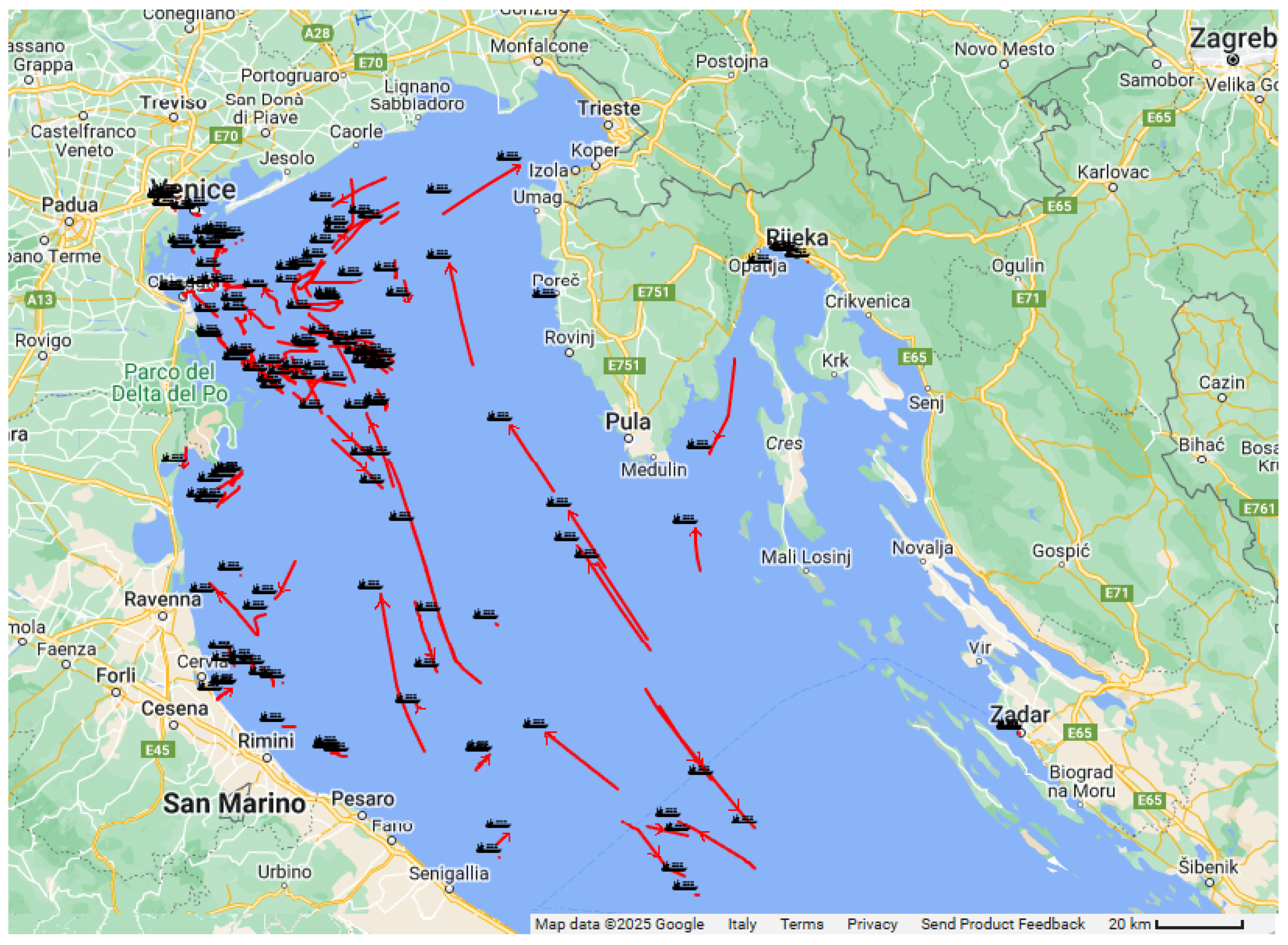
By leveraging AIS data, MNAT retrieves detailed insight into the space–time dynamics of vessel activities. To approximate a vessel’s radiated noise, the system relies on the vessel speed, location, and vessel type attributes extracted from AIS. Vessel tracking is achieved via static as well as dynamic data. The static data comprises such vessel information as its Maritime Mobile Service Identity (MMSI), vessel name, type, length, etc. Dynamic data includes position information such as longitude (LON) and latitude (LAT), as well as maneuvering data such as Speed Over Ground (SOG), Course Over Ground (COG), heading, etc. Dynamic messages are reported every 2 to 12 s, while static messages are reported every 6 min [21]. A websocket API [29] supports data streaming. Figure 2 plots the vessels’ trajectory over a time period of 90 min on a map of the Adriatic sea, between Italy, Slovenia, and Croatia, courtesy of Google Maps.
To integrate dynamic maps, geolocation services, and location-based functionalities, MNAT makes use of the Google Maps API. We support the tool with coastline border data for seas and oceans. This information is being queried from in-house databases set up for this purpose.
Finally, with an approach similar to the World Ocean Simulation System (WOSS) framework [30] we employ three oceanographic databases to retrieve data that should be provided as input to the acoustic propagation models: the World Ocean Atlas (WOA) for the SSP database (which provides sound speed profile averages on a monthly, seasonal, and annual basis from depth, temperature, and salinity observations) [31], the General Bathymetric Chart of the Oceans (GEBCO) database for ocean bathymetry data [32], and the Deck41 seabed sediment database [33].

3.2. Data Processing, Cleaning, and Imputation Pipelines

MNAT requires several ancillary processing pipelines, including AIS data preprocessing and prediction, source noise level characterization based on the vessel type, vessel trajectory prediction, sea and coastline data preprocessing, grid interpolation, real-time web interaction, storage and extraction of data in a database, and the application of underwater acoustic and ML models. For some of these methods, we introduce new approaches, whereas we apply best practices that have demonstrated good performance in the literature where possible. This section presents these methods and the results of these approaches in practice.

3.2.1. AIS Data Preprocessing

As far as vessel noise emissions estimation is concerned, AIS data regarding vessel location, trajectories, as well as vessel category is central. In particular, the vessel category is the key element to determine the noise source level, a value that also depends on speed, frequency, as well as the vessel size. For example, tankers are large vessels with comparatively slower, high-power engines that emit high-intensity, low-frequency noise. Conversely, High-Speed Crafts (HSCs) have high-speed engines that produce higher-frequency noise.
The vessel size also plays an important role in determining the intensity of hydrodynamic noise, since larger vessels displace more water and develop stronger hydrodynamic forces than smaller vessels. The draft or draught is another critical property, which refers to the maximum vertical distance between the waterline and the bottom of a vessel’s hull. Larger and heavier vessels are generally characterized by a deeper draught. Knowing the draught enables us to determine the depth of the noise source. Therefore, making accurate draft measurements is essential: the vessel depth significantly influences the estimations of vessel noise generation.
An evaluation of AIS data from online APIs [29] reveals issues with data quality including frequent errors, discrepancies, missing information, and data out of range. These issues require vast data cleaning and interpolation to correct inaccuracies. To further utilize the AIS data in MNAT, we implement a Structured Query Language (SQL) database in which different types of AIS messages are stored for further use. The Table 2 show these SQL’s tables. The International Telecommunication Union (ITU) [34] categorizes vessel types as falling under certain classes.
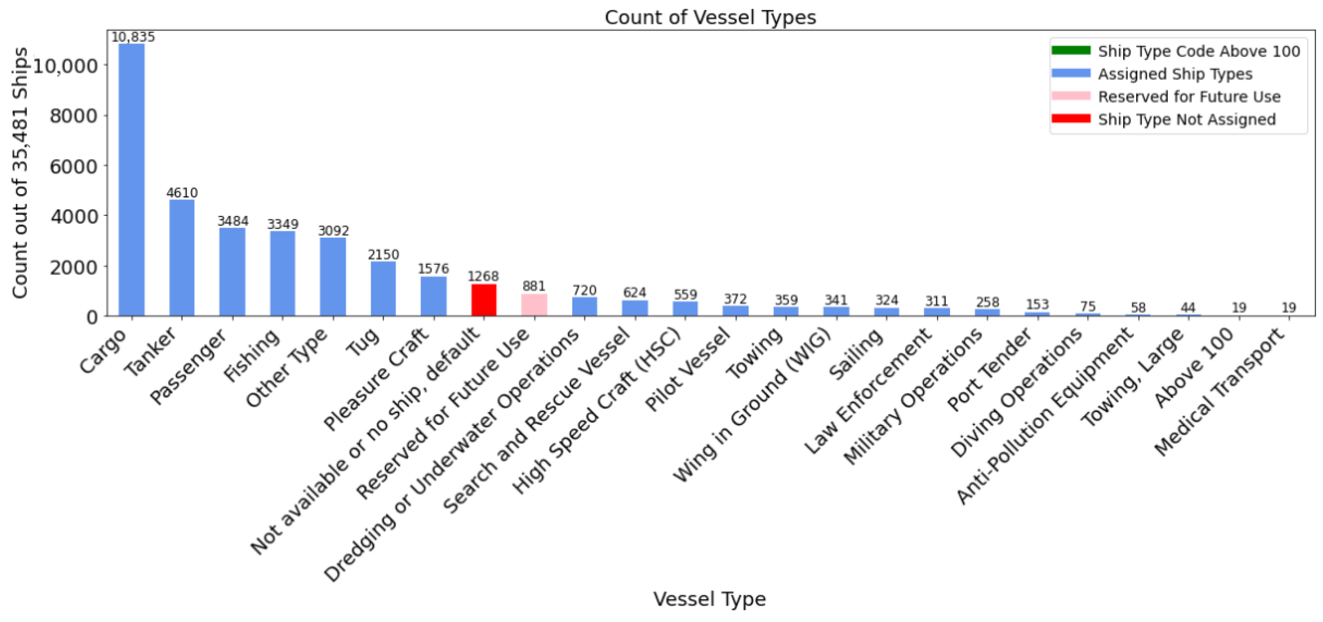
Figure 3 depicts the volume of problematic AIS data on 35,481 vessels properties and 18,240,266 vessel position reports that were collected between 2 March 2025, and 11 April 2025, across global seas. The red bars signify non-available or non-assigned ship types. Well-known AIS data providers such as (non-exhaustive list) VesselFinder, MyShipTracking, VesselTracker, and MarineTraffic primarily display raw AIS data without processing. As a result, their reports may contain unverified or inaccurate classifications.
For instance, at the time of writing this article, a vessel in an AIS report with MMSI 244615131, measuring 9 m in length and 6 m in width, was incorrectly classified as a cargo ship when, in reality, it is a tugboat. This is just one of many examples that emphasizes the need for proper data preprocessing to find anomalies and ensure accurate vessel classification.
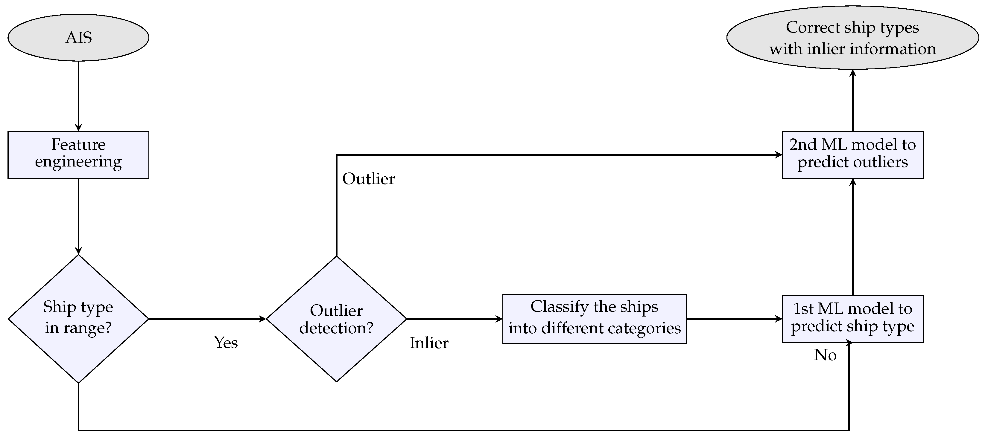
To overcome these significant AIS data anomalies and discrepancies, the algorithm depicted in Figure 4 was applied to the raw AIS data, facilitating its processing. This approach extracts reliable static, dynamic, and voyage-related information, including vessel platform shapes and navigation parameters. The pipeline employs machine learning models in order to predict vessel types and replace anomalous draft values with more realistic values.
To improve the quality of AIS data, we act on the anomalies related to the ship type, draught, and SOG values. Starting from ship-type anomalies, we first apply feature engineering on AIS information [34]. Huang [15] introduces a novel parameter called the “bridge position ratio,” which represents the ratio of the bridge’s position relative to the vessel’s length. Since most antennas or reference points are usually positioned on the bridge, this ratio can be derived from data in the AIS static message. With reference to Figure 5, which shows the bridge antenna location as a gray circle, four lengths are reported in AIS messages: A, B, C, and D. These lengths are specified by providing the distance from the AIS antenna location to the edges of the ship bow, stern, port, and starboard. The total length (L) and width (W) of the ship are calculated based on these lengths.
With the geometric and navigation measurements and parameters, the following list of new features and KPIs can be engineered:
Features = [ L , W , P r , A a , A r , C s , B p , SOG med , SOG 75 q , PerimeterToSpeed , COG med , LengthToWidth , COG 25 q , B p × A r , SogCog med , SogRange , CogRange ]
In this feature list, the static and dynamic features are defined as follows:
  • Geometric features:
    -
    L = A + B is the length of the vessel;
    -
    W = C + D is the width of the vessel;
    -
    P r = 2 ( A + B ) approximates the perimeter of the vessel;
    -
    A a = L · W approximates the area of a ship’s deck;
    -
    A r = W L indicates the overall shape of the vessel;
    -
    C s = ( L + W ) 2 L · W measures the complexity of the shape or form of a vessel;
    -
    B p = A a L quantifies the position of the vessel in terms of its total length.
  • Navigation features:
    -
    SOGmed represents the median value of the SOG, i.e., the speed of the vessel relative to the ground, measured in knots;
    -
    SOG75q represent the 75th quantiles of the SOG;
    -
    PerimeterToSpeed: P r S O G med + ϵ , where ϵ = 10 5 is a small loading factor that avoids divisions by zero;
    -
    COGmed: Represents the median of the ships’ COG, i.e., the actual direction a vessel moves over the sea, considering the impact of elements such as the wind and currents;
    -
    COG25q and COG75q represent the 25th and 75th quantiles of the COG;
    -
    SogCogmed: equals the product S O G med · C O G med ;
    -
    B p × A r : equals B p · A r ;
    -
    SpeedRatio: equals S O G 75 q S O G 25 q + 10 5 ;
    -
    LengthToWidth: L W + 10 5 ;
    -
    CogRange is Cog _ 75 q Cog _ 25 q ;
    -
    SogRange is Sog _ 75 q Sog _ 25 q .
The above features are collected from worldwide AIS data in 2025. This data includes 112,439,427 trajectory data points from ship movements and 50,283 static ship records. After some data cleaning and after removing the ships with lacking geometric information or the position record with a SOG less than 0.3, we retained data for 21,736 unique ships. These ships are categorized into eleven categories: bulk carrier, cargo, container, fishing, military, passenger, pleasure craft, research, tanker, tug, and vehicle carrier.
We use machine learning to determine the vessel type for the vessels with unknown types. To select the best machine learning model, we applied the following pipeline:
  • Data split: A three-way split is applied to data, using 60%, 20%, and 20%, respectively, for training, validation, and test sets.
  • Feature selection: From the original 17 candidate features, Recursive Feature Elimination (RFE) is applied to select the most informative features for each method.
  • Data augmentation: To address class imbalance in the training data, the Synthetic Minority Oversampling TEchnique (SMOTE) is applied on the training split only.
  • Training: Nine different methods are considered: the voting classifier [35], random forest [36], XGBoost [37], Support Vector Machine (SVM) [38], decision tree [39], K-Nearest Neighbors (KNN) [40], Gaussian Naïve Bayes (NB) [41], logistic regression, and Linear Discriminant Analysis (LDA) [42].
  • Evaluation: A comprehensive evaluation is performed using multiple complementary metrics such as accuracy and F1-score as the harmonic mean of precision and recall:
    Accuracy = T P + T N T P + T N + F P + F N
    Precision = T P T P + F P
    Recall = T P T P + F N
    F 1 - Score = 2 × Precision × Recall Precision + Recall
    where T P , T N , F P , and F N represent the number of true positives, true negatives, false positives, and false negatives, respectively.
Table 3 shows the evaluation results for the three main categories of vessels: cargo, tanker, and fishing vessels.
The table shows that the voting classifier, XGBoost, and random forest outperform the others. The ensemble voting classifier is selected because, in general, it is stable and robust as it takes several models and merges them to minimize individual errors and overfitting [43], so as to achieve better generalization. Specifically, the ensemble voting classifier combines three individual machine learning models: random forest, XGBoost, and a support vector machine that uses the Radial Basis Function (RBF) kernel.
Another major issue with the AIS data is the draught discrepancies. The draught value is essential for determining the depth of the source noise. However, Figure 6 shows the unreliability of this data. In the available AIS dataset, 6871 ships out of 35,471 (20%) report a draught value of zero. This missing data has a direct impact on transmission loss estimation accuracy and indicates source depth. To solve this problem, MNAT’s approach is to predict missing draught values using a simple linear regression model based on other vessel attributes such as length, width, and vessel type. On the other hand, some reported high draught values (e.g., 50 m) are deemed invalid for a ship’s normal physical dimensions.
A typical outlier case is when the AIS-reported draught is bigger than this minimum bathymetry depth. One solution to correct such outliers is then to substitute the draught value with the shallowest ocean bottom depth along the entire navigational route of each vessel.
The next type of anomaly to be compensated for is the SOG anomaly. SOG is a key parameter in determining the noise level at the ship location. Equation (1), presented in [44], defines the relationship between the ship’s SL and its SOG:
SL = S L 0 + C v × log 10 S O G v r
where C v is the velocity coefficient and is defined as the SL variation for per order of magnitude of variation of the speed; v r is the reference velocity (equal to 1 knot), so that the logarithm’s argument becomes dimensionless; and S L 0 represents the estimated source level at the reference speed.
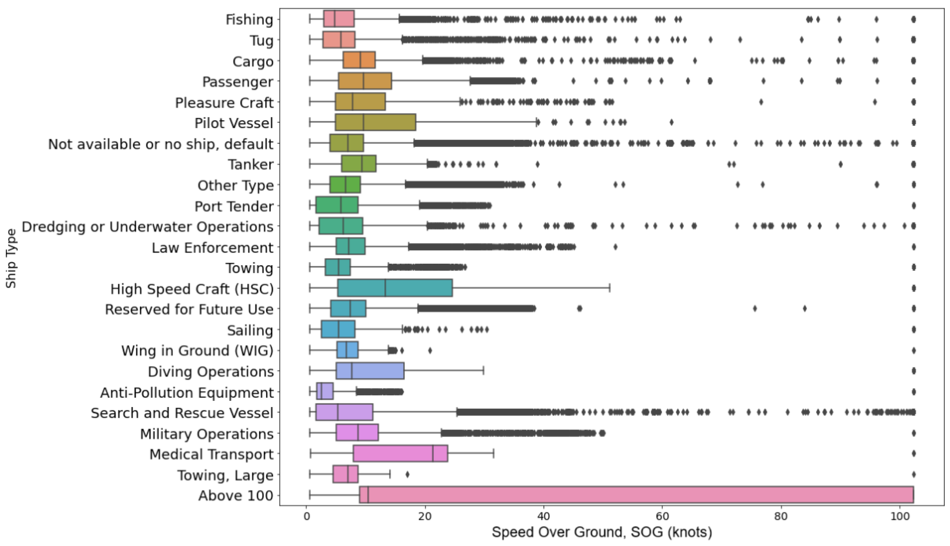
Figure 7 illustrates the anomalies found in the processing of SOG data for different ship classes via bar plots. For example, in AIS records, cargo, tanker, or tug vessels are reported to be traveling at up to 100 knots, or ≈185 km/h (for reference, 1 knot corresponds to ≈1852 km/h). Such values are at odds with the operational characteristics of these types of vessels and are physically unrealistic.

3.2.2. Finding Source Noise Levels

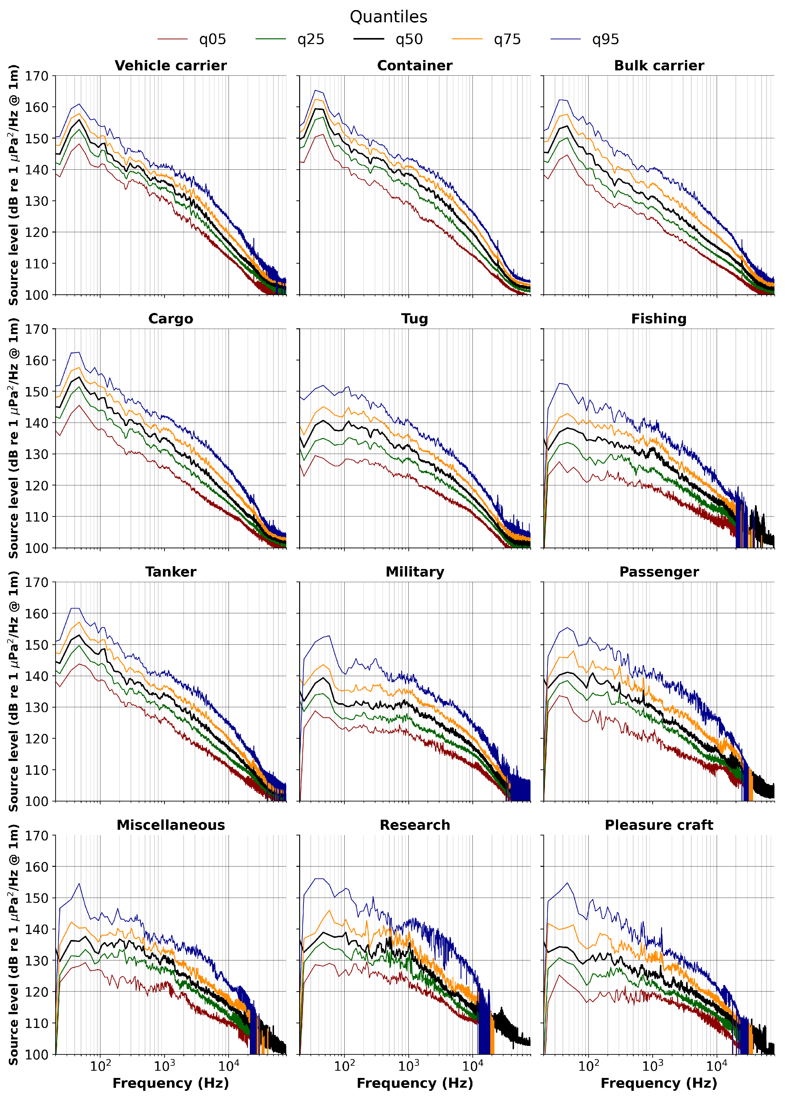
In the previous step, the correct vessel type was determined to estimate the approximate noise source level in dB re 1 μPa. Several methodologies have been proposed to model vessel-generated noise. For example, in the NAVISON project [7], Underwater Radiated Noise (URN) emissions from vessels are computed using PIANO [45]. PIANO utilizes ship design and operational parameters to separately estimate contributions from cavitation and mechanical noise to the vessel URN. However, this method relies on parameters that are often unknown and difficult to retrieve (e.g., the specific propeller model, the engine stroke type, and other physical engine features [28] that are typically not included in public AIS transmissions). In this project, we use real data of the noise spectrum levels from 2809 isolated vessels. These vessels commuted near the shoreline in the Haro Strait (WA, USA) and were measured by Veirs [46]. By extracting the data and calculating the noise levels across different frequencies, the noise levels were classified into 12 ship types. Figure 8 illustrates the median noise level for each vessel type.
Since vessels within each category are also scaled based on size, and size plays a significant role in generating noise, for each category, a regression function is applied to estimate the noise level based on AIS characteristics. Figure 9 displays the quantile ranges (5th, 25th, 50th, 75th, and 95th percentiles) of the noise levels for all classes of vessels.

3.2.3. Vessel Trajectory Prediction Using AIS Data

AIS reporting intervals may vary depending on a vessel’s speed, rate of turn, and navigational status. However, it can also occur that an AIS message cannot be sent within the specified reporting interval, perhaps due to a lack of time slots, skipped messages, or losses during VHF transmission. Then, due to timeouts, the vessel can disappear from the AIS systems [47]. A vessel trajectory prediction algorithm can help fill the information gaps when we need to estimate the noise radiation from a given vessels’ position. Having an updated position for each vessel in the area where noise estimation is sought is necessary in order to make sure that the estimate is accurate.
For this purpose, MNAT is complemented with TrAISformer [48], a deep learning model for vessel trajectory prediction using AIS data. We applied TrAISformer to the AIS dataset we retrieved from the API, which contains 18,240,266 positioning messages collected from vessels of various types across global waters over a 40-day period, from 2 March 2025 to 11 April 2025. TrAISformer uses a high-dimensional sparse representation of AIS data and a probabilistic transformer architecture to account for long-term dependencies and achieves state-of-the-art accuracy in vessel trajectory prediction tasks, with a 2 h-ahead error of 0.94 nautical miles (41% better than its immediate competitor GeoTrackNet [48]).
As described by Nguyen et al. [48], TrAISformer also performs significantly better than state-of-the-art deep learning models like LSTM seq2seq, Conv seq2seq, GeoTrackNet, and attention models. It produces much smaller mean prediction errors of 0.48, 0.94, and 1.64 nautical miles for 1 h, 2 h, and 3 h lookahead times, respectively. We resorted to a transformer model rather than to multi-layer perceptrons or other neural architectures because they have been observed to be outperformed by transformers [48].
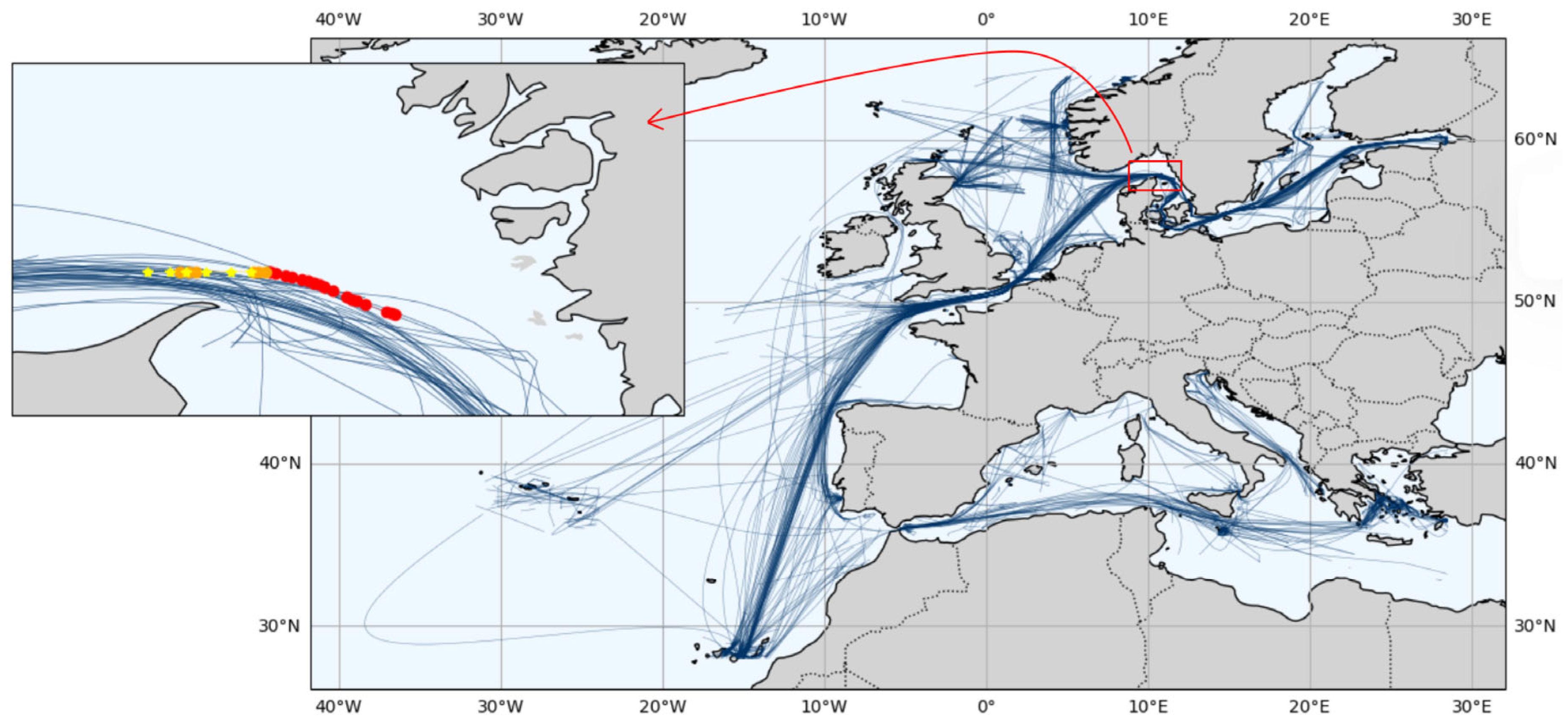
Figure 10 shows AIS-based vessel trajectories across Europe, along with an example of vessel path prediction between the Skagerrak and Kattegat, located north of Denmark. We observe that this prediction technique has a low degree of discrepancy and can follow the distinctive navigation patterns around landmasses and coastal passages because it takes into account vessel type information and is trained on historical trajectory data.

3.3. Noise Prediction Using Machine Learning Models

Once vessel data in a given ocean area have been collected and corrected if needed, and once the location of all vessels has been estimated, it becomes possible to run acoustic propagation models to compute propagation losses and ultimately retrieve the noise intensity at any point in the area.
However, running the Bellhop or RAM acoustic models is a resource-intensive process, especially when large sea bodies and long distances are considered. For example, on a modern laptop, estimating the noise between two points that are 320 km apart takes around 18 to 20 s, using the Bellhop software with 50 intermediate bathymetry points and a maximum depth of 230 m. With this depth, the WOA database returns 11 SSP values for each intermediate point. As a result, for a ship as a source of noise with 60 selected points on the coastline, the total estimation time might exceed one minute. Scaling this process to 100 ships would significantly increase the computational time. To complement these precise but slow acoustic models, we propose a faster approximate approach.
Specifically, we train a machine learning model using data previously estimated by RAM or Bellhop. This ML model can estimate noise from other sources, including those that were not processed by the acoustic model or those ships that have moved to new locations. Then, for the entire sea area, we always have an up-to-date total noise level. The system ingests additional data in a continual learning fashion and becomes more accurate as more data is processed. From the available data, we engineer the following features for the target variable (value):
Features = Latitude Source , Longitude Source , Latitude Grid , Longitude Grid , Distance Source Grid , Distance Source Grid 2 , LoS Source Grid , Bearing Source Grid
Using data from four ships (1574 grid points per ship, totaling 6296 points) in the Adriatic sea and the above feature structure, training, validation, and test data sets are created with a 60%, 20%, and 20% split, respectively. The small number of four ships was selected to show that the ML model output is already acceptable when little data from just a few ship is available, and improves its accuracy significantly by adding data from additional ships. We compared several regression models to predict noise levels based on their ability to capture the underlying patterns in the data. A variety of ensemble and single-model approaches are tested for this noise prediction. The performance of these different methods is listed in Table 4.
The Stacking Regressor (SR) worked effectively in resolving noise forecasting with high precision and reliability, as evaluated in terms of Mean Absolute Error (MAE), defined as the average of the absolute differences between predicted values and true values
MAE = 1 n i = 1 n y i y ^ i ,
of Root Mean Squared Error (RMSE), defined as the square root of the average of the squared differences between predictions and true values
RMSE = 1 n i = 1 n y i y ^ i 2
and of the R-squared value
R 2 = 1 i = 1 n y i y ^ i 2 i = 1 n y i y ¯ 2 ,
where y i is the observed value, y ^ i is the predicted value, y ¯ is the mean of observed values, and n is the number of observations. The R 2 value represents the proportion of variance in the true values explained by the model’s predictions. R 2 1 indicates a near-perfect fit, R 2 0 indicates that the model performs no better than predicting the mean, and R 2 values less than 0 mean that the model is worse than predicting the mean.
In this system, the SR outperforms by achieving a 2.6 MAE (dB re 1 μPa), 3.2 RMSE (dB re 1 μPa), and an R 2 value of 0.98. Stacking regression elicits strengths in a combination of a variety of base models by learning ways in which these models’ predictions can be aggregated. Stacking regression is structured as follows:
A.
Base Models:
  • Extra trees regressor: A robust ensemble method that builds multiple decision trees to reduce the variance of the noise predictions.
  • XGBoost regressor [37]: A gradient boosting algorithm that efficiently handles complex patterns in data.
  • LightGBM regressor [49]: A gradient boosting framework optimized for speed and efficiency.
  • CatBoost regressor [50]: A gradient boosting model that performs well with categorical features and avoids over-fitting.
B.
Final Estimator: A ridge regression [51] model was used as the meta-model to combine the outputs of the base models.
The stacking model was trained with a 5-fold cross-validation to ensure generalization and robustness. Each model in the Table 4, apart from the MAE, RMSE, and R 2 evaluation metrics values, has unique advantages and limitations when it comes to underwater noise prediction in MNAT. Although XGBoost and LightGBM are sensitive to overfitting, they are powerful in capturing nonlinear relations. CatBoost needs large and well-balanced datasets to maintain consistent accuracy. Although Random Forest and Extra Trees produce higher variance close to complex coastlines and tend to underfit fine acoustic variations, they offer robustness against inconsistencies and uncertainties in the training data. Gradient Boosting suffers from slow training and a heavy reliance on hyperparameter tuning. While the voting regressor increases stability through averaging, it is unable to model nonlinear dependencies among regressors. KNN is sensitive to sparse and high-dimensional spatial data, and thus yields the worst performance among the tested methods. Conversely, the Stacking Regressor effectively overcomes the above constraints by leveraging the complementary strengths of all base models.
In the following Section 3.3.1 and Section 3.3.2, we explain how we provide a training dataset for the stacking model.

3.3.1. Vessel Clustering and Scoring via a Gaussian Mixture Model

As expected, the choice of the vessel noise maps used for training affects the quality of the interpolation output. In particular, training data should be representative of different source locations in order to yield a robust result that remains accurate for different ship locations.
We recall that MNAT can start using machine learning for noise map regression after the noise maps of representative vessels have been obtained from propagation models (Bellhop or RAM). In order to select such representative vessel noise maps, in MNAT we deploy an automatic clustering method based on a Gaussian Mixture Model (GMM) [52,53] to find representative vessel clusters based on 40 days of AIS data, from 2 March 2025 to 11 April 2025. Because each sea basin has different characteristics (e.g., in terms of shore shape and bathymetry), we deploy a different GMM model for each sea, where each model has a different number of identified clusters C . Clusters are determined by training on the above 40-day AIS data trace.
Once the clusters have been determined, the GMM parameters of each cluster c are characterized by their cluster centroid coordinates μ c R 2 , by the covariance matrix Σ c R 2 × 2 describing the spatial spread and orientation of the cluster, and by the cluster weight (prior probability) π c ( 0 , 1 ) , representing the prevalence of the cluster in the dataset, with c = 1 C π c = 1 .
When running MNAT, the system starts streaming AIS data and computing the noise maps due to the vessels found. Having the GMM cluster characteristics, we are now in a position to determine which vessels should be used to train the noise map’s stacking regressor using a scoring system. Assume MNAT identified vessels { v 1 , , v m } from the AIS data, where v i R 2 denotes the coordinates of vessel i. We assign a score to each vessel as follows. We recall that the probability density function of the GMM is as follows:
p ( v ) = c = 1 C π c N ( v μ c , Σ c ) ,
where v is the location of a vessel, and N ( v μ c , Σ c ) represents the Gaussian distribution having parameters μ c and Σ c , evaluated at location v . We first compute how strongly the vessel at v is connected to cluster c as
L c ( v ) = log N ( v μ c , Σ c )
and weigh this metric by the prior π c and a parameter β to yield
s c = L c ( v ) + β × log π c .
Here, β determines whether the scoring treats all clusters equally by β < 1, favors bigger and more frequent clusters by β > 1, or weighs them by the same prior π c if β = 1. We then apply the softmax function to the scores
p c = exp ( s c ) j = 1 C exp ( s j ) .
Finally, we take the cluster yielding the maximum score, c * = arg max c s c , and compute the final vessel score as
Score = s c * + α × p c * ,
where α is a normalization factor chosen to yield score values up to 100, while rebalancing the weight of the confidence p c * against s c * .
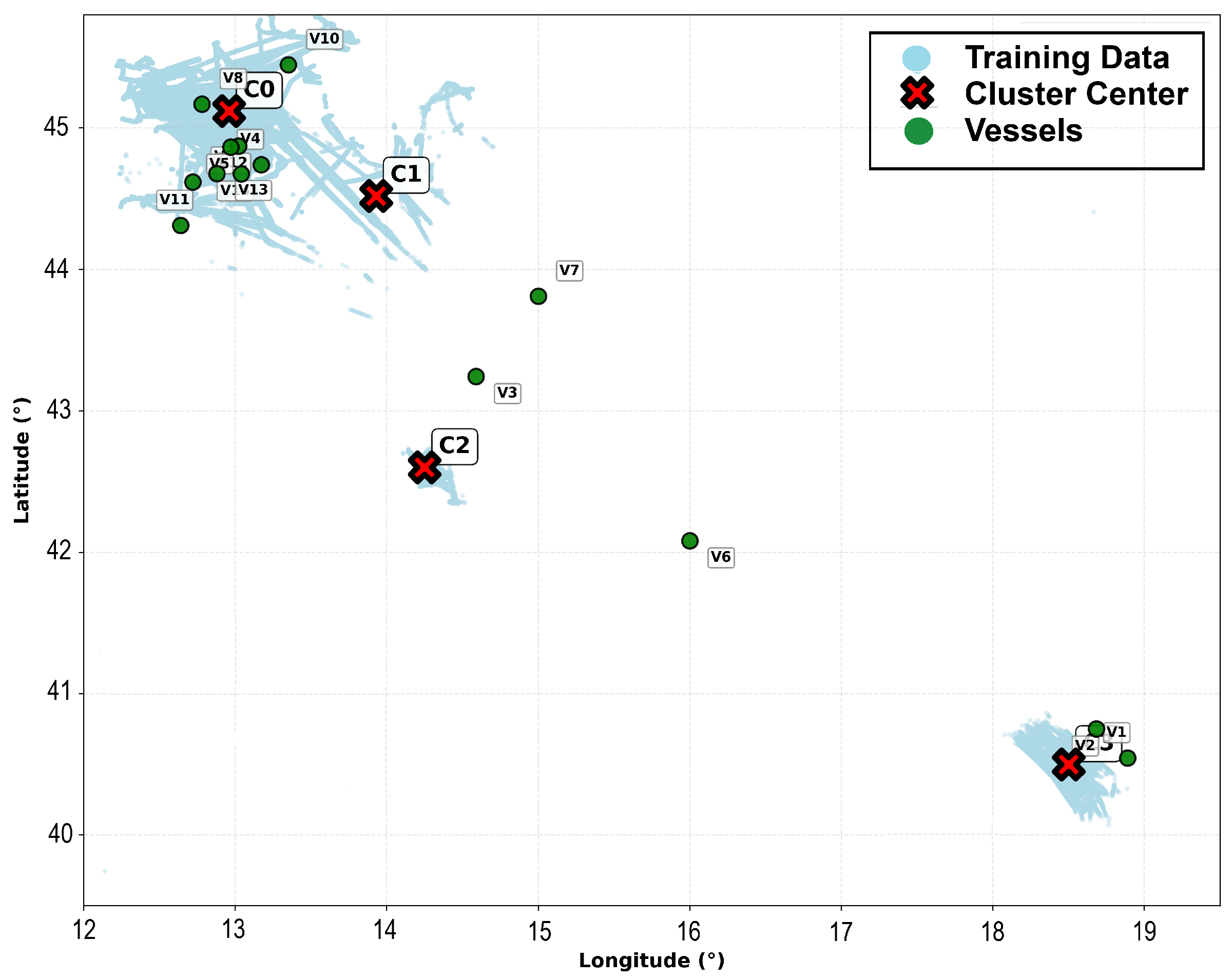
Table 5 presents the clustering and scoring results for a list of 14 vessels reported by AIS in the Adriatic sea. The distribution of this AIS-reported vessel (green points) is displayed in Figure 11. Light blue points in the background represent the raw dataset that was used to train the GMM. Four cluster centers have been identified in this area and are are denoted as bold red crosses.

3.3.2. Sorting Vessels for Training the Stacking Regressor

After having computed the scores of each vessel, MNAT picks the vessel with the highest score for each cluster of the GMM and includes its modeled noise map in the training set. Then it adds extra vessels based on each cluster’s prevalence as follows. For each cluster c = 1 , , C , MNAT computes the ratio i c / q c between the number of vessels already included in the dataset and the number of vessels in the cluster. Then it adds one ship to the dataset from the cluster for which the ratio is minimum. For the scenario depicted in Figure 11, the ordered list of vessels used for training is reported in Table 6.
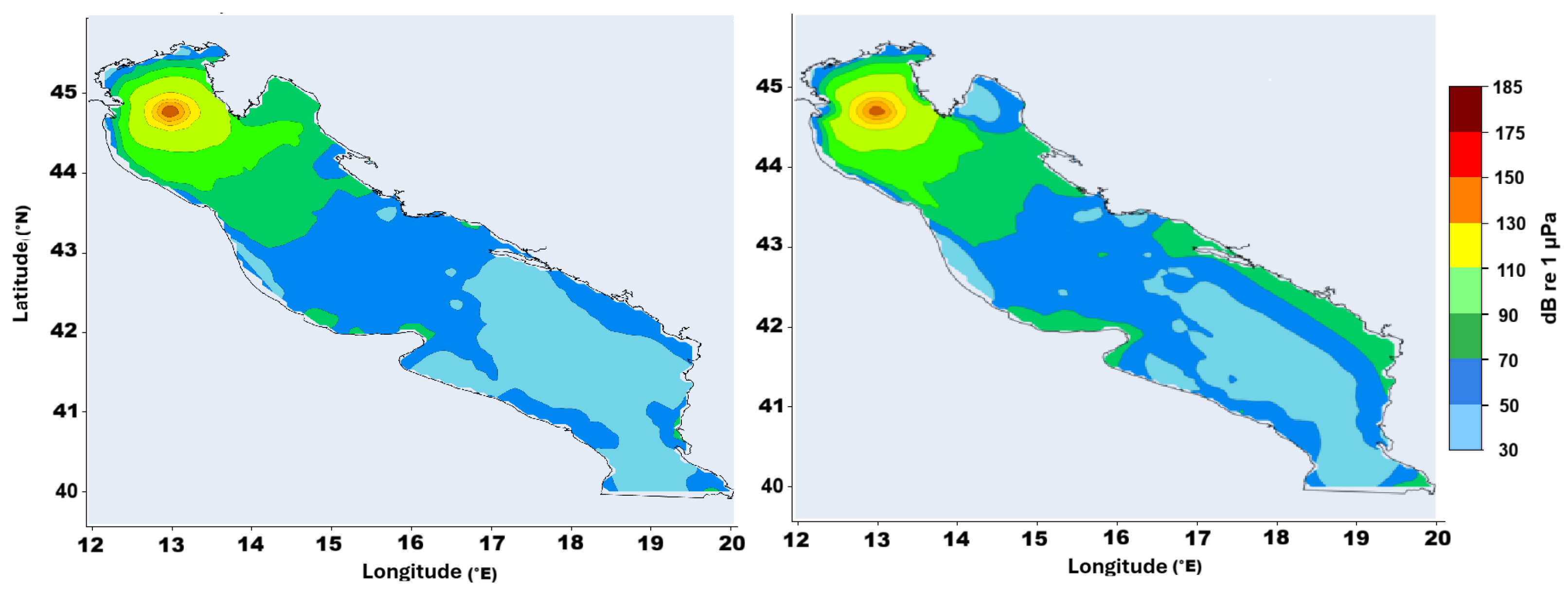
Finally, the stacking regression model in MNAT was designed to generalize across geographically diverse marine environments by combining Bellhop/RAM modeling with data-driven learning. To ensure regional adaptability, MNAT groups vessels and spatial distributions using a clustering framework based on GMM for each sea basin. Figure 12 displays the result of SR noise prediction for a ship in the north of the Adriatic sea. The left side illustrates the predicted noise from the stacking regressor model, while the right side shows the estimated noise from the acoustic model. The SR predictions are acceptable because, for this ship location, more than 85% of the noise samples are correctly predicted. This prediction contributes to the overall noise map of the sea, which includes combining with the other ships’ SR predictions and Bellhop/RAM estimations. As the process progresses, these SR data will be replaced by acoustic model estimation data in the subsequent stages.

3.3.3. Sea and Coastline Data Preprocessing

Shoreline identification is an essential step to enhance the precision of noise propagation modeling in marine environments. This entails two crucial steps: identifying tiny islands and obstructions that could affect acoustic propagation, and choosing the best near-shore points up to which noise estimation should extend, in order to increase the computational efficiency.
To identify islands and underwater obstacles that affect the propagation models in a given maritime region, bathymetric data at the highest resolution available in the GEBCO bathymetric dataset is used. A binary land–water mask is created from bathymetric data for further analysis. We identify landmasses, including islands and barriers, by using OpenCV to extract contours from the binary land–water mask. Islands inside aquatic bodies are discovered independently via nested contour reconstruction. To make additional analysis easier, the centroid, bounding box, and area of each discovered landmass is calculated.
As an example, Figure 13 shows the obstacles and islands detected in the Sulu archipelago, in the southwestern area of the Philippines.
Finally, a dataset for all detected obstacles and islands is created, which includes the following attributes:
[ ID , Centroid X , Centroid Y , Centroid Longitude Centroid Latitude , Area , BBox X , BBox Y , BBox Width , BBox Height
The meaning of the feature elements is as follows:
  • ID: A unique identifier assigned to each detected obstacle or island.
  • CentroidX: The X-coordinate (cartesian) of the object’s center in image space.
  • CentroidY: The Y-coordinate (cartesian) of the object’s center in image space.
  • CentroidLongitude: The geographic longitude of the object’s centroid.
  • CentroidLatitude: The geographic latitude of the object’s centroid.
  • Area: The surface area of the object in pixels or grid cells.
  • BBoxX: The X-coordinate of the top-left corner of the object’s bounding box.
  • BBoxY: The Y-coordinate of the top-left corner of the object’s bounding box.
  • BBoxWidth: The horizontal size of the bounding box in pixels.
  • BBoxHeight: The vertical size of the bounding box in pixels.
To choose the optimum coastline points for the computation of noise along the coast, the following procedure is applied. In marine environments, coastline data often consists of a large number of points. For example, available coastline data for the Adriatic sea consists of 48,000 points, making it impractical to apply acoustic models for all points. We thus select a limited number of optimum points along the coastline based on a predefined threshold, which controls the resolution of point selection.
The first point in the dataset is chosen as the beginning reference point (pref) at the start of the operation. The algorithm then determines the distance Destnorm(pref) between this reference point and the source of the noise. The “norm” subscript conveys that the metric is normalized by the difference between the maximum and minimum distances of the ship to the coast, in order to adapt the metric to different seas having different surface areas. The cumulative angular sweep, or Arc(k), is then updated step by step, by calculating the Arc (bearing angle) formed between the current location, the vessel, and the next coastal point in sequence. Therefore, we define the Geometric Factor (GF) to be used in the optimum points selection process:
G F ( p ) = Dest norm ( p ref ) · k = p ref p Arc ( k ) 2
If G F ( p ) exceeds a user-tunable coastline representation accuracy, the current reference point is replaced by the most recent point for which azimuth was calculated. This newly selected point is then added to the set of optimal coastline points.
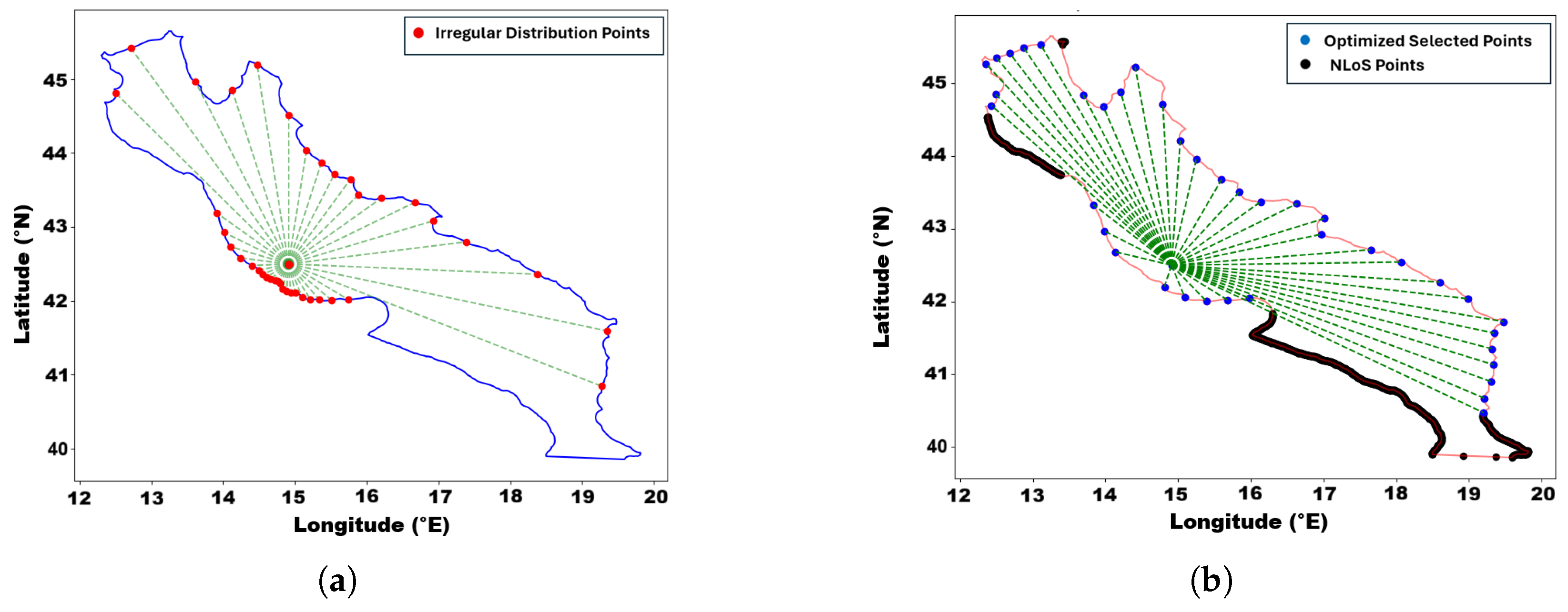
Figure 14 shows the resulting optimal point set after applying the above approach along the coast of the Adriatic sea. This number of coastline points has been calculated by Equation (10) when we set the threshold to 15; it is obvious that when we increase the threshold, the distance between two consecutive points will increase. In panel (a), 40 points are irregularly distributed, as one coastline point is picked every 360 ° / 40 = 9 ° . As a result, there exist regions of sparse as well as highly dense distributions of points. In contrast, plot (b) reflects a far more uniform scattering of those 40 points, ensuring better coverage of the Adriatic sea’s coastline. Additionally, in the optimized coastline selection method, the Non-Line-of-Sight (NLoS) points from the ship location are excluded from calculations. Black lines in Figure 14 depict these NLoS regions.

3.3.4. Radial Sampling Strategy

In order to estimate the radiated noise intensity over a given sea basin, one method is to compute the noise propagated from each source (e.g., each vessel) up to a set of points uniformly distributed throughout the area. A natural choice would then be to arrange these points into a regular grid. However, this is not the optimal choice from the point of view of the calculations required by acoustic propagation models. These models solve differential equations over space and time using numerical methods, and the best choice is thus to reuse such calculations as much as possible. In the case of Bellhop, for instance, it is much more convenient to find sound ray trajectories and sound pressure once for a set of points distributed along the range dimension of a vertical ocean slice starting from a fan of emitted rays, rather than repeating such calculations separately for a number of non-aligned points.
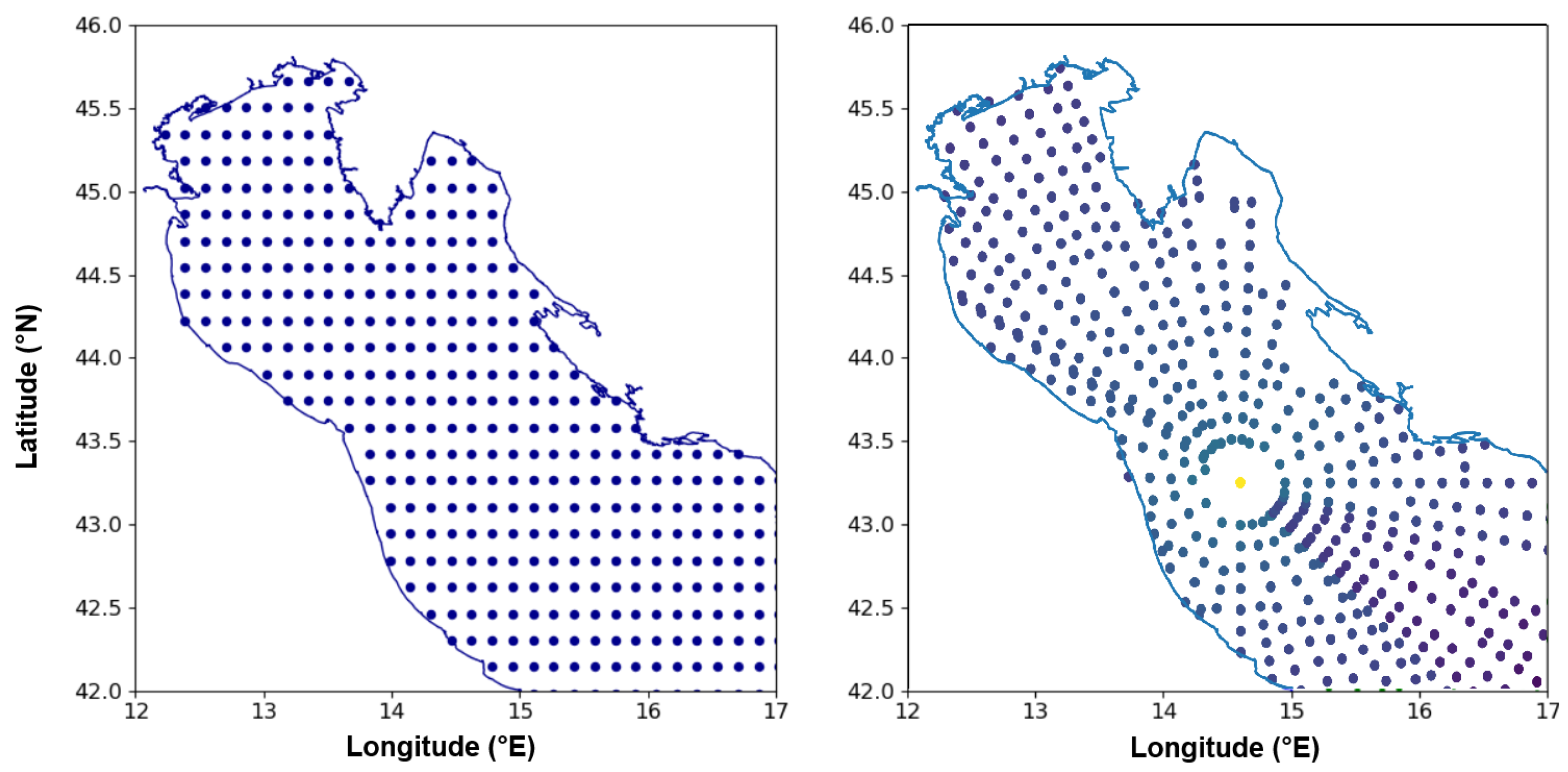
With the above rationale in mind, the optimum set of shoreline points is identified via the method in Section 3.3.3, and their locations are used as the endpoints of the fans of a circular grid centered on the noise source. Using a circular grid translates into a much more efficient computation process. Figure 15 shows the difference between these two methods for a part of the Adriatic sea.

3.3.5. Grid Data Imputation

Even though computing the sound pressure over a circular grid leads to a more efficient process, the representation of data for user visualization (e.g., in the form of a noise heatmap superimposed on a geographical map) still requires a regular rectangular grid. We then investigated the best method to impute radiated noise intensity values in a regular grid, starting from the values computed in the circular grid. Specifically, the following methods are implemented and evaluated:
  • Datagrid (Nearest neighbor): Ref. [54] utilizes the closest known point without regard to surrounding variability.
  • Datagrid (Linear): Ref. [55] estimates between neighboring data points in a triangle.
  • CloughTocher: Ref. [56] a piecewise cubic interpolation method on triangulated irregular networks that produces smooth and continuous surfaces.
  • RBF: Ref. [57] uses radial basis functions centered on data points in constructing a smooth surface.
  • Inverse Distance Weighting (IDW): Ref. [58] a deterministic method in which unknowns are approximated by a weighted average of nearby observations, where the weights are inversely related to distance.
  • Ordinary kriging: Ref. [59] a geostatistical technique that utilizes variograms to account for autocorrelation while making minimum-variance, unbiased predictions.
  • Gaussian Process Regression (GPR)-Physics: Ref. [60] an advanced interpolation technique that models spatial correlations in oceanographic data using Gaussian process regression. It automatically learns the best parameters (such as measurement noise levels and spatial correlation length scales) from the training data. The technique uses a WhiteKernel, which explicitly models the noise in GPR to find and remove it, and uses the RBF kernel to make the interpolation smooth and continuous [61]. In addition to interpolated values, GPR-Physics also provides uncertainty estimates (standard deviations) for every grid point during prediction. This distinguishes GPR-Physics from other interpolation techniques by measuring prediction confidence while preserving physics-aware spatial modeling.
  • Ensemble MultiMethods Physics: the goal of this physics-based ensemble approach is to produce more reliable results than any one method could by combining IDW (60%), ordinary kriging (20%), and RBF (20%) interpolation techniques. Furthermore, it uses the Euclidean distance to determine the closest interpolated value for each grid point. Then, compute a weighted average in which IDW is used for local accuracy and other methods are used for global spatial correlation. In the integration of physics step, it makes use of real geographic coordinates (latitude/longitude) and takes spatial relationships between points into account.
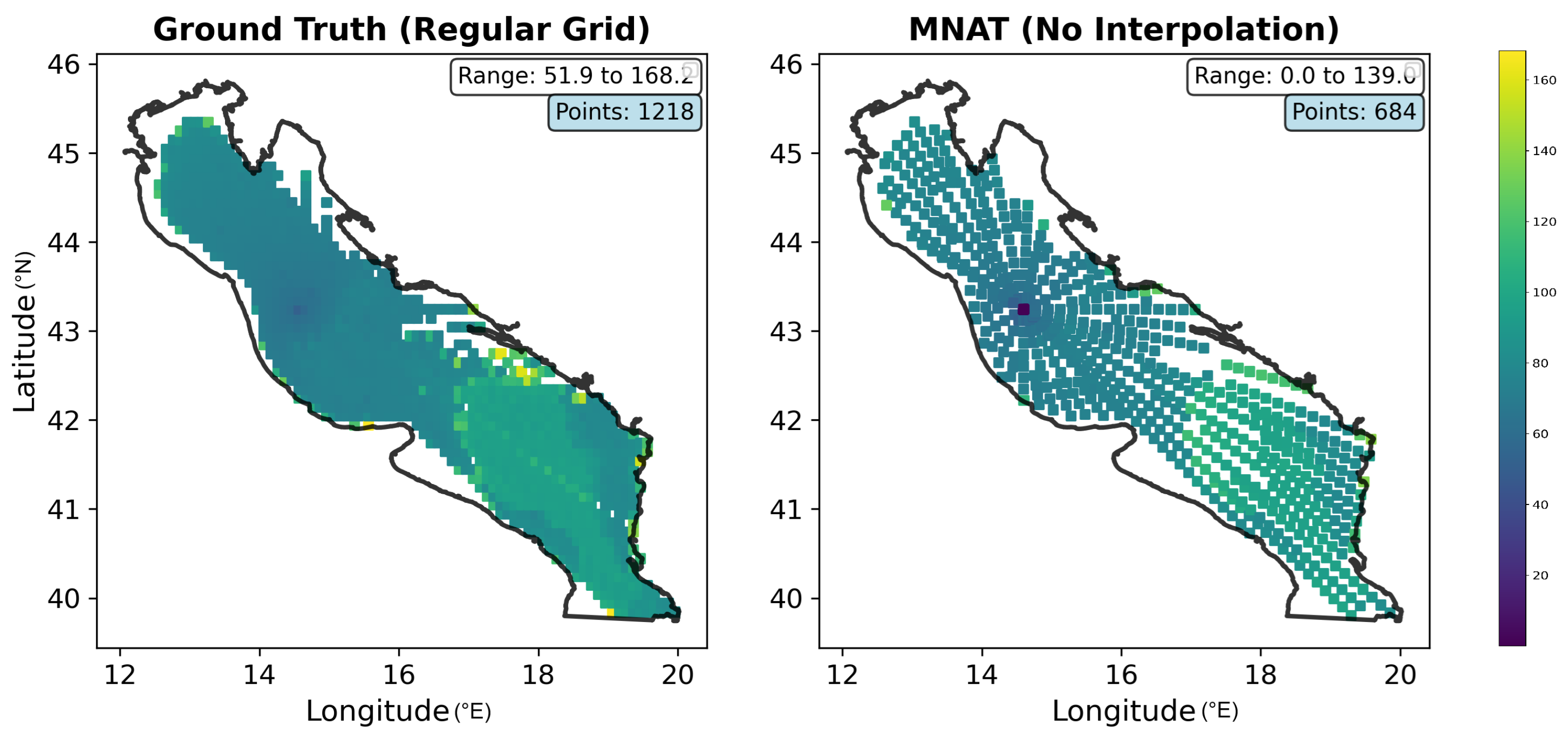
Figure 16 shows the ground truth data obtained by applying the Bellhop models separately for a ship located at ( 43.24 ° N , 14.59 ° E ) and all 1574 regular grid points on the Adriatic sea, on the left, which is used as a reference to evaluate the different interpolation methods. The panel on the right presents the result of the Bellhop model estimation for this ship as a source of noise and selected points on the coastline.
In Figure 16 we have the regions that are not filled by Transmission Loss (TL) estimation. This occurs because certain areas are not in line-of-sight of the source, or some of them are shallow-water estimates from a deep-water source.
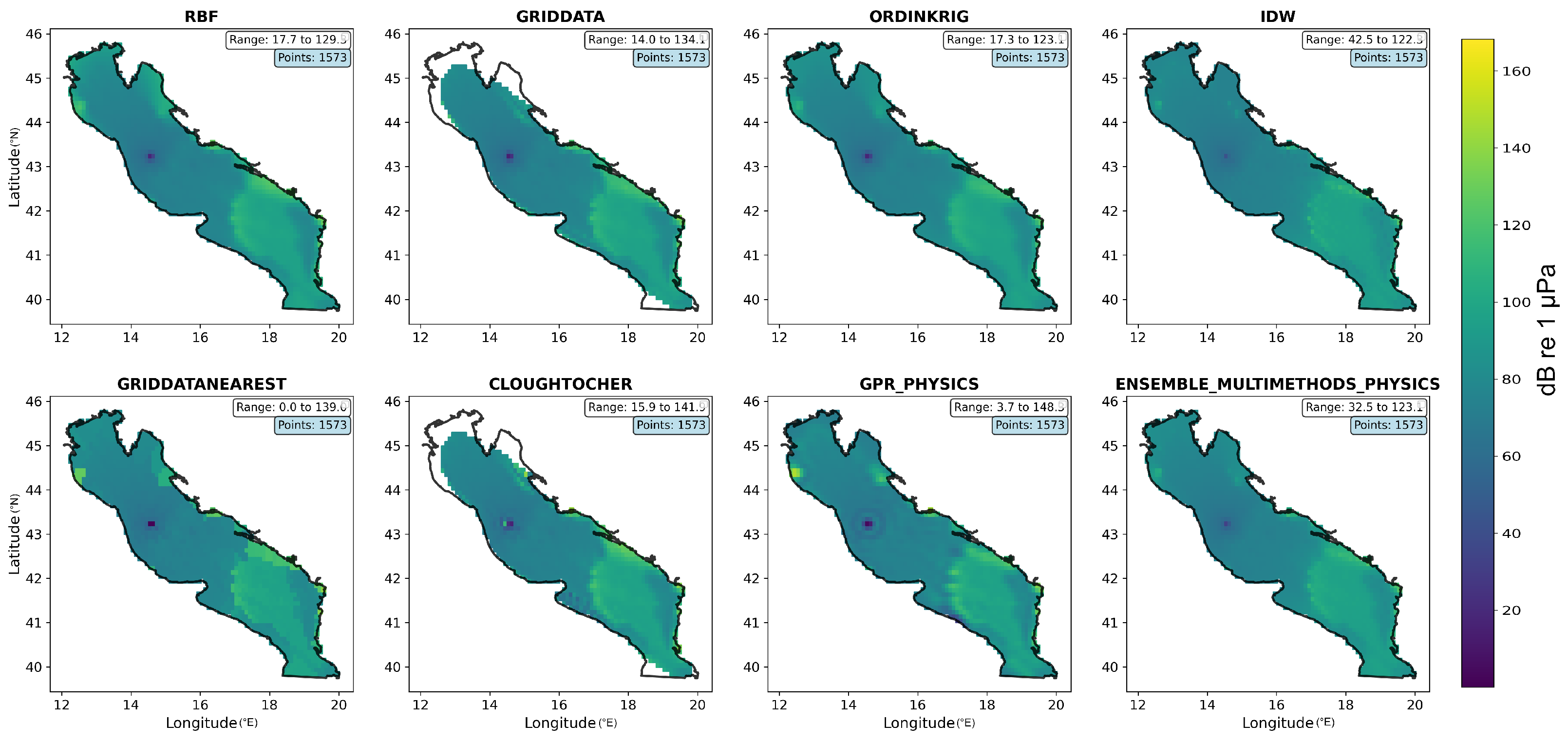
Figure 17 shows the results yielded by the aforementioned interpolation methods. In the griddata (linear) and CloughTocher methods, the areas near the coastline are not filled by interpolated data. These two methods rely on Delaunay triangulation of the input points, which only defines interpolation inside the convex hull of the data points. Then the points outside cannot be interpolated. In this case, some coastline points fall outside the convex hull, leaving gaps. This issue can be fixed by adding extra regular grid points, at the expense of extra computational costs.
To achieve the best results, we tuned the hyperparameters for the aforementioned interpolation methods. Table 7 shows the most important tuned hyperparameters for these interpolation methods.
All these observations, tunings, and evaluations are further confirmed by the error maps in Figure 18, which illustrate the deviation between each interpolation method and the ground truth noise map derived from modeled noise propagation maps.
Based on MAE and RMSE evaluation metrics, the IDW [62] method performs better overall. In particular, IDW outperforms in the vicinity of the noise location. The ship is in (43.24, 14.59), and all methods’ deviation is high around this location except IDW.

3.3.6. Google Maps Integration for Noise Mapping

The computed underwater noise distribution is displayed with a web-based interface that also plots ship trajectories with interactive mapping functionality similar to Google Maps. The heatmap is generated using a static grid where each point represents cumulative noise levels from all AIS-reported vessels. The noise at these points is calculated via either RAM or Bellhop models, as well as interpolation.
The results and real-time information, such as AIS data, and the list of islands and obstacles in sea areas after cleaning and preprocessing are stored in in-house databases for future analytics, investigations, or predictive purposes.

4. Use Cases

MNAT is designed to analyze propagated noise in marine environments, not just from vessels, but potentially from any source or set of sources. In order to showcase two such different scenarios, we now discuss two use cases.

4.1. Vessel Noise Propagation

The primary use case of this tool is modeling and analyzing vessel noise propagation in marine environments. It evaluates underwater noise spread by simulating the radiated noise of vessels with various sizes and operating conditions. As already mentioned, showing the real-time propagated noise in any sea worldwide is the main feature of MNAT when the user selects a specific sea from the list.
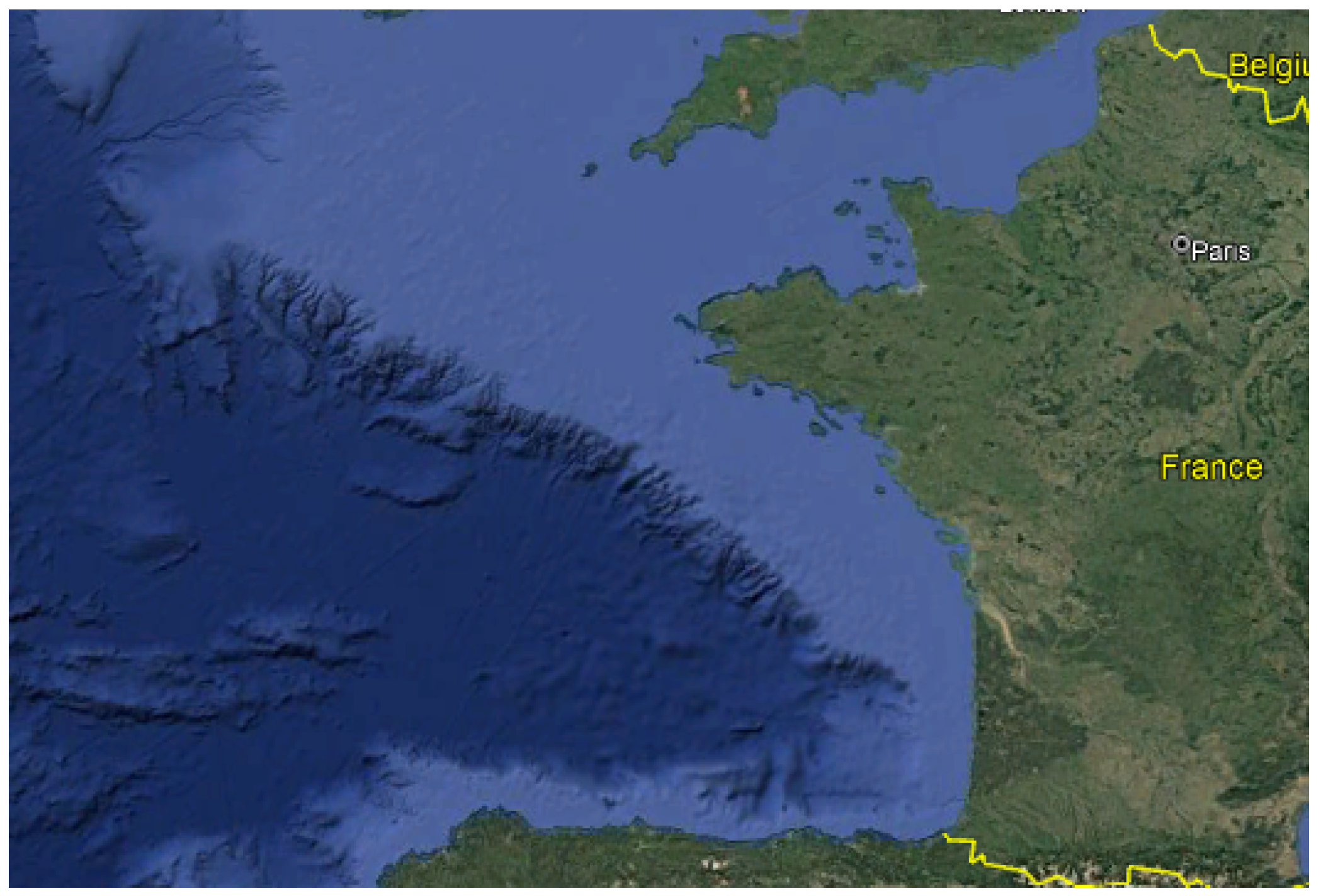
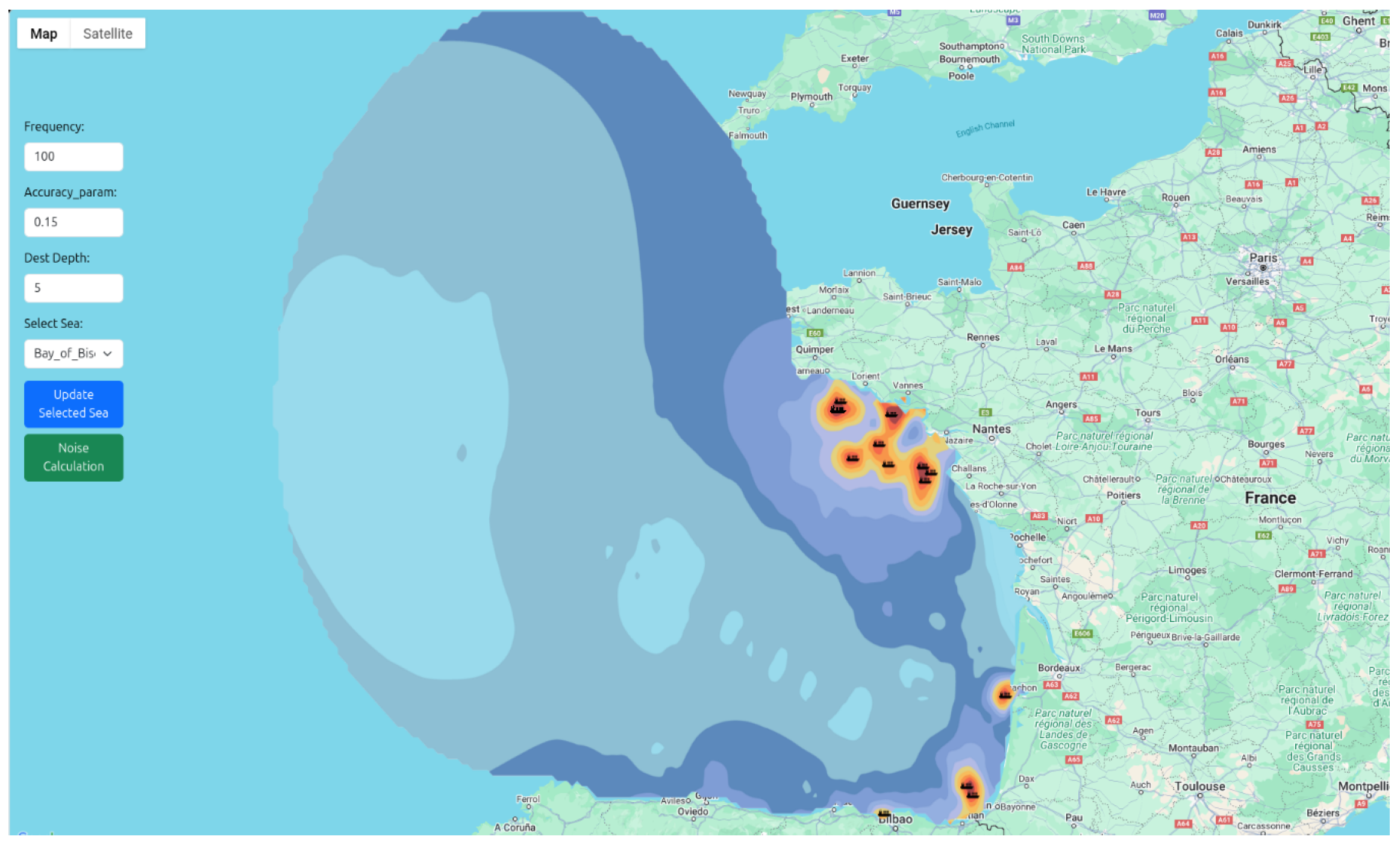
For example, consider the Bay of Biscay, between the western coast of France and the northern coast of Spain, at 3 a.m. on 6 May 2025. The Google Earth plot in Figure 19 shows the bathymetry of the area. Figure 20 shows the generated noise of ships in the Bay of Biscay, where the greatest concentration of noise from shipping activities is around the northern area of France (from Nantes up until Quimper in the Brittany region), near the Port of Arcachon (Bordeaux area), in the cross-border area of San Sebastian/Bayonne, and near Bilbao, Spain. From the MNAT output in Figure 20, the noise produced by such ships is shown to propagate well into the continental shelf area and to affect the deeper oceanic regions comparatively less. Here, dark red hues represent high noise, whereas yellow, dark blue, and light blue hues convey progressively lower noise levels. The bathymetry of the area and the presence of islands (e.g., the Île d’Yeu, off the coast of Challans, France) protects other ports to the south, such as La Rochelle and Royan, from being directly affected by the noise that propagates from the northern areas.
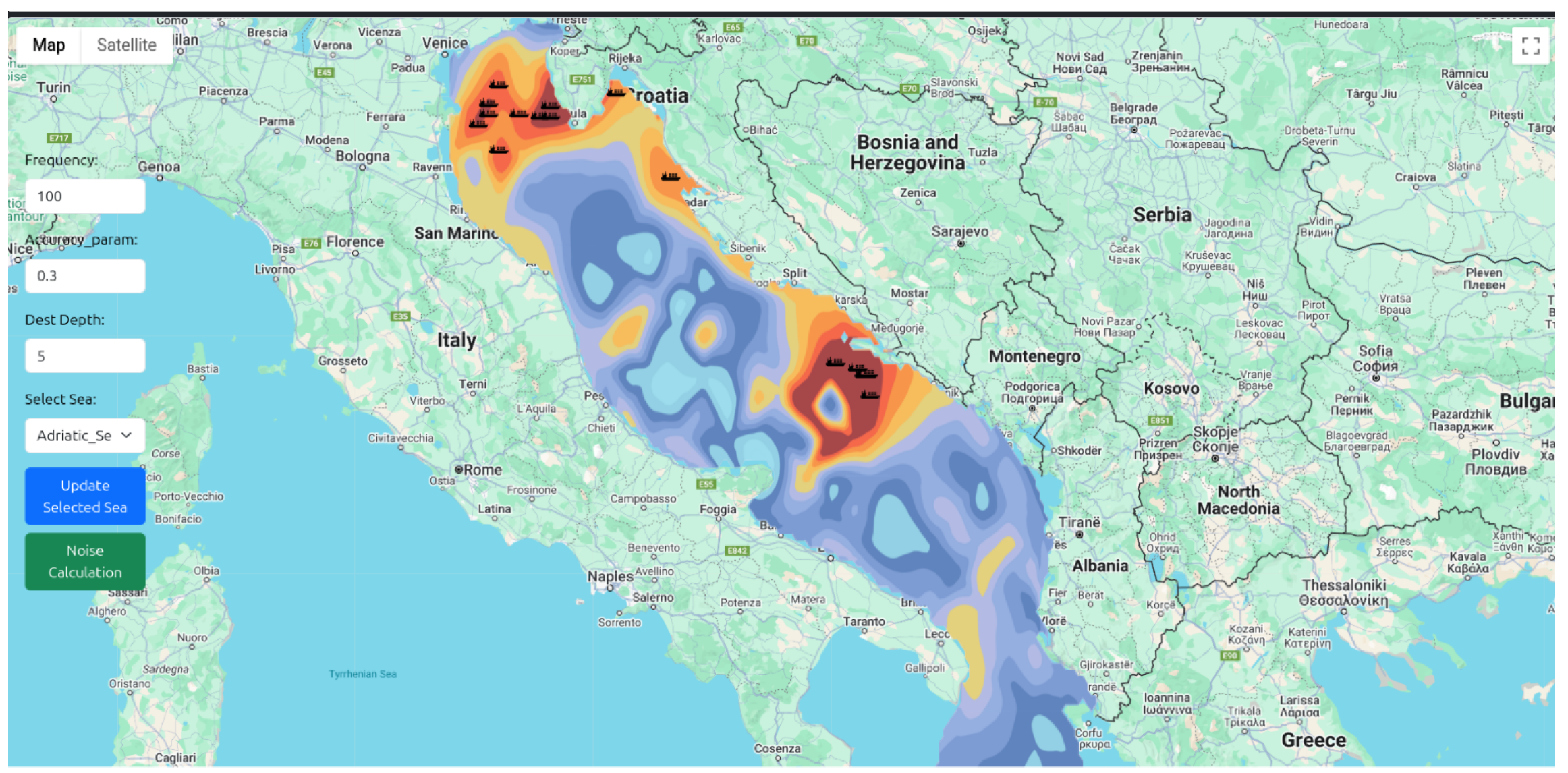
Consider now the Adriatic sea area. Figure 21 shows radiated ship noise at 10 pm on 8 May 2025. The main noise sources are located in the northern section of the basin, between the Venice area and the Istrian peninsula, as well as near the Split area in southern Croatia. The propagation of the noise generated by these ships is not very uniform due to the bathymetry of the Adriatic sea. Noise radiation tends to affect mainly local areas more than remote ones, with a few occurrences of insonification farther from the originating ships (e.g., off the Italian coast near Pescara (central Italy) and Lecce (southern Italy).

4.2. Airgun Noise Emission

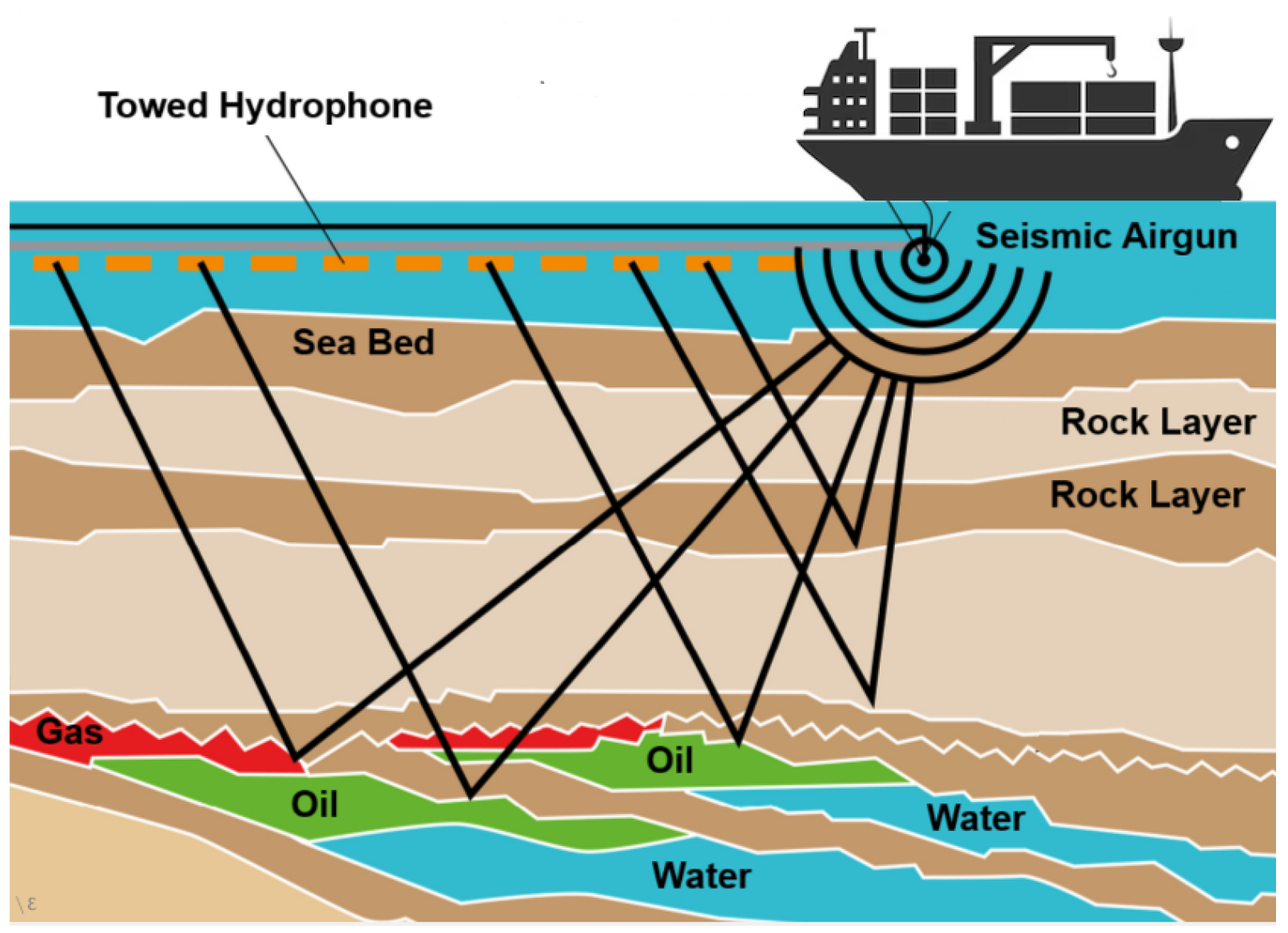
Seismic airguns are frequently utilized in geophysical prospections, and specifically in seismic seabed exploration, typically for mapping subsurface structures for oil, gas, and minerals. Airguns are typically arranged into arrays (e.g., of size 2 × 2) suspended on floaters and towed by a vessel. Each airgun generates repeatable pulses with source sound pressure levels up to 260 dB re 1 µPa (peak-to-peak) in the frequency band from 5 to 300 Hz [63]. Other uses of airguns include investigating tectonic features, fault lines, and sediment layers in geological studies, as well as studying subsurface water channels, volcanoes, or gas hydrates.
Figure 22 shows the general arrangement of an airgun seismic survey. Some studies report that airgun pulses from deep-water surveys were recorded at distances of more than 500 km, while pulses from shallow-water surveys were detected up to approximately 100 km [64].
Although seismic surveys are essential for seabed exploration, their high noise levels can negatively affect marine life. The work in [65] reports that the respiration rate of cephalopods may be affected by low-frequency seismic sound. It recorded respiratory suppression in Octopus ocellatus when they were exposed to low-frequency noise (50–150 Hz) at levels of about ≈120 dB re 1 μPa. The work in [66] shows bowhead whales change migration and move away at ≈120 dB re 1 μPa.
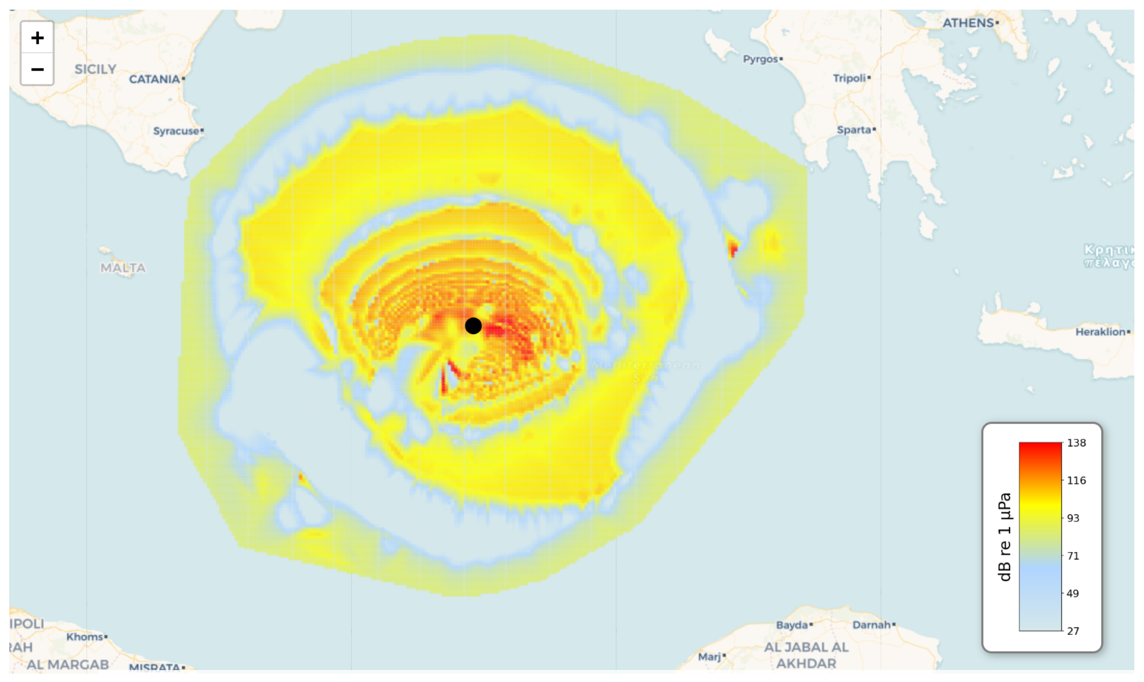
Using MNAT, it is possible to derive the noise intensity map at a frequency of 100 Hz that would originate from an airgun pulse fired between Sicily and the Peloponissos, in the Mediterranean sea. Figure 23 shows the noise map. Noise prediction is distributed around the firing point at coordinates ( 35.48 ° N , 18.33 ° E ) . The local sea depth at this point is 3860 m. With the aforementioned airgun blasting, a noise level of approximately 100 dB re 1 μPa is received at a distance of 400 km from the source.
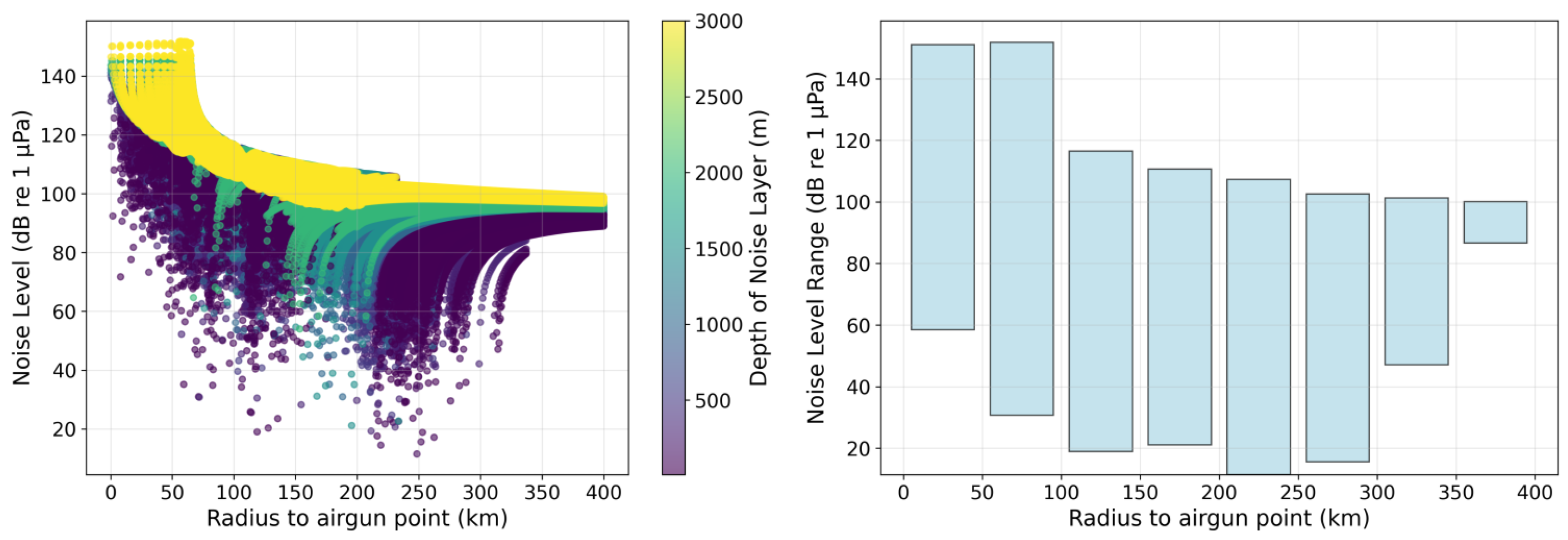
In an analysis, for the aforementioned airgun setting and location, the MNAT prediction model was applied across multiple depth layers (10, 25, 50, 100, 300, 1000, 1500, 2000, and 3000 m), in order to identify the areas of high risk for marine mammals. If we set ≈120 dB re 1 μPa as a threshold for potential impact on marine life, results indicate that within a range of 100 km from the airgun, the marine fauna is affected by the high-intensity noise due to the blast. This is also shown in Figure 24, where the left panel plots one dot for each correspondence of noise level (y-axis) received at a given range (x-axis). Each dot is colored according to the depth of the received location. The right panel considers distance intervals and conveys the range of the received noise level via a box plot. While the stronger noise blasts are heard at short ranges up to 100 km, we also observe that the noise level remains highest at deeper locations surrounding the blast area, regardless of the range.

5. Conclusions

This paper presented the MNAT, a framework designed to model, examine, and forecast underwater noise pollution. For shipping noise, MNAT combines AIS data with acoustic propagation models and real-time environmental inputs to provide a comprehensive framework for noise mapping, impact assessment, and mitigation strategy development. In addition, MNAT can manage noise from any set of point sources, including those that have a non-uniform radiation pattern.
MNAT addresses such challenges as large-scale data integration, outlier detection, complexity reduction via multiple modeling techniques, and user-friendly visualization in underwater acoustic propagation simulation. It aims to translate data into actionable recommendations for marine conservation, regulatory compliance, and sustainable maritime practices. It might be used in the identification of the effect of background noise on sonar and underwater communication systems, especially in regions near vessels or construction, where high levels of noise can interrupt signal detection and interpretation. In marine renewable energies, it can be used to simulate operation and construction noise to test their effect on acoustic marine ecosystems. It can also be applied by researchers in detailed underwater sound propagation studies using realistic environmental data and techniques of advanced modeling. As maritime trade expands and vessel traffic surges, this tool could also support marine traffic monitoring and safety, providing meaningful insights into noise risk and vessel monitoring in the congested sea routes.
Future work includes the modeling of additional types of noise sources, the implementation of wave patterns, and the incorporation of weather phenomena. Moreover, a limitation of this study is that the suggested methodologies have yet to be corroborated with in situ acoustic measurements. While deviations between modeled underwater radiated noise intensity and on-site measurements are inevitable, in situ data would greatly help confirm the validity of the models and point to deviations that suggest important noise sources. To address this, we are forming partnerships with oceanographic institutes working on airgun-based subsea prospection in order to collect observational datasets over the course of 2026. This will help us better validate our methods in future work.

Author Contributions

Conceptualization, M.R.T. and P.C.; Methodology, M.R.T. and P.C.; Software, M.R.T.; Data curation, M.R.T.; Writing—original draft, M.R.T. and P.C.; Writing—review & editing, P.C.; Visualization, M.R.T.; Supervision, P.C.; Project administration, P.C.; Funding acquisition, P.C. All authors have read and agreed to the published version of the manuscript.

Funding

This work was supported in part by the European Union—Next Generation EU, Mission 4 Component 2–CUP E63C22001030007 (project iNEST).

Data Availability Statement

The code presented in this study is available at https://git.manta.disi.unitn.it/mrtanhatalab/M-NAT (accessed on 21 October 2025).

Conflicts of Interest

The authors declare no conflicts of interest. The funders had no role in the design of the study; in the collection, analyses, or interpretation of data; in the writing of the manuscript; or in the decision to publish the results.

Abbreviations

AISAutomatic Identification System
APIApplication Programming Interface
ATAcoustic Toolbox
COGCourse Over Ground
GEBCOGeneral Bathymetric Chart of the Oceans
GISGeographic Information System
GPSGlobal Positioning System
GMMGaussian Mixture Model
GNNGraph Neural Network
GPRGaussian Process Regression
HSCHigh Speed Craft
IDWInverse Distance Weighting
ITUInternational Telecommunication Union
LATLatitude
LONLongitude
LSTMLong Short-Term Memory
MAEMean Absolute Error
MLMachine Learning
MLPMultilayer Perceptron
MNATMarine Noise Analysis Tool
MMSIMaritime Mobile Service Identity
NBNaïve Bayes
OASESOcean Acoustics and Seismic Exploration Synthesis
PDFProbability Density Function
PEParabolic Equation
RAMRange-Dependent Acoustic Model
RBFRadial Basis Function
RMSERoot Mean Squared Error
SLSource Level
SQLStructured Query Language
SOGSpeed Over Ground
SRStacking Regressor
SSPSound Speed Profile
SVMSupport Vector Machine
WOSSWorld Ocean Simulation System

References

  1. Markus, T.; Sánchez, P.P.S. Managing and Regulating Underwater Noise Pollution. In Handbook on Marine Environment Protection: Science, Impacts and Sustainable Management; Salomon, M., Markus, T., Eds.; Springer International Publishing: Cham, Switzerland, 2018; pp. 971–995. [Google Scholar] [CrossRef]
  2. Küsel, E.T.; Siderius, M. Comparison of Propagation Models for the Characterization of Sound Pressure Fields. IEEE J. Ocean. Eng. 2019, 44, 598–610. [Google Scholar] [CrossRef]
  3. Collins, M.D. A split-step Padé solution for the parabolic equation method. J. Acoust. Soc. Am. 1993, 93, 1736–1742. [Google Scholar] [CrossRef]
  4. Porter, M.B. The BELLHOP Manual and User’s Guide: Preliminary Draft; Technical Report; Beam/ray tracing model for ocean acoustics; Naval Research Laboratory: Washington, DC, USA, 1992. [Google Scholar]
  5. Zhang, L.; Meng, C. Modeling of Radiated Noise Passing Characteristic for Ship in Different Marine Environments. In Proceedings of the 2018 3rd International Conference on Modelling, Simulation and Applied Mathematics (MSAM 2018), Shanghai, China, 22–23 July 2018; Available online: https://api.semanticscholar.org/CorpusID:160002924 (accessed on 21 October 2025). [CrossRef]
  6. Neenan, S.T.V.; White, P.R.; Leighton, T.G.; Shaw, P.J. Modeling vessel noise emissions through the accumulation and propagation of Automatic Identification System data. In Proceedings of the Fourth International Conference on the Effects of Noise on Aquatic Life, Dublin, Ireland, 10–16 July 2016. [Google Scholar] [CrossRef]
  7. Racca, R.; Ainslie, M.A.; Bosschers, J.; Hermans, M.; Lloyd, T.; MacGillivray, A.O.; Pace, F.; Schuster, M.; Sertlek, Ö.; Wood, M.A. NAVISON Final Report: Calculation and analysis of shipping sound maps for all European seas from 2016 to 2050. J. Acoust. Soc. Am. 2024. [Google Scholar]
  8. Hartstra, I.; Salomons, E.M.; Colin, M.; Prior, M.K. Environment dependent transition frequencies for RAM and Bellhop. In Proceedings of the UACE 2019, Hersonissos, Greece, 30 June–5 July 2019; Available online: https://api.semanticscholar.org/CorpusID:199119962 (accessed on 21 October 2025).
  9. Larayedh, R.; Cornuelle, B.D.; Krokos, G.; Hoteit, I. Numerical investigation of shipping noise in the Red Sea. Sci. Rep. 2024, 14, 5851. [Google Scholar] [CrossRef]
  10. Durofchalk, N.C.; Doran, A.K.; Torres, J.R. Modeling sea surface noise in the presence of seamounts and ocean fronts using Nx2D and 3-D methods. J. Acoust. Soc. Am. 2023, 154, A355. [Google Scholar] [CrossRef]
  11. Laws, N. A Parabolic Equation Analysis of the Underwater Noise Radiated by Impact Pile Driving. Master’s Thesis, Portland State University, Portland, OR, USA, 2013. [Google Scholar] [CrossRef]
  12. Guelton, S.; Clorennec, D.; Pardo, E.; Brunet, P.; Folégot, T. Quonops©, la Prévision Opérationnelle en Acoustique Sous-Marine sur Grille de Calcul. 2013. Available online: https://api.semanticscholar.org/CorpusID:185456164 (accessed on 21 October 2025).
  13. Meng, C.; Xia, C.; Li, X.Y. Reconstruction and Evaluation of Ship Radiated Noise Signal in Ocean Channel. In Proceedings of the 2020 4th Annual International Conference on Data Science and Business Analytics (ICDSBA), Changsha, China, 5–6 September 2020; pp. 312–316. [Google Scholar] [CrossRef]
  14. Prokopovich, V.; Shafranyuk, A.V. Underwater radiated noise model of marine object. J. Phys. Conf. Ser. 2020, 1536, 012005. [Google Scholar] [CrossRef]
  15. Huang, I.L.; Lee, M.C.; Nieh, C.Y.; Huang, J.C. Ship Classification Based on AIS Data and Machine Learning Methods. Electronics 2023, 13, 98. [Google Scholar] [CrossRef]
  16. Wang, Y.; Wang, C.; Zhang, H. Ship Classification in High-Resolution SAR Images Using Deep Learning of Small Datasets. Sensors 2018, 18, 2929. [Google Scholar] [CrossRef]
  17. Luo, P.; Gao, J.; Wang, G.; Han, Y. Research on Ship Classification Method Based on AIS Data. In Proceedings of the Chinese Conference on Computer Supported Cooperative Work and Social Computing, Shenzhen, China, 7–9 November 2020. [Google Scholar] [CrossRef]
  18. Li, T.; Xu, H.; Zeng, W. Ship Classification Method for Massive AIS Trajectories Based on GNN. J. Phys. Conf. Ser. 2021, 2025, 012024. [Google Scholar] [CrossRef]
  19. Baeg, S.; Hammond, T.A. Ship Type Classification Based on The Ship Navigating Trajectory and Machine Learning. In Proceedings of the ACM IUI Workshops, Sydney, NSW, Australia, 27–31 March 2023; pp. 179–189. Available online: https://hdl.handle.net/1969.1/199814 (accessed on 21 October 2025).
  20. University of Washington. Ocean Noise Explorer (ONE). 2024. Available online: https://ocean-noise-explorer.readthedocs.io/en/latest/ (accessed on 21 October 2025).
  21. Cmst Web Team. Centre for Marine Science and Technology (CSMT)-Download AcTUP V2.2L Software. Online. 2009. Available online: https://api.semanticscholar.org/CorpusID:231077324 (accessed on 21 October 2025).
  22. Blue OASIS Software. 2024. Available online: https://blueoasis.pt/services/acoustics/ (accessed on 21 October 2025).
  23. ImageSoft. ImageSoft Tool. 2024. Available online: https://imagesoft.fi/ (accessed on 21 October 2025).
  24. Skylight. Skylight Tool. 2024. Available online: https://www.skylight.global/platform/ (accessed on 21 October 2025).
  25. Das, A. Indian Ocean Region (IOR) Mapping Platform. 2024. Available online: https://maritimeresearchcenter.com (accessed on 21 October 2025).
  26. Andrew, R.; Miksis-Olds, J.L.; Dugan, P.J.; Martin, S.B.; Klinck, H.; Mellinger, D.K.; Mann, D.A.; Ponirakis, D.; Boebel, O. Ocean Sound Analysis Software for Making Ambient Noise Trends Accessible (MANTA). Front. Mar. Sci. 2021, 8, 703650. [Google Scholar] [CrossRef]
  27. dBSea. dBSea, Underwater Noise Prediction and Visualisation Software. 2024. Available online: https://www.dbsea.co.uk/ (accessed on 21 October 2025).
  28. Park, M.H.; Yeo, S.; Choi, J.H.; Lee, W.J. Review of noise and vibration reduction technologies in marine machinery: Operational insights and engineering experience. Appl. Ocean. Res. 2024, 152, 104195. [Google Scholar] [CrossRef]
  29. Stream AIS. Websocket API Documentation. 2014. Available online: https://aisstream.io/ (accessed on 21 October 2025).
  30. Casari, P.; Tapparello, C.; Guerra, F.; Favaro, F.; Calabrese, I.; Toso, G.; Azad, S.; Masiero, R.; Zorzi, M. Open source suites for underwater networking: WOSS and DESERT underwater. IEEE Netw. 2014, 28, 38–46. [Google Scholar] [CrossRef]
  31. World Ocean Atlas (WOA). 2025. Available online: http://www.nodc.noaa.gov (accessed on 21 October 2025).
  32. General Bathymetric Chart of the Oceans. GEBCO. 2025. Available online: www.gebco.net (accessed on 21 October 2025).
  33. National Geophysical Data Center. Deck41, Seafloor Surficial Sediment Descriptions. 2025. Available online: https://www.ncei.noaa.gov/access/metadata/landing-page/bin/iso?id=gov.noaa.ngdc.mgg.geology:G02094 (accessed on 21 October 2025).
  34. International Telecommunication Union. Technical Characteristics for an Automatic Identification System Using Time Division Multiple Access in the VHF Maritime Mobile Frequency Band, 2014. Recommendation ITU-R M.1371-5. Available online: https://www.itu.int/rec/R-REC-M.1371-5-201402-I (accessed on 21 October 2025).
  35. Gandhi, I.; Pandey, M. Hybrid Ensemble of classifiers using voting. In Proceedings of the 2015 International Conference on Green Computing and Internet of Things (ICGCIoT), Greater Noida, India, 8–10 October 2015; pp. 399–404. [Google Scholar] [CrossRef]
  36. Breiman, L. Random Forests. Machine Learning. Mach. Learn. 2001, 45, 5–32. [Google Scholar] [CrossRef]
  37. Chen, T.; Guestrin, C. XGBoost: A Scalable Tree Boosting System. arXiv 2016. [Google Scholar] [CrossRef]
  38. Hearst, M.; Dumais, S.; Osuna, E.; Platt, J.; Scholkopf, B. Support vector machines. IEEE Intell. Syst. Their Appl. 1998, 13, 18–28. [Google Scholar] [CrossRef]
  39. Rokach, L.; Maimon, O. Decision Trees. In Data Mining and Knowledge Discovery Handbook; Maimon, O., Rokach, L., Eds.; Springer: Boston, MA, USA, 2005; pp. 165–192. [Google Scholar] [CrossRef]
  40. Mucherino, A.; Papajorgji, P.J.; Pardalos, P.M. k-Nearest Neighbor Classification. In Data Mining in Agriculture; Springer: New York, NY, USA, 2009; pp. 83–106. [Google Scholar] [CrossRef]
  41. Anand, M.V.; KiranBala, B.; Srividhya, S.R.; Kavitha, C.; Younus, M.; Rahman, M.H.; Kumar Reddy, M.P. Gaussian Naïve Bayes Algorithm: A Reliable Technique Involved in the Assortment of the Segregation in Cancer. Mob. Inf. Syst. 2022, 2022, 2436946. [Google Scholar] [CrossRef]
  42. Nassara, E.I.G.; Grall-Maës, E.; Kharouf, M. Linear Discriminant Analysis for Large-Scale Data: Application on Text and Image Data. In Proceedings of the 2016 15th IEEE International Conference on Machine Learning and Applications (ICMLA), Anaheim, CA, USA, 18–20 December 2016; pp. 961–964. [Google Scholar] [CrossRef]
  43. Biggs, F.; Zantedeschi, V.; Guedj, B. On Margins and Generalisation for Voting Classifierse. 2022. Available online: https://arxiv.org/pdf/2206.04607 (accessed on 21 October 2025).
  44. Parsons, M.J.G.; Erbe, C.; Meekan, M.G.; Parsons, S.K. A Review and Meta-Analysis of Underwater Noise Radiated by Small (<25 m Length) Vessels. J. Mar. Sci. Eng. 2021, 9, 827. [Google Scholar] [CrossRef]
  45. Lloyd, T.; Daniel, J.; Bosschers, J.; Schuster, M. ‘PIANO’: A physics-based semi-empirical source level model for fleet-scale ship URN prediction. In Proceedings of the Eighth International Symposium on Marine Propulsors Smp’24, Berlin, Germany, 17–20 March 2024. [Google Scholar] [CrossRef]
  46. Veirs, S.; Veirs, V.; Wood, J.D. Ship noise extends to frequencies used for echolocation by endangered killer whales. PeerJ 2016, 4, e1657. [Google Scholar] [CrossRef] [PubMed]
  47. Last, P.; Bahlke, C.; Hering-Bertram, M.; Linsen, L. Comprehensive Analysis of Automatic Identification System (AIS) Data in Regard to Vessel Movement Prediction. J. Navig. 2014, 67, 791–809. [Google Scholar] [CrossRef]
  48. Nguyen, D.; Fablet, R. A Transformer Network with Sparse Augmented Data Representation and Cross Entropy Loss for AIS-Based Vessel Trajectory Prediction. IEEE Access 2021, 12, 21596–21609. [Google Scholar] [CrossRef]
  49. Ke, G.; Meng, Q.; Finley, T.; Wang, T.; Chen, W.; Ma, W.; Ye, Q.; Liu, T.Y. LightGBM: A Highly Efficient Gradient Boosting Decision Tree. In Advances in Neural Information Processing Systems; Guyon, I., Luxburg, U.V., Bengio, S., Wallach, H., Fergus, R., Vishwanathan, S., Garnett, R., Eds.; Curran Associates, Inc.: Red Hook, NY, USA, 2017; Volume 30, Available online: https://proceedings.neurips.cc/paper_files/paper/2017/file/6449f44a102fde848669bdd9eb6b76fa-Paper.pdf (accessed on 21 October 2025).
  50. Prokhorenkova, L.; Gusev, G.; Vorobev, A.; Dorogush, A.V.; Gulin, A. CatBoost: Unbiased boosting with categorical features. In Advances in Neural Information Processing Systems; Bengio, S., Wallach, H., Larochelle, H., Grauman, K., Cesa-Bianchi, N., Garnett, R., Eds.; Curran Associates, Inc.: Red Hook, NY, USA, 2018; Volume 31, Available online: https://proceedings.neurips.cc/paper_files/paper/2018/file/14491b756b3a51daac41c24863285549-Paper.pdf (accessed on 21 October 2025).
  51. McDonald, G.C. Ridge regression. WIREs Comput. Stat. 2009, 1, 93–100. [Google Scholar] [CrossRef]
  52. Reynolds, D. Gaussian Mixture Models. In Encyclopedia of Biometrics; Li, S.Z., Jain, A., Eds.; Springer: Boston, MA, USA, 2009; pp. 659–663. [Google Scholar] [CrossRef]
  53. Cometti, D.S.; Mazuelas, S.; Sacco, G.; Melazzi, N.B.; Bartoletti, S. Location-Aided Iterative Beam Search via Learning-based Generative Models. In Proceedings of the 2025 IEEE International Conference on Communications Workshops (ICC Workshops), Montreal, QC, Canada, 8–12 June 2025; pp. 1906–1911. [Google Scholar] [CrossRef]
  54. Huang, H.; Cui, C.; Cheng, L.; Liu, Q.; Wang, J. Grid interpolation algorithm based on nearest neighbor fast search. Earth Sci. Inf. 2012, 5, 181–187. [Google Scholar] [CrossRef]
  55. Amidror, I. Scattered data interpolation methods for electronic imaging systems: A survey. J. Electron. Imaging 2002, 11, 157–176. [Google Scholar] [CrossRef]
  56. Worsey, A.; Farin, G. Ann-dimensional Clough-Tocher interpolant. Constr. Approx. 1987, 3, 99–110. [Google Scholar] [CrossRef]
  57. Chen, C.; Li, Y.; Zhao, N.; Guo, B.; Mou, N. Least Squares Compactly Supported Radial Basis Function for Digital Terrain Model Interpolation from Airborne Lidar Point Clouds. Remote Sens. 2018, 10, 587. [Google Scholar] [CrossRef]
  58. Benmoshe, N. A Simple Solution for the Inverse Distance Weighting Interpolation (IDW) Clustering Problem. Sci 2025, 7, 30. [Google Scholar] [CrossRef]
  59. Raid, I.; Kusnezowa, T.; Seewig, J. Application of ordinary kriging for interpolation of micro-structured technical surfaces. Meas. Sci. Technol. 2013, 24, 095201. [Google Scholar] [CrossRef]
  60. Chang, C.; Zeng, T. A hybrid data-driven-physics-constrained Gaussian process regression framework with deep kernel for uncertainty quantification. J. Comput. Phys. 2023, 486, 112129. [Google Scholar] [CrossRef]
  61. Rasmussen, C.E.; Williams, C.K.I. White noise kernel. In Gaussian Processes for Machine Learning; Springer International Publishing: Berlin/Heidelberg, Germany, 2006; Available online: https://gaussianprocess.org/gpml/ (accessed on 21 October 2025).
  62. Lu, G.Y.; Wong, D.W. An adaptive inverse-distance weighting spatial interpolation technique. Comput. Geosci. 2008, 34, 1044–1055. [Google Scholar] [CrossRef]
  63. Turner, S.; Zykov, M.; MacGillivray, A. Preliminary Acoustic Level Measurements of Airgun Sources from Conoco Phillips’ 2006 Seismic Survey in Alaskan Chukchi Sea; JASCO Research Ltd.: Victoria, BC, Canada, 2006. [Google Scholar]
  64. Keen, K.A.; Thayre, B.J.; Hildebrand, J.A.; Wiggins, S.M. Seismic airgun sound propagation in Arctic Ocean waveguides. Deep. Sea Res. Part I Oceanogr. Res. Pap. 2018, 141, 24–32. Available online: https://api.semanticscholar.org/CorpusID:53056420 (accessed on 21 October 2025). [CrossRef]
  65. Kaifu, K.; Segawa, S.; Tsuchiya, K. Behavioral Responses to Underwater Sound in the Small Benthic Octopus Octopus ocellatus. J. Mar. Acoust. Soc. Jpn. 2007, 34, 266–273. [Google Scholar] [CrossRef]
  66. Blackwell, S.B.; Nations, C.S.; McDonald, T.L.; Thode, A.M.; Mathias, D.; Kim, K.H.; Greene, C.R., Jr.; Macrander, A.M. Effects of Airgun Sounds on Bowhead Whale Calling Rates: Evidence for Two Behavioral Thresholds. PLoS ONE 2015, 10, e0125720. [Google Scholar] [CrossRef] [PubMed]
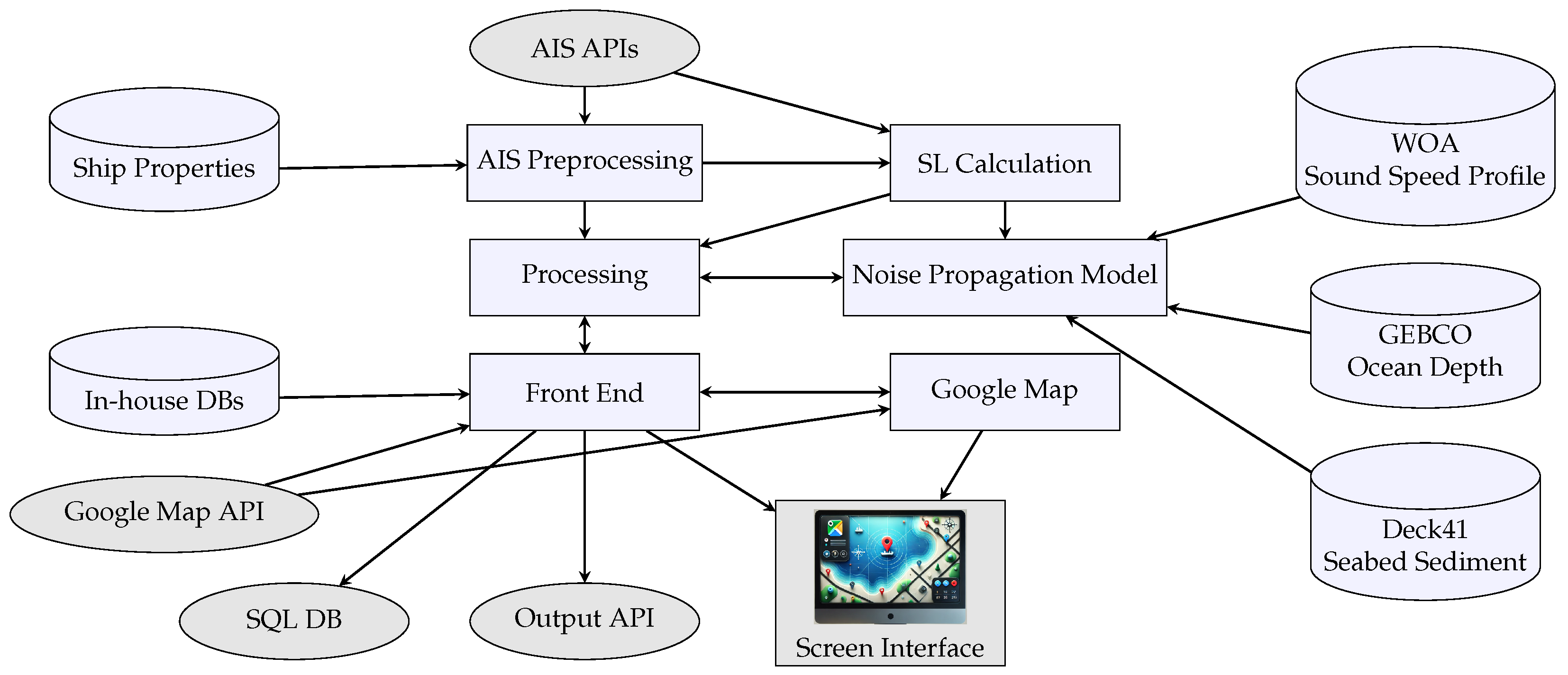
Figure 1. Architecture of MNAT.
Jmse 13 02045 g001
Figure 2. The tool interface can show the vessels’ trajectory. This figure depicts 90 min of ship navigation in the north of the Adriatic sea between Italy, Slovenia, and Croatia. The red line shows the ships’ trajectory, and the arrow shows the direction of the path.
Jmse 13 02045 g002
Figure 3. Ship type count per category for 35,471 ships collected over a 40-day window between 2 March 2025, and 11 April 2025, across global seas. Ship types are classified into 4 classes: normal in blue, not assigned in red, reserved for future in pink, and ship type numbers above 100 in green. Problematic data (not assigned ship types, reserved type, and ship type above 100) amount to 6% of the dataset.
Jmse 13 02045 g003
Figure 4. Architecture of ship-type prediction.
Jmse 13 02045 g004
Figure 5. Ship geometry parameters used in ship-type prediction. The gray circle represent the location of the AIS antenna.
Jmse 13 02045 g005
Figure 6. Distributed AIS draught values for 35,471 ships, collected globally. Outliers are shown as dots for each ship type.
Jmse 13 02045 g006
Figure 7. AIS SOG data for 18,240,266 ships collected globally. The figure shows that reported SOG values range from 0 to 100 knots. The box plot summarizes the distribution of SOG values for each ship type. Outliers are represented as individual dots.
Jmse 13 02045 g007
Figure 8. Median source spectrum levels for different vessel classes.
Jmse 13 02045 g008
Figure 9. Quantiles of noise source levels across different vessel classes as a function of frequency.
Jmse 13 02045 g009
Figure 10. AIS-based vessel trajectory predictions: The blue lines represent all types of vessel trajectories across European waters over a 40-day period from 2 March 2025 to 11 April 2025. The highlighted red points show AIS reports from the FURE SPEAR tanker (MMSI: 231894000). The orange points represent actual AIS positions that are used for comparison against the predicted trajectory, as shown in yellow.
Jmse 13 02045 g010
Figure 11. AIS recorded locations of vessels in the Adriatic sea whose noise maps are used as training data for the GMM. Light blue dots represent location readings. The center of each cluster obtained through the GMM is depicted as a red cross. Green dots represent vessels extracted from AIS APIs in a later run of MNAT and assigned to the most likely cluster for training the Stacking Regressor.
Jmse 13 02045 g011
Figure 12. Acoustic model estimation (right) and stacking regressor prediction (left) for a single ship’s radiated noise in the Adriatic sea.
Jmse 13 02045 g012
Figure 13. Obstacles and islands (red areas) detection in the Sulu sea.
Jmse 13 02045 g013
Figure 14. Regular and optimized coastline points selection. (a) Irregular distribution method. (b) Optimized uniform selection.
Jmse 13 02045 g014
Figure 15. (Left) Regular rectangular grid with 1224 points covering the Adriatic sea for noise intensity evaluation. (Right) Circular grid approach with 70 sectors. Each fan is directed from the noise source to one of the coastline points determined via the procedure in Section 3.3.3.
Jmse 13 02045 g015
Figure 16. Left figure shows the Bellhop model estimation for each point in the regular grid approach that is considered as ground truth. The right plot is the Bellhop model estimation for a circular grid system that is calculated for each selected coastline point relative to the noise source.
Jmse 13 02045 g016
Figure 17. Comparison of different interpolation methods for transmission loss in the Adriatic sea. The noise source is at coordinates ( 43.24 ° N , 14.59 ° E ) .
Jmse 13 02045 g017
Figure 18. Deviation of sound intensity maps from the ground truth. The interpolated values tend to be lower than the ground truth near the coastline after the deep water, whereas they are higher than the ground truth in the vicinity of the noise source and where there is a sudden change in slope.
Jmse 13 02045 g018
Figure 19. Google Earth screenshot showing the bathymetry of the Bay of Biscay.
Jmse 13 02045 g019
Figure 20. MNAT-computed noise map for the Bay of Biscay. We observe a significant match between radiated noise levels and the bathymetry of the area. Dark red hues represent high noise, whereas yellow, dark blue, and light blue hues convey progressively lower noise levels.
Jmse 13 02045 g020
Figure 21. MNAT-computed noise map for the Adriatic sea. The number of ships and sea properties, like the type of seafloor or bathymetry, affect noise propagation. Dark red hues represent high noise, whereas yellow, dark blue, and light blue hues convey progressively lower noise levels.
Jmse 13 02045 g021
Figure 22. Schematic view of marine seismic surveying using airguns and hydrophone arrays. Different sea bottom layers are illustrated in various colors: blue denotes water, brown hues convey different types of rock, red represents gas, and green indicates oil beneath the seabed.
Jmse 13 02045 g022
Figure 23. Propagated airgun noise in the Mediterranean sea for an underwater airgun explosion. The oscillating intensity of propagated noise reflects the lobes in the radiation pattern of the airgun. Like in previous results, we observe that bathymetry affects noise propagation significantly.
Jmse 13 02045 g023
Figure 24. Propagated noise at different depths and at different ranges in the Mediterranean sea after an airgun firing at coordinates ( 35.48 ° N , 18.33 ° E ) . The scatterplot in the left panel illustrates the noise levels as a function of range (x-axis) and depth (dot color). The box plot in the right panel depicts noise ranges at different distance intervals.
Jmse 13 02045 g024
Table 1. Comparison of MNAT against other underwater radiated noise modeling tools.
FeaturedBSeaMANTAAcTUPMNAT (Proposed)
ScalabilityScenario-limited, solver-dependent.Processes large soundscape archives, but in only batch mode.Allows batch runs of multiple acoustic toolbox methods; research-grade, MATLAB-dependent.Designed for basin- and sea-level simulations with real-time multi-vessel handling; use goes beyond research contexts.
SpeedAdvanced solvers (e.g., PE) can be slow.Batch postprocessing can be slow.Moderate; solver-dependent, not optimized for real-time.Standard models may be slow, but machine learning used in parallel accelerates their performance.
UsabilityRequires acoustic expertise and manual tuning.GUI with calibration support, but requires technical knowledge.Menu-driven MATLAB interface; automated acoustic tool integration.Web-based geographical GUI; automated AIS preprocessing and ML-aided vessel classification.
Innovation gapValidated propagation models for scenario accuracy.Standardized noise datasets for comparability.Unifies acoustic tool codes in one interface with batch capability.Integrates preprocessed real-time AIS data, estimates source noise levels close to reality, leverages machine learning to accelerate processing, and offers a scalable web-based simulation with interactive visualization.
Table 2. Schemas of the PositionData and ShipStaticData tables.
AttributeTypeDescription
PositionData table
UserIDIntegerUnique vessel identifier
CogFloatCourse over ground in degrees
LatitudeFloatVessel’s latitude coordinate
LongitudeFloatVessel’s longitude coordinate
MessageIDIntegerAIS message type identifier
NavigationalStatusIntegerVessel’s operational status (e.g., underway, anchored, moored)
RateOfTurnFloatRate of turn in degrees per minute
SogFloatSpeed over ground in knots
TimestampIntegerUnix timestamp of the position report
TrueHeadingIntegerVessel’s true heading in degrees
UpdatedTimeDateTimeDatabase update timestamp
ShipStaticData table
UserIDIntegerUnique vessel identifier (primary key)
DimensionAIntegerDistance from reference point to bow
DimensionBIntegerDistance from reference point to stern
DimensionCIntegerDistance from reference point to port side
DimensionDIntegerDistance from reference point to starboard
ImoNumberIntegerInternational Maritime Organization number
MaximumStaticDraughtFloatMaximum static draught in meters
MessageIDIntegerAIS message type identifier
TypeIntegerShip-type classification
UpdatedTimeDateTimeDatabase update timestamp
Table 3. Detailed evaluation metrics of ML models for vessel type Classification.
PrecisionRecallF1-Score
Model Cargo Fishing Tanker Cargo Fishing Tanker Cargo Fishing Tanker Accuracy
Voting Classifier0.900.940.890.920.990.820.910.970.860.91
Random Forest0.900.950.900.930.990.830.910.970.870.91
XGBoost0.910.950.890.920.990.840.910.970.860.91
SVM0.840.930.700.780.990.740.810.960.720.81
Decision Tree0.860.940.820.880.940.790.870.940.800.87
KNN0.810.940.730.830.990.680.820.960.700.81
Gaussian NB0.660.910.580.840.950.300.740.930.400.70
Logistic Regression0.760.910.590.710.990.620.740.950.610.74
LDA0.720.940.800.910.950.430.800.940.560.78
Table 4. Performance of noise prediction models, ordered from best to worst according to MAE, RMSE, and R 2 .
ModelMAE (dB)RMSE (dB) R 2 (Ratio)
Stacking Regressor2.63.20.98
XGBoost2.73.40.98
CatBoost2.93.60.98
Random Forest3.44.30.97
LightGBM3.44.30.97
Extra Trees3.44.30.97
Gradient Boosting3.64.50.97
Voting Regressor4.05.00.96
KNN6.48.00.92
Table 5. GMM-based vessel ranking.
RankVesselPositionClosest ClusterScore
1v8(45.17, 12.78)C096.3
2v5(44.86, 12.97)C094.9
3v12(44.87, 13.02)C094.9
4v2(40.75, 18.68)C393.8
5v1(40.54, 18.89)C392.1
6v10(45.45, 13.35)C091.3
7v4(44.74, 13.17)C091.2
8v13(44.68, 12.88)C091.0
9v14(44.67, 13.04)C090.9
10v9(44.62, 12.72)C088.8
11v3(43.24, 14.59)C285.5
12v11(44.31, 12.64)C082.6
13v7(43.81, 15.00)C174.3
14v6(42.08, 16.00)C263.5
Table 6. Sequence of vessels selected to be added to the training dataset for machine learning interpolation algorithms.
Pick sequence1234567891011121314
Global rank1411131210981457632
Vesselv8v2v3v7v11v9v14v13v6v1v4v10v12v5
ClusterC0C3C2C1C0C0C0C0C2C3C0C0C0C0
Table 7. Interpolation methods and their hyperparameters.
MethodParameterValue
RBFFunctioncubic
Epsilon9.7088
IDWPower4.9987
GPR-PhysicsWhite Kernel noise level0.01
RBF Kernel length scale0.1
Alpha 1.60 × 10 6
Restarts optimizer15
KrigingVariogram modelExponential
Nugget0.0015
Sill4.0368
Range8.6882
Griddata (Nearest)Fill valueNaN
Griddata (Linear)Fill valueNaN
Clough-TocherTriangulation methodConvex hull
Interpolation orderLinear
Boundary handlingExtrapolate
Fill valueNaN
Ensemble MultiMethods PhysicsIDW Weight60%
Other Methods Weight40%
Distance MetricEuclidean
Matching StrategyNearest Neighbor
Spatial ResolutionGrid-based
Disclaimer/Publisher’s Note: The statements, opinions and data contained in all publications are solely those of the individual author(s) and contributor(s) and not of MDPI and/or the editor(s). MDPI and/or the editor(s) disclaim responsibility for any injury to people or property resulting from any ideas, methods, instructions or products referred to in the content.