Underwater Target Search Path Planning Based on Sound Speed Profile Clustering and Improved Ant Colony Optimization

Abstract

To address the problems of low efficiency and poor real-time performance in underwater acoustic modeling, as well as the requirement of maximizing search coverage for underwater target search path planning, this paper proposed an efficient path planning method based on Sound Speed Profile (SSP) clustering. Firstly, the SSPs were dimensionally reduced via Empirical Orthogonal Function (EOF) decomposition, and the sea area was divided into 10 acoustic sub-areas using K-means clustering after fusing geographic coordinates and terrain information, thereby constructing a block-wise sound field model. Secondly, with the active sonar equation as the core, sonar parameters such as the noise level and target strength were solved, respectively, to generate a spatial distribution matrix of search distances. Finally, an Improved Ant Colony Optimization (IACO) algorithm was modified by dynamically setting the pheromone evaporation rate and improving the heuristic information for search path optimization. Numerical experiments showed that clustering significantly improves the efficiency of sound field modeling, reducing the time consumption of the transmission loss calculation from 24.74 h to 10.84 min. The IACO increased the average search coverage from 47.96% to 86.01%, with an improvement of 79.34%. The performance of IACO is superior to those of the compared algorithms, providing support for efficient underwater target search.

1. Introduction

With the growth of marine resource exploitation, underwater rescue and national defense demands, underwater target search technology has received extensive attention and development [1]. Searching for underwater targets such as underwater vehicles, personnel overboard, or materials in unknown sea areas is a highly challenging task. To efficiently accomplish the search mission, it is necessary to plan the search path of surface ships to ensure the maximization of their search coverage.

When surface ships perform path planning for searching underwater targets, the influence of the underwater acoustic environment must be fully considered. Sound waves are so far the only known form of energy suitable for long-distance propagation in seawater [2]; thus, the use of sonar systems to detect and analyze reflected or radiated sound waves from underwater targets constitutes the primary method for underwater target search. However, due to the particularity of the underwater acoustic environment, existing search methods still face numerous challenges [3]. The classical model of active sonar indicates that the attenuation of acoustic wave propagation affects the detection range of sonar [2]. Meanwhile, seabed sediments also influence the reflection coefficient of acoustic waves, causing attenuation of the echo intensity of active sonar; thus, a terrain compensation algorithm needs to be introduced in path planning [4]. The seabed is uneven, and seabed terrain roughness is one of the important factors affecting acoustic wave reflection, which should be considered in refined path planning [5]. Acoustic waves exhibit special propagation characteristics in complex underwater acoustic environments such as thermoclines and haloclines—for instance, sound channels can enable long-distance propagation of acoustic waves, and they can be utilized to extend the sonar detection range [6]. Various geological features and oceanographic processes may lead to horizontal reflection, refraction, and diffraction of underwater sound, thereby affecting the distribution of the underwater sound field and resulting in different sonar detection ranges in different sea areas [7]. Yu et al. [8], Ren & Zhang [9], and Ai [10], among others, incorporated the influences of reverberation mutations, acoustic detection probability, energy consumption and ocean currents, environmental noise levels, and sonar signal-to-noise ratio into path planning. Liao et al. [11] and Wang et al. [12] focused on integrating surface wind fields, seabed terrain, and transmission loss into path planning models, investigating path planning methods to maximize search coverage area. A growing number of scholars have recognized that the underwater acoustic environment exerts a significant impact on the path planning of surface ships. However, the complexity of the marine acoustic environment and boundary conditions limits the solution speed of refined underwater acoustic modeling. Classic studies have indicated that the traditional finite element-boundary element coupling method is significantly time-consuming for acoustic calculations of large-scale complex underwater structures, requiring 48 h to complete the calculation for a single scenario [13]. When simulating the propagation of deep-sea pulse sound sources, calculations for a 10 km propagation distance based on the second-order finite element method take 18 h [14]. In addition, when solving the eigenvalue problem using the normal mode model, if the number of SSP layers exceeds 100, a single calculation may take several hours, making it difficult to meet real-time requirements [15]. Therefore, there is an urgent need to find an efficient underwater acoustic modeling method to support the path planning of surface ships.

A practical approach is to perform clustering on the SSPs of the study sea area. The sound speed in seawater is affected by temperature, salinity, and pressure [16], and sound propagation is influenced by SSPs and seabed terrain. According to the first law of geography [17], temperature, salinity, pressure, and seabed terrain in adjacent sea areas exhibit strong spatial correlation; thus, SSPs and sound propagation also have spatial correlation. Based on the above spatial correlation, clustering SSPs and dividing the study sea area into sub-regions according to the types of SSPs for block-wise acoustic modeling can effectively address the problem of significant computational time caused by processing each point sequentially.

Against the above background, this study introduces SSP clustering and improves the Ant Colony Optimization (ACO) algorithm to propose an efficient path planning method for underwater target search. The main contributions of this paper are summarized as follows:

• Path planning is conducted with consideration of the influences of the underwater acoustic environment. Compared with traditional geometric path planning, this method fully accounts for the impacts of acoustic and topographic factors on the sonar detection range, and exhibits a higher level of refinement;
• Introduction of SSP clustering. Based on the spatial correlation of SSPs, the SSPs in adjacent sea areas with similar characteristics are clustered. This significantly reduces the high time consumption caused by the large spatial scale of the mission area;
• Improvement of the ACO algorithm. Aiming at the specific problem of path planning, the pheromone evaporation rate is dynamically set and the heuristic information is improved, resulting in its performance being superior to that of other benchmark algorithms.

The remaining sections of this paper are arranged as follows: Section 2 describes the research status of SSP clustering and path planning. Section 3 introduces the data sources, the method of SSP clustering, the method of estimating sonar search distance, and the design of the IACO algorithm. Section 4 presents the results of SSP clustering, sound field modeling, and path optimization, and analyzes the optimization effects brought by the introduction of SSP clustering and the IACO algorithm. Section 5 summarizes the entire work.

2. Related Work

Currently, most studies on SSP clustering focus on fields such as data reconstruction or marine acoustic effects, but there are few studies on path planning methods based on SSP clustering. In the field of data reconstruction, SSP clustering methods have been applied to reconstruct shallow-sea SSPs in the South China Sea [18], improve the reconstruction accuracy of EOF [19], verify the differences in sound channel axis depth among SSP types in the North Atlantic [20], and predict SSPs [21], among other aspects. In the field of marine acoustic effects, SSP clustering methods have been used to construct ocean front models [22], verify that the under-ice reverberation intensity has a strong correlation with ice layer thickness and acoustic wave frequency [23], and identify the depth of sound sources in complex under-ice acoustic environments in the Arctic [24], etc. However, in the field of underwater target search path planning, relatively few scholars have applied SSP clustering to relevant research.

A large number of scholars have conducted research in the field of path planning, including robot path planning and Autonomous Underwater Vehicle (AUV) path planning. Zhang et al. [25] proposed an underwater glider target search path planning method based on an improved particle swarm optimization algorithm. Liu et al. [26] applied an improved dual-population ant colony algorithm to solve the shortest path planning problem of underwater robots. Orozco-Rosas et al. [27,28] proposed the membrane evolutionary artificial potential field method and the QAPF learning algorithm in 2019 and 2022, respectively, to address the path planning problem of mobile robots. Wang et al. [29] proposed a knowledge hierarchy-based dynamic multi-objective optimization method for the path planning problem of AUVs in underwater cooperative search missions. Tang et al. [30] applied deep reinforcement learning to realize AUV path planning. However, in the context of this study, surface ships need to plan an optimal path to maximize search coverage for the purpose of maximizing the probability of detecting underwater targets, which differs from previous path planning focused on obstacle avoidance or navigation.

3. Data and Methods

The technical route of the underwater target search path planning method proposed in this paper is summarized into the following three points: First, cluster the SSPs in the study sea area to construct a block-wise underwater acoustic environment model. Second, use the marine sound propagation model to calculate the transmission loss of each block, and then combine other sonar parameters such as noise level, source level, and target strength to solve the spatial distribution matrix of the search distance of the active sonar in the entire sea area. Third, plan the search path of the surface ship and introduce the IACO algorithm for path optimization to maximize the search coverage. This section will clarify the sources of raw data and elaborate on the SSP clustering method, the sonar search distance estimation method, and the design of the IACO algorithm.

3.1. Data Sources

Marine acoustic models require data on sound speed, seabed topography, and sea surface wind speed as inputs. In this study, the data on temperature, salinity, and wind speed at 10 m above the sea surface were obtained from the Copernicus Marine Environment Monitoring Service (CMEMS) dataset, which represents the average of observational data on July 22, 2025. The temperature and salinity data, with a horizontal spatial resolution of 1/12˚ and 50 vertical layers (covering a water depth range of 0~5727.917 m), were used to calculate SSPs. The wind speed data at 10 m above the sea surface, with a horizontal spatial resolution of 1/8°, were utilized for computing noise levels. Bathymetric data were derived from ETOPO 2022, with a horizontal spatial resolution of 60″. As shown in Figure 1, the study area spans 22° N–25° N, 130° E–133° E, with an average water depth of 4680 m, belonging to the deep-sea region. Among them, the date and study sea area are randomly selected, while the proposed method is applicable to any date and any deep-sea area.

3.2. SSP Clustering

After acquiring the temperature, salinity, and pressure data of the mission sea area, the empirical formula for seawater sound speed is used to calculate SSPs. EOF decomposition is employed to achieve dimensionality reduction in the SSP data, which is then fused with geographic location and seabed terrain information. Finally, K-means clustering is adopted to classify the mission sea area according to the acoustic environment.

3.2.1. Calculation of SSP

In this study, the Chen-Millero-Li (1994) formula [31] is employed to calculate the sound speed in seawater. This formula, based on extensive experimental data, is widely applied in marine acoustics, underwater acoustic engineering, and marine scientific research. Its complete form is expressed as:

$$C(T,S,P)=C_W(T,P)+A(T,P)S+B(T,P)S^{3/2}+D(T,P)S^2+C_C(T,P),$$

(1)

$$\begin{array}{l}{C}_W(T,P)=(C_{00}+C_{01}T+C_{02}{T}^2+C_{03}{T}^3+C_{04}{T}^4+C_{05}{T}^5)+(C_{10}+C_{11}T+C_{12}{T}^2+C_{13}{T}^3+C_{14}{T}^4)P+\\ \hspace{1em}\hspace{1em}\hspace{1em}\hspace{1em} (C_{20}+C_{21}T+C_{22}{T}^2+C_{23}{T}^3+C_{24}{T}^4)P^2+(C_{30}+C_{31}T+C_{32}{T}^2)P^3\end{array},$$

(2)

$$\begin{array}{l}A(T,P)=(A_{00}+A_{01}T+A_{02}{T}^2+A_{03}{T}^3+A_{04}{T}^4)+(A_{10}+A_{11}T+A_{12}{T}^2+A_{13}{T}^3+A_{14}{T}^4)P+\\ \hspace{1em}\hspace{1em}\hspace{1em}\hspace{1em}(A_{20}+A_{21}T+A_{22}{T}^2+A_{23}{T}^3)P^2+(A_{30}+A_{31}T+A_{32}{T}^2)P^3\end{array},$$

(3)

$$B(T,P)=B_{00}+B_{01}T+(B_{10}+B_{11}T)P,$$

(4)

$$D(T,P)=D_{00}+D_{10}P,$$

(5)

$$C_C(T,P)=(R_{10}+R_{11}T+R_{12}{T}^2)P+(R_{20}+R_{21}T+R_{22}{T}^2)P^2+R_{31}{P}^3,$$

(6)

where C(T, S, P) denotes the sound speed in seawater, C_W(T, P) represents the sound speed in pure water, and C_C(T, P) is the correction term. T stands for temperature in °C; S is salinity in ppt; and P is pressure in bar. This formula is applicable within the ranges: 0 °C < T < 37 °C for temperature, 5‰ < S < 40‰ for salinity, and 0 bar < P < 1000 bar for static pressure. The coefficients of Equations (1)–(6) refer to Ref. [31]. The Leroy pressure model [32] is adopted for converting depth to pressure:

$$P(Z)=1.00524(1+5.28\times {10}^{-3}{\sin }^2\phi )Z+2.36\times {10}^{-6}{Z}^2,$$

(7)

where P is the pressure in dbar; φ is the latitude; and Z is the depth in m.

3.2.2. EOF Decomposition

Marine survey studies typically cover a wide spatial range, and each sampling point contains a large number of data points in its SSP, resulting in an enormous dataset. This makes it neither feasible to simply describe the data nor easy to extract features from it. In this study, EOF decomposition [19,33] is introduced to extract eigenvectors from a certain number of SSP samples. These eigenvectors, corresponding to the first few larger eigenvalues, can represent the main features contained in the original data, thereby achieving data dimensionality reduction.

Assume there are n sampling points in the study area, corresponding to n SSPs, with each profile containing m data points, forming a SSP sample matrix C_m×n:

$${\mathit{C}}_{m\times n}=\left[\begin{array}{cccc}{c}_1(h_1)& c_2(h_1)& \cdots & c_n(h_1)\\ c_1(h_2)& c_2(h_2)& \cdots & c_n(h_2)\\ ⋮& ⋮& \hspace{1em}& ⋮\\ c_1(h_m)& c_2(h_m)& \cdots & c_n(h_m)\end{array}\right],$$

(8)

where c_i(h_j) denotes the sound speed of the i-th profile at depth h_j, with i = 1, 2, …, n and j = 1, 2, …, m. The average SSP C_m×n is obtained by averaging each row of ${\overline{\mathit{C}}}_{m\times 1}$:

$${\overline{\mathit{C}}}_{m\times 1}={\displaystyle \frac{1}{n}}{\left[{\displaystyle \sum _{i=1}^n{c}_i(h_1)}\hspace{1em}{\displaystyle \sum _{i=1}^n{c}_i(h_2)}\hspace{1em}\cdots \hspace{1em}{\displaystyle \sum _{i=1}^n{c}_i(h_m)}\right]}^{\mathrm{T}}\triangleq {\left[c_0(h_1)\hspace{1em}{c}_0(h_2)\hspace{1em}\cdots \hspace{1em}{c}_0(h_m)\right]}^{\mathrm{T}}.$$

(9)

The perturbation matrix ΔC_m×n is derived by subtracting the average profile ${\overline{\mathit{C}}}_{m\times 1}$ from each column of C_m×n:

$$\Delta {\mathit{C}}_{m\times 1}=\left[\begin{array}{cccc}{c}_1(h_1)-c_0(h_1)& c_2(h_1)-c_0(h_1)& \cdots & c_n(h_1)-c_0(h_1)\\ c_1(h_2)-c_0(h_2)& c_2(h_2)-c_0(h_2)& \cdots & c_n(h_2)-c_0(h_2)\\ ⋮& ⋮& \hspace{1em}& ⋮\\ c_1(h_m)-c_0(h_m)& c_2(h_m)-c_0(h_m)& \cdots & c_n(h_m)-c_0(h_m)\end{array}\right].$$

(10)

The covariance matrix R_n×n of ΔC_m×n is calculated as:

$${\mathit{R}}_{n\times n}={\displaystyle \frac{1}{n}}{(\Delta {\mathit{C}}_{m\times n})}^{\mathrm{T}}\Delta {\mathit{C}}_{m\times n}.$$

(11)

Eigenvalues λ_i(i = 1, 2, …, n) and eigenvectors v_i(i = 1, 2, …, n) of R_n×n are computed, satisfying:

$${\mathit{R}}_{n\times n}\times {\mathit{V}}_{n\times n}={\mathit{V}}_{n\times n}\times {\mathit{\Lambda }}_{n\times n},$$

(12)

where Λ_n×n = diag[λ₁, λ₂ …, λ_n] is the eigenvalue matrix of R_n×n, and V_n×n = [v₁, v₂ …, v_n] is the eigenvector matrix. Eigenvalues are sorted in descending order; larger eigenvalues indicate that their corresponding eigenvectors contain more information. The cumulative variance explained ratio e of the first k orthogonal empirical functions is calculated as:

$$e={\displaystyle \sum _{i=1}^k{\lambda }_i/tr\left({\mathit{\Lambda }}_{n\times n}\right)}.$$

(13)

When e ≥ e_t (a predefined threshold), the first k orthogonal empirical functions V_k×k = [v₁, v₂ …, v_k] and the vector Λ_k = [λ₁, λ₂ …, λ_k]^T (composed of eigenvalues corresponding to each eigenvector in V_k×k) can be considered to characterize the SSPs in the study area.

3.2.3. Data Point Construction

As discussed in Section 3.2.2, the characteristics of SSPs can be represented by the vector Λ_k, but Λ_k only contains information about the shape features of the SSPs. In marine engineering practice, the clustering of SSPs needs to consider not only their own intrinsic features but also the geographical adjacency between SSPs and the spatial correlation of the marine environment. Therefore, on the basis of Λ_k, this study adds geographical location information and seabed terrain information, which are defined as follows:

$$x={\left[\begin{array}{cccc}\begin{array}{cccc}{\lambda }_1& {\lambda }_2& \cdots & {\lambda }_k\end{array}& x_{lon}& x_{lat}& h\end{array}\right]}^{\mathrm{T}},$$

(14)

where vector x includes SSP features, geographical location, and seabed terrain information; x_lon and x_lat are the longitude and latitude of the sampling point, respectively; and h is the seabed elevation at the sampling point.

The components of x have different physical meanings, leading to significant differences in units and orders of magnitude, with larger-magnitude components contributing more to clustering. To avoid issues such as reduced computational accuracy caused by these differences, x is standardized using Z-score to obtain x_std:

$$x_{std}={\displaystyle \frac{x-\mu }{\sigma }},$$

(15)

where μ is the mean of all components in x, and σ is the standard deviation. The standardized x_std serves as the data point for clustering.

3.2.4. K-Means Clustering

K-means clustering is a commonly used distance-based clustering algorithm, aiming to partition a dataset into K clusters. The algorithm objective is to minimize the total distance from points within a cluster to the cluster center, with specific steps as follows:

• Initialization: Randomly select K points as initial cluster centers;
• Assignment: Allocate each data point to the cluster with the nearest center;
• Update: Recalculate each cluster’s center as the mean of all points within the cluster;
• Iteration: Repeat steps 2 and 3 until cluster centers stabilize or the maximum number of iterations N_max is reached.

K is the core parameter of the algorithm. To determine the optimal K, the silhouette coefficient s is introduced:

$$s={\displaystyle \frac{b-a}{\max (a,b)}},$$

(16)

where a is the average distance from a data point to all other points in the same cluster, and b is the average distance from the data point to all points in the next nearest cluster. K-means clustering aims to minimize intra-cluster differences and maximize inter-cluster differences, and the silhouette coefficient s is a key indicator describing such differences [34]. As shown in Equation (16), s ranges from (−1, 1): values closer to 1 indicate better clustering performance, while values closer to −1 indicate poorer performance. For n data points, K values are iterated within the set {K|2 ≤ K ≤ min(10, n^1/2), K ∈ ℤ}, and the K corresponding to the s closest to 1 is selected as the final K.

3.3. Sonar Search Distance Estimation

Active sonar can accurately determine the motion parameters of targets such as distance, bearing, speed, and heading, capable of detecting both moving and stationary targets. In contrast, passive sonar has lower detection accuracy, making it difficult to precisely measure target distance and speed, especially when target noise is close to or lower than ocean background noise. Therefore, this study focuses on active sonar for underwater target search. Active sonar estimates target distance by transmitting acoustic waves and receiving target-reflected echoes, with its distance estimation method closely related to the active sonar equation. The active sonar equation is expressed as:

$$SL-2TL+TS-(NL-DI)=DT,$$

(17)

where SL is the source level, TL is the transmission loss, TS is the target strength, NL is the noise level, DI is the receiving directivity index, and DT is the detection threshold. This equation indicates that a target can be detected when the echo signal level (SL − 2TL + TS) exceeds the noise masking level (NL − DI + DT). In a typical marine acoustic environment, sound rays propagate along curved paths, and at the target’s depth, there exist multiple regions where the echo signal level is greater than the noise masking level, known as convergence zones. This study selects the horizontal distance from the outer boundary of the first convergence zone to the sound source as the sonar search distance. In marine engineering, there are relatively mature methods for the calculation of sonar parameters, which will be elaborated in subsequent subsections.

3.3.1. Transmission Loss

Solving for transmission loss is a key step in underwater sound field modeling. In marine engineering, sound propagation models are commonly used to calculate transmission loss, with mainstream models including ray models, normal mode models, parabolic equation models, wave theory models, and numerical models [2,35,36,37,38,39]. Among these, ray models are suitable for high frequencies and deep seas, offering high computational efficiency and suitability for rapid estimation of sonar search distances, whereas other models are less applicable or efficient in high-frequency deep-sea scenarios. Thus, this study employs a ray model to solve for transmission loss.

As described in Section 3.2, the study area is divided into K sub-regions via SSP clustering. The average SSP of each sub-region, combined with seabed terrain data, constitutes the input to the ray model. The ray model treats the underwater sound field as a synthesis of multiple ray bundles, and the sound pressure contribution of a single ray is calculated by:

$$p(r)={\displaystyle \frac{1}{4\pi }}{\left|{\displaystyle \frac{c(r)\cos {\theta }_0}{c(0)J(r)}}\right|}^{{\displaystyle \frac{1}{2}}}{e}^{\mathrm{i}\omega {\displaystyle {\int }_0^r\frac{1}{c(r\prime )}\mathrm{d}r\prime }},$$

(18)

where p(r) is the sound pressure at distance r from the source, c(r) is the sound speed at distance r from the source, and J(r) is the Jacobian determinant at distance r from the source. According to ray theory, the sound intensity I_r satisfies:

$$I_r={\displaystyle \frac{P\cos {\alpha }_0}{r\left|\frac{\partial r}{\partial {\alpha }_0}\right|\sin {\alpha }_z}},$$

(19)

where I_r is the sound intensity at distance r from the source, P is the radiated acoustic power per unit solid angle, α₀ is the grazing angle, and α_z is the sound ray grazing angle at the receiving point. Transmission loss quantifies the attenuation of sound intensity after propagating a certain distance, defined as:

$$TL=10\lg {\displaystyle \frac{I_1}{I_r}},$$

(20)

where I₁ is the sound intensity at 1 m from the source center, and I_r is the sound intensity at r m from the source center, which can be calculated using Equation (19).

3.3.2. Noise Level

Wenz summarized the spectral characteristics of deep-sea ambient noise based on experimental data, classifying noise sources into four categories and proposing empirical models for each frequency band [40]. In the low-frequency band (<10 Hz), seismic activity, ocean tides, and turbulence noise dominate; shipping noise is the main source in the 50–500 Hz band; wind-generated noise, related to sea state and wind speed, dominates the 500 Hz–25 kHz band; and high-frequency noise (>25 kHz) primarily consists of thermal noise from molecular thermal motion. The noise levels of these components can be calculated using empirical models [41,42]:

$$10\lg N_t(f)=17-30\lg f,$$

(21)

$$10\lg N_s(f)=40+20(\gamma -0.5)+26\lg (f),$$

(22)

$$10\lg N_w(f)=48.78-3.74\lg [{(f/400)}^2+1]+(11.85+w/2.06)\cdot \lg (w/5.15),$$

(23)

$$10\lg N_{th}(f)=-15+20\lg f,$$

(24)

$$N(f)=N_t(f)+N_s(f)+N_w(f)+N_{th}(f),$$

(25)

$$NL=10\lg N(f),$$

(26)

where N_t(f), N_s(f), N_w(f), and Nth(f) are the power spectral densities of turbulence noise, shipping noise, wind-generated noise, and thermal noise, respectively, in dB re μPa/Hz; γ is the ship coefficient, ranging between 0 and 1 for low and high activity levels, respectively; f is the frequency in Hz; and w is the wind speed at 10 m above the sea surface in m/s.

3.3.3. Other Sonar Parameters

This study uses an active sonar with an operating frequency of 15 kHz, radiated acoustic power of 10 kW, transmission directivity coefficient of 25 dB, number of array elements of 1024, and DT of 25 dB. The underwater target is assumed to be a rigid cylinder with a length of 10 m, diameter of 1 m. It navigates at a depth of 200 m, and its navigational speed is much smaller than that of the surface search vessel. In marine engineering, empirical formulas are commonly used to calculate source level, target strength, and receiving directivity index [2,11,12]:

$$SL=170.8+10\lg P_a+D{I}_T,$$

(27)

$$TS=10\lg \left({\displaystyle \frac{Ld}{4\lambda }}\right),$$

(28)

$$DI=10\lg (N),$$

(29)

where P_a is the radiated acoustic power of the omnidirectional source in W; DI_T is the transmission directivity coefficient in dB; L is the length of the target cylinder in m; d is the diameter of the target cylinder in m; λ is the acoustic wavelength in m; and N is the equivalent number of elements. Using these empirical formulas, the calculated values are SL = 235.8 dB, target strength TS = 13.98 dB, and receiving directivity index DI = 30.10 dB.

3.4. Path Planning and Optimization

Within the study area, a surface search vessel departs from the starting point (22.2° N, 130.2° E) at a cruising speed of 12 knots to perform an underwater target search mission lasting no more than 60 h. The vessel’s cruising azimuths are discretized into 16 equal parts, i.e., the turning angle is an integer multiple of π/8, with a step length of 50 km (a turning operation is executed every 50 km). The vessel’s navigation path determines its search coverage. To reasonably plan the navigation path and maximize the search coverage, this study introduces the superior IACO algorithm after comparing with advanced optimization algorithms such as Genetic Algorithm (GA) [12], Quantum Particle Swarm Optimization—Tabu Search (QPSO-TS) [12], Improved Snake Optimizer (ISO) [43], Adaptive Differential Devolution (ADDE) [44], and Estimation of Distribution Algorithm (EDA) [45].

3.4.1. Improved Ant Colony Optimization

The core idea of the ACO algorithm is to simulate the behavior of ants searching for optimal paths through pheromone communication. In the algorithm, pheromone concentration is inversely proportional to path quality; ants tend to choose paths with higher pheromone concentrations, forming a positive feedback mechanism [46]. The path planning in this study belongs to a discrete optimization problem. Since the ACO algorithm is inherently designed for discrete problems such as paths and sequences, it exhibits low sensitivity to initial conditions and parameter settings, strong adaptability to different underwater acoustic environments in various sea areas, and powerful global search capability. Therefore, the ACO algorithm is adopted to optimize the search path.

Due to the problems of ACO such as slow convergence speed, interference from pheromones of inferior paths, and high sensitivity to heuristic information, this study designs an IACO algorithm based on ACO. Specifically, aiming at the optimization problem of 16 discrete azimuth variables, the algorithm dynamically sets the pheromone evaporation rate and pheromone increment, redefines the heuristic information, and introduces an elite retention mechanism. The pseudocode of the algorithm is as follows (Algorithm 1):

Algorithm 1 Improved Ant Colony Optimization

Input: Initial population L0, population size M, individual dimension N, number of iterations I

Output: Optimal search path xbest

1: Initialize parameters; 2: Calculate the fitness function of each individual xi in the initial population L0, and reorder L0 in descending order of fitness; 3: for iter = 1: I do 4:  Calculate the number of elites to retain: num = 0.1 M; 5:  Directly retain the top num individuals in the previous generation population Liter-1 ranked by fitness; 6:  for i = (num + 1): M do 7:   for d = 1: N do 8:    Calculate heuristic information η according to Equation (34); 9:    Calculate the probability p(d, v) of selecting discrete value v for the d-th dimension according to Equation (35); 10:     Calculate the cumulative probability P(v) corresponding to each discrete value v; 11:     Generate a random number r uniformly distributed between 0 and 1; 12:     for v = 1: N do 13:      if P(v) > r then 14:       Encode the d-th dimension of the new individual as v; 15:      end if 16:     end for 17:      end for 18:   end for 19:   Calculate the pheromone evaporation rate according to Equation (31); 20:   Calculate the pheromone increment according to Equation (33); 21:   Update pheromones; 22:   Iterate the population; the new generation population Liter is the set of elite individuals and newly generated individuals. 23:   Reorder Liter in descending order of fitness; 24: end for 25: Extract the first individual xbest from Liter; return xbest;

3.4.2. Population and Coding

Given the vessel’s starting point and step length, a search path can be uniquely determined by specifying the azimuth of each path node. Thus, integer coding is adopted, where integers 1–16 represent 16 discrete azimuths. Let the population size be M; each individual is an N-dimensional discrete vector x_i = [x_i1, x_i2, …, x_id, …, x_iN]^T, where x_id ∈ {1, 2, …,16}. The population matrix is expressed as L = [x₁, x₂, …, x_i, …, x_M]. The fitness function F of individual x_i is calculated by the objective function:

$$F(x_i)=\left\{\begin{array}{c}{\displaystyle \frac{S(x_i)}{S_m}},g(x_i)\le 0\\ 0,\hspace{1em}\hspace{1em}g(x_i)>0\end{array}\right.,$$

(30)

where F(x_i) denotes the search coverage rate of the path corresponding to individual x_i (a better search path corresponds to a larger F value); S(x_i) is the search coverage area of the path corresponding to x_i; S_m is the total area of the study area; and the curve g(x) = 0 represents the boundary of the study area.

3.4.3. Dynamic Pheromone Update

Traditional ACO uses a fixed pheromone evaporation rate, where pheromones of all paths evaporate at the same ratio, potentially leading to excessive residual pheromones in inferior paths. To address the interference from pheromones of inferior paths, the pheromone evaporation rate is dynamically set as follows:

$$\rho (x_i)={\rho }_0[1.5-F_n(x_i)],$$

(31)

$$F_n(x_i)={\displaystyle \frac{F(x_i)-\min [F(x_i)]}{\max [F(x_i)]-\min [F(x_i)]}},$$

(32)

where ρ(x_i) is the pheromone evaporation rate dynamically set based on the fitness of individual x_i; ρ₀ is the initial pheromone evaporation rate; and F_n(x_i) is the normalized fitness function.

In traditional ACO, pheromone increments for all paths are identical during updates, resulting in an insignificant guiding role of high-quality paths and slow convergence. To accelerate the population’s learning of high-quality solution features and enhance convergence, the pheromone increment is dynamically set as:

$$\Delta \tau (x_i)=\left\{\begin{array}{c}1.2{\displaystyle \frac{F(x_i)}{\max [F(x_i)]}}\cdot {\displaystyle \frac{Q}{N}},x_i\in L_e\\ {\displaystyle \frac{F(x_i)}{\max [F(x_i)]}}\cdot {\displaystyle \frac{Q}{N}},\hspace{1em}\hspace{1em}else\end{array}\right.,$$

(33)

where Δτ is the pheromone increment dynamically set based on the fitness of individual x_i; Q is the pheromone increment constant; N is the variable dimension; and L_e is the set of top 10% individuals ranked by fitness (i.e., the set of elite individuals). Individuals in L_e are directly retained in the next generation during iteration.

3.4.4. Improvement of Heuristic Information

Traditional ACO uses the reciprocal of path distance as heuristic information. However, as described in Section 3.4.2, this study encodes the azimuths of path nodes rather than their coordinates, making the reciprocal of distance irrelevant for this problem. For the specific optimization of 16 discrete azimuth variables, heuristic information is redefined as:

$$\eta (d,v)=\exp \left(-{\displaystyle \frac{\left|v-{x_d}^{*}\right|}{4}}\right),$$

(34)

where η is the heuristic information; v is a candidate discrete value in [1,16]; and x_d^* is the value of the current optimal individual in the d-th dimension. η decays as the distance between v and x_d^* increases, giving higher weights to variables closer to the optimal solution and enhancing local search guidance. The probability p(d, v) of selecting discrete value v for the d-th dimension is:

$$p(d,v)={\displaystyle \frac{{\tau }^{\alpha }\eta {(d,v)}^{\beta }}{{\displaystyle {\sum }_{v^{\prime }=1}^{16}{\tau }^{\alpha }\eta {(d,v^{\prime })}^{\beta }}}}$$

(35)

where α is the pheromone importance factor, β is the heuristic information importance factor, and τ is the current pheromone concentration.

4. Experiment Result and Analysis

To verify the feasibility and effectiveness of the proposed method, numerical simulation experiments were conducted in the study sea area (based on a CPU model of 12th Gen Intel(R) Core(TM) i7-12700H, which is manufactured by Intel Corporation and was sourced in Changsha, China, and the Windows 11 operating system). The feasibility of clustering, the timeliness of underwater acoustic field modeling, and the efficiency of the search path were analyzed from the results of SSP clustering, acoustic field modeling, and path planning, respectively. For the proposed IACO algorithm, its advancement was discussed from aspects such as search coverage, convergence speed, and time consumption.

4.1. Results of SSP Clustering

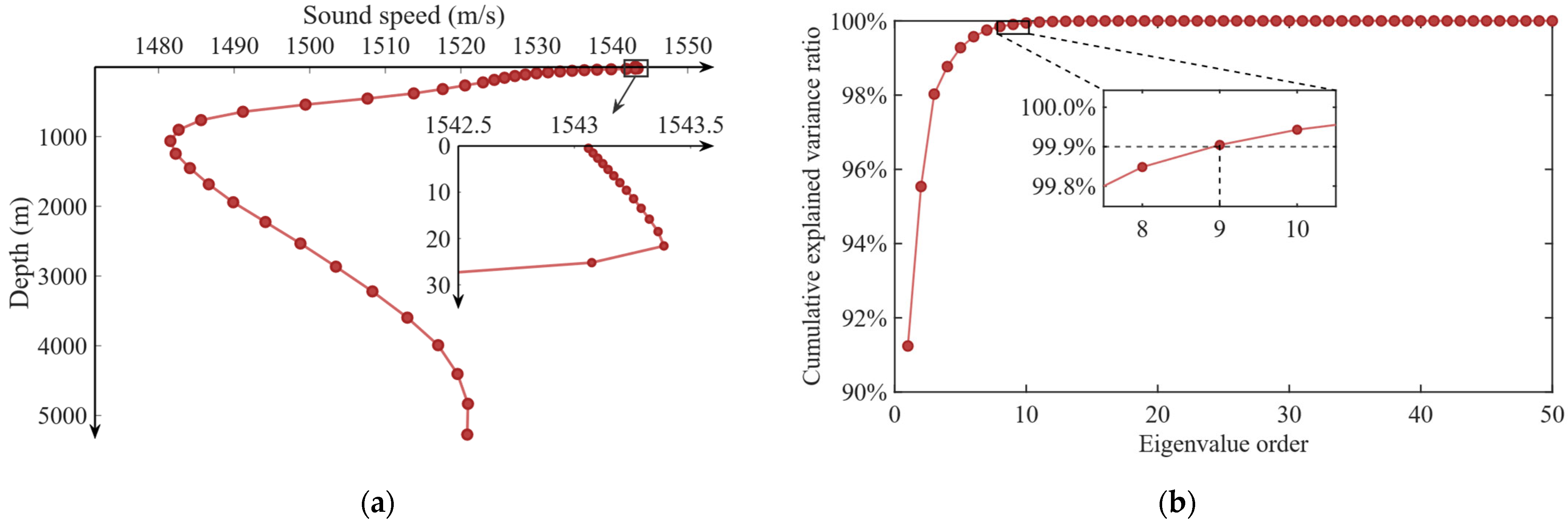
The threshold e_t in Section 3.2.2 is set to 99.9%, meaning that when the cumulative variance explained ratio is greater than or equal to 99.9%, the first k orthogonal empirical functions are considered to characterize the main features of seawater sound speed variations in the study area. Figure 2a shows the average SSP of the study area, and Figure 2b presents the curve of cumulative variance explained ratio versus eigenvalue order.

As observed in Figure 2a, the SSP of the study area consists of a surface layer, a main thermocline, and a deep isothermal layer. In the 0~25 m depth range, the sound speed exhibits a positive gradient distribution; a maximum value exists at 25 m depth; from 25~1000 m, the sound speed gradually decreases to a minimum; and from 1000 m to the seabed, the sound speed shows a positive gradient distribution. According to Figure 2b, the first 9 orders of EOF can be used to characterize the main features of seawater sound speed variations in the study area. Thus, the data dimension is reduced from the original 50 dimensions to 9 dimensions. Combined with longitude, latitude coordinates, and seabed elevation data, 12-dimensional data points are formed. There are 37 × 37 data points in the study area. To determine the optimal K value, K is iterated within the range [2,10], and the silhouette coefficient s is calculated, with results shown in

Table 1. Silhouette coefficients corresponding to different K values.

K Value	2	3	4	5	6	7	8	9	10
Silhouette coefficient s	0.2982	0.3141	0.3158	0.3432	0.3319	0.3331	0.3630	0.3396	0.3785

:

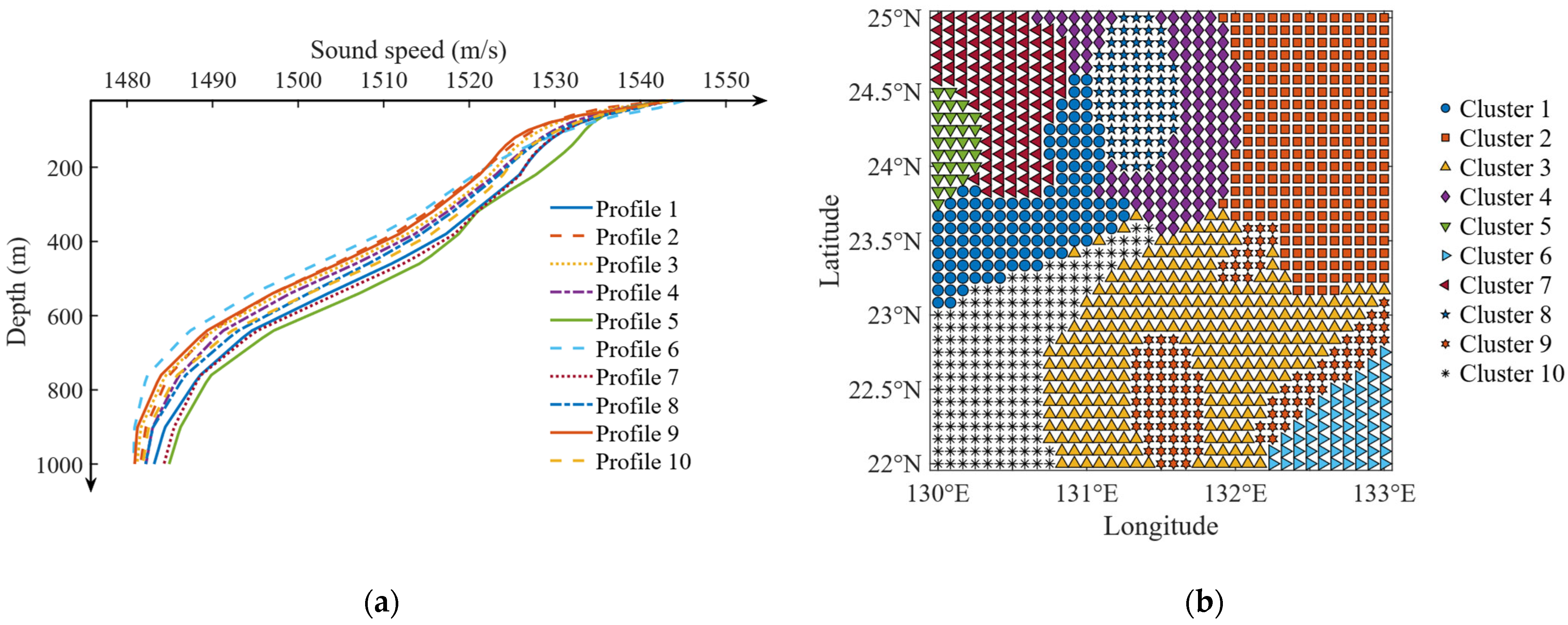
As indicated in Table 1, the optimal K value is 10. Thus, the K-means method is used to cluster the SSPs of the study area into 10 categories, with clustering results shown in Figure 3a,b and

Table 2. Coordinates of cluster centers.

Cluster	1	2	3	4	5	6	7	8	9	10
Latitude (° N)	23.71	24.16	22.79	24.35	24.15	22.25	24.50	24.50	22.63	22.71
Longitude (° E)	130.61	132.54	131.68	131.58	130.10	132.72	130.45	131.33	131.99	130.49

, respectively. Figure 3a displays the 10 types of average SSPs in the 20~1000 m depth range, Figure 3b shows the spatial distribution of the 10 types of data points, and Table 2 presents the central coordinates of data points in each cluster.

A comparison between Figure 2a and Figure 3a reveals that the sound speed variation trends of each category of SSPs in the 20~1000 m depth range are basically consistent with those of the average SSP, while there are certain differences in specific sound speed values, which is one of the main bases for clustering. Figure 3b indicates that the distribution of clustered data points has spatial correlation, which is closely related to the inclusion of geographical location information and seabed terrain information in the data points.

4.2. Sound Field Modeling Results

The operating frequency of the sonar used in this study is 15 kHz, which falls within the main frequency band of wind-generated noise. Therefore, the marine ambient noise level is primarily determined by wind-generated noise. Using the wind speed data at 10 m above the sea surface, the spatial distribution of NL in the study area is calculated as shown in Figure 4a. The NL in this area is approximately 40 dB, with the NL in the northeastern region being relatively small (less than 40 dB), while that in other regions is above 40 dB. The NL field affects the propagation of sound rays to a certain extent, thereby influencing the search distance of the sonar.

Based on the SSP clustering results, the study area is divided into 10 sub-regions. Within each sub-region, only the average SSP is considered, and combined with seabed terrain data (as shown in Figure 4b), the Bellhop model is used to solve the TL field. As shown in

Table 3. Comparison of computation time.

Clustering Applied	Time Consumption
Yes	10.84 min
No	24.74 h

, the computation time for the 10 clustered TL fields is 10.84 min, while calculating 37 × 37 TL fields one by one requires 24.74 h. Clustering significantly reduces the computation time of the sound field.

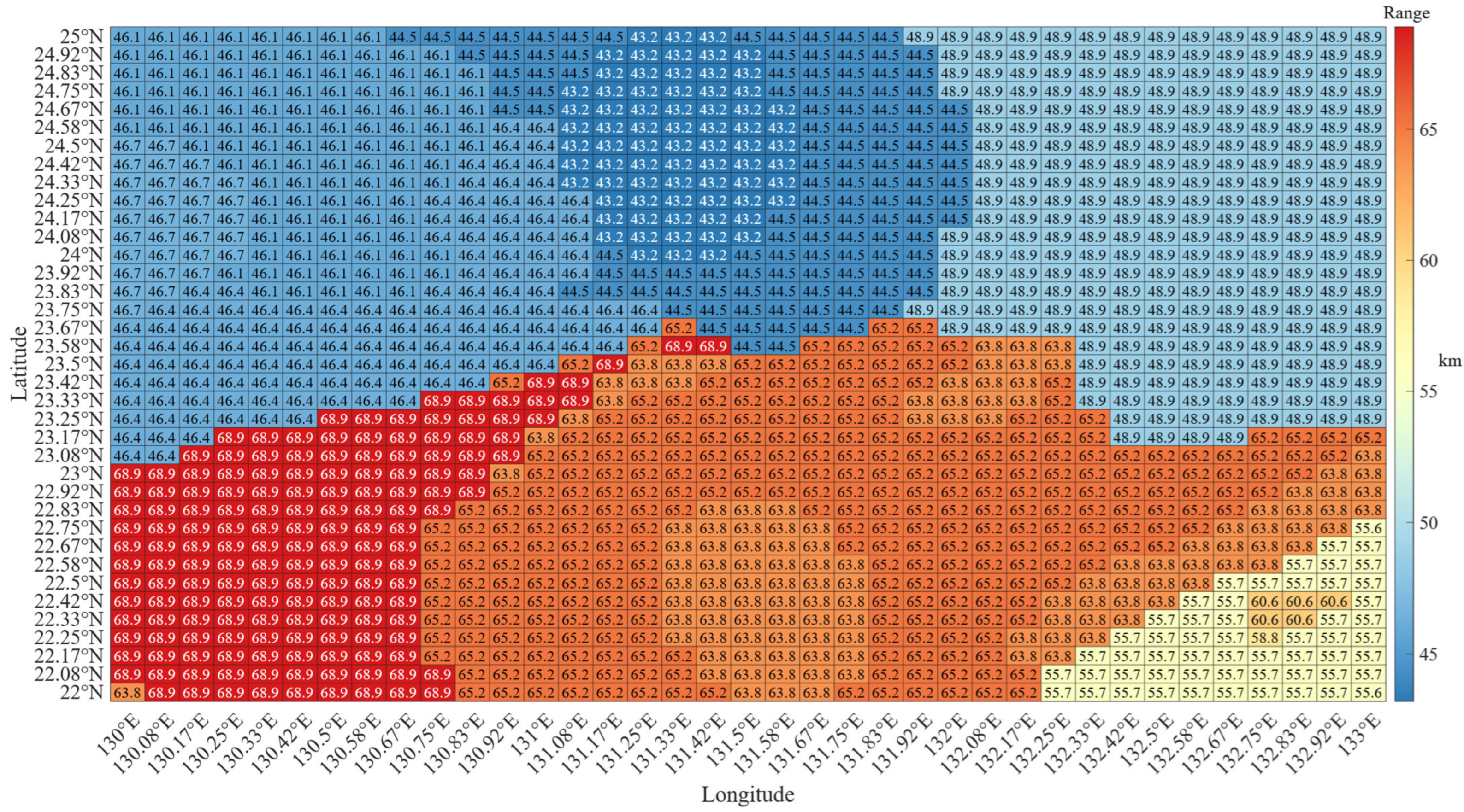
The spatial distribution of the sonar search distance is shown in Figure 5. A comparative analysis of Figure 3b, Figure 4a and Figure 5 reveals that the spatial distribution of the active sonar search distance in this area roughly corresponds to the spatial distribution of clustered data points but has little correlation with the distribution of NL. This indicates that the search distance of the active sonar in this area is mainly affected by the type of SSP.

4.3. Path Optimization Results

After solving the sonar search distance distribution, the IACO algorithm is introduced to optimize the search path. To ensure data reliability and avoid contingency, 50 groups of different initial paths are randomly generated according to the coding rules in Section 3.4.2, and each is optimized using the IACO algorithm. The parameter settings are as follows: initial pheromone concentration: 1; pheromone importance factor: 1; heuristic information importance factor: 4; basic evaporation rate: 0.2; pheromone increment constant: 100; elite proportion: 0.1.

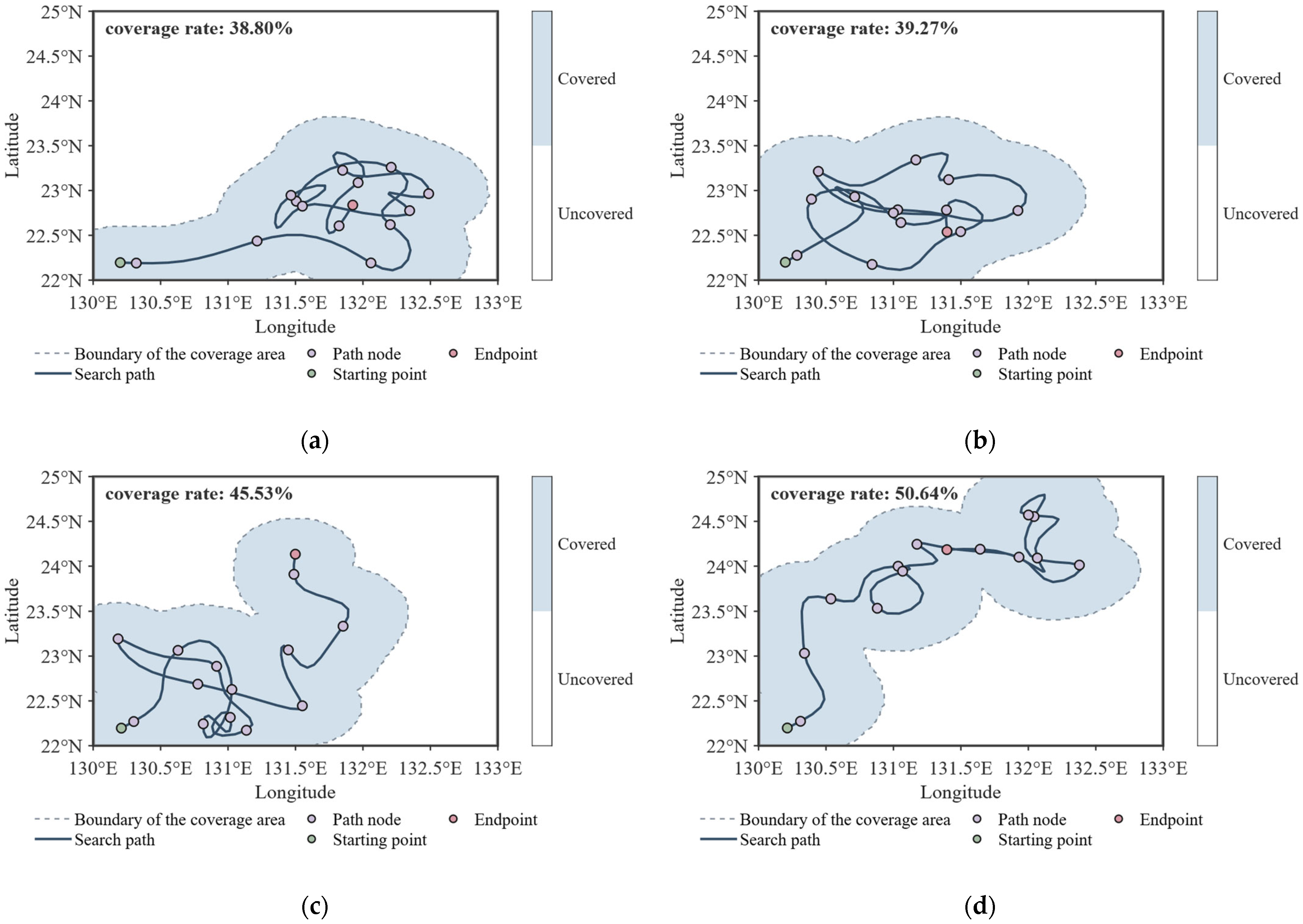
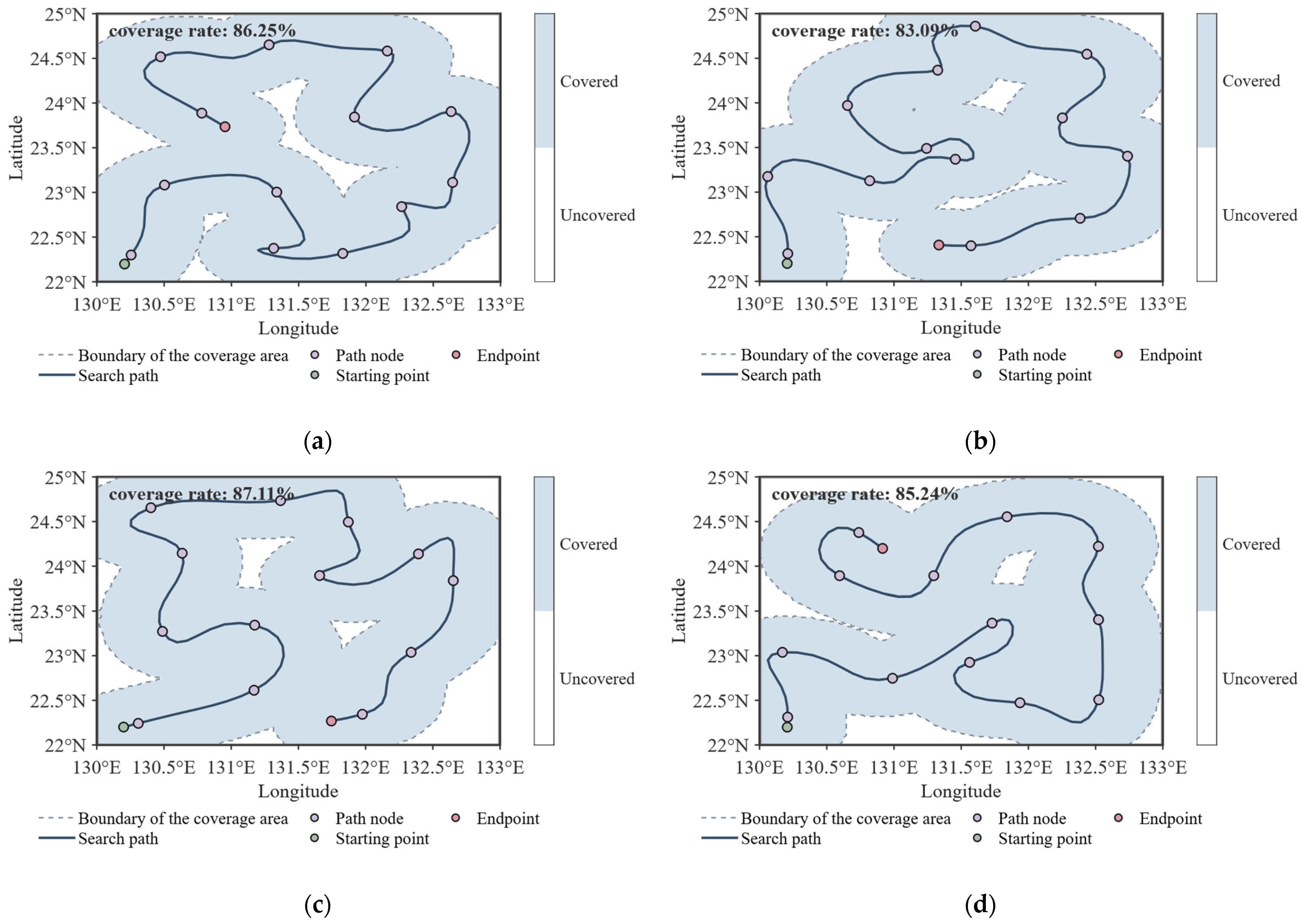
Figure 6 and Figure 7 illustrate the process as follows: The surface ship departs from the starting point and sails along the planned path. The blue area represents the coverage range of the sonar search, while the white area denotes the sonar detection blind zone. Since the target position information is unknown, it is assumed to be uniformly distributed. Thus, an optimal path needs to be planned to expand the search coverage as much as possible, so as to ensure the maximization of the target detection probability. Figure 6a–d show the first 4 groups of initial optimized paths, and Figure 7a–d present the optimal paths after 200 generations of iteration optimization by the IACO algorithm. The coverage rate in the figures refers to F(x_i) in Equation (30).

The average search coverage rate of the initial paths is 47.96%. After optimization by the IACO algorithm, the average search coverage rate reaches 86.01%, with an improvement of 79.34%. The initial paths have problems such as crossing, overlapping, frequent turns, and U-turns, resulting in low search coverage, which would cause fuel waste and steering gear wear in actual search processes. After iterative optimization, the search coverage rate is significantly improved, and the above problems are effectively solved.

4.4. Analysis of Optimization Algorithms

To verify the applicability and superiority of the designed IACO algorithm for this optimization problem, a comprehensive comparison is conducted with other advanced optimization algorithms, including GA, QPSO-TS, ISO, ADDE, and EDA. Fifty groups of populations are randomly generated, each containing 30 individuals, serving as the initial populations for all algorithms. The number of iterations is set to 200, and the uncoverage rate (1 − F(x_i)) is used as the evaluation index to plot convergence curves, with 50 independent repeated experiments performed for each algorithm.

4.4.1. Parameter Setting

To determine appropriate parameters, a pre-experiment was conducted prior to the formal experiment. The three most critical parameters in the IACO algorithm are the basic pheromone evaporation rate (ρ), pheromone importance factor (α), and heuristic information importance factor (β). Typically, the value range of ρ is 0.1–0.9, α is 1–5, and β is 2–10. Two of these parameters were kept constant while the third was varied within a reasonable range. Under the same initial population, 30 independent repeated experiments were performed. The average uncovered rate was used as the evaluation index to analyze the impact of parameter variations on the performance of IACO. The experimental results are shown in Figure 8a–c.

As indicated by the pre-experiment results, the optimal parameter settings are ρ = 0.2, α = 1, and β = 4. The parameter settings of other algorithms refer to Refs. [11,12], and the parameters of all algorithms are listed in

Table 4. Parameter settings of algorithms.

Algorithm	Parameter Values
IACO	Initial pheromone concentration: 1; Pheromone importance factor: 1; Heuristic information importance factor: 4; Basic evaporation rate: 0.2; Pheromone increment constant: 100; Elite proportion: 0.1
GA	Crossover probability: 0.5; Mutation probability: 1/N; Tournament selection size: 3; Elite retention ratio: 0.15
QPSO-TS	Contraction-expansion coefficient: 0.75; Tabu list length: 10; Tabu tenure: 5
ISO	Chaotic mapping parameter: 0.5; Dynamic weight factor: 1.2; Gaussian disturbance intensity: 0.2
ADDE	Initial mean of scaling factor: 0.5; Initial mean of crossover probability: 0.5; Elite proportion: 0.1
EDA	Minimum variable value: 1; Maximum variable value: 16; Retention proportion: 0.5

.

4.4.2. Performance Analysis

Figure 9a,b show the optimal convergence curves and average convergence curves of the six algorithms, respectively. The optimal convergence curve refers to the curve of the optimal fitness in the newly generated population varying with the number of iterations during each iteration. The average convergence curve refers to the curve of the non-zero fitness in the newly generated population varying with the number of iterations during each iteration process. As can be seen from Figure 9a, IACO exhibits the fastest convergence speed and the best optimization effect, while GA performs close to IACO. QPSO-TS, ISO, and ADDE show similar performance, with slower convergence speeds and inferior optimization effects compared to IACO and GA. EDA performs the worst, barely achieving any optimization. It can be observed from Figure 9b that the curves of IACO, ISO, ADDE, and EDA are relatively smooth, while those of GA and QPSO-TS fluctuate significantly. This is because GA and QPSO-TS generate more out-of-bound paths during iteration for new populations, resulting in a fitness of 0 and thus causing fluctuations in the average fitness.

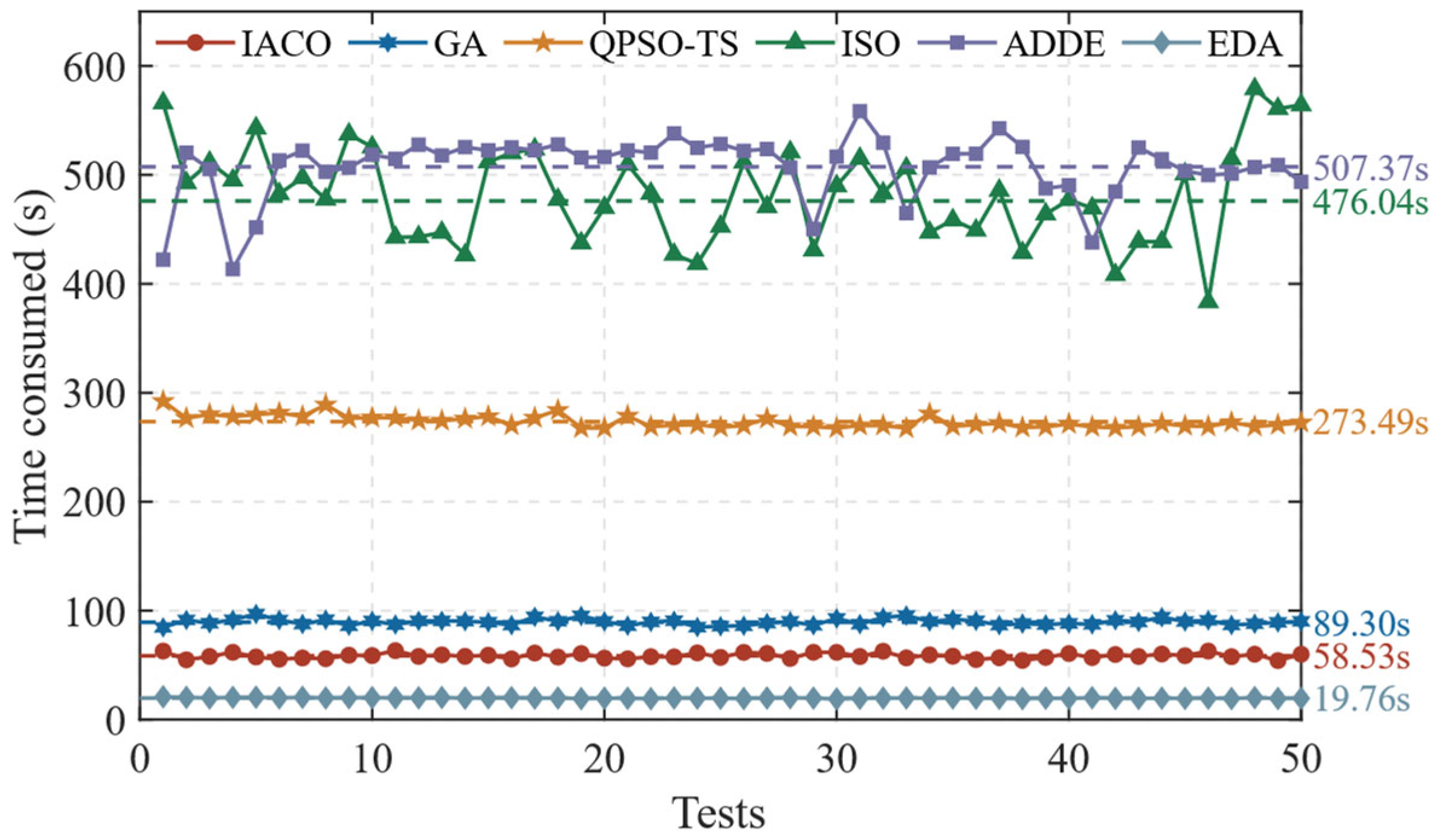
The time consumption of each algorithm in each test is statistically shown in Figure 10. The single optimization time consumption of IACO, GA, QPSO-TS, ISO, ADDE, and EDA is 58.53 s, 89.30 s, 273.49 s, 476.04 s, 507.37 s, and 19.76 s, respectively. Among them, EDA has the shortest single time consumption but the worst optimization effect, indicating that during iteration, it does not effectively approach the optimal solution but iterates repeatedly around inferior solutions. Except for EDA, IACO has the shortest single optimization time consumption, demonstrating that IACO is comprehensively superior to the other algorithms in performance.

The IACO algorithm is improved and designed specifically for the optimization problem of 16 discrete azimuth variables in this study, and it outperforms other algorithms in terms of convergence speed, computational efficiency, and optimization effect. The GA achieves an optimization effect close to that of IACO, but it generates more out-of-bound paths during iteration, thereby affecting its performance. QPSO-TS shows good performance in Ref. [12]; however, when the study sea area is expanded and the search step length is increased, it also suffers from the problem of generating more invalid populations, indicating that the robustness of this algorithm needs to be improved. The ISO algorithm is a gradient-based continuous optimization algorithm, which requires continuousization and subsequent discretization of discrete azimuths, resulting in the loss of solution accuracy. Although the ADDE algorithm adjusts parameters adaptively, its mutation operation is inefficient in discrete spaces. EDA is a static probability model that is difficult to reflect changes in path constraints in real time, with high resampling costs and the worst performance.

4.4.3. Statistical Significance Test

To conduct a more in-depth comparative study and determine whether there are significant differences in the final optimization effects between the IACO algorithm and the other five algorithms, non-parametric statistical tests were used for statistical analysis. The test samples were the search coverage rates of the six algorithms after 200 iterations of optimization, with a sample size of 50. Since the samples are independent and non-normally distributed data, the Wilcoxon signed-rank test was adopted. In essence, this test judges whether there are significant differences between two sets of related data by analyzing the signs and ranks of the data, and the results are shown in

Table 5. Wilcoxon signed-rank test results (compared with IACO).

Statistical Indicators	GA	QPSO-TS	ISO	ADDE	EDA
Rank sum statistic	2905.0	3701.5	3556.0	3687.0	3775.0
p-value	0.0089	5.1818 × 10−16	1.2113 × 10−12	1.1738 × 10−15	7.0661 × 10−18

.

As can be seen from Table 5, the p-values of the samples corresponding to IACO and GA, QPSO-TS, ISO, ADDE, and EDA are all less than 0.05, which allows us to reject the null hypothesis. It is determined that there are significant differences in the medians of the two sets of data, indicating that the optimization effect of IACO is significantly better than that of GA, QPSO-TS, ISO, ADDE, and EDA.

4.4.4. Computational Complexity Analysis

To comprehensively evaluate the performance of IACO and quantify the time cost, this study conducts a comparative analysis with benchmark algorithms from the perspective of computational complexity. The following section elaborates on the computational complexity of IACO, as well as GA, QPSO-TS, ISO, ADDE, and EDA, and compares the performance and computational cost of IACO.

Let the population size be M, the individual dimension be N, the number of iterations be I, and assume the computational complexity of the objective function is O(f). As indicated in Algorithm 1, the complexity of fitness calculation for IACO is O(M·f), the complexity of elite retention is O(M·logM), the complexity of individual construction is O(16M·N), and the complexity of pheromone update is O(M·N). Thus, the total complexity of IACO is O(I·(M·f + 16M·N + M·logM)). Similarly, the computational complexities of the other five benchmark algorithms can be derived, as shown in

Table 6. Comparison of computational complexities.

Algorithm	Computational Complexity
IACO	O(I·(M·f + 16M·N + M·logM))
GA	O(I·(M·f + 16M·N + M·logM))
QPSO-TS	O(I·(M·f + 16M·N + t·ns·N·f))
ISO	O(I·(M·f + 16M·N + M·logM))
ADDE	O(I·(M·f + 16M·N + M·logM))
EDA	O(I·(M·f + 16M·N))

.

In Table 6, t denotes the tabu tenure of the QPSO-TS algorithm, and ns represents the neighborhood size of tabu search in the QPSO-TS algorithm. As can be seen from Table 6, the dominant complexity of all algorithms is O(I·(M·f + 16M·N)). Since the objective function in this study is relatively simple, the term 16M·N becomes the dominant factor, so the dominant complexity is simplified to O(16I·M·N)). The differences mainly lie in the constant factors and low-level operations. The computational complexities of the six algorithms are not significantly different, and the computational cost per iteration is similar. However, the IACO algorithm has advantages in the final optimization effect, convergence speed, and optimization time consumption. Therefore, the performance improvement of the IACO algorithm outweighs its potential computational cost.

5. Conclusions

To address the issue of low efficiency in underwater acoustic modeling for surface ship path planning in underwater target search, this study proposes an efficient underwater target search path planning method based on SSP clustering, and its effectiveness is verified through numerical simulations. The main conclusions are as follows:

First, the path planning for underwater target search is affected by the marine acoustic environment. Environmental factors such as the spatial distribution of seawater temperature, salinity, and pressure, sea surface wind speed, ship noise, seabed topography, and seabed sediment all influence the detection range of sonar, thereby affecting the results of path planning.

Second, the introduction of SSP clustering effectively improves the efficiency of underwater acoustic modeling. By utilizing the spatial correlation of acoustic environments in adjacent sea areas to simplify underwater acoustic modeling, it effectively addresses the issue of significant computational time consumption caused by considering SSPs of all sampling points and also avoids the loss of accuracy due to simple averaging.

Third, the IACO algorithm exhibits excellent performance in path optimization. Essentially, the path planning in this study belongs to a discrete optimization problem with integer coding. The IACO algorithm designed for this problem has advantages in terms of convergence speed, optimization effect, and computational efficiency.

However, two aspects of limitations should be noted. Firstly, the sound speed clustering method proposed in this paper is developed based on deep-sea areas. In shallow-sea environments, environmental factors such as SSPs and topography exhibit more drastic spatiotemporal variations, which may lead to a larger number of clusters. Thus, a balance between computational efficiency and clustering granularity needs to be maintained. Secondly, the underwater acoustic field modeling is based on a specific target depth. This paper takes a water depth of 200 m as a case study to verify the feasibility of the proposed method, while the depth dimension of underwater targets can be further expanded.

As future work, it may be meaningful to consider ocean reverberation and shallow-sea environments, as shipping activities in shallow seas are generally more intensive than those in deep seas. Another direction for future research is to apply parallel computing technology to underwater acoustic field calculation to improve the computation speed of the underwater acoustic field. Finally, autonomous target search path planning for underwater unmanned vehicles may be a promising research direction.

References

1. Qian, L.; Li, H.; Wang, H.; Hong, M.; Han, J. Underwater target search and placement strategies based on an improved hidden Markov model. Sci. Sin. Technol. 2025, 55, 520–539. [Google Scholar] [CrossRef]
2. Urick, R.J. Principles of Underwater Sound, 3rd ed.; McGraw-Hill: New York, NY, USA, 1983; pp. 1–425. ISBN 9780070660878. [Google Scholar]
3. Wu, Y.; Su, X.; Cui, J.; Yang, G. Coordinated path planning of USV&AUV for an underwater target. Control. Decis. 2021, 36, 825–834. [Google Scholar] [CrossRef]
4. Hamilton, E.L. Geoacoustic modeling of the sea floor. J. Acoust. Soc. Am. 1980, 68, 1313–1340. [Google Scholar] [CrossRef]
5. Li, J.; Johnson-Roberson, M. Multi-altitude multi-sensor fusion framework for AUV exploration and survey. In Proceedings of the 2014 Oceans-St. John’s, St. John’s, NL, Canada, 14–19 September 2014; pp. 1–8. [Google Scholar] [CrossRef]
6. Medwin, H.; Clay, C.S. Fundamentals of Acoustical Oceanography; Academic Press: New York, NY, USA, 1998; pp. 1–712. ISBN 978-0-12-487570-8. [Google Scholar]
7. Oliveira, T.C.A.; Lin, Y.T.; Porter, M.B. Underwater Sound Propagation Modeling in a Complex Shallow Water Environment. Front. Mar. Sci. 2021, 8, 751327. [Google Scholar] [CrossRef]
8. Yu, F.; Shang, H.; Zhu, Q. An efficient RRT-based motion planning algorithm for autonomous underwater vehicles under cylindrical sampling constraints. Auton. Robot. 2023, 47, 281–297. [Google Scholar] [CrossRef]
9. Ren, Y.; Zhang, L. An Adaptive Evolutionary Multi-Objective Estimation of Distribution Algorithm and Its Application to Multi-UAV Path Planning. IEEE Access 2023, 11, 50038–50051. [Google Scholar] [CrossRef]
10. Ai, B.; Jia, M.; Xu, H.; Xu, J.; Wen, Z.; Li, B.; Zhang, D. Coverage path planning for maritime search and rescue using reinforcement learning. Ocean Eng. 2021, 241, 110098. [Google Scholar] [CrossRef]
11. Liao, S.; Xiao, W.; Wang, Y. Optimization of route planning based on active towed array sonar for underwater search and rescue. Ocean Eng. 2025, 330, 121249. [Google Scholar] [CrossRef]
12. Wang, W.; Xiao, W.; Liu, Y. Research on Path Optimization for Underwater Target Search Under the Constraint of Sea Surface Wind Field. J. Mar. Sci. Eng. 2025, 13, 1393. [Google Scholar] [CrossRef]
13. Tang, Y.; Zhou, Q.; Wang, X.; Xie, Z. A Computational Method for Acoustic Interaction with Large Complicated Underwater Structures Based on the Physical Mechanism of Structural Acoustics. Adv. Mater. Sci. Eng. 2022, 2022, 3631241. [Google Scholar] [CrossRef]
14. Xu, X.; Liu, W.; Xu, G. A Time-Domain Wavenumber Integration Model for Underwater Acoustics Based on the High-Order Finite Difference Method. J. Mar. Sci. Eng. 2024, 12, 728. [Google Scholar] [CrossRef]
15. Jensen, F.B.; Kuperman, W.A.; Porter, M.B.; Schmidt, H. Computational Ocean Acoustics, 2nd ed.; Springer: Berlin/Heidelberg, Germany, 2011; pp. 377–452. ISBN 978-1-4419-8677-1. [Google Scholar]
16. Mackenzie, K.V. Nine-term equation for sound speed in the oceans. J. Acoust. Soc. Am. 1981, 70, 807–812. [Google Scholar] [CrossRef]
17. Tobler, W.R. A Computer Movie Simulating Urban Growth in the Detroit Region. Econ. Geogr. 1970, 46, 234–240. [Google Scholar] [CrossRef]
18. Zhang, Z.; Qu, K.; Li, Z. An Enhanced Approach for Sound Speed Profiles Inversion Using Remote Sensing Data: Sample Clustering and Physical Regression. Electronics 2025, 14, 2822. [Google Scholar] [CrossRef]
19. Li, Q.; Zhu, J.; Luo, Y.; Peng, D. Reconstruction Performance Analysis for Basis Function of the Sound Speed Profile. Acta Oceanol. Sin. 2023, 45, 34–44. [Google Scholar] [CrossRef]
20. Huang, W.; Wu, P.; Lu, J.; Lu, J.; Xiu, Z.; Xu, Z.; Li, S.; Xu, T. Underwater SSP Measurement and Estimation: A Survey. J. Mar. Sci. Eng. 2024, 12, 2356. [Google Scholar] [CrossRef]
21. Li, B.; Zhai, J. A Novel Sound Speed Profile Prediction Method Based on the Convolutional Long-Short Term Memory Network. J. Mar. Sci. Eng. 2022, 10, 572. [Google Scholar] [CrossRef]
22. Liu, Y.; Chen, W.; Chen, W.; Chen, Y.; Ma, L.; Meng, Z. Reconstruction of Ocean Front Model Based on Sound Speed Clustering and Its Effectiveness in Ocean Acoustic Forecasting. Appl. Sci. 2021, 11, 8461. [Google Scholar] [CrossRef]
23. Ballard, M.S. Clustering Analysis of a Yearlong Record of Ambient Sound on the Chukchi Shelf in the 40 Hz to 4 kHz Frequency Range. J. Acoust. Soc. Am. 2021, 150, 1597–1608. [Google Scholar] [CrossRef] [PubMed]
24. Li, Q.; Han, X.; Wei, L.; Cao, R.; Wei, Z. Depth discrimination of passive sources in the Beaufort Sea of the Arctic. Acta Acust. 2025, 50, 665–676. [Google Scholar] [CrossRef]
25. Zhang, L.; Ge, Y.; Guan, Z.; Ye, G.; Feng, H. Path planning of underwater vehicle based on improved particle swarm algorithm. In Proceedings of the 2024 36th Chinese Control and Decision Conference, Xi’an, China, 25–27 May 2024; pp. 5584–5589. [Google Scholar] [CrossRef]
26. Liu, Y.; Wu, A. AUV Path Planning Based on Improved Ant Colony Algorithm. In Proceedings of the 2nd International Conference on Artificial Intelligence, Robotics, and Communication, Fuzhou, China, 25–27 November 2023; Volume 1063. [Google Scholar] [CrossRef]
27. Orozco-Rosas, U.; Montiel, O.; Sepúlveda, R. Mobile robot path planning using membrane evolutionary artificial potential field. Appl. Soft Comput. 2019, 77, 236–251. [Google Scholar] [CrossRef]
28. Orozco-Rosas, U.; Picos, K.; Pantrigo, J.J.; Montemayor, A.S.; Cuesta-Infante, A. Mobile Robot Path Planning Using a QAPF Learning Algorithm for Known and Unknown Environments. IEEE Access 2022, 10, 84648–84663. [Google Scholar] [CrossRef]
29. Wang, Y.; Liu, K.; Geng, L.; Zhang, S. Knowledge hierarchy-based dynamic multi-objective optimization method for AUV path planning in cooperative search missions. Ocean Eng. 2024, 312, 119267. [Google Scholar] [CrossRef]
30. Tang, Z.; Cao, X.; Zhou, Z.; Zhang, Z.; Xu, C.; Dou, J. Path planning of autonomous underwater vehicle in unknown environment based on improved deep reinforcement learning. Ocean Eng. 2024, 301, 117547. [Google Scholar] [CrossRef]
31. Millero, F.J.; Li, X. On equations for the speed of sound in seawater-comment. J. Acoust. Soc. Am. 1994, 95, 2757–2759. [Google Scholar] [CrossRef]
32. Leroy, C.C.; Parthiot, F. Depth-pressure relationships in the oceans and seas. J. Acoust. Soc. Am. 1998, 103, 1346–1352. [Google Scholar] [CrossRef]
33. Hu, J.; Xiao, Y.; Zhang, D.; Leng, L. Inversion Prediction Method for Sound Speed Profile. Adv. Mar. Sci. 2019, 37, 245–254. [Google Scholar] [CrossRef]
34. Rousseeuw, P.J. Silhouettes: A graphical aid to the interpretation and validation of cluster analysis. J. Comput. Appl. Math. 1987, 20, 53–65. [Google Scholar] [CrossRef]
35. Munk, W.; Snodgrass, F.; Caiiier, G. Edge Waves on the Continental Shelf. Science 1956, 123, 127–132. [Google Scholar] [CrossRef]
36. Woezel, J.L.; Ewing, M.; Pekeris, C.L. Propagation of Sound in the Ocean. In Geological Society of America Memoirs; Geological Society of America: Boulder, CO, USA, 1948; Volume 27, pp. 1–62. [Google Scholar] [CrossRef]
37. Tappert, F.D. The parabolic approximation method. In Wave Propagation and Underwater Acoustics; Springer: Berlin/Heidelberg, Germany, 1977; Volume 70, pp. 224–287. [Google Scholar] [CrossRef]
38. Xi, Q.; Fu, Z.; Xu, W.; Xue, M.; Rashed, Y.F.; Zheng, J. FEM-PIKFNN for underwater acoustic propagation induced by structural vibrations in different ocean environments. Comput. Math. Appl. 2024, 176, 46–54. [Google Scholar] [CrossRef]
39. Liao, S.; Xiao, W.; Wang, Y. Dynamic hybrid parallel computing of the Ray Model for solving underwater acoustic fields in vast sea. Sci. Rep. 2024, 14, 25385. [Google Scholar] [CrossRef] [PubMed]
40. Wenz, G.M. Acoustic ambient noise in the ocean: Speactra and source. J. Acoust. Soc. Am. 1962, 34, 1936–1956. [Google Scholar] [CrossRef]
41. Kularia, Y.; Bhattacharya, P. Analysis of Acoustic Channel Characteristics for Underwater Wireless Sensor Networks. Int. J. Comput. Sci. Inf. Technol. Control. Eng. 2016, 3, 11–24. [Google Scholar] [CrossRef]
42. Harrison, C.H. Noise directionality for surface sources in range-dependent environments. J. Acoust. Soc. Am. 1997, 102, 2655–2662. [Google Scholar] [CrossRef]
43. Xu, L.; Cao, M.; Song, B. A new approach to smooth path planning of mobile robot based on quartic Bezier transition curve and improved PSO algorithm. Neurocomputing 2022, 473, 98–106. [Google Scholar] [CrossRef]
44. Hu, H.; Zhang, Z.; Wang, T.; Peng, X. Underwater glider 3D path planning with adaptive segments and optimal motion parameters based on improved JADE algorithm. Ocean Eng. 2024, 299, 117377. [Google Scholar] [CrossRef]
45. Yang, P.; Tang, K.; Lozano, J.A. Estimation of Distribution Algorithms based Unmanned Aerial Vehicle path planner using a new coordinate system. In Proceedings of the 2014 IEEE Congress on Evolutionary Computation, Beijing, China, 6–11 July 2014; pp. 1469–1476. [Google Scholar] [CrossRef]
46. Huang, S.; Yang, D.; Zhong, C.; Yan, S.; Zhang, L. An Improved Ant Colony Optimization Algorithm for Multi-Agent Path Planning. In Proceedings of the 2021 International Conference on Networking Systems of AI, Shanghai, China, 19–20 November 2021; pp. 95–100. [Google Scholar] [CrossRef]
Figure 1. Study area.
Jmse 13 01983 g001
Figure 2. Results of EOF decomposition. (a) Average SSP; (b) Curve of cumulative variance explained ratio.
Jmse 13 01983 g002
Figure 3. Clustering results. (a) SSP clustering results; (b) Spatial distribution of clustered data points.
Jmse 13 01983 g003
Figure 4. Acoustic environment. (a) NL field; (b) Seabed terrain.
Jmse 13 01983 g004
Figure 5. Spatial distribution of active sonar search distance.
Jmse 13 01983 g005
Figure 6. Initial planned paths. (a) Initial path 1; (b) Initial path 2; (c) Initial path3; (d) Initial path 4.
Jmse 13 01983 g006
Figure 7. Optimal paths. (a) Optimal path 1; (b) Optimal path 2; (c) Optimal path3; (d) Optimal path 4.
Jmse 13 01983 g007
Figure 8. Pre-experiment results. (a) Basic pheromone evaporation rate; (b) Pheromone importance factor; (c) Heuristic information importance factor.
Jmse 13 01983 g008
Figure 9. Convergence curves. (a) Optimal convergence curve; (b) Average convergence curve.
Jmse 13 01983 g009
Figure 10. Optimization time consumption.
Jmse 13 01983 g010