Long-Term Significant Wave Height Forecasting in the Western Atlantic Ocean Using Deep Learning

Abstract

This study presents a significant wave height correction model using deep learning techniques to enhance long-term wave forecast capabilities. The model utilises buoy measurements to assess the forecasting accuracy of the ECMWF 15-day forecast of significant wave height in the western Atlantic Ocean under various input conditions. The performance of different deep learning methods in modelling the wave forecast error is compared. The model predictions are validated against buoy data, revealing that the forecasting accuracy of the various deep learning methods is comparable. In addition, the model’s adaptability is examined for varying locations and water depths within the study area. The results demonstrate that the proposed method significantly improves the accuracy of the 15-day wave height forecasting and exhibits good adaptability to a vast sea area.

1. Introduction

Waves, as a vital component of the oceanic dynamical system, hold significant research importance in the context of global climate change and maritime navigation. Accurate wave modelling contributes to enhanced climate models by improving the simulation and prediction of ocean surface energy transfer and the impact of wind waves on climate patterns. Furthermore, it enhances the safety of maritime transportation and reduces the incidence of accidents caused by adverse sea conditions. Specifically, long-term wave forecasting provides a more reliable basis for planning maritime navigation [1], allowing advance time for the early prevention of extreme weather events and the avoidance of bad weather by ships [2]. Thus, research on long-term wave forecasting holds significant scientific and practical importance.

Numerical models represent one of the core methodologies in the current field of ocean forecasting. By solving the dynamical equations that describe wave generation, propagation, and dissipation, these models can achieve the projection of sea states on both global and regional scales. Typically, these models incorporate atmospheric forcing data such as wind speed and direction, along with initial conditions of the marine environment, to simulate the evolution of wave patterns over a specified future period. Typical numerical models such as WAM [3], WAVEWATCH III [4], and SWAN [5] are widely applied. These numerical models, which have been improved with time with additional formulations, provide relatively accurate short-term and medium-term results, demonstrating significant advantages, particularly in wind wave fields and wave propagation. A comparison of different hindcast databases produced by these models reveals that, except for extreme values, the predictions are highly consistent [6].

However, the forecasting accuracy of numerical models relies on the input meteorological data [7,8,9,10] and physical parameterisation schemes, with uncertainty increasing as the forecast period extends. Additionally, numerical models typically require solving complex dynamical equations that involve multiple source terms, boundary conditions, and nonlinear processes, resulting in substantial computational demand.

The computational time increases significantly in forecasts over large spatial scales or extended time frames. Computational efficiency constrains the application of numerical models, which are still widely used in environmental forecasting and hindcasting [11,12,13,14,15].

While in the hindcast mode, the wave fields are obtained by wind fields updated at each time step from a historical database, in the forecast mode, the evolution of the wind fields that will force the wave model is itself a result of numerical models. This implies that the skill of the models deteriorates as the forecast time increases, a feature that has been well known for a long time. Presently, forecasts are routinely made for periods of 10 to 15 days, but they only show excellent skill for periods of around four days. Therefore, various authors have been attempting to utilise different types of artificial intelligence models to enhance the results of physical models for horizons of 10 to 15 days.

Campos and Guedes Soares [16] have proposed the approach of combining the traditional numerical wave model with a statistically based model to improve it, a methodology that they applied in various subsequent publications. Campos et al. [17] used Random Forest models to enhance wave forecasting by selecting the more accurate forecast between a deterministic forecast and the mean of an ensemble of forecasts. They concluded that Random Forest models perform well for short-term predictions, but their accuracy was reduced for forecasts beyond five days due to increased uncertainty associated with the ensemble spread.

Costa et al. [18] chose the multilayer perceptron and a Long Short-Term Memory (LTSM) neural network to improve the accuracy of ERA5 hourly data of 10 m wind speed and significant wave height at two locations of the western Atlantic Ocean with distinct metocean conditions. They concluded that the LTSM was the one that obtained the best results. Then, the LSTM model was also applied by Henriques and Guedes Soares [19] to enhance the predictions of an in-house wave forecast model in the eastern Atlantic, utilising buoy data located near the Iberian Peninsula. The corrections focused on the significant wave height and peak period, but the best results were obtained for the former.

Yanchin and Guedes Soares [20] employed gradient-boosted trees, which are multi-output models that can simultaneously improve significant wave height and wind speed forecasts. They calculate the residue between the model’s results and the actual buoy observations, which can then be used to correct the prediction results. They also considered the residue to be noisy and used a denoising autoencoder to improve the forecast. Good results were obtained for wind forecasts, but the improvements in wave forecasts were modest.

With the accumulation of vast marine observational data and the enhancement of computational capabilities, deep learning models have emerged as practical tools for addressing complex nonlinear forecasting problems. Compared to traditional numerical models, deep learning can extract high-dimensional features from data, offering strong predictive power. In marine environmental forecasting, deep learning has already been applied in studies related to wave predictions [21,22,23], sea surface temperature [24,25,26], and ocean circulation [27]. Zhang et al. [28] developed a forecasting model based on deep learning methods for sea surface current and elevation. The model achieves high-accuracy predictions of marine environments by incorporating physical mechanisms and assigning greater weight to higher-magnitude flow velocities.

Additionally, deep learning is used for multi-source data fusion, enabling the integration of satellite, buoy, radar, and numerical model outputs to optimise further forecasting results [29]. Atteia et al. [30] proposed a novel hybrid feature selection method based on deep learning for forecasting significant wave height using Synthetic Aperture Radar (SAR) altimetry data from satellites. The study uses SAR mode data from the Sentinel-3A satellite and calibrates it with field buoy data to enhance prediction accuracy.

Researchers have conducted relevant studies on wave height forecasting. Bekiryazıcı et al. [31] developed an innovative deep learning method that combines Variational Mode Decomposition (VMD), Long Short-Term Memory (LSTM), and Transfer Learning for forecasting significant wave height over the next 36 h. The model’s accuracy was evaluated using various metrics. Ultimately, compared to the ECMWF IFS, the proposed model demonstrated a higher correlation with observed wave heights and the lowest error. Halicki et al. [32] used an Artificial Neural Network (ANN) for short-term significant wave height forecasting and rigorously optimised the model parameters to enhance accuracy. The study ultimately found that the developed model can accurately predict wave heights across various forecasting ranges. In recent years, deep learning methods have been widely applied in wave forecasting research [33,34].

With their strong data feature extraction capabilities, deep learning methods can enhance the efficiency of traditional numerical computation methods in predicting sea states. However, existing deep learning-based environmental forecasting research primarily focuses on short-term forecasts. In particular, wave forecasting can achieve high accuracy for 12 h to 3 days [17,20]. However, research on long-term forecasting remains limited. The involvement of additional uncertainty factors in long-term forecasting reveals the complexity of the oceanic and atmospheric systems over extended time frames. Traditional deep learning models face challenges in addressing these nonlinear dynamic processes.

The present study focuses on forecasting Hs over long time scales, introducing the Wave Forecast Artificial Intelligence (WF-AI) model using deep learning techniques. The model predicts Hs for the next 15 days using buoy measurements and wave forecast data provided by ECMWF. The performance of this and other forecast data has been evaluated through comparisons with multiple wave buoys and satellite data, particularly in the western Atlantic Ocean. Furthermore, this research compares the forecasting performance of various deep learning methods for wave predictions, including Artificial Neural Networks (ANNs), Recurrent Neural Networks (RNNs), Long Short-Term Memory (LSTM) networks, and the Transformer model. Ultimately, high-accuracy forecasts of Hs for the eastern United States coastal waters over extended periods are achieved.

The organisation of this paper is as follows: Section 2 introduces the study area and the data used. Section 3 presents the wave forecasting methods and deep learning models used in this study. Section 4 analyses the forecasting accuracy of the models, discussing their performance in predicting Hs for 1-, 3-, 6-, 10-, 12-, and 15-day forecasts. Additionally, the adaptability of the models is examined. Section 5 concludes the work presented in this paper.

2. Study Area and Data

The western Atlantic Ocean is selected as the study area in this study. This area experiences significant seasonal variations in wave characteristics due to the influences of storms and ocean currents, resulting in a rich energy profile. Particularly during the autumn and winter seasons, wave heights are notably increased, mainly due to the impact of Atlantic hurricanes and winter storms. The waves generated by these storms possess substantial energy and can propagate over long distances.

The Gulf Current passes through this general area, and the interaction of the waves with the current will affect their height. The standard wave models do not operationally model this interaction; thus, the simple presence of currents creates discrepancies between the predicted and measured heights.

The area is adjacent to the continent, resulting in considerable variations in water depth. While the open ocean is often affected by long-period swells generated by distant storms, the nearshore region is more influenced by local wind fields, exhibiting characteristics of short-period waves.

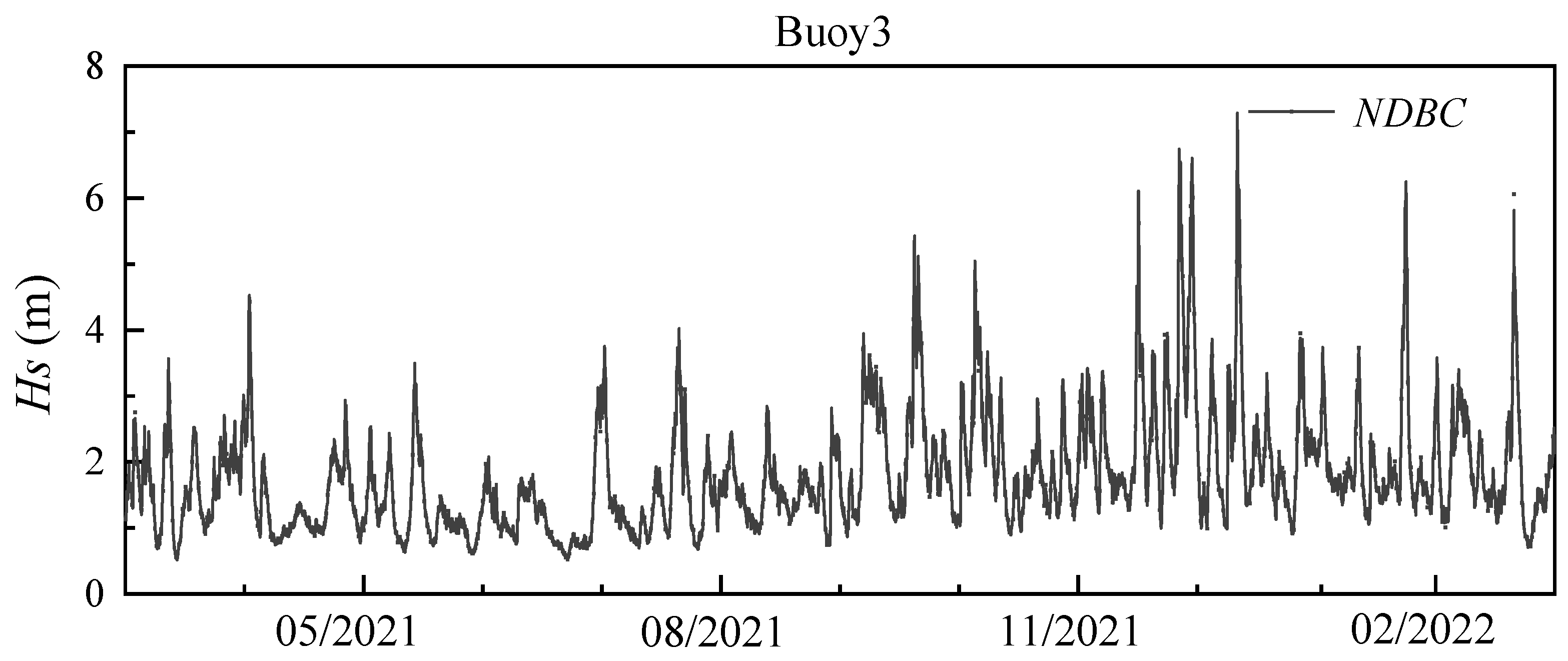
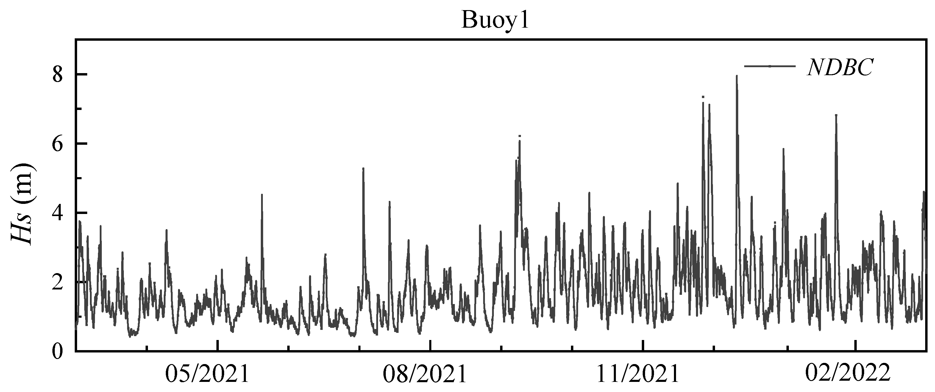
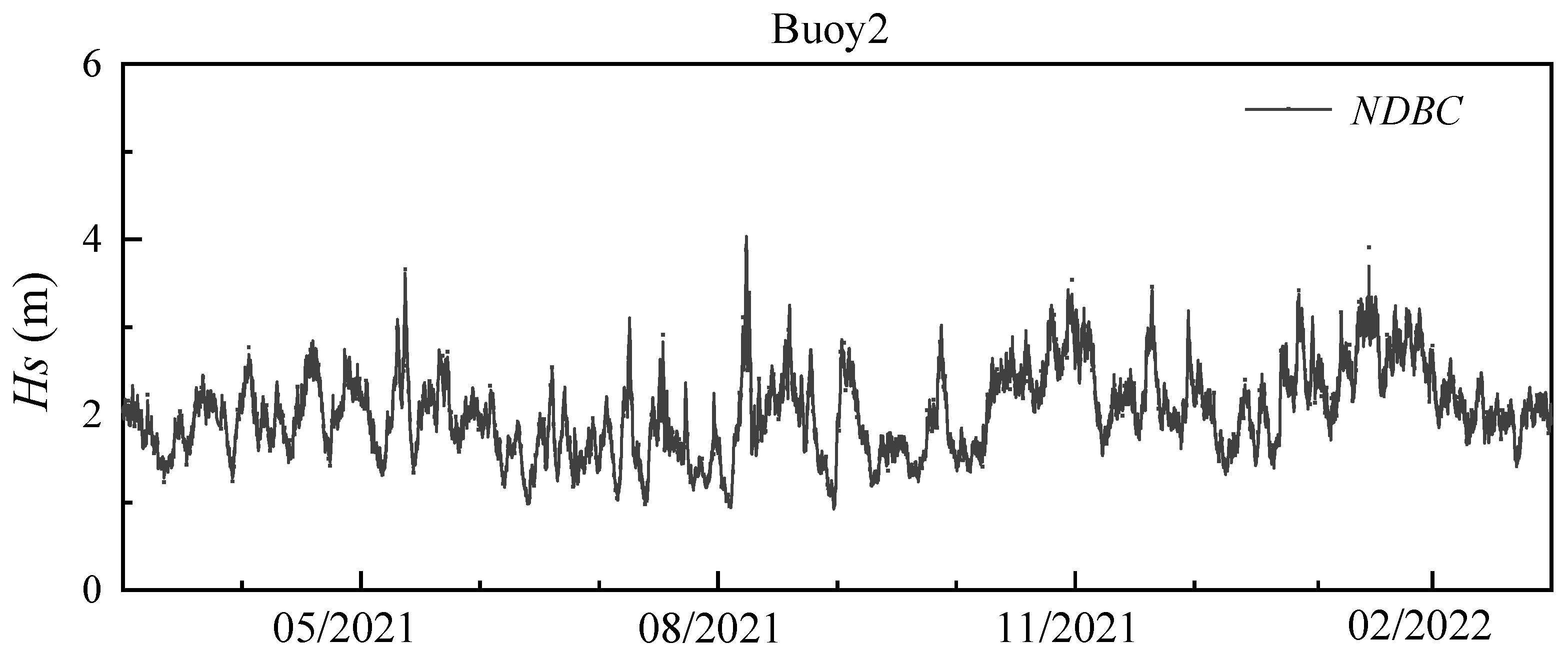
This study uses wave data from the National Data Buoy Center (NDBC). For the eastern United States coastal waters, three buoys are selected for analysis: Buoy 1 (44008), Buoy 2 (41040), and Buoy 3 (41048). Detailed information is provided in Figure 1 and Table 1. To comprehensively evaluate the model performance, buoy locations with varying water depths are selected within the study area. Buoy 1 is close to the mainland and has shallow water depths. At the same time, Buoys 2 and 3 are located in the open sea, at a considerable distance from the mainland, with water depths of approximately 5000 m. The NDBC records hourly or half-hourly wave measurements at each buoy location, totalling over 8000 wave data entries throughout the year. The wave data collected spans from April 2021 to March 2022, with specific conditions at the three buoy locations illustrated in Figure 2, Figure 3 and Figure 4. The wave height variations indicate that at Buoy 1, the sea conditions are relatively calm in spring and summer, with wave heights around 1.5 m, while rougher conditions occur in autumn and winter, with an average wave height of 2–3 m and a maximum reaching 8 m. At Buoy 2, wave heights remain at 2–3 m throughout the year. At Buoy 3, rougher sea conditions are also observed in autumn and winter.

Figure 1. Study area schematic diagram.

Table 1. Location information of selected buoys.

No.	Buoy	Lat	Lon	Depth
1	44008	40.496° N	69.250° W	72 m
2	41040	14.536° N	53.136° W	4988 m
3	41048	31.831° N	69.573° W	5394 m

Figure 2. Time series of Hs for Buoy 44008.

Figure 3. Time series of Hs for Buoy 41040.

Figure 4. Time series of Hs for Buoy 41048.

Additionally, wave forecast data are utilised in this study. The Ensemble Forecast [35] data are obtained from the European Centre for Medium-Range Weather Forecasts (ECMWF) operational prediction system. The atmospheric ensemble, known as the Ensemble Forecast (ENFO), is based on the Integrated Forecasting System (IFS) [36] and consists of 51 members (one control and 50 perturbed runs). The Wave Ensemble Forecast (WAEF) is produced using the third-generation WAM model [37], driven by 10 m winds from ENFO, and employs the same ensemble configuration and forecast length. Both ENFO and WAEF provide forecasts up to 15 days, with temporal output available hourly up to 90 h, every 3 h from 90 to 144 h (93–144 h for ENFO), and every 6 h from 150 to 360 h. For this study, data from the 00 UTC cycle were retrieved for all ensemble members and forecast lead times. The atmospheric data (wind parameters) were downloaded on a 0.20° × 0.20° regular latitude–longitude grid, while wave parameters (significant wave height (SWH)) were downloaded on a 0.25° × 0.25° grid. These resolutions correspond to interpolated output from ECMWF’s native model grids (≈9 km for both ENFO and WAEF), as provided by the MARS archive. Wind and wave forecast data corresponding to three buoy locations are obtained for the period from April 2021 to March 2022. The specific dimensions of the data are 145 × 365 × 3. Among them, 145 represents the forecast lead time in days, 365 corresponds to the daily updates over a year, and 3 denotes the number of variables.

3. Methodology

3.1. The WF-AI Model

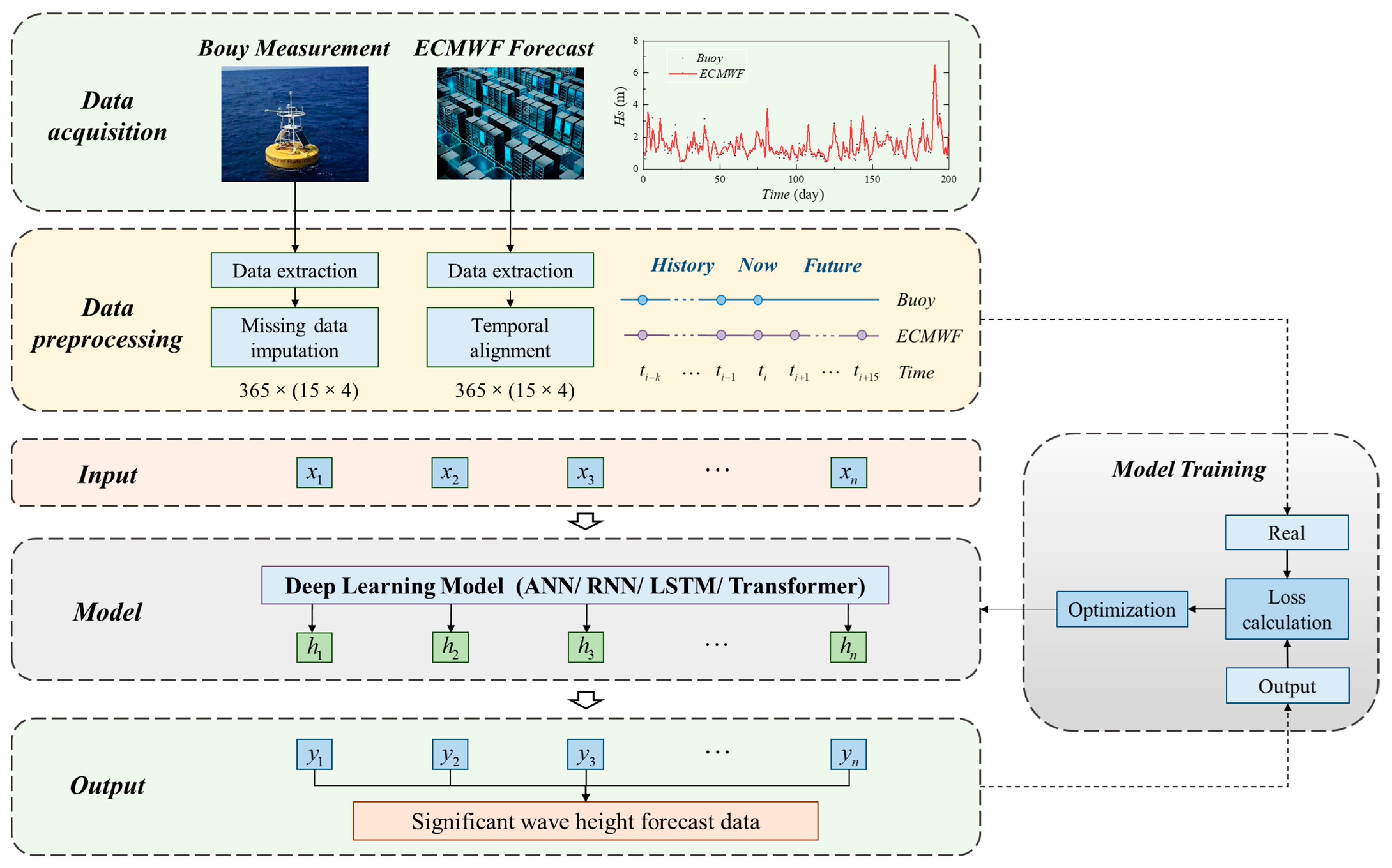
This study uses deep learning methods to construct the Wave Forecast Artificial Intelligence (WF-AI) model. Based on buoy measurements and ECMWF forecast results, the model achieves predictions of Hs for the next 1 to 15 days. The specific structure of the model is illustrated in Figure 5.

Figure 5. The schematic diagram of the WF-AI model structure.

The first step involves data acquisition and pre-processing. The model data are obtained from the NDBC and ECMWF databases. The NDBC provides buoy measurement data. However, due to the influence of data collection equipment and extreme weather conditions, specific data gaps are present at various buoy locations. The observed data need to be processed to extract significant wave height results. Additionally, a linear interpolation method is applied to fill in missing wave height data along the time dimension. Regarding the ECMWF forecast data, varying time resolutions exist depending on the forecast time. Both datasets are processed separately and standardised to a temporal resolution of 6 h. After processing, the dimension of the univariate data is 365 × 60. Here, 60 represents the wave data updated every six hours over the next 15 days. In the three buoys, buoy 41040 is used for model accuracy analysis, while buoys 44008 and 41048 are used for model adaptability analysis. For each buoy location, 80% of the dataset is used for model training, with the remaining 20% reserved for model testing.

Secondly, the model’s inputs and outputs are detailed. The constructed model incorporates deep learning modules, which use the ANN, RNN, LSTM, and Transformer methods for wave modelling. The proposed model is used to forecast wave conditions by training and validating each model at time frames of 1, 3, 6, 10, 12, and 15 days, respectively. The forecasting performance of different deep learning approaches is compared. The ECMWF dataset includes wave data for the present time and the following 15 days, while buoy data consists of current and historical wave records. For model outputs, error calculations are conducted for forecasts generated every 6 h (i.e., four times daily) at specific forecast durations, which serve as indicators of daily wave forecasting accuracy.

Furthermore, the optimisation of model performance is addressed. The differences in forecasting outcomes under various input strategies are examined for different forecast durations. Taking the 1-day forecast as an example, the model input variables comprise the 1-day forecast for Hs from ECMWF (EC_t1), the 0-day forecast for Hs from ECMWF (EC_t0), and the buoy-measured Hs (Buoy_t0). Through combinations, a total of four input schemes are ultimately established, as presented in Table 2. Similarly, for forecasts ranging from 3 to 15 days, a comparable approach is employed to contrast the forecasting results across different input time series. When the forecast period extends to 15 days, the inputs for comparison include [EC_t0, EC_t1, …, EC_t15], [EC_t0, EC_t1, …, EC_t15, Buoy_t−15, …, Buoy_t−1, Buoy_t0], and [EC_t15, Buoy_t0], among others. The model ultimately achieves wave forecasting for the following 15 days.

Table 2. Model input design of the WF-AI model for Forecast-1d.

Model Design		Variable
Input	1	ECt1
	2	ECt1, ECt0
	3	ECt1, Buoyt0
	4	ECt1, ECt0, Buoyt0
Output		Buoyt1

3.2. Deep Learning Models

3.2.1. Artificial Neural Networks

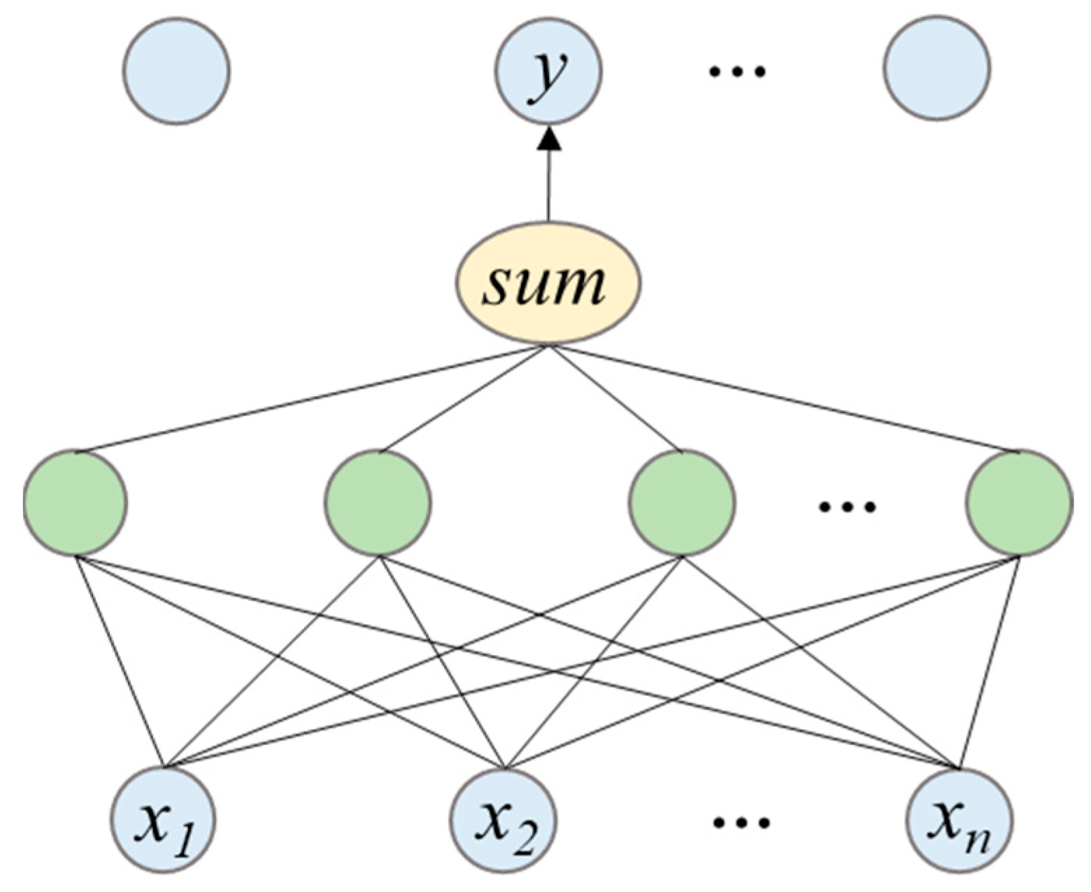
Artificial Neural Networks (ANNs) are a class of computational models inspired by biological neural networks designed to simulate the structure and information transmission of neurons in the human brain [38]. The basic architecture consists of multiple nodes (neurons) and layers (input layer, hidden layers, output layer), with the connections between nodes referred to as “weights.” ANNs learn and represent nonlinear relationships in data by adjusting these weights. Currently, ANNs are primarily used for various tasks, including classification, regression, and pattern recognition, as the foundational framework for deep learning models. The structure of an ANN is illustrated in Figure 6.

Figure 6. Structure diagram of ANN.

The output of an ANN can be represented as

$$y = F({\displaystyle \sum _{k=1}^{n}W{x}_k}+b)$$

(1)

where x and y represent the model’s input and output, respectively; W and b represent the model’s weights and bias coefficients. The model can incorporate multiple inputs x₁, x₂, …, x_n, continuously extracting data features through a multilayer network while introducing nonlinearity via activation functions, ultimately producing the model output y.

3.2.2. Recurrent Neural Networks

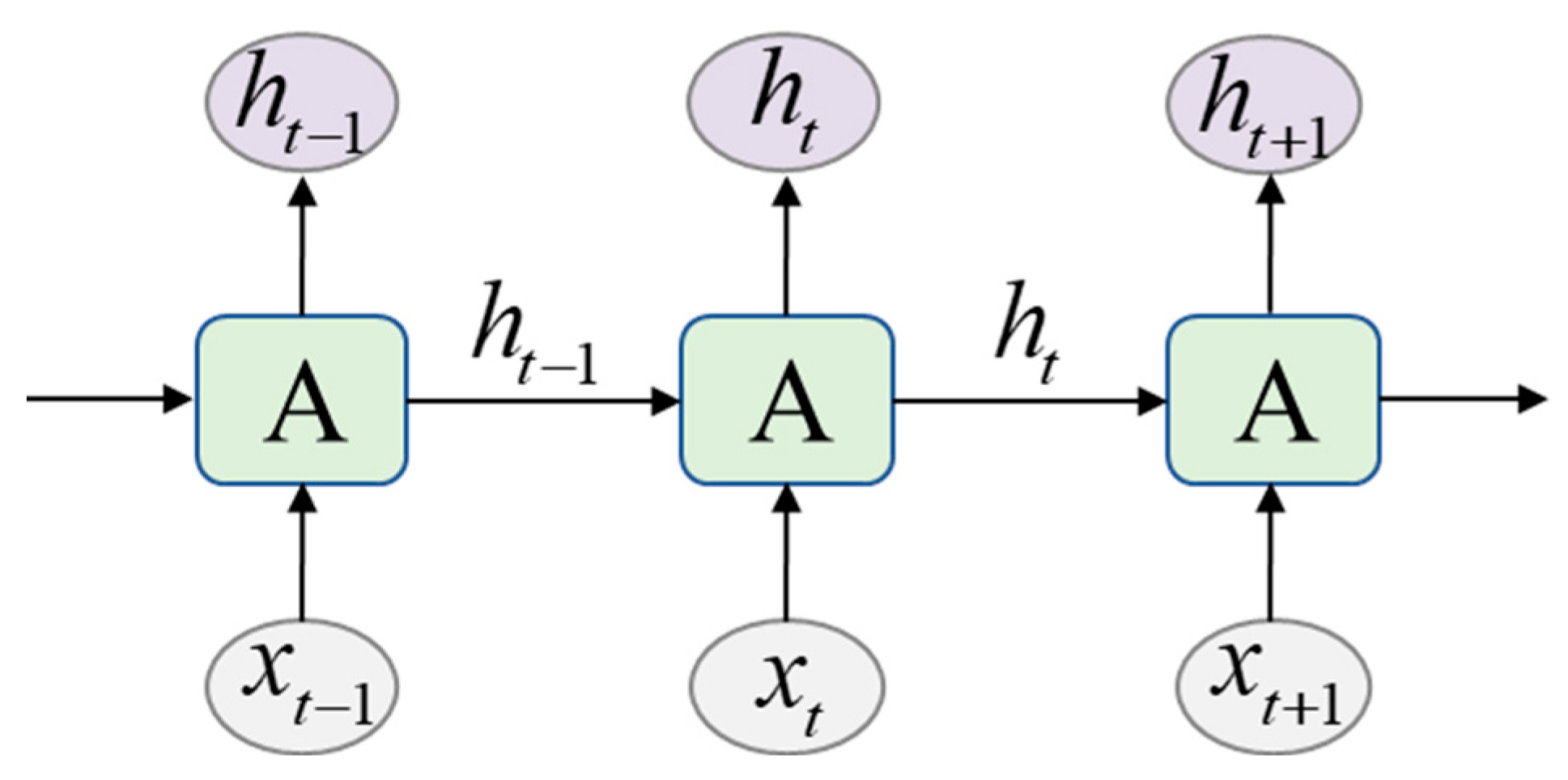
Recurrent Neural Networks (RNNs), represent a neural network model primarily designed for processing sequential data [39]. RNNs use a cyclic structure that incorporates the output from the previous time step as input for the current time step, thereby preserving the continuity of information within the time series. This architecture effectively addresses the issue of context information lacking in traditional neural networks when dealing with ordered data such as time series and natural language. The specific structure is illustrated in Figure 7.

Figure 7. Structure diagram of RNN.

The output of an RNN can be represented as

$$h_t= G(W{x}_t+U{h}_{t-1})$$

(2)

$$y_t=F\left(h_t\right)$$

(3)

where x_t denotes the model input at time t; W and U represent the weight coefficients from the input layer to the hidden layer and from the hidden layer to the output layer, respectively; and h_t indicates the state of the hidden layer. As illustrated in the figure and calculation method, the current hidden layer state in the model depends not only on the current input but also on the state of the hidden layer at the previous time step.

3.2.3. Long Short-Term Memory

Long Short-Term Memory (LSTM) is a specific form of RNN that effectively addresses the problem of long-term dependencies while mitigating the issues of gradient vanishing and gradient explosion commonly encountered in traditional RNN models [40]. The LSTM model comprises a forget gate, an input gate, an output gate, and a memory cell. It employs three gating units to control the flow of information, establishing delays among input, feedback, and output while continuously updating the cell state through the memory cell. The specific structure is illustrated in Figure 8.

Figure 8. Structure diagram of LSTM.

The output of a LSTM can be represented as

$$f_t=\sigma \left(W_f\left[h_{t-1},x_t\right]+b_f\right)$$

(4)

$$i_t=\sigma (W_i[h_{t-1},x_t]+b_i)$$

(5)

$$o_t=\sigma \left(W_o\left[h_{t-1},x_t\right]+b_o\right)$$

(6)

$${\widehat{C}}_t=\tanh (W_c[h_{t-1},x_t]+b_c)$$

(7)

$$C_t=f_t\ast C_{t-1}+i_t\ast {\widehat{C}}_t$$

(8)

where f, i, and o denote the forget gate, input gate, and output gate, respectively, while C represents the information storage state of the neuron, and t indicates the current neuron.

$$h_t=o_t\ast \tanh \left(C_t\right)$$

(9)

$$y_t=F\left(h_t\right)$$

(10)

In Equations (9) and (10), W and b represent the weight coefficient and bias in the model, respectively. h and y denote the hidden layer and the model output, respectively.

3.2.4. Transformer

The Transformer model, proposed by Vaswani et al. [41], is designed for addressing translation tasks. This model effectively overcomes the efficiency and parallelisation issues encountered by traditional recurrent neural networks (RNN and LSTM) when processing long sequences. By discarding the recursive structure, the Transformer employs a self-attention mechanism, allowing for better capture of dependencies among elements within a sequence. The model uses the self-attention mechanism to focus on the parts deemed necessary.

During the propagation process of the self-attention layer, the input x_t is transformed through weight coefficients [W_q,W_k,W_v] to generate corresponding representations [q_t,k_t,v_t]. The vectors q_t and k_t undergo a SoftMax transformation and are summed with v_t to produce the output result h_t at that moment. The specific structure is illustrated in Figure 9.

Figure 9. Diagram of the self-attention structure in the Transformer model.

The output of a Transformer can be represented as

$$q_t=x_t{W}_q$$

(11)

$$k_t=x_t{W}_k$$

(12)

$$v_t=x_t{W}_v$$

(13)

$$h_t={\displaystyle \sum soft\max (q_t·k_t/\sqrt{d_k})·v_t}$$

(14)

where t denotes the current time, x represents the input vector, and h indicates the output after self-attention. q, k, and v correspond to the three attributes of the input: query, key, and value, respectively. W_q, W_k, and W_v are the associated weight coefficients. d_k represents the square root of the dimension of k.

Additionally, to comprehensively extract features from the input data, the Transformer model employs a multi-head self-attention mechanism consisting of multiple self-attention layers. Multiple sets of weight coefficients are initialised simultaneously for the input vectors. Finally, the results from these multiple sets are concatenated and combined with the weight coefficients W^o to produce the final output. The specific structure is illustrated in Figure 10.

$$h_t=concat(h_t^1,h_t^2,\cdots ,h_t^n)W^o$$

(15)

Figure 10. Schematic diagram of multi-head self-attention.

At time t, in Equation (15), n represents the number of attention heads, $h_t^1,h_t^2,···,h_t^n$ represent the computation result of different attention heads, and W^o denotes the trainable weight coefficient.

4. Results and Discussion

This section investigates the WF-AI model’s forecasting accuracy for Hs over the next 15 days in the United States East Coast waters. The differences in forecasting results are compared across various deep learning methods, including ANN, RNN, LSTM, and Transformer. The model’s adaptability to different locations and water depths within the study area is also analysed.

This study employs the Mean Absolute Error (MAE), Root Mean Square Error (RMSE), Mean Absolute Percentage Error (MAPE), and Pearson’s Correlation Coefficient (r) as the accuracy evaluation metrics.

$$\mathrm{MAE}={\displaystyle \frac{{\displaystyle \sum _{i=1}^n\left|H{s}_{tru\_i}-H{s}_{pre\_i}\right|}}{n}}$$

(16)

$$\mathrm{RMSE}=\sqrt{{\displaystyle \frac{{\displaystyle \sum _{i=1}^n{\left(H{s}_{tru\_i}-H{s}_{pre\_i}\right)}^2}}{n}}}$$

(17)

$$\mathrm{MAPE}={\displaystyle \frac{1}{n}}{\displaystyle \sum _{i=1}^n\left|\frac{H{s}_{tru\_i}-H{s}_{pre\_i}}{H{s}_{pre\_i}}\right|}$$

(18)

$$\mathrm{r}={\displaystyle \frac{{\displaystyle \sum _{i=1}^n\left(H{s}_{tru\_i}-\frac{1}{n}{\displaystyle \sum _{i=1}^{n}H{s}_{tru\_i}}\right)\left(H{s}_{pre\_i}-\frac{1}{n}{\displaystyle \sum _{i=1}^{n}H{s}_{pre\_i}}\right)}}{\sqrt{{\displaystyle \sum _{i=1}^n{\left(H{s}_{tru\_i}-\frac{1}{n}{\displaystyle \sum _{i=1}^{n}H{s}_{tru\_i}}\right)}^2}{\displaystyle \sum _{i=1}^n{\left(H{s}_{pre\_i}-\frac{1}{n}{\displaystyle \sum _{i=1}^{n}H{s}_{pre\_i}}\right)}^2}}}}$$

(19)

In Equations (16)–(19), n represents the sample size, and Hs_{tru_i} and Hs_{pre_i} denote the buoy measurement results and forecast results at time i, respectively.

4.1. Accuracy Analysis

The WF-AI model is used to forecast Hs over the following 15 days in the eastern coastal waters of the United States. In addition, the forecasting performance of various deep learning methods, including ANN, RNN, LSTM, and Transformer, is compared.

For the current model, analysis shows that for forecasts of 1, 3, 6, and 10 days, the model achieves the highest accuracy only when the ECMWF data corresponding to the forecast time is used as input. For forecasts extending to 12 and 15 days, the inclusion of buoy data for the current time significantly enhances accuracy. Finally, the optimal model inputs for different forecast periods are summarised in Table 3.

Table 3. Optimal input for the WF-AI model.

No.	Forecast Time (Day)	Time Series	Input Variable
1	1	ECt1	Hs
2	3	ECt3	Hs
3	6	ECt6	Hs
4	10	ECt10	Hs
5	12	ECt12, Buoyt0	Hs, Buoy
6	15	ECt15, Buoyt0	Hs, Buoy

The Hs forecast results of the WF-AI model for periods of 1, 3, 6, 10, 12, and 15 days at Buoy 41040 are analysed. The ECMWF dataset is compared [42,43]. The specific error calculations are presented in Table 4 and Figure 11.

Table 4. Forecast errors of Hs for the next 15 days.

Forecast Time (Day)	Models	MAE (m)	RMSE (m)	MAPE (%)	r
1	ECMWF	0.13	0.16	5.84	0.96
	ANN	0.11	0.15	4.88	0.95
	RNN	0.13	0.16	5.59	0.94
	LSTM	0.13	0.17	5.89	0.93
	Transformer	0.12	0.15	5.34	0.95
3	ECMWF	0.15	0.18	6.72	0.94
	ANN	0.14	0.17	6.04	0.93
	RNN	0.14	0.18	6.17	0.93
	LSTM	0.15	0.19	6.52	0.92
	Transformer	0.14	0.18	6.30	0.93
6	ECMWF	0.18	0.22	8.10	0.89
	ANN	0.17	0.22	7.45	0.89
	RNN	0.17	0.22	7.74	0.88
	LSTM	0.17	0.22	7.79	0.88
	Transformer	0.17	0.22	7.67	0.89
10	ECMWF	0.29	0.36	13.08	0.71
	ANN	0.29	0.35	12.37	0.71
	RNN	0.29	0.35	12.29	0.71
	LSTM	0.28	0.34	12.09	0.72
	Transformer	0.26	0.33	11.88	0.72
12	ECMWF	0.38	0.47	17.13	0.49
	ANN	0.33	0.42	15.00	0.50
	RNN	0.34	0.42	14.79	0.49
	LSTM	0.34	0.42	14.75	0.50
	Transformer	0.33	0.41	14.77	0.50
15	ECMWF	0.49	0.61	22.52	0.33
	ANN	0.40	0.50	18.74	0.34
	RNN	0.36	0.44	16.32	0.34
	LSTM	0.36	0.44	16.54	0.35
	Transformer	0.37	0.45	16.43	0.34

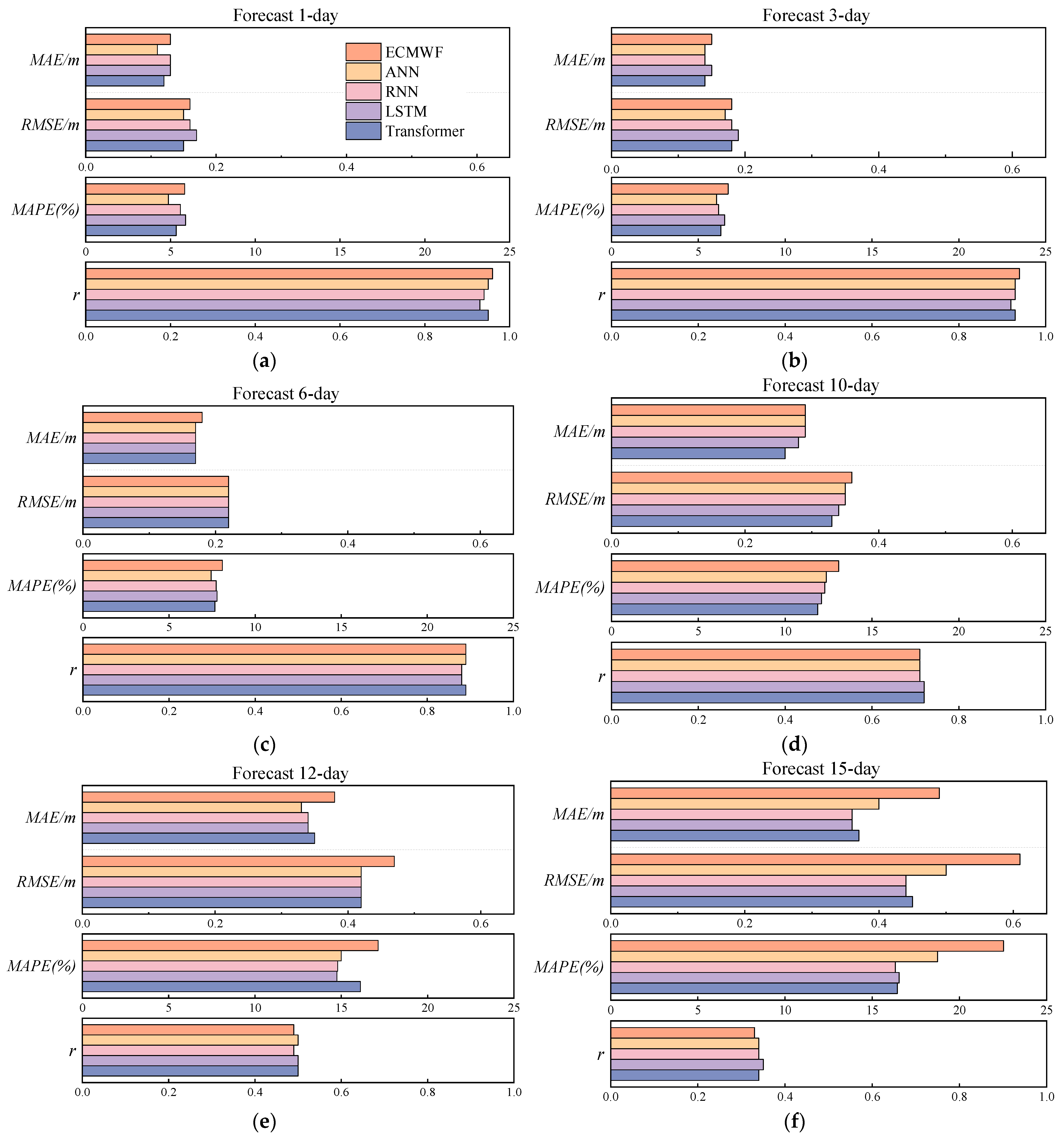
Figure 11. Forecast errors for the next 15 days. (a–f) represent forecast errors for 1, 3, 6, 10, 12, and 15 days, respectively.

In Figure 11a–f illustrate the variation of model errors at different forecast lead times. For each forecast duration, the MAE, RMSE, MAPE, and r are displayed on the same scale to facilitate the comparison of error variations over time. The comparison indicates a gradual decline in forecasting accuracy for both the ECMWF and WF-AI models as the forecast lead time increases.

For a 1-day forecast, the model demonstrates high accuracy in wave prediction, with MAE/RMSE/MAPE values below 0.13 m/0.16 m/5.89%, respectively, and r exceeding 0.93. When the forecast lead time reaches 6 days, the MAE/RMSE/MAPE is less than 0.18 m/0.22 m/8.10%, respectively, while r exceeds 0.88. At this stage, the forecasting errors remain within 10%, indicating a high accuracy in predicting Hs.

A decrease in model accuracy occurs when the forecast lead time reaches 10 days. The MAPE of the ECMWF model is 13.08%. The accuracy of the WF-AI model is slightly better than that of the ECMWF, with minimum values of MAE/RMSE/MAPE reaching 0.26 m/0.33 m/11.88%, respectively, and an r value of 0.72.

A noticeable decline in forecasting accuracy occurs when the forecast lead time reaches 12 days. The MAPE for the ECMWF and WF-AI models is 17.13% and 14.75%, respectively. At a 15-day forecast, the ECMWF model exhibits poor accuracy for Hs, with MAE/RMSE/MAPE/r values of 0.49 m/0.61 m/22.52%/0.33.

In contrast, the WF-AI model shows improved accuracy compared to ECMWF, with MAE/RMSE/MAPE/r values of 0.36 m/0.44 m/16.32%/0.35. It can be observed that as the forecasting time increases, the prediction accuracy of both the ECMWF and WF-AI models declines.

Both models exhibit relatively good accuracy for lead times of 1–6 days. In the 10–15-day forecasts, the accuracy of both models decreases; however, the WF-AI model demonstrates better performance than the ECMWF.

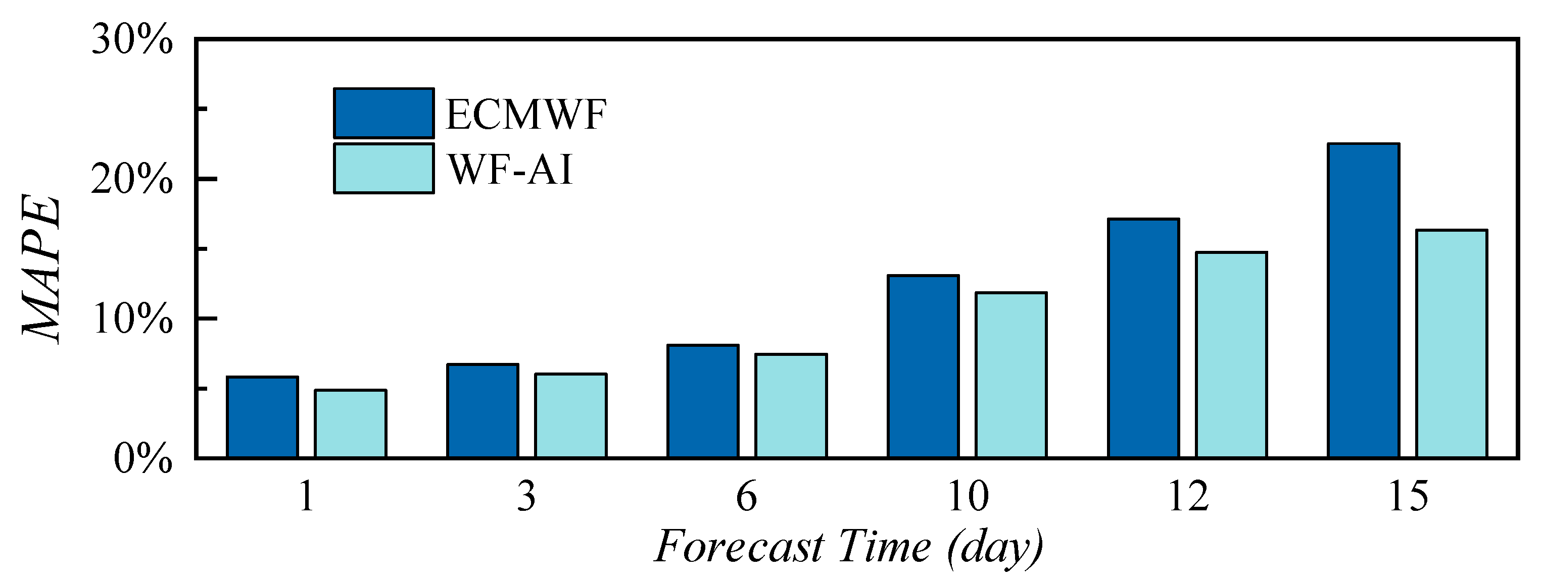
Furthermore, a comparison of the wave forecasting results between the WF-AI model and ECMWF is presented in Figure 12. The forecasting error analysis indicates that both models exhibit high forecasting accuracy for lead times of 1–6 days, with the WF-AI model demonstrating slightly higher accuracy than the ECMWF. In this period, the MAPE for both models remains below 10%.

Figure 12. Comparison of wave forecasting errors between the WF-AI model and ECMWF.

The differences in forecast accuracy between the two models become gradually apparent when the forecast time exceeds 10 days. The forecast errors for both models increase with the length of the forecast period. However, the WF-AI model accurately predicts Hs more accurately than ECMWF. When the forecast lead time reaches 15 days, the WF-AI model achieves a MAPE of 16.32%, better than the ECMWF’s 22.52%.

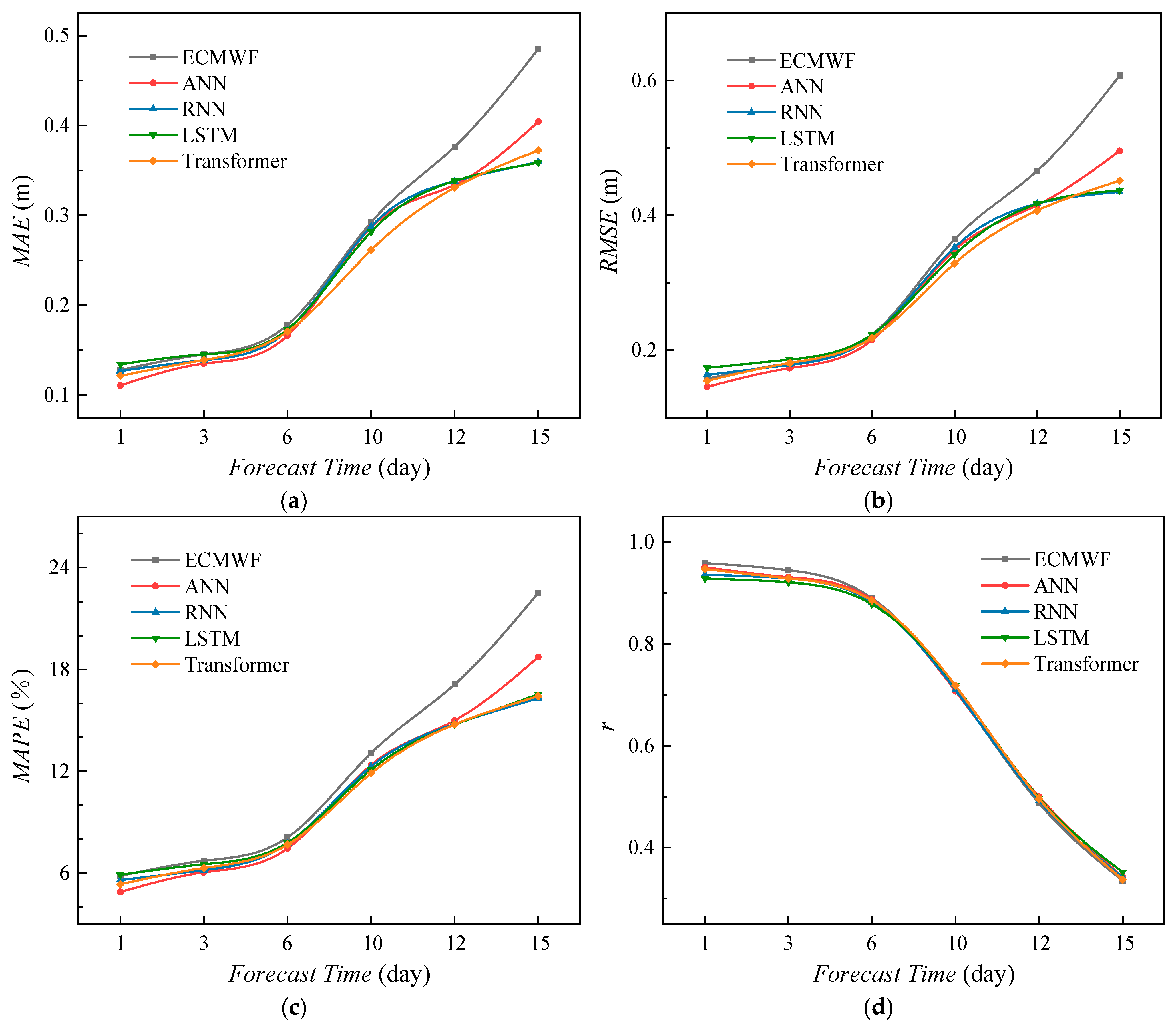
Additionally, the differences in wave forecasting results of the WF-AI model under various deep learning methods are presented, as shown in Figure 13. The comparison reveals that the RNN, LSTM, and Transformer methods achieve comparable accuracy in wave forecasting, as measured by MAE, RMSE, and MAPE evaluation metrics.

Figure 13. Comparison of wave forecasting errors under different methods. (a–d) represent MAE, RMSE, MAPE, and r, respectively.

The ANN method demonstrates slightly better forecasting accuracy in the early stages than other deep learning approaches. It was noted that the ANN model ignores the temporal correlations among data, which influences the long-term wave forecasts. It can be seen that the overall accuracy of the ANN method remains better than the ECMWF method, and the r of all models gradually decreases with increasing forecast time, indicating a weakening correlation between wave forecast results and the observed buoy values over time.

Overall, the WF-AI model demonstrates better accuracy in predicting Hs than the ECMWF forecast, particularly in medium- to long-term forecasts, with lower errors and suggesting improved stability and accuracy in Hs prediction tasks.

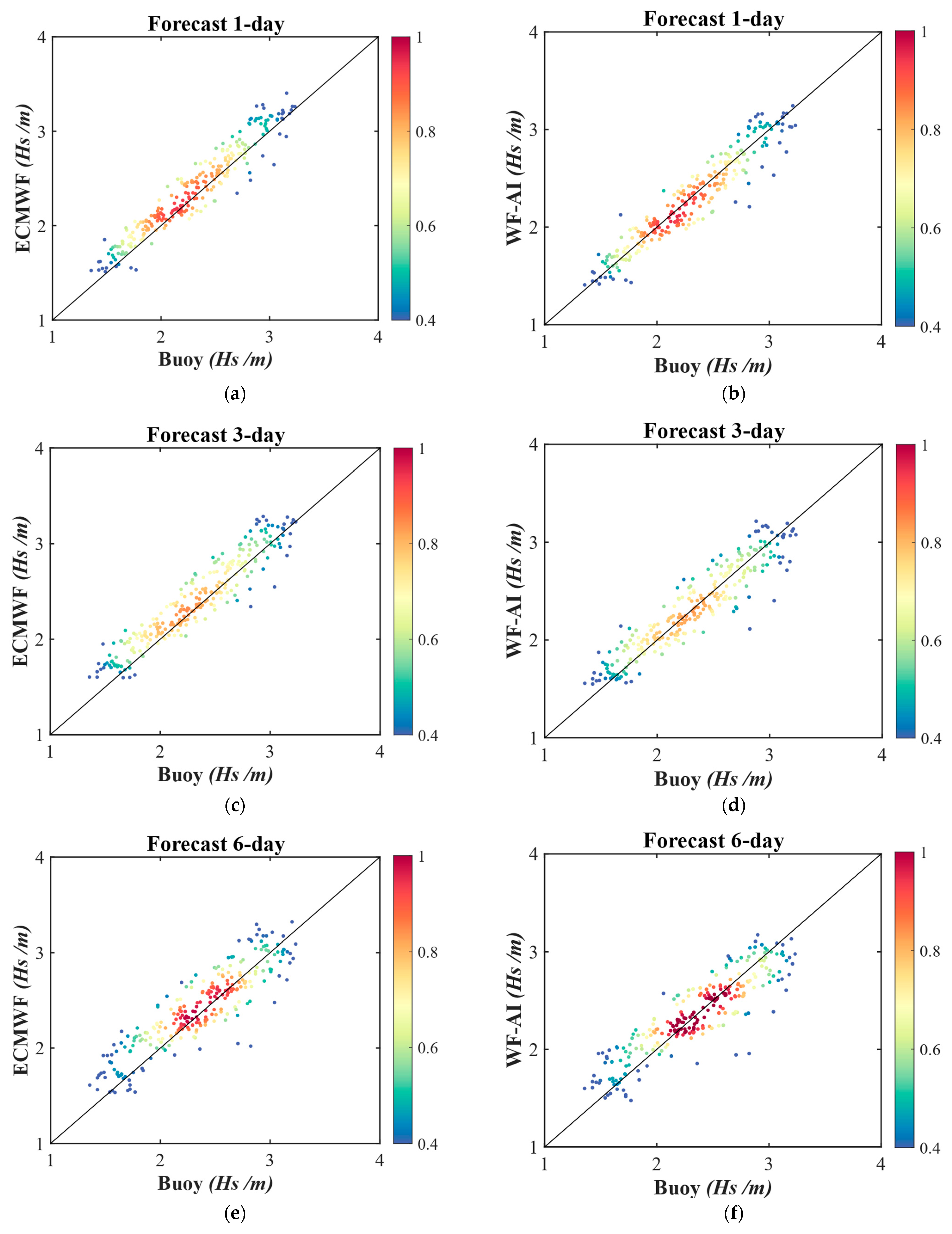
Further analysis of the correlation between the WF-AI model and ECMWF wave forecasting results, using buoy measurements, is conducted, as illustrated in Figure 14. The comparison indicates that the correlation between the wave prediction results and the true values gradually weakens as the forecasting time increases. However, the correlation for the WF-AI model predictions in the right column remains superior to the ECMWF forecasting results on the left, particularly evident in the 10–15 day forecast range.

Figure 14. Comparison of wave forecasting correlation between ECMWF and the WF-AI models. (The left columns (a,c,e,g,i,k) represent ECMWF wave forecasting results, while the right columns (b,d,f,h,j,l) represent the WF-AI model wave forecasting results. From top to bottom, the rows correspond to wave forecasts for 1, 3, 6, 10, 12, and 15 days.)

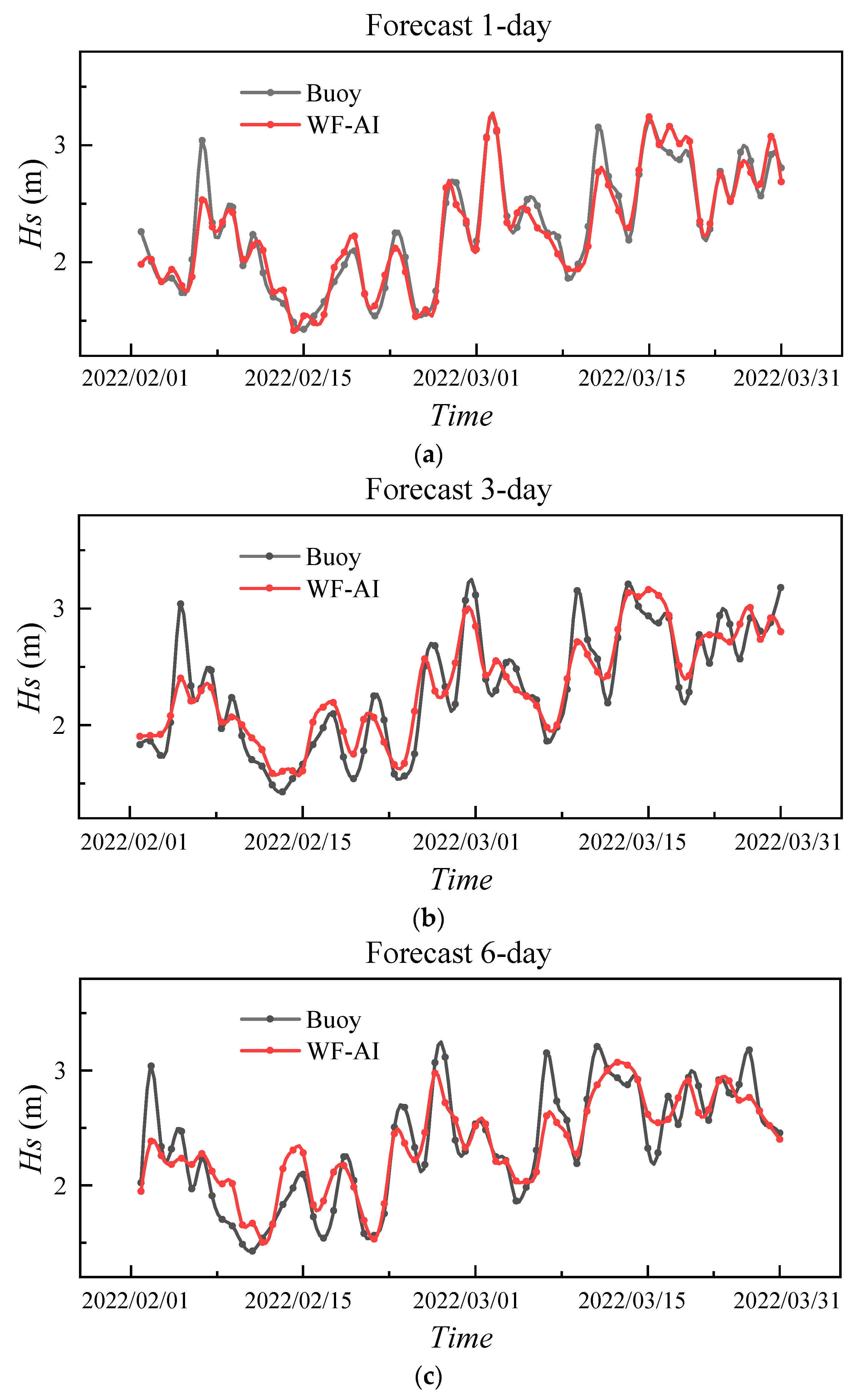
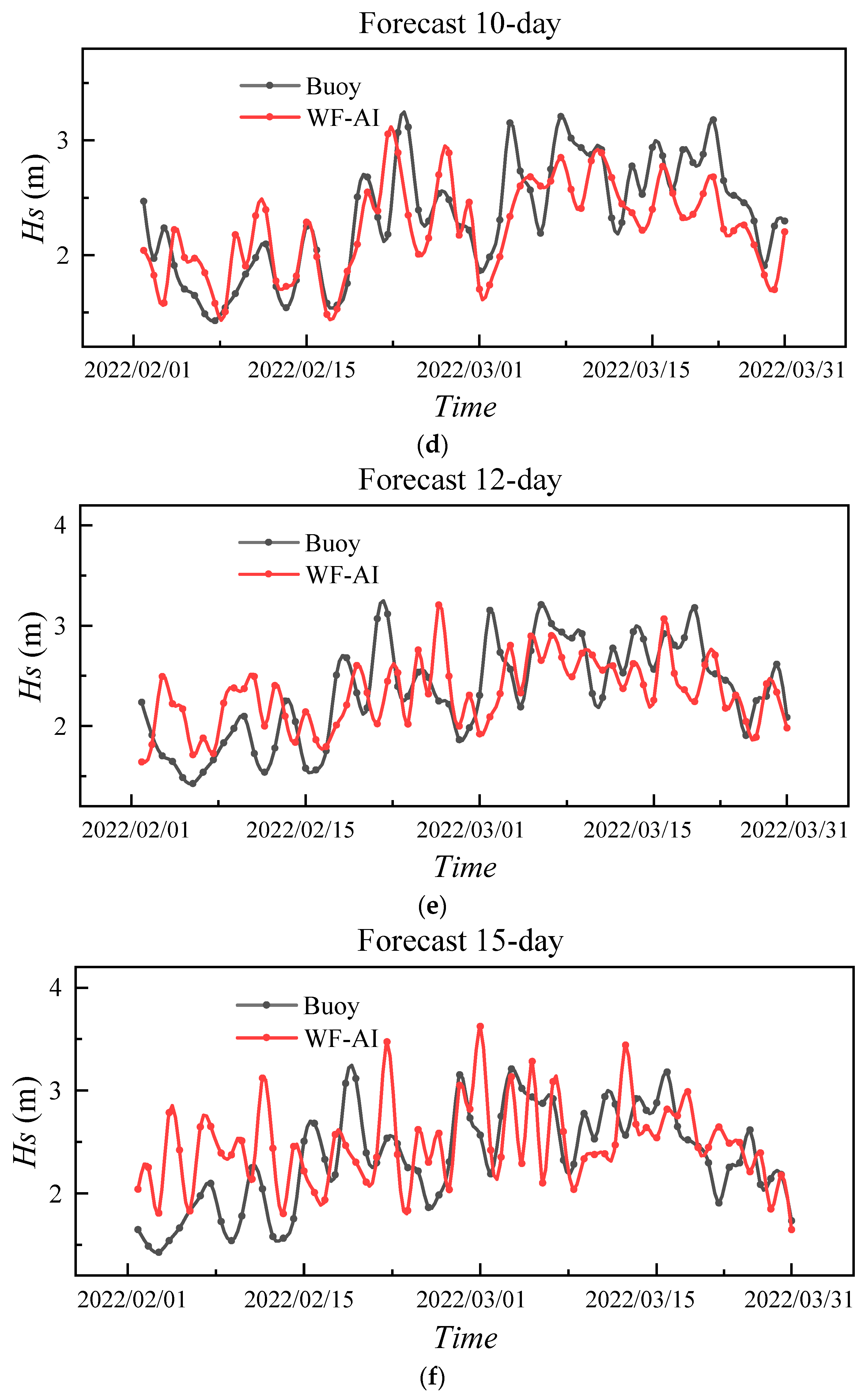
The Hs forecasting results of the WF-AI model are compared with buoy data in Figure 15 for different forecasting durations. The variations in model-predicted Hs for 1, 3, 6, 10, 12, and 15 days are illustrated in Figure 15.

Figure 15. Wave forecasting results of the WF-AI model for the next 1, 3, 6, 10, 12, and 15 days. (a) Forecast 1-day; (b) Forecast 3-day; (c) Forecast 6-day; (d) Forecast 10-day; (e) Forecast 12-day; (f) Forecast 15-day.

It can be observed that the WF-AI model effectively forecasts wave conditions for the next 15 days. The accuracy is notably high for the 1–6 day forecasts, with the model predictions aligning closely with buoy measurements. The forecast accuracy for the 10–15 day range is slightly lower than that of the earlier period, with MAPE values of 11.88%, 14.75%, and 16.32% for the 10-, 12-, and 15-day forecasts, respectively. However, these values are more accurate compared to ECMWF predictions.

Finally, the forecasting performance of the model under extreme sea states is analysed. The prediction skill of ECMWF and the WF-AI model for sea states 6 and 7 over the 1–15 day forecast period is presented in Table 5. In addition, the results are evaluated using the mean, standard deviation, and 95% confidence intervals of these differences. The specific calculation methods are as follows:

$${\delta }_{Hs}=|H{s}_{cal}-H{s}_{buoy}|$$

(20)

$$\overline{X}={\displaystyle \frac{1}{n}}{\displaystyle \sum _{i=1}^n{X}_i}$$

(21)

$$s=\sqrt{{\displaystyle \frac{1}{n-1}}{{\displaystyle \sum _{i=1}^n\left(X_i-\overline{X}\right)}}^2}$$

(22)

$$CI=\left(\overline{X}-1.96·{\displaystyle \frac{s}{\sqrt{n}}},\overline{X}+1.96·{\displaystyle \frac{s}{\sqrt{n}}}\right)$$

(23)

Table 5. Forecast errors of Hs under extreme sea states.

Forecast Time (Day)	Models	Sea State 6				Sea State 7
		MAE (m)	RMSE (m)	MAPE (%)	r	MAE (m)	RMSE (m)	MAPE (%)	r
1	ECMWF	0.13	0.16	5.10	0.89	0.10	0.14	3.34%	0.44
	WF-AI	0.12	0.15	4.93	0.88	0.11	0.18	3.59%	0.33
3	ECMWF	0.14	0.17	5.53	0.87	0.17	0.20	10.35%	0.76
	WF-AI	0.13	0.17	5.39	0.84	0.13	0.16	7.68%	0.73
6	ECMWF	0.16	0.21	6.41	0.76	0.23	0.26	13.32%	0.68
	WF-AI	0.14	0.19	5.74	0.75	0.20	0.23	11.79%	0.66
10	ECMWF	0.30	0.37	12.31	0.50	0.28	0.35	16.33%	0.39
	WF-AI	0.29	0.34	11.59	0.50	0.23	0.28	13.42%	0.43
12	ECMWF	0.34	0.42	14.03	0.31	0.43	0.53	25.65%	0.16
	WF-AI	0.29	0.36	11.52	0.33	0.38	0.46	23.11%	0.17
15	ECMWF	0.42	0.53	17.23	0.32	0.67	0.79	39.56%	0.14
	WF-AI	0.32	0.40	13.16	0.32	0.58	0.67	34.60%	0.14

In Equations (20)–(23), δ_Hs represents the absolute difference between the model calculations and the buoy observations. $\overline{X}$ represents the sample mean, s represents the sample standard deviation, and CI represents the 95% confidence interval. X_i represents the sample data, and n represents the sample size.

A comparison reveals that under extreme sea conditions, the model outperforms the ECMWF in terms of accuracy. For forecasts of the next 10, 12, and 15 days, the WF-AI model achieves a MAPE not exceeding 13.16% for sea state 6. Specifically, the ECMWF model shows δ_Hs = 0.30 ± 0.22 (±s), CI = (0.271, 0.326); δ_Hs = 0.34 ± 0.25, CI = (0.311, 0.373); and δ_Hs = 0.42 ± 0.33, CI = (0.380, 0.462) for the 10-, 12-, and 15-day forecasts, respectively. In comparison, the WF-AI model demonstrates δ_Hs = 0.29 ± 0.19, CI = (0.261, 0.310); δ_Hs = 0.29 ± 0.21, CI = (0.260, 0.313); and δ_Hs = 0.32 ± 0.23, CI = (0.300, 0.353) for the same forecast periods, respectively. However, for sea state 7, the model’s forecasting accuracy is relatively poorer. Specifically, the ECMWF model shows δ_Hs = 0.29 ± 0.26, CI = (0.253, 0.319); δ_Hs = 0.50 ± 0.34, CI = (0.458, 0.543); and δ_Hs = 0.49 ± 0.33, CI = (0.451, 0.534) for the 10-, 12-, and 15-day forecasts, respectively. In comparison, the WF-AI model shows δ_Hs = 0.49 ± 0.24, CI = (0.454, 0.515); δ_Hs = 0.58 ± 0.32, CI = (0.535, 0.616); and δ_Hs = 0.55 ± 0.33, CI = (0.510, 0.592) for the same forecast periods, respectively. This discrepancy is primarily due to the significantly reduced number of sea state 7 occurrences, leading to fewer training samples. Therefore, there is still room for improvement in the model’s forecasting accuracy for extreme weather conditions.

The WF-AI model effectively enhances the forecasting accuracy of waves over long periods, showing improvements compared to ECMWF. Nevertheless, the current model still faces certain limitations in its application. While the model improves the accuracy of existing wave forecasting methods for long periods, discrepancies remain when compared to actual wave values. As illustrated above in Figure 15f, there is still potential for improvement, particularly in forecasting extreme wave conditions. Additionally, the WF-AI model relies on existing wave forecast data and observational results for forecasting. As a result, the forecast accuracy is influenced by outcomes such as those from ECMWF IFS. Additionally, when observational data is missing, it can also affect the model’s forecasting performance to some extent.

4.2. Adaptability Analysis

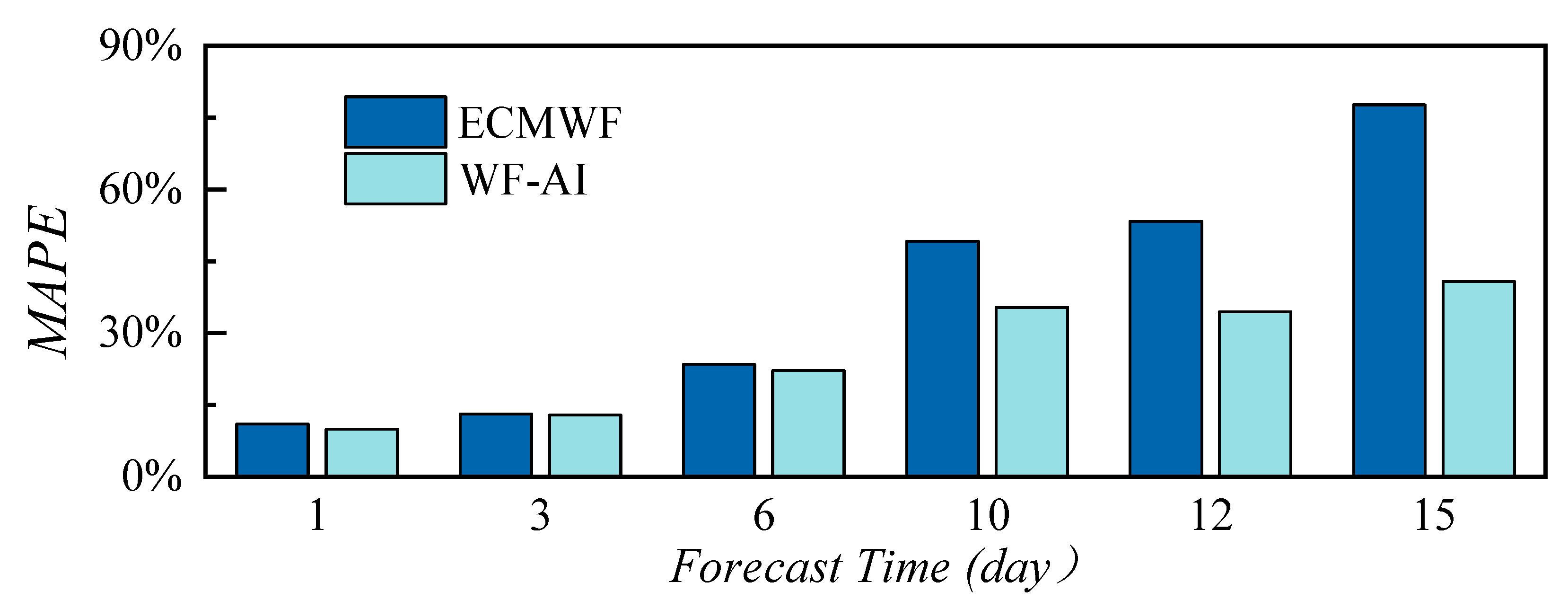
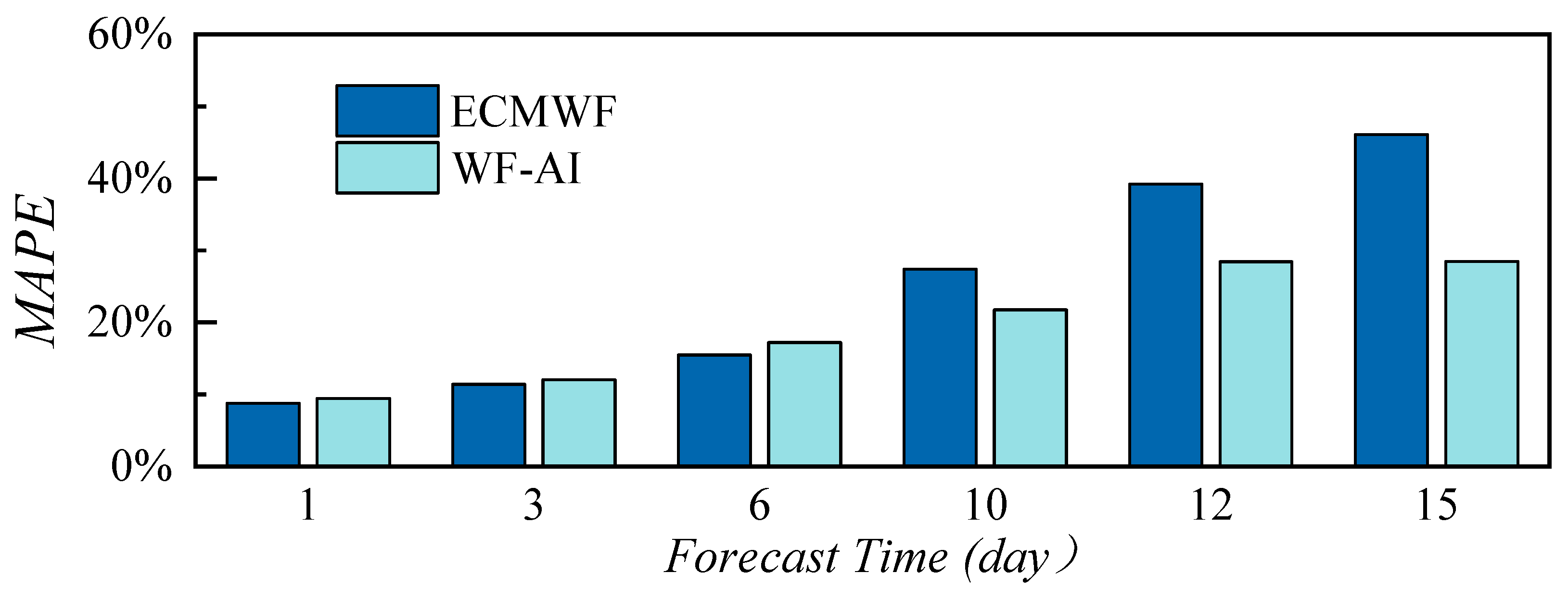
Further analysis is conducted on the adaptability of the WF-AI model. For the western Atlantic Ocean, Buoy 44008 and 41048 are selected to test the model’s performance. An analysis of the Hs predictions from the WF-AI model for the next 1 to 15 days is conducted and compared with the ECMWF results. Due to the varying locations of the buoys and the influence of factors such as water depth, the accuracy of the ECMWF dataset also exhibits certain differences. The specific error calculation results are presented in Table 6. Further graphical analysis of the error trends at the two buoy locations is presented in Figure 16 and Figure 17.

Table 6. Wave forecasting errors for the next 15 days at other locations.

Forecast Time (Day)	Methods	Buoy 44008#		Buoy 41048#
		MAE (m)	MAPE (%)	MAE (m)	MAPE (%)
1	ECMWF	0.23	10.96	0.22	8.74
	WF-AI	0.23	9.96	0.24	9.42
3	ECMWF	0.28	13.14	0.27	11.40
	WF-AI	0.29	12.88	0.29	12.01
6	ECMWF	0.47	23.45	0.36	15.46
	WF-AI	0.50	22.14	0.42	17.25
10	ECMWF	0.86	49.16	0.53	27.38
	WF-AI	0.74	35.37	0.49	21.76
12	ECMWF	0.91	53.30	0.76	39.20
	WF-AI	0.72	34.50	0.64	28.41
15	ECMWF	1.25	77.67	0.75	46.09
	WF-AI	0.91	40.78	0.67	28.43

Figure 16. Comparison of the WF-AI model and ECMWF wave forecasting errors at Buoy 44008.

Figure 17. Comparison of the WF-AI model and ECMWF wave forecasting errors at Buoy 41048.

The comparison reveals that the proposed WF-AI model provides higher accuracy in forecasting Hs for the following 15 days than ECMWF. Notably, for more extended forecasting periods (10–15 days), the accuracy of the WF-AI model shows a significant improvement over ECMWF forecasts.

Additionally, Figure 18 presents the wave forecasting results of the WF-AI model under various deep learning methods. The forecasting accuracy across different methods is similar, with all methods achieving higher accuracy than ECMWF in long-term wave forecasting tasks. It can be further indicated that the WF-AI model effectively enhances the forecasting accuracy of wave heights over the next 15 days, particularly for long-term predictions of Hs, surpassing the accuracy of ECMWF.

Figure 18. Comparison of wave forecast errors at Buoy 44008 and 41048 using different methods. (a) Buoy 44008; (b) Buoy 41048.

5. Conclusions

This study uses deep learning techniques to propose a wave forecasting model (WF-AI). Using buoy measurements and wave data provided by ECMWF, long-term forecasting of significant wave height (particularly for the next 10–15 days) can be achieved. Analysis of the results leads to the following conclusions: (1) The WF-AI model significantly enhances wave forecasting accuracy compared to existing methods, particularly for long-term wave predictions. At Buoy 41040, the MAPE for forecasting Hs over horizons of 1, 3, 6, 10, 12, and 15 days is 4.89%, 6.04%, 7.45%, 11.88%, 14.75%, and 16.32%, respectively. Notably, for the 10/12/15-day forecasts, the MAPE is lower than that of the ECMWF predictions, which are 13.08%, 17.13%, and 22.52%. This indicates that the WF-AI model outperforms ECMWF in long-term wave forecasting.

(2) The forecasting accuracy of different deep learning methods is comparable for long-term wave forecasting tasks. Specifically, the RNN, LSTM, and Transformer methods account for the temporal correlation within the data. In the context of the wave forecasting task addressed in this study, the accuracies of these three methods are similar and exhibit the same trend. In comparison, ANN demonstrates higher accuracy during the initial forecasting period; however, its accuracy for long-term predictions, particularly beyond 10 days, is slightly lower than that of the other methods.

(3) The WF-AI model demonstrates good adaptability to the sea area. By testing the Hs forecasting performance at different locations and water depths within the study area, it was found that the proposed WF-AI model can provide more accurate predictions for Hs over the following 15 days. The model demonstrates good forecasting capabilities across various locations in the sea area, particularly for long-term forecasts (10–15 days), where the prediction accuracy improves compared to ECMWF.

The WF-AI model developed in this study can forecast Hs for the following 15 days, significantly enhancing the forecasting accuracy of existing methods. However, the model still has certain limitations during application. The WF-AI model relies on existing wave forecast data and observational results for forecasting. As a result, the forecast accuracy is influenced by outcomes such as those from ECMWF IFS. Additionally, when observational data is missing, it can also affect the model’s forecasting performance to some extent. In future research, further analysis will be conducted on factors such as wave period and direction to achieve comprehensive wave information forecasting.

References

1. Fujimoto, W.; Yanagimoto, F.; Ishibashi, K. Long-term prediction of ship responses considering global scale wave forecast uncertainty and applications for container ships. Ocean Eng. 2025, 339, 122072. [Google Scholar] [CrossRef]
2. Hsiao, S.; Wu, H.; Chen, W. Study of the Optimal Grid Resolution and Effect of Wave-Wave Interaction during Simulation of Extreme Waves Induced by Three Ensuing Typhoons. J. Mar. Sci. Eng. 2023, 11, 653. [Google Scholar] [CrossRef]
3. WAMDI Group: Hasselmann, S.; Hasselmann, K.; Bauer, E.; Janssen, P.A.E.M.; Komen, G.J.; Bertotti, L.; Lionello, P.; Guillaume, A.; Cardone, V.C.; Greenwood, J.A.; et al. The WAM Model—A third generation ocean wave prediction model. J. Phys. Oceanogr. 1988, 18, 1775–1810. [Google Scholar]
4. Tolman, H.L. A third-generation model for wind waves on slowly varying, unsteady, and inhomogeneous depths and currents. J. Phys. Oceanogr. 1991, 21, 782–797. [Google Scholar] [CrossRef]
5. Booij, N.; Ris, R.C.; Holthuijsen, L.H. A third-generation wave model for coastal regions: 1. Model description and validation. J. Geophys. Res. 1999, 104, 7649–7666. [Google Scholar] [CrossRef]
6. Zheng, C.; Li, C.; Chen, X.; Pan, J. Numerical Forecasting Experiment of the Wave Energy Resource in the China Sea. Adv. Meteorol. 2016, 2016, 5692431. [Google Scholar] [CrossRef]
7. Holthuijsen, L.H.; Booij, N.; Bertotti, L. The propagation of wind errors through ocean wave hindcasts. J. Offshore Mech. Arct. Eng. 1996, 118, 184–189. [Google Scholar] [CrossRef]
8. Shankar, C.G.; Cambazoglu, M.K.; Bernstein, D.N.; Hesser, T.J.; Wiggert, J.D. Sensitivity and impact of atmospheric forcings on hurricane wind wave modeling in the Gulf of Mexico using nested WAVEWATCH III. Appl. Ocean Res. 2025, 154, 104320. [Google Scholar] [CrossRef]
9. Yao, R.; Shao, W.Z.; Zhang, Y.G.; Wei, M.; Hu, S.; Zuo, J. Feasibility of Wave Simulation in Typhoon Using WAVEWATCH-III Forced by Remote-Sensed Wind. J. Mar. Sci. Eng. 2023, 11, 2010. [Google Scholar] [CrossRef]
10. Costa, M.; Kampel, M.; Paiva, V.; Batista, R.; Soares, I.; Barreto, F.T.C.; Rodrigues, D.F.; Junior, C.L.D.S. Reliability of Operational Global Forecast System and a Local Implementation of WAVEWATCH III during an Explosive Cyclone in South America in June 2020. Rev. Bras. Meteorol. 2023, 38, 1590. [Google Scholar] [CrossRef]
11. Jialei, L.; Shi, J.; Zhang, J.; Xia, M.; Wang, H. Numerical simulations on waves in the Northwest Pacific Ocean based on SWAN models. In Proceedings of the 2022 International Conference on Information Processing in Ocean Science and Technology, Changsha, China, 23 September 2022. [Google Scholar]
12. Majidi, A.G.; Ramos, V.; Amarouche, K.; Santos, P.R.; Neves, L.D.; Taveira-Pinto, F. Assessing the impact of wave model calibration in the uncertainty of wave energy estimation. Renew. Energy 2023, 212, 415–429. [Google Scholar] [CrossRef]
13. Ahn, S.; Neary, V.S.; Allahdadi, M.N.; He, R. A framework for feasibility-level validation of high-resolution wave hindcast models. Ocean Eng. 2022, 263, 112193. [Google Scholar] [CrossRef]
14. Feng, X.; Chen, X. Feasibility of ERA5 reanalysis wind dataset on wave simulation for the western inner-shelf of Yellow Sea. Ocean Eng. 2021, 236, 109413. [Google Scholar] [CrossRef]
15. Allahdadi, M.N.; Gunawan, B.; Lai, J.; He, R.; Neary, V.S. Development and validation of a regional-scale high-resolution unstructured model for wave energy resource characterisation along the US East Coast. Renew. Energy 2019, 136, 500–511. [Google Scholar] [CrossRef]
16. Campos, R.M.; Guedes Soares, C. Hybrid model to forecast significant wave heights. In Maritime Technology and Engineering 3; Guedes Soares, C., Santos, T.A., Eds.; Taylor & Francis Group: London, UK, 2016; pp. 1027–1035. [Google Scholar]
17. Campos, R.M.; Costa, M.O.; Almeida, F.; Guedes Soares, C. Operational wave forecast selection in the Atlantic Ocean using random forests. J. Mar. Sci. Eng. 2021, 9, 298. [Google Scholar] [CrossRef]
18. Costa, M.O.; Campos, R.M.; Guedes Soares, C. Enhancing the accuracy of metocean hindcasts with machine learning models. Ocean Eng. 2023, 287, 115724. [Google Scholar] [CrossRef]
19. Henriques, M.R.; Guedes Soares, C. Accuracy improvement of wave forecasts with Long Short-Term Memory Models. In Advances in Maritime Technology and Engineering; Guedes Soares, C., Santos, T.A., Eds.; Taylor and Francis: London, UK, 2024; pp. 671–679. [Google Scholar]
20. Yanchin, I.; Guedes Soares, C. Gradient boosted trees and denoising autoencoder to correct numerical wave forecasts. J. Mar. Sci. Eng. 2024, 12, 1573. [Google Scholar] [CrossRef]
21. Liu, Y.; Lu, W.; Wang, D.; Lai, Z.; Ying, C.; Li, X.; Han, Y.; Wang, Z.; Dong, C. Spatiotemporal wave forecast with transformer-based network: A case study for the Northwestern Pacific Ocean. Ocean Modell. 2024, 188, 102323. [Google Scholar] [CrossRef]
22. Ouyang, L.; Ling, F.; Li, Y.; Bai, L.; Luo, J.-J. Wave forecast in the Atlantic Ocean using a double-stage ConvLSTM network. Atmos. Oceanic Sci. Lett. 2023, 16, 100347. [Google Scholar] [CrossRef]
23. Callens, A.; Morichon, D.; Abadie, S.; Delpey, M.; Liquet, B. Using Random forest and Gradient boosting trees to improve wave forecast at a specific location. Appl. Ocean Res. 2020, 104, 102339. [Google Scholar] [CrossRef]
24. Zhang, T.; Lin, P.; Liu, H.; Wang, P.; Wang, Y.; Xu, K.; Zheng, W.; Li, Y.; Jiang, J.; Zhao, L.; et al. A Coupled Transformer-CNN Network: Advancing Sea Surface Temperature Forecast Accuracy. IEEE Trans. Geosci. Remote Sens. 2025, 63, 3574990. [Google Scholar]
25. Zhao, X.; Chen, Y. Graph-based deep learning for sea surface temperature forecasts. IEEE Trans. Neural Netw. Learn. Syst. 2023, 34, 6789–6801. [Google Scholar]
26. Taylor, M.; Feng, X. A deep learning model for forecasting global monthly mean sea surface temperature anomalies. Front. Clim. 2022, 4, 932932. [Google Scholar] [CrossRef]
27. Sinha, A.; Abernathey, R. Estimating ocean surface currents with machine learning. Front. Mar. Sci. 2021, 8, 672477. [Google Scholar] [CrossRef]
28. Zhang, L.; Duan, W.; Cui, X.; Liu, Y.; Huang, L. Surface current prediction based on a physics-informed deep learning model. Appl. Ocean Res. 2024, 148, 104005. [Google Scholar] [CrossRef]
29. Zhang, L.; Duan, W.; Wu, K.; Cui, X.; Guedes Soares, C.; Huang, L. Optimised WAVEWATCH III for significant wave height computation using machine learning. Ocean Eng. 2024, 312, 119004. [Google Scholar]
30. Atteia, G.; Collins, M.J.; Algarni, A.D.; Samee, N.A. Deep-learning-based feature extraction approach for significant wave height prediction in SAR mode altimeter data. Remote Sens. 2022, 14, 5569. [Google Scholar]
31. Bekiryazıcı, Ş.; Amarouche, K.; Ozcan, N.; Akpınar, A. An innovative deep learning-based approach for significant wave height forecasting. Ocean Eng. 2025, 323, 120623. [Google Scholar] [CrossRef]
32. Halicki, A.; Dudkowska, A.; Gic-Grusza, G. Short-term wave forecasting for offshore wind energy in the Baltic Sea. Ocean Eng. 2025, 315, 119700. [Google Scholar] [CrossRef]
33. Scala, P.; Manno, G.; Ingrassia, E.; Ciraolo, G. Combining Conv-LSTM and wind-wave data for enhanced sea wave forecasting in the Mediterranean Sea. Ocean Eng. 2025, 326, 120917. [Google Scholar] [CrossRef]
34. Ouyang, Z.; Zhao, Y.; Zhang, D.; Zhang, X. An effective deep learning model for spatial-temporal significant wave height prediction in the Atlantic hurricane area. Ocean Eng. 2025, 317, 120083. [Google Scholar] [CrossRef]
35. Leutbecher, M.; Palmer, T.N. Ensemble forecasting. J. Comput. Phys. 2008, 227, 3515–3539. [Google Scholar] [CrossRef]
36. ECMWF. IFS Documentation Part V: Ensemble Prediction System, European Centre for Medium-Range Weather Forecasts. 2025. Available online: https://www.ecmwf.int/sites/default/files/elibrary/112024/81627-ifs-documentation-cy49r1-part-v-ensemble-prediction-system.pdf (accessed on 24 September 2025).
37. WAMDI Group, The WAM model-a third generation ocean wave prediction model. J. Phys. Oceanogr. 1988, 18, 1755–1810.
38. McCulloch, W.S.; Pitts, W. A logical calculus of the ideas immanent in nervous activity. Bull. Math. Biophys. 1943, 5, 115–133. [Google Scholar] [CrossRef]
39. Rumelhart, D.E.; Hinton, G.E.; Williams, R.J. Learning representations by back-propagating errors. Nature 1986, 323, 533–536. [Google Scholar] [CrossRef]
40. Hochreiter, S.; Schmidhuber, J. Long short-term memory. Neural Comput. 1997, 9, 1735–1780. [Google Scholar] [CrossRef]
41. Vaswani, A.; Shazeer, N.; Parmar, N.; Uszkoreit, J.; Jones, L.; Gomez, A.N.; Kaiser, L.; Polosukjin, I. Attention is all you need. In Advances in neural information processing systems. Adv. Neural Inf. Process. Syst. 2017, 30, 6000–6010. [Google Scholar]
42. Deng, X.; He, D.; Zhang, G.; Zhu, S.; Dai, R.; Jin, X.; Fu, W.; Shen, W.; Chen, J.; Fan, Y.; et al. Comparison of horizontal wind observed by wind profiler radars with ERA5 reanalysis data in Anhui, China. Theor. Appl. Climatol. 2022, 150, 1745–1760. [Google Scholar] [CrossRef]
43. Hillebrand, F.L.; Bremer, U.F.; Arigony-Neto, J.; Rosa, C.N.D.; Mendes, C.W., Jr.; Costi, J.; Freitas, M.W.D.; Schardong, F. Comparison between atmospheric reanalysis models ERA5 and ERA-INTERIM at the North Antarctic Peninsula region. Ann. Am. Assoc. Geogr. 2021, 111, 1147–1159. [Google Scholar] [CrossRef]
Disclaimer/Publisher’s Note: The statements, opinions and data contained in all publications are solely those of the individual author(s) and contributor(s) and not of MDPI and/or the editor(s). MDPI and/or the editor(s) disclaim responsibility for any injury to people or property resulting from any ideas, methods, instructions or products referred to in the content.
Article Metrics
Citations
Article Access Statistics
Multiple requests from the same IP address are counted as one view.