Abstract
The structural stability of pipe pile foundations under seismic loading stands as a critical concern, demanding an accurate assessment of the maximum settlement. Traditionally, this task has been addressed through complex numerical modeling, accounting for the complicated interaction between soil and pile structures. Although significant progress has been made in machine learning, there remains a critical demand for data-driven models that can predict these parameters without depending on numerical simulations. This study aims to bridge the disparity between conventional analytical approaches and modern data-driven methodologies, with the objective of improving the precision and efficiency of settlement predictions. The results carry substantial implications for the marine engineering field, providing valuable perspectives to optimize the design and performance of pipe pile foundations in marine environments. This approach notably reduces the dependence on numerical simulations, enhancing the efficiency and accuracy of the prediction process. Thus, this study integrates Random Forest (RF) models to estimate the maximum pile settlement under seismic loading conditions, significantly supporting the reliability of the previously proposed methodology. The models presented in this research are established using seven key input variables, including the corrected SPT test blow count (N1)60, pile length (L), soil Young’s modulus (E), soil relative density (Dr), friction angle (ϕ), soil unit weight (γ), and peak ground acceleration (PGA). The findings of this study confirm the high precision and generalizability of the developed data-driven RF approach for seismic settlement prediction compared to traditional simulation methods, establishing it as an efficient and viable alternative.
1. Introduction
The phenomenon of seismic-induced pile settlement is a significant concern in structural engineering and foundation design due to its potential impact on the stability and performance of buildings and infrastructure during and after seismic events [1]. Pile foundations are extensively employed in various infrastructure projects, such as ports, offshore bridges, and offshore wind power generation [2]. Among these, pipe piles have gained considerable interest due to their handling, simplification, and quality at low costs. In the extreme marine environment, a foundation not only faces the operational load transmitted by the structure but also the cyclic loading induced by waves and wind. Assessing the stability and deformation of the foundation under such cyclic loading is crucial, and employing the appropriate methods for this evaluation holds significant importance [3]. When subjected to seismic forces, the ground undergoes dynamic movements, which can result in the settlement of the piles [4]. This settlement, in turn, affects the stability of the entire structure, leading to structural damage or failure. Consequently, the study of seismic-induced pile settlement is essential for ensuring the seismic resilience of structures. After a moderate-to-severe earthquake in liquefiable zones, it has been noted that piled foundations often experience both tilting and settlement. Bhattacharya, in 2003 [5], conducted research that proposed an explanation, acknowledging the common occurrence of significant axial loads in pile foundations during earthquakes. When the soil surrounding the piles undergoes liquefaction, it experiences a substantial reduction in its stiffness and strength. Consequently, the piles essentially transform into unsupported, long, slender columns, and they buckle under the influence of these axial loads. Thus, the behavior of pipe pile foundations is a significant concern within the field of geotechnical engineering, particularly in the areas prone to earthquakes. Accurately anticipating how pipe piles will react horizontally is essential for creating strong foundations for various structures, such as buildings, bridges, and offshore platforms [6]. Recently, there has been substantial interest in investigating how piles respond to seismic actions. Many researchers have explored the characteristics of ground motion inputs and the mechanisms involved in the interaction between the soil and piles [7,8,9,10,11].
Based on empirical evidence, the simultaneous development of methods involves establishing the foundation of the pile predominantly in a stratum beneath the soil, succeeded by a layer with lower compressibility [12,13,14,15,16]. Consequently, the layers of compression underneath the piles have been widely acknowledged as a critical design concern and a potential risk, given their potential to significantly increase pile settlement [12]. A particular study from Poulos in 2017 [17] suggested an additional subsidence rate due to the underlying layers, which can be influenced by the geometry of the piles and the physical properties of the soil, depending on the limited analysis available. It is worth noting that research on this essential issue is limited, and manual calculations and analytical methods often do not apply well to the unique properties of individual soil layers. Therefore, in the current study, the collected data considered the impact of multilayered soil in combination with a single homogeneous soil layer. This consideration allows for a comprehensive analysis of the soil structure, acknowledging the presence of multiple layers and their potential influence on the outcomes. Moreover, innovative solutions, such as artificial neural networks (ANNs) and advanced machine learning techniques, have emerged as a result of the extensive research conducted by several authors [18,19,20,21,22,23,24,25]. Recently, ANNs have found various applications in geotechnical engineering, showing promising results. ANNs are a type of artificial intelligence that first aimed to replicate the biological design of the human brain and nervous system through their architecture. While the idea of artificial neurons was initially introduced in 1943, the research into ANNs gained significant drive with the introduction of the backpropagation training algorithm for feedforward ANNs in 1986, as demonstrated by Rumelhart et al. in 1986 [26].
The prediction technique has been applied to estimate damage progression, mixed-mode fracture, and fatigue durability (as indicated in [27,28,29,30]). This predictive approach facilitates future engineering judgments by selectively sampling from the available data set in a wide range of phenomena, including engineering science. Furthermore, prediction aids in reducing the complexity of engineering analytical processes and the time required for product design. Qian et al., in 2019 [31], applied a statistical technique to determine the material strength and the possibility of failure based on the fracture strength of irregularly shaped particles. Similarly, Lei et al., in 2019 [32], utilized statistical methods to assess the stress distribution in rock and cohesive soils when dealing with diagonal cross-sectional specimens, and they also evaluated the interactions during loading.
In the construction field, historical methods for determining pile settlement, such as static and dynamic load tests, have been proven to be reliable but are criticized for being time-consuming and uneconomical [3,10]. To address this issue, some researchers propose semi-empirical formulas using in situ test results [15,16,33], while others employ finite element simulations with software tools like MIDAS GTS (version 2019) [10]. Recognizing the limitations, recent efforts explore the application of artificial intelligence, with this specific study focused on the efficiency of the Random Forest model to predict pile settlement under seismic excitation based on shaking table tests and intensive numerical studies. Unlike traditional models, Random Forest models demonstrate a faster training speed and resistance to overfitting, offering a promising avenue for optimizing machine learning solutions in construction design [19]. Random Forest, a machine learning algorithm, operates by constructing multiple decision trees, each trained on a randomly sampled subset of the data (training data), and outputs an aggregated result, either the mode of predictions for classification or the mean for regression. This approach, known as ensemble learning, significantly reduces the risk of overfitting, making Random Forest particularly effective for complex datasets. While powerful and versatile in handling various data types, including in soil engineering for predictive modeling, its limitations include its reduced interpretability and potentially high computational demands compared to simpler models.
Raman et al. in 2008 [34] documented that in previous seismic events, pile foundations in liquefiable soil were highly susceptible to damage or failure, often resulting in the significant tilting and settling of structures, while lateral ground spreading is a typical explanation for these failures. A closer analysis of specific cases indicates that pile foundation settling can also contribute to structural tilting.
Pile behavior may vary due to several factors, including pile geometry, construction materials, applied load, and soil type. Accounting for these factors may not provide precise predictions of pile seismic responses, and applying seismic loads in the analytical process can be time-consuming. To address this challenge, a statistical model can be applied to analyze the settlement of piles in seismic conditions. While Random Forest (RF) is often considered one of the most effective and widely used machine learning algorithms, a thorough review of the existing literature reveals that this method has not been employed to predict the pile settlement under seismic excitation [19].
In this study, the feasibility of rapid pile settlement estimation using the Random Forest (RF) algorithm is being investigated. To achieve this, 542 data points from previous research and laboratory experiments have been gathered. The dataset comprised 271 data points for pipe piles embedded in dry soil conditions and another 271 data points for pipe piles embedded in saturated soil conditions. The models presented in this research are established using seven key input variables, including the corrected SPT test blow count (N1)60, pile length (L), soil Young’s modulus (E), soil relative density (Dr), friction angle (ϕ), soil unit weight (γ), and peak ground acceleration (PGA). The model’s performance was assessed by using three evaluation criteria: the Mean Absolute Error (MAE), Mean Square Error (MSE), and the coefficient of determination (R2).
2. Methodology
2.1. Data Collecting
The current database was initially introduced by Al-Jeznawi et al. in 2023a [10], and it was subsequently expanded by Al-Jeznawi et al. in 2023b [11] to incorporate additional valuable insights. The dataset covers 271 data points specifically related to the seismic responses of pipe piles. The dataset covers various attributes, including the corrected standard penetration test (SPT) blow count (N1)60, the peak ground acceleration (PGA), and the pile slenderness ratio (L/D), where ‘L’ denotes the length of the pile, and ‘D’ denotes the diameter of the pile. Table 1 provides a summary of the current soil properties, with both soils undergoing drying and sieving using a No. #10 sieve before testing. The primary data derived from these tests underwent numerical analysis to facilitate a more in-depth exploration, addressing the difficulties associated with directly calculating pile settlement through experimental means, considering a wide range of soil–pile parameters.

Table 1.
Main ground properties [10].
The laboratory box, measuring 60 × 60 × 70 cm, housed a pile with a 26 mm diameter, a 1.5 mm wall thickness, and a 400 mm embedded length. The numerical soil box design followed a non-elastic concept (17 times outer diameter) while adhering to the influence area limitations [34,35]. Despite a minimal impact on seismic lateral behavior, the lower boundary exceeded four times the pile’s outer diameter, as validated through sensitivity assessments [10,11]. Input data for the modified UBCSAND relied on correlations by Beaty and Byrne [36], drawn from a comprehensive numerical database introduced by Al-Jeznawi et al. [10], expanded in Al-Jeznawi et al. [11], encompassing 542 data points on pile settlement, featuring essential parameters like the soil Young’s modulus (E), (N1)60, soil relative density (Dr), soil unit weight (γ), peak ground acceleration (PGA), and L/D.
The primary input data (void ratio, porosity, E, Ø, and γ) were initially obtained from the experimental work conducted by Mahmood et al. [37] and Hussein [38], and subsequently calibrated using the methodology proposed by Beaty and Byrne [36]. These correlations establish connections between various soil parameters:
where and represent the elastic and plastic shear modulus values, respectively. Øp and Øcv indicate the peak and constant volume friction angles, respectively, and Rf represents the failure ratio. Hence, the data employed in this study were obtained from an extensive numerical database explicitly designed for assessing pile settlement in driven piles under seismic loadings.
The settlement behavior of piles under seismic shaking was initially investigated through experimental tests, specifically shaking table tests conducted by Hussein [38]. In these tests, a soil–pile model (scaled at 1:35, corresponding to model-to-prototype) was subjected to four recorded ground motions (Kobe, El Centro, Halabja, and Ali Algharbi). Subsequently, Al-Jeznawi et al. [10,11] conducted a comprehensive numerical study, incorporating various scales of soil–pile models, diverse earthquake histories, and different soil and pile properties. The numerical analysis utilized MIDAS GTS software, and the settlement of the pile was directly obtained as an output from the software. This combined approach, encompassing both experimental and numerical investigations, provides a wide range of values of dynamic pile settlement under seismic loading conditions. Table 2 provides a statistical overview of the dataset, where the dry or saturated soil condition is indicated by Dry or Sat, respectively. Figure 1 illustrates the data distribution for both the dry and saturated soils. The data tend to lean towards lower values, indicating a prevalence of softer or less rigid materials and conditions in the dataset. The friction angle (ϕ) and unit weight of soil (γ) are fairly normally distributed, although with a slight skew towards higher values, suggesting a moderate variation in shear strength and density across the samples. Overall, these data reveal a tendency towards more common occurrences of lower elasticity, shorter lengths, lower penetration resistance, ground acceleration, and less dense soil conditions, while maintaining a relatively consistent soil friction angle and unit weight.
Table 2.
Statistical overview of the current data points.
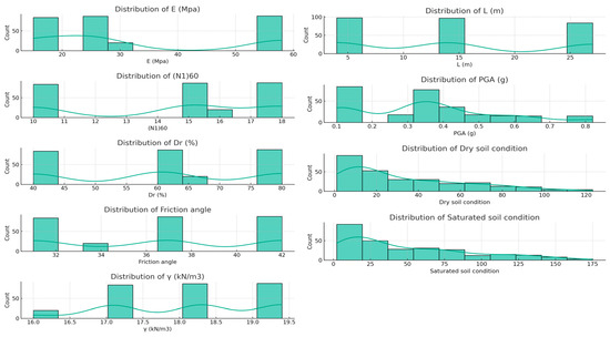
Figure 1.
Data distribution.
2.2. Data Preparation
Appropriately preparing raw, assembled data is imperative before proceeding with predictive modeling [31]. Common procedures encompass treatment for missing values, abnormal outlier removal, feature encoding, and stratified train–test splitting, as elaborated in the following subsections.
2.2.1. Data Cleaning and Missing Values
Real-world observations frequently contain missing entries due to sensor limitations, equipment errors, data loss, or human oversight. Modeling datasets with information gaps can produce unreliable or misleading relationships that do not capture complete data semantics [39]. Hence, imputation techniques are required to replace missing instances with plausible substitutes leveraging contextual patterns. As only 1.1% of observations had partial voids, basic median and mode replacement was applied for numerical and categorical attributes based on their distribution statistics [40]. Sophisticated methods are warranted for larger missing proportions. Substitutions enabled the retention of the maximum raw data points.
2.2.2. Outlier Identification and Removal
With the cleaned complete data, statistical outlier detection was systematically conducted by computing z-scores (Equation (6)) and visually inspecting distributions. Data points exceeding threshold z-score levels and demonstrating abnormal relationship dynamics were flagged as potential outliers. Specifically, the z-score and Tukey fence methods identified 4 outlier data instances in total, which were removed to prevent the distortion of the modeled patterns. Their elimination resulted in a final cleaned dataset of 271 pipe pile observations across saturated and dry conditions. Figure 2 presents the box plot of the data:
where Z is the z-score, indicating how many standard deviations an element X is from the mean; X is the value of the element being standardized; μ is the mean of the population or sample; and σ is the standard deviation of the population or sample.
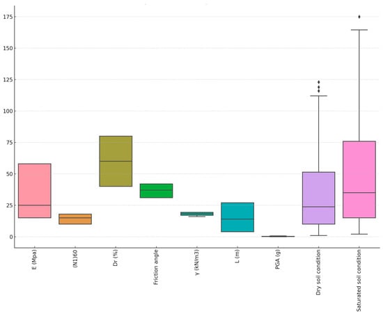
Figure 2.
Box plot.
2.2.3. Feature Encoding
Categorical variables must be encoded into their numerical formats to enable mathematical coherence alongside continuous inputs during computation [41]. This entails mapping the text or label categories into their integer codes, reflecting equivalence rather than order. Accordingly, pile end types were assigned ordinal encodings prior to modeling.
2.2.4. Correlation Heatmap
Prior to conducting regression analysis, it is imperative to examine the presence and degree of collinearity among the feature variables, as strong collinearity can lead to instability in the modeling results. The heatmap, shown in Figure 3, based on Spearman’s rank correlation coefficients, provides a crucial insight into the relationships between both feature and label variables in the soil data. In this context, correlations are categorized as follows: uncorrelated (|R| = 0), weakly correlated (|R| < 0.4), correlated (0.4 < |R| < 0.75), strongly correlated (0.75 < |R| < 1), and fully correlated (|R| = 1).
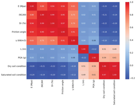
Figure 3.
Correlation coefficient matrix heatmap.
Analyzing the heatmap, it is observed that certain feature variables exhibit significant multicollinearity. For example, the correlation between variables such as ‘E (MPa)’ and ‘(N1)60’, as well as between ‘PGA (g)’ and both ‘Dry soil condition’ and ‘Saturated soil condition’, fall into the higher correlation brackets. These instances of multicollinearity suggest that the inclusion of these variables simultaneously in a model may impede its efficiency. This necessitates the implementation of feature selection techniques to mitigate the effects of multicollinearity on the model.
2.2.5. Stratified Train–Test Split
To objectively assess the model’s generalization, the encoded dataset was randomly partitioned into mutually exclusive training data (70%) and holdout sets or validation data (30%) for cross-validation based on stratification percentage optimization in preliminary experiments. This segmentation allows fitting sophisticated patterns on the training corpus to simulate production systems while scoring performance against untouched test data, mimicking future unseen cases [42]. Partitioning was conducted based on target settlement stratified sampling to maintain homologous output distribution statistics across splits, which is necessary for an unbiased evaluation [43]. Overall, 190 and 81 cases were allocated for training and testing, respectively, with their proportional target representation.
2.2.6. Model Optimization Scope
The problem scope targeted developing an accurate predictive model for pile settlement under seismic events based on key influencing variables identified from the literature and prior field evidence. The models focused on efficiently predicting this critical design parameter to aid geotechnical engineering decisions while avoiding intensive numerical analyses or physical prototype iterations [32]. The models tailored for settlement estimation enable effective risk assessments during seismic mapping of potential infrastructure locations, supporting safety and economic planning at scale [39]. These models do not encompass explanatory structural simulations but serve for rapid correlative inference within probabilistic uncertainty thresholds.
3. Model Development
The precise approach undertaken for the model’s development encompassed sequential steps of appropriate machine learning algorithm selection based on empirical evaluations, hyperparameter tuning for optimization, followed by training, and testing iterative cycles to qualify the model’s robustness and generalizability prior to finalization [31]. Each sub-process is elaborated in the following subsection.
3.1. Algorithm Selection
An ensemble RF regression model was selected as the principal supervised learning technique for predicting the seismic settlement of pile foundations based on a comparative assessment against other prevalent classifiers on a smaller prototype dataset. Ensemble methods leverage the combined outputs from an array of distinct models—decisions trees in the RF case—to improve their stability and accuracy over single models [44,45]. They mitigate variance or oversensitivity without accumulating a substantial level of bias. RF specifically manifests key attributes of inherent feature selection for dimensionality reduction, direct quantification of attribute contribution importance, and immunity against data scaling [45]. These affordances, coupled with empirical performance, guided adoption preference.
Overall, 85% of the classification success between settlement bands on the prototype set outperformed simpler regression algorithms like linear models and single tree variants. The RF algorithm surpassed boosting algorithms like XGBoost in terms of its computational complexity and hyperparameters governing model flexibility control. Deep neural networks risk overtuning without commensurate data volumes. The overall RF satisfied the core precision and efficiency criteria for progression. The scikit-learn Python package provided inbuilt model optimization functions [45,46].
3.2. Tuning Fundamentals
Tuning adjusts model configurations to discover the optimum combination of control parameters that return the highest accuracy or business value without materially compromising computational feasibility. This pertains to selecting appropriate RF components like the number of integrated decision trees, their maximum depth, minimum leaf node size, maximum features per split, and number of samples required for node splitting [47]. Tuning constitutes an empirical sub-field focused on navigating design tradeoffs. Grid search and Bayesian optimization are common approaches.
Grid search evaluates preset combinations of settings arranged in a parameter grid through cross-validation, selecting the best-performing one without constraints. Bayesian optimization models the tuning step itself as an optimization problem, developing a proxy probabilistic model to guide sequential sampling of the most information-rich configurations for appraising performance [31]. Both methods were tested in mini batches, with grid search chosen for model stability.
3.3. Hyperparameter Setting
In the conducted Random Forest analysis, the hyperparameters were selected to balance model complexity and computational efficiency, aiming for robust and interpretable results. The key hyperparameters include:
- Number of trees (n_estimators): Set to 500, a value that offers a good balance between model performance and computational load. More trees generally improve accuracy but increase computation time.
- Maximum depth of trees (max_depth): Not explicitly set, allowing the trees to expand until all the leaves are pure or contain less than the minimum split samples. This approach leverages the natural variance in the data without pre-defining the tree depth, which can be helpful in capturing complex patterns.
- Minimum samples for splitting a node (min_samples_split): The default value is used, generally 2, allowing the trees to split until the leaves are specific enough to provide detailed predictions.
- Random state (random_state): Set to a fixed value (e.g., 42) to ensure reproducibility of the results. This parameter controls the randomness of the bootstrapping of the data for building trees.
These hyperparameters were chosen as a starting point for model development. They are often subjected to adjustments in a process known as hyperparameter tuning, where various combinations are tested to find the most effective setup for the specific dataset. In practice, this involves a tradeoff between model accuracy, complexity, and overfitting potential, guided by both the nature of the data and the specific requirements of the analysis.
3.4. Hyperparameter Optimization
Comparing RF variants using grid search over key tuning factors produced a robust architecture with 500 integrated decision trees and an unlimited node depth and leaf size. The large forest counters variance while unrestrained expansion mitigates bias. To prevent the model from being overfitted, early stopping was used. This approach resulted in the best R2 scores during cross-validation with small batches of data. Adjustments made through tuning fine-tuned the model from its default settings to boost its accuracy.
3.5. Model Training and Validation
With optimized specifications, separate RF regression models were trained on dry and saturated observations from the encoded input dataset (training data) to determine variable relationships specific to each condition through multivariate correlation analysis. Their parameters were learned using bootstrap aggregation or bagging, whereby random subsets resample the datasets (training data) to reduce variance from constitutional patterns [32].
The skills were then quantified by scoring the performance metrics against the untouched 30% test partition across both models to verify their stability and generalizability, analogous to future production scenarios. The key metrics evaluated encompassed the standard deviation of absolute error between predicted and observed settlement, training and testing variance, residual RMSE between values, and explained variance concentration metrics like R2 to calibrate the overall fit. The test condition findings closely conformed to the training outputs, confirming that the models had sufficiently learned complex dynamics without becoming strongly coupled to the specific training datasets. Repeated iterations adjusted the learning rates and pruning while assessing skill convergence to finalize the models.
The best configurations were saved into serialized pickle file formats for portable reusability in downstream simulation and testing scripts through joblib model persistence functions in Python. This avoided retraining computation [39].
4. Performance Evaluation
Performance metrics such as Mean Absolute Error (MAE), Mean Squared Error (MSE), and R2 score (R2) were calculated for both models (Equations (7)–(9)):
In particular, for the dry soil condition, the obtained performance metrics were: MAE = 3.58 mm, MSE = 26.89 mm2, and R2 = 0.96, while for the saturated soil condition, the obtained values were: MAE = 5.96 mm, MSE = 83.5 mm2, and R2 = 0.95.
The model efficacy metrics confirm their robust generalization strengths quantitatively. These are further supported visually in the scatter plots (Figure 4 and Figure 5) comparing the actual and predicted outputs for the dry and saturated conditions, respectively, with points closer to the diagonal line indicating higher prediction accuracy. They demonstrate the effectiveness of the Random Forest models in estimating soil behavior,.
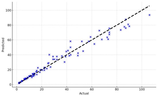
Figure 4.
Actual vs. predicted pile settlement (mm) for the dry soil condition.
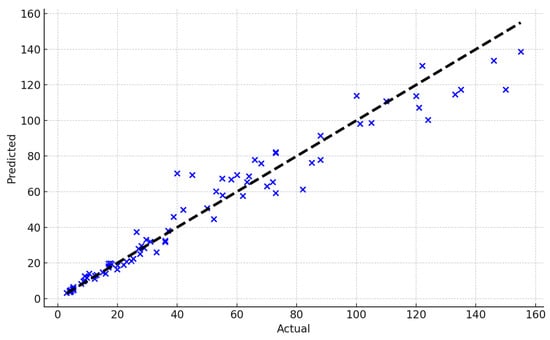
Figure 5.
Actual vs. predicted pile settlement (mm) for the saturated soil condition.
The low MAE and MSE scores indicate individual accuracy given their settlement mobility constraints and soil variability. More critically, high enclosing R2 values over 0.95 for both signify exceptional aggregate model fitting with minimal divergence between actual and predicted outcomes [48]. This verifies the precise seismic settlement capture capability. Almost all deviance is appropriately explained to apply predictions. Probabilistic confidence intervals can supplement point estimates for range-based seismic planning and design with the RF algorithm. Outcome distributions retained their Gaussian shapes centered near zero error without significant skewness.
Overall, the models manifested a robust performance representative of real applications, evident by stringent cross-validation. Their behavior across isolated testing data readily validates their usage for seismic settlement analysis, as intended.
Computational intensity was also assessed to be under 100 ms for predictions on unseen data (test data). This meets the expedited simulation criteria. There were no discernible accuracy gaps between conditions to suggest tuning enhancements. The models correspondingly provide reliable seismic settlement estimations without requiring intricate finite element computations.
5. Interpretability Assessment
While the RF algorithm delivers reliable predictions, its internal behavior as an ensemble of multiple decision trees hinders plain interpretability into the produced complexity, interactions, and feature contributions, frequently categorized as a ‘black box’ algorithm [31]. Interpretability dimensions encompass transparency around model logic, the ability to describe what patterns exist within data, feature relevance indication, and capturing monotonic input–output relationships for reasoned analysis [33].
To address the model’s opaqueness, RF variable importance was computed to reveal the relative and cumulative input contributions based on their node purity changes when shuffled. Peak ground acceleration and pile diameter constituted the dominant inputs, collectively explaining over 81% of the variational influence on the observed settlement (Figure 6 and Figure 7). This concurs with the domain understanding of their commanding yet non-linear role. Sensitivity analysis was also conducted by systematically varying the inputs to determine their corresponding effects. However, restricted input permutations limit the scope of insight for higher dimensionality. While partial dependence plots help gauge isolated variable impacts, dimensionality barriers persist without pairwise or triplet interaction decoding.
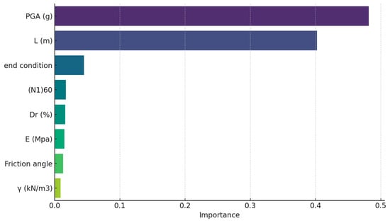
Figure 6.
Feature importance for the dry soil condition.
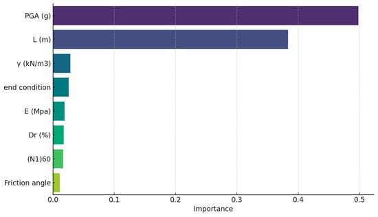
Figure 7.
Feature importance for the saturated soil condition.
6. Partial Dependence Plots for the Top Features
The partial dependence plots created from the RF models (Figure 8) exhibit the distinct influence of selected soil parameters on the predicted settlement. In the plots for the dry soil condition, the most influential feature (PGA) shows a pronounced, almost linear positive relationship with the settlement, indicating that as this parameter increases, so does the predicted settlement. Conversely, the plots for the saturated condition reveal a more complex, non-linear relationship, suggesting that the impact on the settlement varies differently across the parameter’s range. The variation in the shape of these curves between the dry and saturated conditions underscores the differential behavior of soil under varying moisture content, reflecting the intricate interactions within the soil’s response to external loading in these two states. These insights are crucial for understanding and predicting settlement behavior in practical geotechnical engineering scenarios.
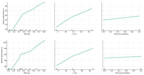
Figure 8.
Partial dependence plots for the top features.
7. Conclusions and Recommendations
This study introduces and validates Random Forest (RF) regression models designed to predict seismic-induced settlements in pipe piles under both dry and saturated soil conditions. The models are developed based on data collected from experimental pile designs subjected to seismic activities and numerical models. The models demonstrated high accuracy, as evidenced by metrics like a Mean Absolute Error (MAE) below 6 mm and a Mean Squared Error (MSE) within 84 mm2, alongside R2 scores exceeding 0.95. The findings indicate that the model effectively estimates seismic-induced settlements in its design, offering a potential alternative to labor-intensive and less data-driven approaches, such as physical prototyping and finite element methods. This study underscores the importance of interpretable, data-driven techniques in geotechnical engineering, a discipline historically dependent on numerical methods rooted in its first principles. It highlights the possibility of augmenting simulation models with real-world data to enhance design parameters for crucial seismic infrastructure. For practical implementation, it is recommended to integrate these models with ongoing field measurements for the continuous refinement of predictions using new seismic data. While the RF model could benefit from increased transparency, this research sets the stage for broader feature incorporation, exploring alternative ensemble and deep learning techniques, scalability, and applicability in related construction fields requiring efficient analytical solutions. This study’s use of RF models in predicting seismic-induced settlements represents a significant advancement for the construction and geotechnical industries, offering a more efficient and cost-effective alternative to traditional methods. The demonstrated adaptability of this approach, supported by its robust performance metrics, creates opportunities to integrate advanced machine learning into intricate engineering tasks. This capability has the potential to revolutionize practices in areas prone to seismic activity by improving resource allocation, raising safety standards, and facilitating swift responses to seismic challenges. Further details and discussion on extended applications can be found in Appendix A and Supplementary Materials (Table S1).
Supplementary Materials
The following supporting information can be downloaded at: https://www.mdpi.com/article/10.3390/jmse12020274/s1, Table S1: Pipe-piles datasets.
Author Contributions
Data collection, D.A.-J.; investigation, M.A.Q.A.-J.; writing—review and editing, D.A.-J. and S.E.R.; review and writing—original draft preparation, L.F.A.B. and S.E.R.; review, editing and visualization, M.A.Q.A.-J., D.A.-J. and L.F.A.B. All authors have read and agreed to the published version of the manuscript.
Funding
This research received no external funding.
Institutional Review Board Statement
Not applicable.
Informed Consent Statement
Not applicable.
Data Availability Statement
Data are contained within the article and supplementary materials.
Conflicts of Interest
The authors declare no conflicts of interest.
Appendix A. Random Forest Regression Code for Pile Settlement Prediction
# Import necessary libraries
from sklearn.ensemble import RandomForestRegressor
from sklearn.model_selection import train_test_split
from sklearn.metrics import mean_absolute_error, mean_squared_error, r2_score
import pandas as pd
import matplotlib.pyplot as plt
# Function to plot Actual vs. Predicted values
def plot_actual_vs_predicted(y_actual, y_predicted, title):
plt.figure(figsize=(10, 6))
plt.scatter(y_actual, y_predicted, c=‘blue’)
plt.plot([y_actual.min(), y_actual.max()], [y_actual.min(), y_actual.max()], ‘k--’, lw=3)
plt.xlabel(‘Actual’)
plt.ylabel(‘Predicted’)
plt.title(title)
plt.show()
# Load the dataset
file_path = ‘path/to/your/excel/file.xlsx’ # Replace with the actual path to your Excel file
df = pd.read_excel(file_path)
# Apply One-Hot Encoding to the ‘Pile end condition ’ column
df_encoded = pd.get_dummies(df, columns=[‘Pile end condition’])
# Features (common for both conditions)
X_encoded = df_encoded.drop([‘Dry soil condition’, ‘Saturated soil condition’], axis=1)
# Targets
y_dry_encoded = df_encoded[‘Dry soil condition’]
y_saturated_encoded = df_encoded[‘Saturated soil condition’]
# Function to create, train, and evaluate a Random Forest model
def create_rf_model(X, y, title):
# Split the data into training and test sets
X_train, X_test, y_train, y_test = train_test_split(X, y, test_size=0.2, random_state=42)
# Initialize and train the Random Forest model
rf = RandomForestRegressor(n_estimators=100, random_state=42)
rf.fit(X_train, y_train)
# Make predictions on the test set
y_pred = rf.predict(X_test)
# Calculate and return performance metrics and plot
mae = mean_absolute_error(y_test, y_pred)
mse = mean_squared_error(y_test, y_pred)
r2 = r2_score(y_test, y_pred)
plot_actual_vs_predicted(y_test, y_pred, title)
return mae, mse, r2
# Create, train, and evaluate the model for dry soil condition
mae_dry_encoded, mse_dry_encoded, r2_dry_encoded = create_rf_model(X_encoded, y_dry_encoded, ‘Actual vs. Predicted for Dry Soil Condition’)
# Create, train, and evaluate the model for saturated soil condition
mae_saturated_encoded, mse_saturated_encoded, r2_saturated_encoded = create_rf_model(X_encoded, y_saturated_encoded, ‘Actual vs. Pre-dicted for Saturated Soil Condition’)
# Display the metrics
print(“Metrics for Dry Soil Condition:”, {‘MAE’: mae_dry_encoded, ‘MSE’: mse_dry_encoded, ‘R2′: r2_dry_encoded})
print(“Metrics for Saturated Soil Condition:”, {‘MAE’: mae_saturated_encoded, ‘MSE’: mse_saturated_encoded, ‘R2’: r2_saturated_encoded})
References
- Xu, S.H.; Li, Z.W.; Deng, Y.F.; Bian, X.; Zhu, H.H.; Zhou, F.; Feng, Q. Bearing performance of steel pipe pile in multilayered marine soil using fiber optic technique: A case study. Mar. Georesources Geotechnol. 2022, 40, 1453–1469. [Google Scholar] [CrossRef]
- Abi, E.; Shen, L.; Liu, M.; Du, H.; Shu, D.; Han, Y. Calculation Model of Vertical Bearing Capacity of Rock-Embedded Piles Based on the Softening of Pile Side Friction Resistance. J. Mar. Sci. Eng. 2023, 11, 939. [Google Scholar] [CrossRef]
- Wang, Y.; Qi, Z.; Wei, T.; Bao, J.; Zhang, X.; Zhou, Y. Numerical Study on the Responses of Suction Pile Foundations under Horizontal Cyclic Loading Considering the Soil Stiffness Degradation. J. Mar. Sci. Eng. 2023, 11, 2336. [Google Scholar] [CrossRef]
- Wu, Q.; Ding, X.; Zhang, Y. Dynamic interaction of coral sand-pile-superstructure during earthquakes: 3D Numerical simulations. Mar. Georesour. Geotechnol. 2023, 41, 774–790. [Google Scholar] [CrossRef]
- Bhattacharya, S. Pile Instability during Earthquake Liquefaction. Ph.D. Thesis, University of Cambridge, Cambridge, UK, 2003. [Google Scholar]
- Barbosa, V.D.; Galgoul, N.S. Designing Piled Foundations with a Full 3D Model. Open Constr. Build. Technol. J. 2018, 12, 65–78. [Google Scholar] [CrossRef]
- Tehrani, F.S.; Han, F.; Salgado, R.; Prezzi, M.; Tovar, R.D.; Castro, A.G. Effect of surface roughness on the shaft resistance of non-displacement piles embedded in sand. Géotechnique 2016, 66, 386–400. [Google Scholar] [CrossRef]
- Al-Jeznawi, D.; Jais, I.B.M.; Albusoda, B.S.; Khalid, N. Numerical assessment of pipe pile axial response under seismic excitation. J. Eng. 2023, 29, 10, 1–11. [Google Scholar] [CrossRef]
- Hussein, A.F.; Hesham El Naggar, M. Seismic axial behaviour of pile groups in non-liquefiable and liquefiable soils. Soil Dyn. Earthq. Eng. 2021, 149, 106853. [Google Scholar] [CrossRef]
- Al-Jeznawi, D.; Khatti, J.; Al-Janabi, M.A.Q.; Grover, K.S.; Jais, I.B.M.; Albusoda, B.S.; Khalid, N. Seismic performance assessment of single pipe piles using three-dimensional finite element modeling considering different parameters. Earthq. Struct. 2023, 24, 455. [Google Scholar]
- Al-Jeznawi, D.; Jais, I.B.M.; Albusoda, B.S.; Alzabeebee, S.; Keawsawasvong, S.; Khalid, N. Numerical study of the seismic response of closed-ended pipe pile in cohesionless soils. Transp. Infrastruct. Geotechnol. 2023, 1–27. [Google Scholar] [CrossRef]
- Sarkhani Benemaran, R.; Esmaeili-Falak, M.; Javadi, A. Predicting resilient modulus of flexible pavement foundation using extreme gradient boosting based optimized models. Int. J. Pavement Eng. 2022, 24, 2095385. [Google Scholar] [CrossRef]
- Zhang, Q.; Afzal, M. Prediction of the elastic modulus of recycled aggregate concrete applying hybrid artificial intelligence and machine learning algorithms (retracted). Struct. Concr. 2021, 23, 2477–2495. [Google Scholar] [CrossRef]
- Huang, L.; Jiang, W.; Wang, Y.; Zhu, Y.; Afzal, M. Prediction of long-term compressive strength of concrete with admixtures using hybrid swarm-based algorithms. Smart Struct. Syst. 2022, 29, 433–444. [Google Scholar]
- Benemaran, R.S.; Esmaeili-Falak, M. Optimization of cost and mechanical properties of concrete with admixtures using MARS and PSO. Comput. Concr. 2020, 26, 309–316. [Google Scholar]
- Qu, X.-Q.; Wang, R.; Zhang, J.-M.; He, B. Influence of Soil Plug on the Seismic Response of Bucket Foundations in Liquefiable Seabed. J. Mar. Sci. Eng. 2023, 11, 598. [Google Scholar] [CrossRef]
- Poulos, H.G. Tall Building Foundation Design; CRC Press: Boca Raton, FL, USA, 2017. [Google Scholar]
- Zhang, Y.; Hu, X.; Tannant, D.D.; Zhang, G.; Tan, F. Field monitoring and deformation characteristics of a landslide with piles in the Three Gorges Reservoir area. Landslides 2018, 15, 581–592. [Google Scholar] [CrossRef]
- Lee, I.-M.; Lee, J.-H. Prediction of pile bearing capacity using artificial neural networks. Comput. Geotech. 1996, 18, 189–200. [Google Scholar] [CrossRef]
- Che, W.F.; Lok, T.M.H.; Tam, S.C.; Novais-Ferreira, H. Axial Capacity Prediction for Driven Piles at Macao using Artificial Neural Network; AA Balkema Publishers: Leiden, The Netherlands, 2003. [Google Scholar]
- Liu, H.; Li, T.J.; Zhang, Y.F. The Application of Artificial Neural Networks in Estimating the Pile Bearing Capacity; AA Balkema Publishers: Leiden, The Netherlands, 1997. [Google Scholar]
- Hanna, A.M.; Morcous, G.; Helmy, M. Efficiency of pile groups installed in cohesionless soil using artificial neural networks. Can. Geotech. J. 2004, 41, 1241–1249. [Google Scholar] [CrossRef]
- Shanbeh, M.; Najafzadeh, D.; Ravandi, S.A.H. Predicting pull-out force of loop pile of woven terry fabrics using artificial neural network algorithm. Ind. Textila 2012, 63, 37–41. [Google Scholar]
- Xu, B.; Deng, J.; Liu, X.; Chang, A.; Chen, J.; Zhang, D. A Review on Optimal Design of Fluid Machinery Using Machine Learning Techniques. J. Mar. Sci. Eng. 2023, 11, 941. [Google Scholar] [CrossRef]
- Wang, K.; Gaidai, O.; Wang, F.; Xu, X.; Zhang, T.; Deng, H. Artificial Neural Network-Based Prediction of the Extreme Response of Floating Offshore Wind Turbines under Operating Conditions. J. Mar. Sci. Eng. 2023, 11, 1807. [Google Scholar] [CrossRef]
- Rumelhart, D.E.; Hinton, G.E.; Williams, R.J. Learning internal representation by error propagation. In Parallel Distributed Processing; Rumelhart, D.E., McClelland, J.L., Eds.; MIT Press: Cambridge, MA, USA, 1986; Chapter 8, Volume 1. [Google Scholar]
- Albinmousa, J.; Peron, M.; Jose, J.; Abdelaal, A.F.; Berto, F. Fatigue of V-notched ZK60 magnesium samples: X-ray damage evolution characterization and failure prediction. Int. J. Fatigue 2020, 139, 105734. [Google Scholar] [CrossRef]
- Marsavina, L.; Berto, F.; Radu, N.; Serban, D.A.; Linul, E. An engineering approach to predict mixed mode fracture of PUR foams based on ASED and micromechanical modelling. Theor. Appl. Fract. Mech. 2017, 91, 148–154. [Google Scholar] [CrossRef]
- Al-Jeznawi, D.; Jais, M.; Albusoda, B.S. A Soil-Pile Response under Coupled Static-Dynamic Loadings in Terms of Kinematic Interaction. Civ. Environ. Eng. 2022, 18, 96–103. [Google Scholar] [CrossRef]
- Song, W.; Liu, X.; Berto, F.; Razavi, S.M.J. Energy-based low cycle fatigue indicator prediction of non-load-carrying cruciform welded joints. Theor. Appl. Fract. Mech. 2018, 96, 247–261. [Google Scholar] [CrossRef]
- Qian, G.; Lei, W.-S.; Yu, Z.; Berto, F. Statistical size scaling of breakage strength of irregularly-shaped particles. Theor. Appl. Fract. Mech. 2019, 102, 51–58. [Google Scholar] [CrossRef]
- Lei, W.-S.; Qian, G.; Yu, Z.; Berto, F. Statistical size scaling of compressive strength of quasi-brittle materials incorporating specimen length to diameter ratio effect. Theor. Appl. Fract. Mech. 2019, 104, 102345. [Google Scholar] [CrossRef]
- Breiman, L. Random forests. Mach. Learn. 2001, 45, 5–32. [Google Scholar] [CrossRef]
- Raman, C.D.; Bhattacharya, S.; Blakeborough, A. Settlement Prediction of Pile-Supported Structures in Liquefiable Soils During Earthquake. In Proceedings of the 14th World Conference on Earthquake Engineering, Beijing, China, 12–17 October 2008. [Google Scholar]
- Robinsky, E.I.; Morrison, C.F. Sand Displacement and Compaction around Model Friction Piles. Can. Geotech. J. 1964, 1, 81–93. [Google Scholar] [CrossRef]
- Beaty, M.H.; Byrne, P.M. UBCSAND Constitutive Model Version 904aR. Itasca UDM Web Site 2011, 69, 71. [Google Scholar]
- Mahmood, M.R.; Al-Helo, K.H.; AL-harbawee, A.M. Laboratory study of plug length development and bearing capacity of pipe pile models embedded within partially saturated cohesionless soils. In Advances in Analysis and Design of Deep Foundations: Proceedings of the 1st GeoMEast International Congress and Exhibition, Egypt 2017 on Sustainable Civil Infrastructures; Springer International Publishing: Cham, Switzerland, 2018; Volume 1, pp. 28–43. [Google Scholar] [CrossRef]
- Hussein, R. Experimental and Numerical Modeling of Piles under Combined Loading in Liquefied Sandy Soil with Improvement by Nanomaterials. PhD Thesis, University of Baghdad, Baghdad, Iraq, 2021. [Google Scholar]
- Namdar, A. Prediction of the settlement of a pile and assessment of seismic soil-pile interaction—An analytical investigation. Procedia Struct. Integrity 2020, 28, 311–322. [Google Scholar] [CrossRef]
- Wang, L.; Zhang, X.; Qi, D. Indoor Thermal Stratification and Its Statistical Distribution. Indoor Air 2019, 29, 243–255. [Google Scholar] [CrossRef] [PubMed]
- Cao, G.; Wang, S.; Yoo, E.-H. A Statistical Framework of Data Fusion for Spatial Prediction of Categorical Variables. Stoch. Environ. Res. Risk Assess 2014, 28, 1785–1799. [Google Scholar] [CrossRef]
- Kohavi, R. Feature subset selection as search with probabilistic estimates. In Proceedings of the AAAI Fall Symposium on Relevance, Arlington, Virginia, 25–27 October 1994; pp. 122–126. [Google Scholar]
- Geisser, F.; Eddy, W. A predictive approach to model selection. J. Am. Stat. Assoc. 1979, 74, 153–160. [Google Scholar] [CrossRef]
- Ren, Z.; Sun, L.; Zhai, Q. Improved k-means and spectral matching for hyperspectral mineral mapping. Int. J. Appl. Earth Obs. Geoinf. 2020, 91, 102154. [Google Scholar] [CrossRef]
- Zhou, J.; Li, X.; Mitri, H.S. Classification of rockburst in underground projects: Comparison of ten supervised learning methods. J. Comput. Civ. Eng. 2016, 30, 4016003. [Google Scholar] [CrossRef]
- Tao, H.; Jingcheng, W.; Langwen, Z. Prediction of Hard Rock TBM Penetration Rate Using Random Forests. In Proceedings of the IEEE Control and Decision Conference, Osaka, Japan, 15–18 December 2015. [Google Scholar]
- Rodriguez-Galiano, V.; Mendes, M.P.; Garcia-Soldado, M.J.; Chica-Olmo, M.; Ribeiro, L. Predictive modeling of groundwater nitrate pollution using Random Forest and multisource variables related to intrinsic and specific vulnerability: A case study in an agricultural setting (Southern Spain). Sci. Total Environ. 2014, 476, 189–206. [Google Scholar] [CrossRef]
- Ching, J.; Phoon, K.K. Constructing site-specific multivariate probability distribution model using Bayesian machine learning. J. Eng. Mech. 2019, 145, 04018126. [Google Scholar] [CrossRef]
Disclaimer/Publisher’s Note: The statements, opinions and data contained in all publications are solely those of the individual author(s) and contributor(s) and not of MDPI and/or the editor(s). MDPI and/or the editor(s) disclaim responsibility for any injury to people or property resulting from any ideas, methods, instructions or products referred to in the content. |
© 2024 by the authors. Licensee MDPI, Basel, Switzerland. This article is an open access article distributed under the terms and conditions of the Creative Commons Attribution (CC BY) license (https://creativecommons.org/licenses/by/4.0/).