1. Introduction
The accurate determination of a vessel’s main particulars holds paramount significance in the initial design phase of naval architecture, as these values serve as foundational parameters shaping the vessel’s overall characteristics. However, the complexity associated with deriving these particulars arises from a myriad of interrelated factors, rendering the task intricate and challenging.
Traditionally, the vessel’s main particulars were determined in the first iteration of the design spiral developed by J.H. Evans [
1], also called the concept phase. As the design continued to develop through the design spiral, the main particulars and the rest of the design would go through the next phase, called preliminary design, as stated by Papanikolaou [
2]. When starting the concept design phase, engineers usually begin with a comparison with similar already-existing vessels. For that purpose, statistical, rational, and empirical methods based on comparative data from similar ships were developed. Watson has developed design formulas based on which the main ship dimensions can be estimated [
3]. While investigating ship hull performance and the effect of main ship dimensions on weight, Strohbusch [
4] has explored and developed hull form coefficients and ratios of main dimensions for merchant ships. Watson later updated his formulas [
5], while Strohbusch’s approach was further developed by Papanikolaou [
2]. Specifically, the main dimensions of container ships, especially their length, are estimated based on cargo capacity parameters such as required deadweight, hold, or TEU capacity [
2,
6]. Similar to other merchant ships, in the phase of container ship concept design, the estimation of main dimensions is based on linear or nonlinear equations. These equations are derived from methodologies that utilize a database of previously constructed ships. Piko [
7] used a database of container ships built before 1980 to develop equations through a nonlinear regression methodology, employing deadweight capacity as an input. Papanikolau [
2] also utilized nonlinear regression methods, using data from container ships built before 2005, with deadweight capacity as the input in his research. Kristensen [
8] employed a second-degree polynomial and linear power regression method with a more recent database of container ships built before 2013. In his case, the input criterion was the TEU number.
With the advancement of artificial neural networks (ANN), scientists have increasingly utilized them to estimate the values that are crucial in ship design. Artificial neural networks can analyze data based on datasets; however, a limitation in the marine industry is the scarcity of available data. This limitation narrows the scope of areas that can be effectively analyzed using ANN, particularly to achieve high-quality results, as identified in [
9]; therefore, some of the primary research areas include main engine power, fuel consumption, resistance, and main dimensions, as explored in various specific research studies.
For instance, in [
10], scientists introduced a model that utilizes a combination of artificial neural networks (ANN) and multi-regression (MR) techniques to estimate a ship’s power and fuel consumption. This model was employed to predict potential fuel savings, and the results indicate that such a model can also play a crucial role in developing decision support systems (DSS) to maximize a ship’s energy efficiency. In [
11], a regression model utilizing an artificial neural network (ANN) approach was proposed to predict ship performance, specifically focusing on the fuel consumption of the vessel’s main engine. The authors drew several conclusions from their research. They found that sigmoid and tangent sigmoid functions exhibit high and stable regression values, even with a small number of hidden layers and neurons. In contrast, the ReLU function requires an adequate number of hidden layers and neurons to achieve high and stable regression values. Regression analysis using ANN becomes essential for predicting ship fuel consumption when dealing with nonlinear relationships between input and output variables. The conclusion is that regression analysis using ANN can effectively and accurately predict ship performance, serving as a complex and real-time model for the future of the shipping and marine industry.
A specific study conducted by Alkan et al. [
12] involved the analysis of initial stability parameters in fishing vessels using neural networks. Parameters such as the vertical center of gravity (KG), height of the transverse metacenter above the keel (KM), and vertical center of buoyancy (KB) were calculated with high accuracy levels when compared to the actual ship data. The added resistance coefficient was also examined through the application of ANN [
13]. A formula was developed and presented using ANN, showcasing practical applicability at the preliminary design stage. Similar to other ANN analyses, the limiting factor in this study was the dataset.
Analysis of the main dimensions has been conducted in multiple studies [
14,
15,
16]. In [
14], a method was proposed to determine the initial main particulars of chemical tankers. The study demonstrated that the LM algorithm achieved the best results, employing 13 hidden neurons. In [
15], researchers analyzed the main particulars of 250 container ships using MLP and GBT ML algorithms. Machine-learning-based models, such as those developed in this research, could be utilized by engineers in the preliminary design stages. Artificial neural networks were used in [
16] to analyze container ship length. Equations were developed to estimate the length between perpendiculars (Lpp) based on container number and ship velocity (v).
All the methods used so far rely on a dataset, and consequently, they are heavily limited by the size of that dataset. A large amount of data is available for typical types of ships, usually limited to specific values like main particulars. Other values, such as ship coefficients, resistance, fuel capacity, or information about crucial systems, are either unavailable or hard to obtain. Another influencing factor is the quality of the gathered data for the dataset, which significantly impacts the results of the methodology used. Therefore, the available data and their quality can be major constraints on the values that can be analyzed and used in ship design. This is especially problematic for specialized types of ships, such as those used for special operations, research vessels, submarines, and unmanned underwater vehicles (more specifically, the subcategory of underwater autonomous vehicles). Hence, this research aimed to establish an ML methodology that will overcome the lack of real-world data by using synthetic data to improve the quality of the ML-based model’s performance.
The main point of novelty of this research lies in answering the following research questions:
RQ1—Can quality synthetic data be generated from a relatively small dataset regarding container ships, using the limited probability density functions available to such modelling?
RQ2—Can such synthetic data be used to improve the performance of the model when regressed using the multilayer perceptron (MLP) method, in comparison to a model trained on just the original data?
RQ3—Is the improvement, observed across multiple metrics, equal across all targets in the dataset, or does it vary per target?
This study will first present the used methodology, focusing on the description of the dataset, followed by the techniques of data analysis and synthesis of that data. Finally, the regression methodology will be given a brief description. The results obtained with the described methodology are presented in the following section, they are discussed, and finally, the conclusions are drawn in the final section of the paper.
2. Methodology
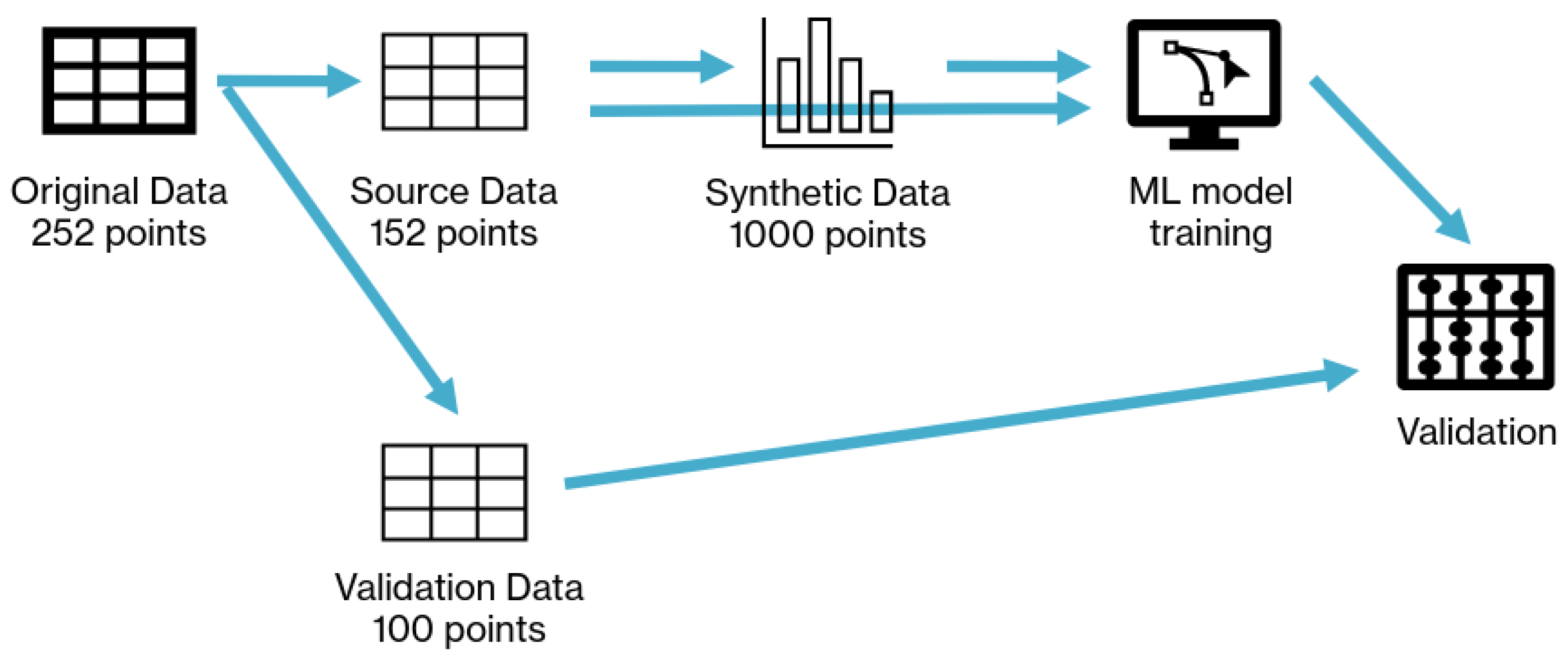
The approach used in this research is to test whether synthetically generated data points can be used to improve the performance of limited datasets. This study serves as a continuation and complement to the earlier research [
15], where the established database will be utilized as the foundation for this article. The original dataset is separated into two—the validation and training sets. The former set will be used for two purposes—the first is training the models based on the original data, while the second is the generation of the synthetic data. In addition to the original data-based models, additional models are developed based on the synthetic data, for performance comparison. Both of the models will finally be evaluated on the validation set. The original data consisting of 252 points is split into the source data for synthetic data generation and validation data. The validation data are left aside, while the source data are used for synthetic data model training, and it generates a total of 1000 additional data points. These synthetic data points are mixed with the original 152 source data points, and the models are trained with them, as well as just the source data without added synthetic data. These models are then evaluated on the original validation data. This process is presented in
Figure 1.
2.1. Dataset Description
The dataset is split into 152 data points for the training and 100 points for the validation. The 152 points will be the basis for the generation of the synthetic data and train the original data models for comparison. The dataset consists of 11 variables, 2 of which will be used as inputs and 9 which will be model outputs. The regression technique that will be used and described in the following sections only predicts a single value as its output. Because of that, a separate model must be developed for each of the outputs. The nine elements of the dataset used as outputs are:
The two inputs used are number of TEU (TEU) and speed (V). The class databases used in the creation of the dataset are DNV, Lloyd’s, and Bureau Veritas [
15].
2.2. Generations of Synthetic Data Points
The method used in this research for obtaining synthetic data points is copula. The implementation of the copula method this research uses is GaussianCopula from the Synthetic Data Vault (SDV) [
17]. The method works by generating a hypercube with the dimensions of
, where
d is equal to how many variables are present in the dataset. For the previously described dataset used in this research, the copula method will create a hypercube of dimensions
. Then, the method determines copulas. These copulas are equations that map each of the variable vectors in the original dataset to the hypercube. This mapping is done in such a way that the statistical distribution of the original variable is transformed into a uniform distribution, in which each value has the same probability of being randomly selected. This equation is created using a Taylor series. Once these equations are determined, they can be inverted. This determines the main application of the copula method. Once the hypercube and the equations are created, random values can be generated uniformly within the hypercube space. When this data vector from the hypercube is transformed back to the original data space, due to the nature of the inverted copula equation, the transformed values should retain the probability density function of the original data [
18].
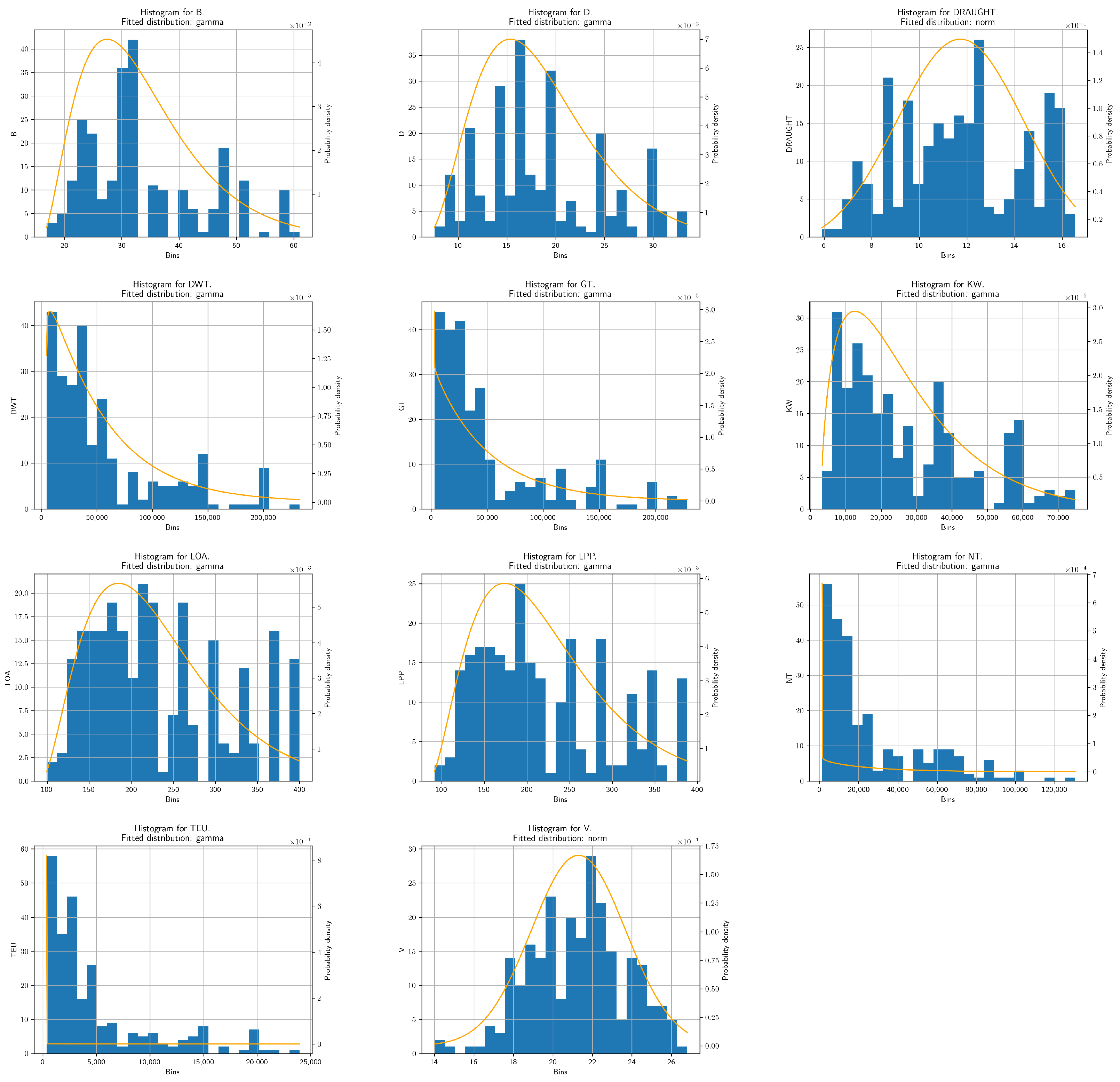
As can be seen from the name of the applied method—GaussianCopula (GC)—the method assumes that the original data are normally distributed. Not all data follow a normal distribution, which is why GC can also be used with the assumption that the data follow some other common distributions. These distributions are the beta distribution, uniform, gamma, and truncated normal distribution [
19]. Because of this, the first step in creating the synthetic data is to determine which of the possible distributions is the best fit to the original data variables. This is achieved using the Kolmogorov–Smirnoff (KS) test. If we assume the original distribution function of the variable is defined as
, where
is the observed variable, then the empirical distribution function
can be defined as the ratio of the number of elements smaller than
x to the total number of elements in the data vector, or [
20]:
If the probability density function that is being tested (for example normal distribution) is defined as
, following the same equation, then the KS statistic can be defined as the supremum of the distances [
21]:
By testing against all possible distributions, we can determine the one that has the lowest difference relative to the real data distribution.
One of the key concerns that need to be addressed when synthetic data are used, is the learning limitations. The synthetic data are not completely new data introduced to the dataset but are instead derived from the descriptive statistics of the original data. Because of this, there are limits to the amount of data that can be generated before experiencing issues such as re-learning the same data points and mode collapse. The main issue is the bias towards the original data set, which is used as the basis of the synthetic data. The models trained with synthetic data provided from the original data may have a poorer generalization performance on new data, compared to actually collecting and training the models with new data.
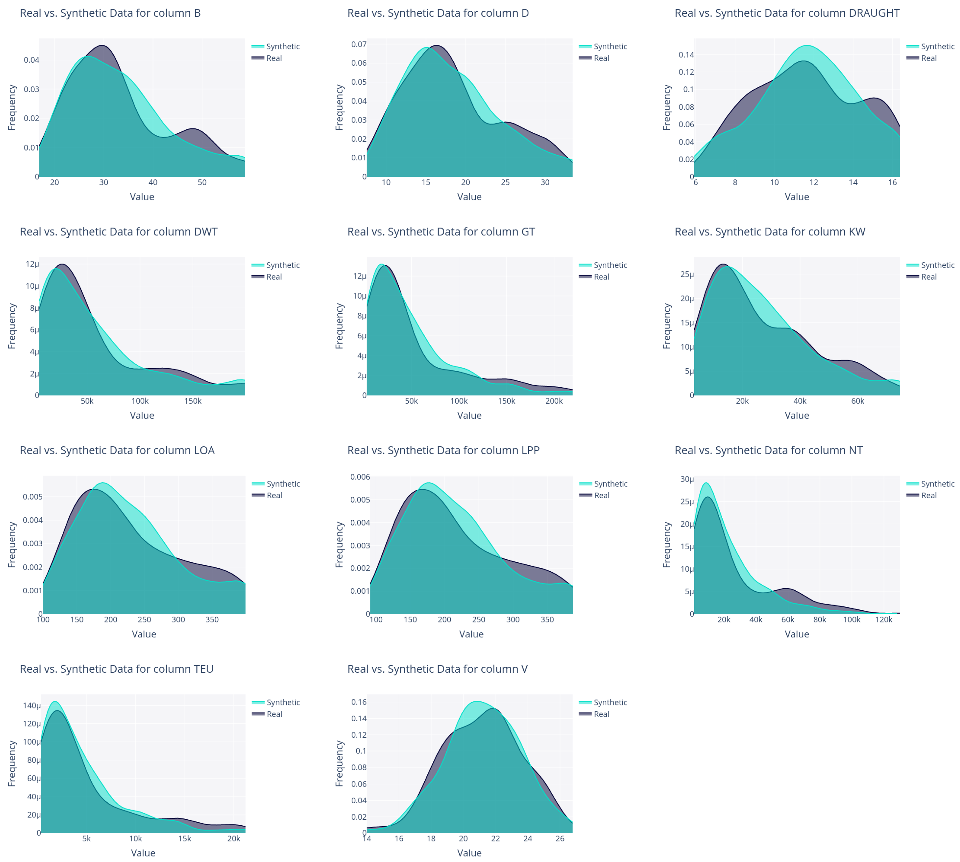
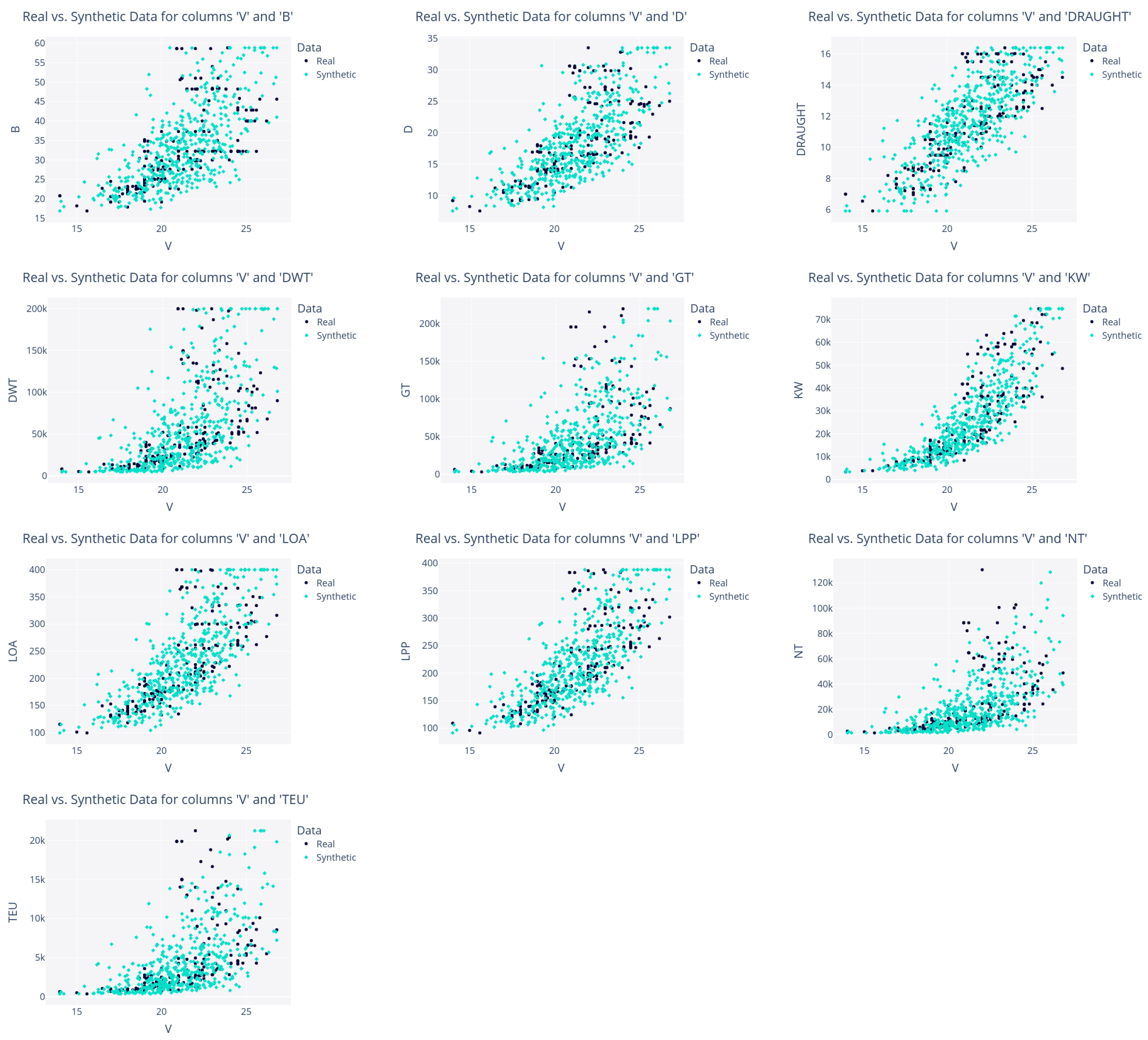
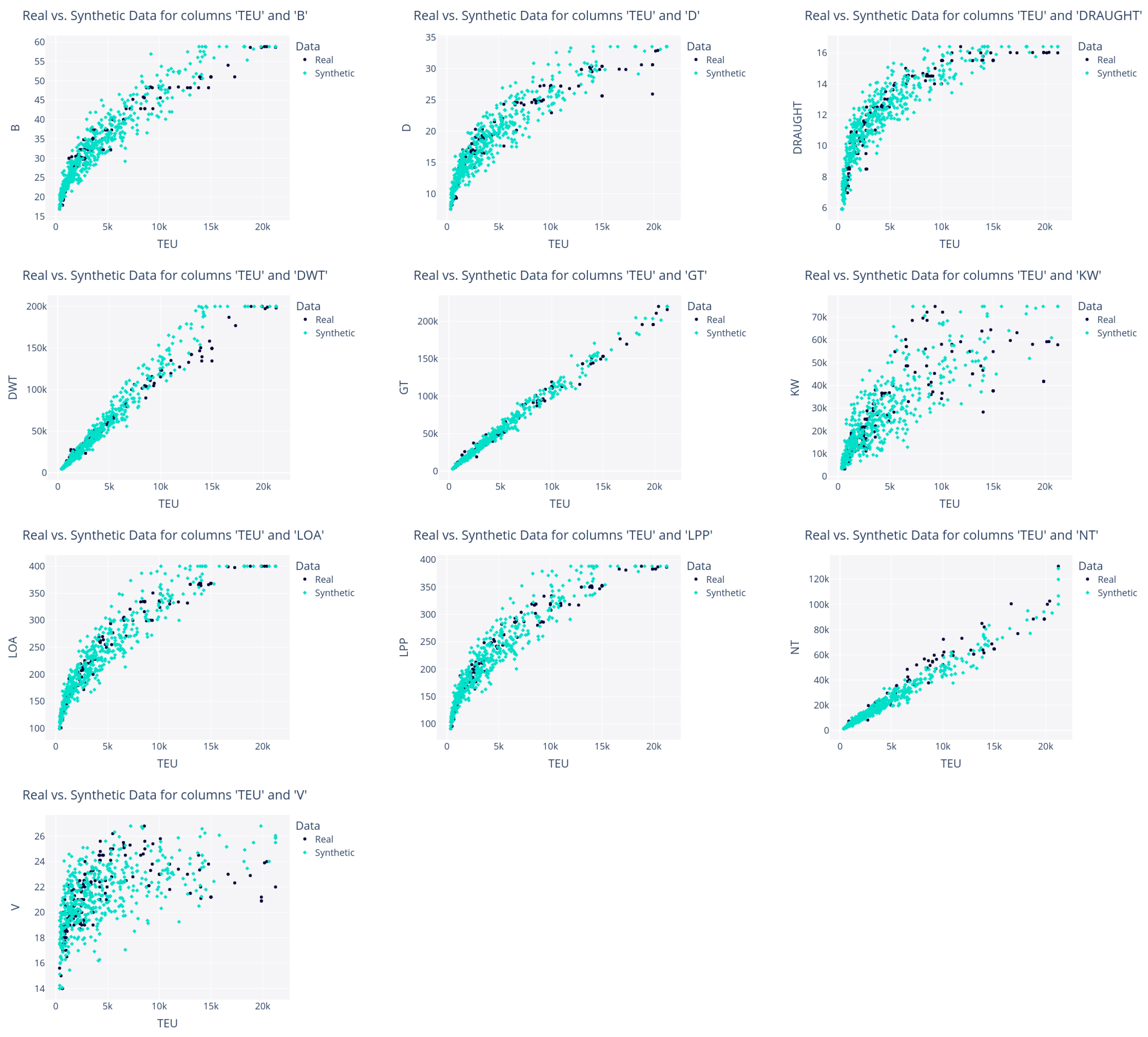
Another concern with synthetic data is the generation of infeasible designs. As main particulars are calculated using random selection, not all sets of values may give realistic main particulars—for example, a very large LPP combined with a shallow draught and a small B. To avoid extremely large discrepancies and impossible values, the synthetic data are limited to the range of values equal to the range of values contained in the original dataset. As that may still generate unrealistic main particulars, it is important to note that synthetic data in the given use-case is not meant to create realistic values. It is simply used to fill out the distributions of the original data and address possible gaps (visible in
Figure 2). This process should allow for the creation of more robust and precise models for the points which were not necessarily contained in the dataset, as well as smooth out the probability density functions, which are utilized as a key factor in modelling using statistical ML-based methods such as the one used in this research. The result of this “filling out” procedure will be shown in the figures showing data pairs and the comparison of probability density functions for real and synthetic data.
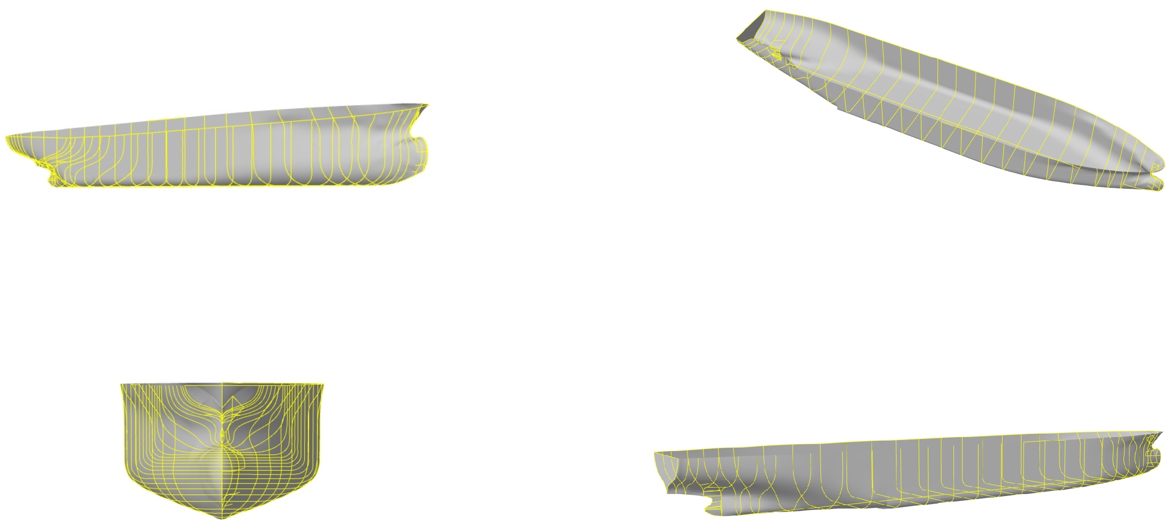
To assist in the visualization of the created data points, the authors have randomly selected one of the synthetic data points. Using the synthetic values as the main particulars of a vessel design, the ship form given in
Figure 3 was created, using pre-existing ship form lines adjusted to the main particulars obtained with the synthetic data method. Observing this form, it can be seen that the synthetic data values can be used for the creation of realistic vessels.
2.3. Regression Methodology
The regression test is performed using a multilayer perceptron (MLP) artificial neural network (ANN). This ANN is constructed from neurons arranged in three layers. These are the output and input layers, with additional “hidden” layers in between them (at least one). A neuron is connected to all the neurons of the following layers. The input layer consists of neurons whose number is equal to the variables in the dataset, and the output layer consists of a single neuron. The number of neurons in the hidden layers is arbitrary. The network works by taking each row in the dataset, defined as
, and using it as the input. These values are then propagated through the network by calculating the values of neurons. Each neuron value is calculated by taking the value of each neuron
(
i being the neuron, and
j being the layer) in the previous layer and multiplying it by the weight value
of the connection between the two neurons [
22]:
with
N being the number of neurons preceding it. This process is repeated until the output neuron is reached. This output value can be defined as the predicted value
. Comparing that to the real value of the output correlated to the data point
, defined as
, we can obtain the current error of the neural network for that data point. If we define
M as the number of data points in the training set, then the error of the network in the current iteration of training can be defined as [
23]:
The model is developed by adjusting connection weights proportionally to the error gradient, from the initial randomly set values. By repeating this process multiple times, the
will be minimized, theoretically obtaining a well-performing model [
24].
The values of the weights are the parameters of the network. In addition to those parameters, values exist within the network that define the architecture of the network—which are referred to as the hyperparameters of the network. These are the number of layers and the number of neurons in each layer, the activation function (value that adjusts the value of neurons to control the output range), regularization parameter L2 (parameter that controls the influence of the better correlating values), the learning rate (factor controlling the speed at which the weights are adjusted, as well as the type of adjustment), and solver (algorithm that calculates the weight adjustments) [
25]. In the presented research, these values are adjusted using the grid search (GS) algorithm. GS is a simple algorithm that tests all the possible combinations of the hyperparameters given as inputs. The possible values of hyperparameters of the MLP that were used in this research are given in
Table 1. The amount of neurons per layer indicates the number of neurons in each of the layers of the neural network, with more neurons indicating a more complex network. More complex networks show better performance when complex problems are modeled, but significantly raise the time necessary for model training, due to the larger number of weight adjustments that are necessary—as the number of connections between two layers of size
n is equal to
. Each of the neurons will perform a simple summation of
n weights, multiplied by
n results of the output neurons, and then processed with the activation function. The activation functions are simple, so their complexity can be assumed to be
, resulting in a total complexity of
. Still, as for the trained network,
n is a constant. Considering that the architecture was already decided, the complexity of a neuron can be simplified to
.
It can be seen that a relatively large number of layers was used in the network configurations. The training of the networks was performed using the Bura Supercomputer, available at the University of Rijeka, and because using larger networks did not present a significant time impact, the authors decided to explore the larger networks as well, in the hopes of obtaining better-performing models. Still, such large networks may not be necessary for the model regression.
Each of the obtained models from this procedure is evaluated on the separate test set (20% of the training set), with two values to determine the performance of the model on unseen data, with these values representing the metric known as the coefficient of determination (
) and the
(mean absolute percentage error).
shows how well the variance is represented between the predicted and original data and is calculated as [
26]:
The total value of
essentially explains the amount of variance from the original data that is explained in the predicted data. The best value of
is found when all of the variance is explained between the original and generated datasets.
is the average absolute error, expressed as the percentage. It has been selected due to the multiple values with different ranges used as outputs. Due to this, using an error normalized to the range will allow for a simpler comparison between results.
is calculated as [
27]:
4. Discussion
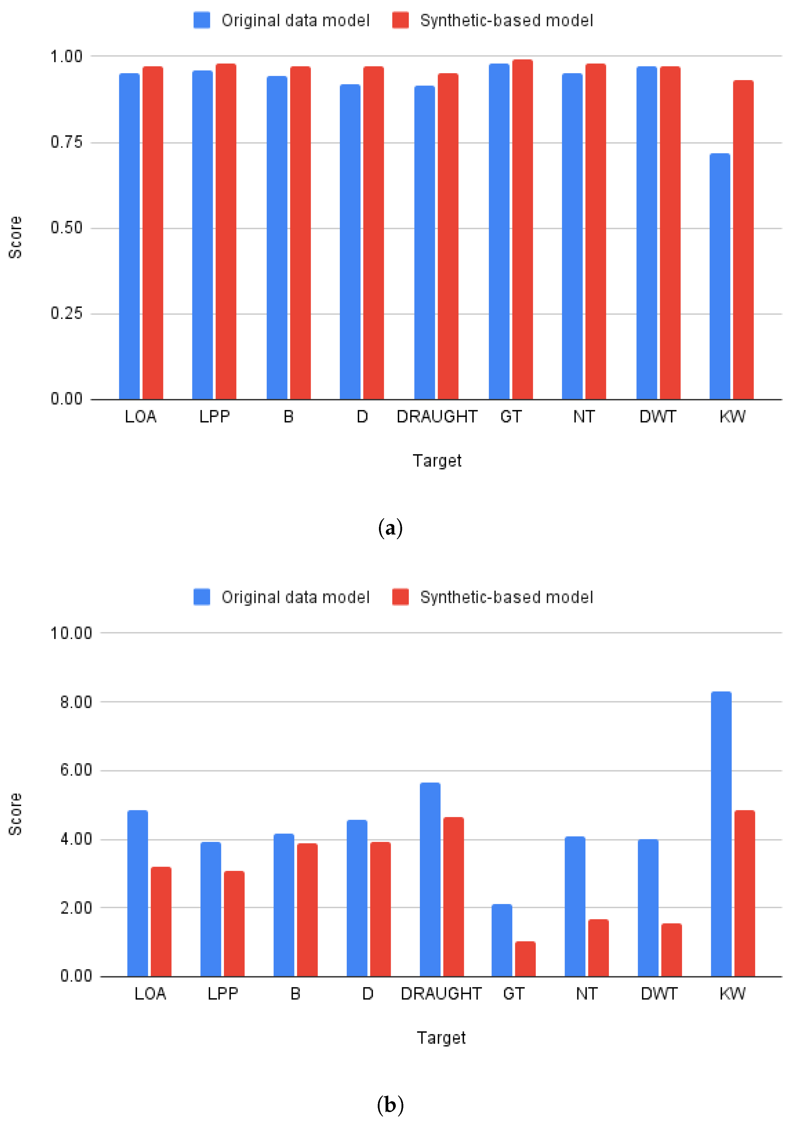
There are multiple points to the discussion of the achieved results. The first, and most important, element of note is that the models that utilize synthetic data for regression modelling achieve higher scores on the targeted outputs when compared to the scores achieved by models that were trained by fewer, original, data points. This is visible for all of the presented data points, with the sole exception of the DWT target, which achieved an equal score when evaluated with —but still showed improvement in the metric, which dropped from 4.02% to 1.53%.
From the ML perspective, it is interesting to note how different architectures were found to perform best between the two datasets. This was the case even though there was high similarity between datasets, as shown in
Figure 4,
Figure 5 and
Figure 6. This behavior indicates that despite the similarities between datasets shown in the current analysis of the data, there are underlying differences in the data hyperspace that are not captured with the analysis. It can be concluded that this means that performing the GS procedure from the start for different data models is necessary, and simply transferring model architectures between original and synthetic datasets is not applicable.
Performance between the training sets and the test set seems to be a good indication of the final model performance. This is best seen in the case of the KW output—where the test performance on original data shows an of 0.78 and of 0.91 for synthetic test data. This respectively translates to values of 0.72 and 0.93 for the real and synthetic models on validation data. Of course, validating data against a third dataset (in the presented work referred to as the validation dataset), which is unseen by both the synthesizing and regression models, is crucial. Still, there are similarities between the performance shown on test and validation sets, which allowed the models that were selected based on their test performance to show themselves to perform well in the validation step. This leads to potential time savings in this methodology, due to avoiding the need to test multiple models for each of the targets.
Finally, most of the models achieved with synthetic data using the described methodology are high performing enough to be considered for use in practical applications. The models that achieved performance higher than 0.95 are LOA, LPP, B, D, DRAUGHT, GT, NT, and DWT—in other words, all models except the KW model. If we evaluate the models using , all of the models trained on synthetic data achieve the condition of having an error lower than 5%. It should be noted that most of the original data models (the exceptions being DRAUGHT and KW) also achieve scores that are satisfactory according to the given conditions. Still, due to the relative simplicity of synthetic data application, and the low computational cost of the procedure, the obtained improvements indicate that such a methodology could prove to be useful in gaining additional performance from data-driven ML-based models.
5. Conclusions
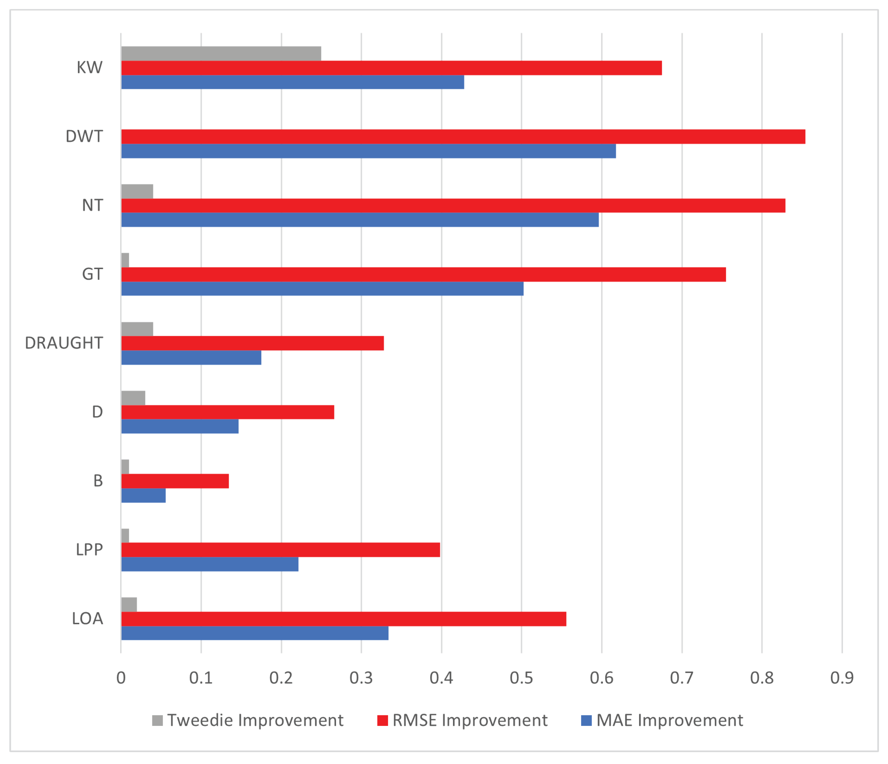
The presented research attempted to demonstrate the ability to improve the performance in main ship particular modelling through the use of synthetic data generation techniques. It used a previously collected dataset of container ship particulars to generate models based on just the original data and models based on a synthetic data-enhanced dataset, comparing the two approaches. Comparing the performance of models based on original and synthetic data on the separate validation part of the dataset, the improvement in regression quality is shown across almost all of the targets. Various ranges of improvement are present, from essentially the same performance (e.g., DWT evaluated with ) to significant improvement (e.g., KW improving the metric from 0.72 to 0.93 and dropping the from 8.29 to 4.86). None of the values have shown a drop in scores when synthetic data was introduced into the modelling process, indicating the synthesizing process, at worst, does not hurt the performance of the data.
The obtained results point towards the fact that it is possible to improve the design of main ship particulars using synthetic data. The main benefit of this lies in cases such as ship modelling, where large datasets cannot be collected from real-world data, due to a large amount of data points simply not existing. The fact that synthetic data generation is computationally cheap, especially in comparison to the actual regression modelling, has to be considered. This means that adding synthesis in the process of AI modelling may be a good idea, as it will not harm the performance but may significantly improve it.
The results allow us to address the original research questions posed at the introduction of this research. (RQ1) Yes, the generation of high-similarity synthetic data is possible, based on only 152 randomly selected original data points. (RQ2) The improvement in scores is apparent across all targets for models trained with the synthetic data combined with the original data. (RQ3) The improvement is not uniform across all targets, with different targets showing different levels of improvement depending on the observed metric.
Based on these findings, it can be concluded that an extended dataset augmented with synthetic data and analyzed using artificial neural networks (ANN) can yield favorable results. These outcomes are valuable for early-stage ship design, facilitating the estimation of main particulars. In ship design, access to large quantities of data is often limited. This paper demonstrates that even in such cases, ANN can be effectively employed by incorporating synthetic data. This approach proves especially beneficial for designing nonstandard ship types, such as ships intended for special purposes.
The limitations of the work lay in the fact that the research is performed on a relatively small dataset, which is focused on container vessels, so it is not possible to securely claim the possibility of generalizing the used approach on other vessel types. This should be addressed through the further testing of the described approach on different vessel types—on their own, as well as with datasets combining the main particulars of different vessel types. Two more limitations arise from the usage of synthetic data. First is the lack of real, new, data in the dataset—meaning that data points obtained from newly created vessels may not provide good results when evaluated with the created models. This limitation cannot be directly addressed at this time, as it could take years to collect additional data points from newly created container vessels, especially ones that differ significantly from existing ones. The second limitation is that as the models are not constrained to realistic proportions, the main particulars obtained in the synthesis process may not be realistic. While this is not an issue for the current study, it presents a limitation for the use of synthetic models such as GC, which are not able to generate realistic main particulars—and more advanced techniques such as custom deep convolutional generative adversarial networks should be applied if that is the goal, which may be an element of future work in this field. While it may be argued that the values obtained from ANN, despite fitting the original dataset well, may not be precise enough, it needs to be stressed that the developed work is mainly meant as an expert support system, which can provide starting values for further refinement by professionals with experience in the field. Future work may also include the use of the original and synthetic datasets presented in this study to create better models. The focus should be given to explainable AI techniques, in which models can be further analyzed and the logic behind them investigated. The importance of this lies in the simpler presentation and integration of created AI models into the actual workflow of researchers and engineers.


