Online Data-Driven Integrated Prediction Model for Ship Motion Based on Data Augmentation and Filtering Decomposition and Time-Varying Neural Network

Abstract

Online prediction for ship motion with strong nonlinear characteristics under harsh sea states will significantly reduce the damage of large accidents. Therefore, an integrated ship motion online prediction model consisting of a data augmentation algorithm based on the Improved Temporal Convolutional Network and Time Generative Adversarial Network (ITCN-TGAN), and an Improved Empirical Mode Decomposition (IEMD) and a Time-Varying Neural Network based on Global Time Pattern Attention (GTPA-TNN), is proposed in this article. The results of the validation tests in which the container ship KCS is taken as the example show that the synthetic data generated by ITCN-TGAN based on the dataset with few nonlinear samples are very similar to the original data, which proves that the synthetic data have high authenticity and can be used as training data to reduce the sampling cost; the input signal is decomposed into multiple Intrinsic Mode Functions (IMFs) by IEMD without noise diffusion, an endpoint effect, or mode mixing occurring in it, which indirectly improved the accuracy; and the dynamic sliding window adaptively adjusts the input sequence length according to the waveform characteristics to improve the computational stability of the model, the accuracy of GTPA-TNN can maintain a high level during the prediction period in various working conditions, and the error distribution is almost the same, which suggests that the integrated model has strong robustness and can realize the goal of online prediction of ship motion under harsh sea conditions.

1. Introduction

Influenced by the waves and currents, a ship will be in a violent swaying motion when sailing under harsh sea conditions, which can easily cause damage to marine equipment and mechanical components. Therefore, accurate online prediction for ship motion in a short amount of time can give the staff a certain reaction time, reduce the damage to equipment, and avoid causing the ship to sink, which can significantly reduce the risk of an accident.

At the initial stage of the study of ship motion, researchers tried to solve the ship motion equation or establish a linear autoregressive model to predict it. Prediction models with a static structure such as Kalman filtering [1,2,3] or sliding autoregressive models [4,5,6] are widely used. However, due to multiple non-stationary external factors such as wind, waves, and currents, ship motion has strong nonlinear characteristics, especially in harsh sea conditions. The above methods can only apply to an ideal situation based on multiple assumptions, which makes it have great limitations in practice. Considering the strong nonlinear characteristics of ship motion in harsh sea states, it is impossible to achieve accurate prediction only by a single theory. Therefore, various hybrid models based on multiple theories are proposed. Some scholars proposed the idea of filtering the original data and decomposing them before forecasting [7,8,9] to improve the prediction accuracy by decomposing the data into multiple components. Empirical Mode Decomposition (EMD) is one of the most widely used filtering algorithms in the prediction of ship motion attitude [10,11,12]. However, with the deepening of the research, the problems of mode mixing, endpoint effect, and noise diffusion in the Intrinsic Mode Functions (IMFs) decomposed by EMD make it difficult to accurately characterize the frequency characteristics of the original data and even lose their physical meaning.

In addition to improving the prediction accuracy by the filtering algorithm, some scholars are committed to designing a novel architecture for the prediction model [13,14,15]. The neural network model based on deep learning theory is applied to the field of ocean engineering and naval architecture by many scholars for its fast response and the ability to infinitely approximate any mapping without any prior knowledge [16,17,18,19,20,21,22]. Among them, Long Short-Term Memory (LSTM) [23,24] and Gated Recurrent Unit (GRU) [25,26] are the most representative and widely used models. However, since the hidden layers of LSTM and GRU are connected sequentially when their accuracy is improved by extending the longitudinal depth, the sequential connection architecture will easily lead to gradient disappearance or gradient explosion occurring during the process of model training. However, the lack of longitudinal depth of the model limits further improvement of its fitting ability, and the static structure also makes it difficult to maintain high prediction accuracy under harsh sea conditions. Aiming at the problems existing in static neural networks, some scholars proposed an idea that combines dynamic neural networks with sliding data windows to construct the model [27,28], and their experimental results show that the computational stability in a long period of time is significantly improved compared with LSTM and GRU, but this kind of dynamic model generally only has a single hidden layer, and the prediction accuracy is kept stable by adjusting the number of units in the hidden layer. The too shallow longitudinal depth leads to a lack of the fitting ability to accurately predict ship motion under harsh sea states.

The accuracy of the deep learning model also depends on the quality and quantity of the training data. Considering uncertainty factors such as data transmission failure caused by a power outage, it is extremely difficult to obtain sufficient high-quality ship motion attitude data, which has also become an important factor hindering the deep learning model from achieving the expected accuracy in engineering applications. At present, expanding the number of sample data, optimizing the quality of training data, and indirectly promoting the improvement of prediction model accuracy by the data augmentation algorithm without affecting the original data have proven their effectiveness and application value in many fields; however, few researchers of ship motion prediction have noticed this in current research.

Aiming at the shortcomings of the above research of ship motion prediction, a ship motion integrated prediction model consisting of a data augmentation algorithm, which is composed of the Improved Temporal Convolutional Network and Time Generative Adversarial Network (ITCN-TGAN), the Improved Empirical Mode Decomposition (IEMD) and the Time-varying Neural Network based on the Global Time Pattern Attention (GTPA-TNN), is proposed.

The first advantage of the integrated prediction model is that the authenticity of the synthetic data generated by the augmentation ITCN-TGAN algorithm based on few samples is extremely high. The ITCN embeds a sub-network based on a soft threshold and global mean pooling calculation based on ordinary residual connection structure. The features irrelevant to the synthetic data are filtered out; after that, the time-dependence relationship between the original data is accurately captured by the self-attention mechanism. Finally, the synthetic data are generated by the TGAN based on the original data, which significantly improves the quantity and quality of the samples, which significantly improves the accuracy indirectly.

The second advantage of the integrated model is that IEMD firstly extends the two ends of the input signal according to its waveform characteristics, and the problems of endpoint effect and mode mixing occurring in the IMFs can be avoided. Then, by calculating the Hausdorff distance between the IMFs and the probability density function of the input sequence to determine the boundary of the IMFs and noise, the problem of noise propagation is avoided and the prediction difficulty is significantly reduced.

The third advantage of the integrated model is that the time-varying neural network significantly expands its longitudinal depth by the spatio-temporal residual architecture, which enhances its accuracy for nonlinear data. Then, its structure is updated online according to the Neural Network Structure Online Adjustment (NNSOA) algorithm proposed in this article, which can improve its calculation stability. On the other hand, a Dynamic Sliding Data Window is proposed in this article, which can adjust the window length according to the waveform characteristics of the input sequence to keep the adaptability between the length of the input sequence and the model structure at an extremely high level. Compared with previous studies, the integrated model not only obviously improves the prediction accuracy of ship motion attitude under harsh sea conditions but also maintains the calculation stability during the whole prediction period, and the accuracy under different working conditions is also basically the same, which suggests that it has strong robustness. In addition, the goal of accurate prediction can be achieved with only a few samples by ITCN-TGAN, which reduces the application difficulty of deep learning models in engineering, thus improving its engineering application value and the security of ship navigation.

The rest of this article includes the principle of the Dynamic Sliding Data Window, the ITCN-TGAN algorithm, the IEMD filtering algorithm, and the architecture of GTPA-TNN being described in Section 2; in Section 3, the container ship KCS is taken as the object of the validation tests of the DSDW, ITCN-TGAN algorithm, IEMD filter algorithm, and GTPA-TNN model, and its results are summarized; and in Section 4, the conclusion of the above tests are summarized and future research is planned.

2. Materials and Methods

The mathematical principles of the dynamic sliding window, the ITCN-TGAN algorithm, the IEMD algorithm, and the structure of the GTPA-TNN will be explained in this part. All the algorithm purposed in this are compiled in Python (Version 3.10).

2.1. Dynamic Sliding Data Window (DSDW)

Ship motion on the real sea surface is a dynamic process. The correlation between the sample data and the motion characteristics of the future gradually declines by off-line training; therefore, the a sliding data window is widely used. Considering the strong nonlinear characteristic of ship motion in harsh sea states, when the length of the data is a constant value, the turning point of the trend change of the input sequence may be divided outside the sliding window, which makes the sample data of the input prediction model unable to accurately describe the important trend characteristics of the sequence in the next period. Alternatively, when the ship motion is stable for a certain time, a too-long window length may lead to computational redundancy. Therefore, the Dynamic Sliding Data Window (DSDW) is proposed in this article. The DSDW can adjust the window length according to the periodic fluctuation trend of the input sequence, which can indirectly enhance the stability of the integrated model.

Firstly, the Fluctuation Coefficient of Data (FCD), which is used to describe the degree of sequence fluctuation, is proposed, and its definition is shown in Equation (1):

$$\begin{array}{l}\delta =\sqrt{{\displaystyle \frac{{\displaystyle \sum _{i=0}^n{\left(x_i-\overline{x}\right)}^2}}{n}}}\\ FCD={\displaystyle \frac{\delta }{\overline{x}}}\end{array}$$

(1)

In Equation (1), $\delta$ is used to describe the fluctuation in data in the current window; $n$ is the length of the data window, which is also the length of the input sequence; $x_i$ is the $i^{th}$ sample value in the window; and $\overline{x}$ is the average of all samples in the current window—when the value of FCD is large, it suggests that the fluctuation in data in the current window is intense.

After that, the extreme value of the sequence in the window is recorded as $x_{e_t}$, where $t$ is the order number of the extreme point. The Fluctuation Coefficient of the Extreme Point (FCEP) is proposed to describe the fluctuation degree of extreme points, and its definition is shown in Equation (2):

$$\epsilon ={\displaystyle \frac{x_{e_t}-x_0}{P_{x_{e_t}}-P_{x_0}}}$$

(2)

In Equation (2), $x_0$ is the first sample value in the sliding window, $x_{e_t}$ is the $t^{th}$ extreme value point in the sliding window, and $P_{x_0}$ and $P_{e_t}$ are the positions of $x_0$ and $x_{e_t}$. The process of DSDW updating the window length is shown in Figure 1.

In Figure 1, α is the window length adjustment coefficient, which adjusts the window length according to the fluctuation degree of the data so that the turning point of the data change trend can be included in the sliding data window to improve the correlation between the data in the window and the output variable. FCD_a and FCD_a−1 are the FCD values of the current window and the previous window, respectively.

In the process of updating the length of the DSDW, the values of FCD_a and FCD_a−1 are calculated first to determine whether FCD_a and FCD_a−1 satisfy Equation (3):

$$FC{D}_a>\alpha FC{D}_{a-1}$$

(3)

If Equation (3) is satisfied, the FCD values of all extreme points in the window are calculated and recorded as $FC{D}_{x_{e_t}}$, the maximum extreme point of the FCD value is denoted as e_max, and the length of the DSDW at the next time step is adjusted as in Equation (4):

$$n_{a+1}=P_{e_{\max }}-P_{x_0}$$

(4)

In Equation (4), $P_{e_{\max }}$ and $P_{x_0}$ are the position of e_max and the first sample in the DSDW of the whole sequence.

If Equation (3) is not satisfied, then it is determined whether FCD_a and FCD_a−1 satisfy Equation (5):

$$FC{D}_a<\left(2-\alpha \right)FC{D}_{a-1}$$

(5)

If Equation (5) is satisfied, then the FCD value and the FCEP value of each extreme point are calculated, and it is judged whether Equation (6) is satisfied:

$$if:FC{D}_{e_{\max }}=\max \left(FC{D}_{x_{e_t}}\right)$$

(6)

In Equation (6), max() is the function that takes the maximum value. If Equation (6) is satisfied, the window length at the next time step is adjusted as Equation (7):

$$n_{a+1}=P_{e\max }-P_{x_0}$$

(7)

If Equations (5) and (6) cannot be satisfied at the same time, the current window length is maintained.

2.2. The Data Augmentation Algorithm Based on the Improved Temporal Convolutional Network and Time-Generative Adversarial Network (ITCN-TGAN)

The difficulty and cost of completing accurate sampling are extremely high in actual navigation, which makes it difficult to collect sufficient high-quality ship motion data, and a lack of data is extremely likely to problems of over-fitting. Therefore, the data augmentation algorithm Improved Temporal Convolutional Network and Time-Generative Adversarial Network (ITCN-TGAN) is proposed in this study, which can capture the local dependence between data in time series more accurately and solve the problem of information loss in the reconstruction process of input data. The quality of the generated data is significantly improved, which indirectly improves the accuracy of the prediction model.

2.2.1. Self-Attention (SA)

In this study, Self-Attention (SA) is used to make the ITCN-TGAN algorithm focus on the correlation between the input data. Its process of calculation is shown in Figure 2.

In Figure 2, Qⁿ, Kⁿ, and Vⁿ are the query vector, key vector, and value vector respectively; $S^n$ is the input variable; ${\lambda }^2$ is the output variable; and ${\rho }_{2,n}^{\prime }$ is the attention distribution of each input vector. It is known from the calculation process of SA that, for any output variable, its value is obtained by referring to the influence of all input vectors on S². For each input variable, their Qⁿ, Kⁿ, and Vⁿ are obtained according to Equation (8):

$$\begin{array}{l}{Q}^i=W^Q{S}^i\\ K^i=W^K{S}^i\\ V^i=W^V{S}^i\end{array}$$

(8)

In Equation (8), W^Q, W^K, and W^V are the weight matrix, and the obtained Qⁿ and Kⁿ are calculated according to Equation (9):

$${\rho }_{2,n}^{\prime }=softmax\left(Q^1\cdot K^n/\sqrt{d}\right)V^n$$

(9)

In Equation (9), d is the matrix dimension of Q¹ and Kⁿ divided by $\sqrt{d}$ to avoid the dimension of the dot product of Q¹ and Kⁿ being too high, and ${{\rho }^{\prime }}_{2,n}$ is the distribution of the attention. The definition of the softmax function is as shown in Equation (10):

$$softmax\left(x\right)={\displaystyle \frac{e^z}{{\displaystyle {\sum }_{\delta =1}^{\mu }{e}^{z_{\delta }}}}}$$

(10)

In Equation (10), z is the vector with μ dimension, and $z_{\delta }$ is the data with δ^th dimension. The softmax function normalizes the attention weight and converts it into a probability distribution, which facilitates a more intuitive representation of the importance of each vector and simplifies the weighted summation calculation.

2.2.2. Improved Temporal Convolutional Network (ITCN)

A Temporal Convolutional Network (TCN) is used in time series prediction by many scholars; however, the problem is that the sparse mode cannot be accurately captured during the process of calculating the time series with a low signal–noise ratio, and explosion or disappearance of the gradient most likely occurs during the model training. Therefore, based on the idea of soft thresholding and global average pooling, the Improved Temporal Convolutional Network (ITCN) is proposed in this study. The architecture of the ITCN is shown in Figure 3.

It can be seen from Figure 3 that, on the basis of the ordinary residual connection, a sub-network based on the soft thresholding is added to the ITCN. The principle of the ITCN is shown in Equation (11):

$$f\left(x\right)=\left\{\begin{array}{ll}x+\xi & x<-\xi \\ 0& \left|x\right|\le \xi \\ x-\xi & x>\xi \end{array}\right.$$

(11)

In Equation (11), $\xi$ is the threshold to be determined, $x$ is the input variable, and $f\left(x\right)$ is the soft thresholding function. When the input feature is not larger than the absolute value of $\xi$, it is set to 0; if the input feature is larger than the absolute value of $\xi$, it is zoomed to make the output feature close to 0. Soft thresholding filters out the part of the input variable that is independent of the output variable. It is important to determine the value of $\xi$; therefore, a sub-network is proposed based on global mean pooling, which is adaptively determined according to the characteristics of the input variable.

In the sub-network, Global Average Pooling (GAP) is conducted to the output value of the dropout layer; after that, the one-dimensional vector is input into the fully connection layer, the last layer of which is a Sigmoid function, which normalizes the output value to $\left[0,1\right]$. The output value is the scaling weight, which is recorded as $\gamma$. The threshold $\xi$ can be described as Equation (12):

$$\xi =\gamma \mathrm{GAP}\left(\left|x\right|\right)$$

(12)

It can be learned from Equation (12) that the threshold $\xi$ is the product of a certain value in $\left[0,1\right]$ and the average pooling value of the absolute value of the feature. This method makes sure that the threshold is determined by the characteristics of the sample data, which makes the model that has adaptability improve the ability to extract effective features from the input data.

2.2.3. Time Generative Adversarial Network (TGAN)

The TGAN is composed of the embedding function, the recovery network, the generation network, and the identification network, in which the embedding function and recovery network are auto-encoder components, and the generation network and the identification network are adversarial components. By co-training the encoder components and adversarial components, the TGAN can extract encoding features and generate representations and cross-time iterations at the same time.

The embedding function and the recovery network can fit the mapping relationship between the feature space and the latent space. The definition of the embedding function E is as follows in Equation (13):

$$E=S\times \prod _t\chi \to {\mathrm{H}}_S\times \prod _t{\mathrm{H}}_{\chi }$$

(13)

In Equation (13), ${\mathrm{H}}_S$ and ${\mathrm{H}}_{\chi }$ are the latent vector spaces corresponding to the feature space $S$ and $\chi$, respectively, and the definition of the recovery function R is shown in Equation (14):

$$R={\mathrm{H}}_S\times {\displaystyle \prod _t{\mathrm{H}}_{\chi }\to S\times {\displaystyle \prod _t\chi }}$$

(14)

The definition of the generative function G is shown in Equation (15):

$$G={{\rm Z}}_S\times {\displaystyle \prod _t{{\rm Z}}_{\chi }\to {\mathrm{H}}_S\times {\displaystyle \prod _t{\mathrm{H}}_{\chi }}}$$

(15)

In Equation (15), ${{\rm Z}}_S$ and ${{\rm Z}}_{\chi }$ are the vector spaces of the known feature distribution. The discriminant function D is calculated in the embedded network E, and the definition of the discriminant function D is shown in Equation (16):

$$D={\mathrm{H}}_S\times {\displaystyle \prod _t{\mathrm{H}}_{\chi }\to \left[0,1\right]}\times {\displaystyle \prod _t\left[0,1\right]}$$

(16)

The operation mechanism of the components in the TGAN is shown in Figure 4.

In Figure 4, ${\mathsf{\Omega }}_R$, ${\mathsf{\Omega }}_S$, and ${\mathsf{\Omega }}_U$ are the reconstruction loss of the autoencoder, the supervised step loss, and the generative adversarial loss; the real line is the forward propagation; and the imaginary line is the backpropagation of the loss function. The random vector $Z_S$ can be regarded as random noises added to real sequence data, and the process of the co-training is presented in Figure 5.

In Figure 5, ${\varphi }_e$, ${\varphi }_r$, ${\varphi }_d$, and ${\varphi }_g$ are the parameters of the embedding function, recovery network, identification network, and generative network, respectively.

2.3. The Improved Empirical Mode Decomposition (IEMD)

Empirical Mode Decomposition (EMD) is widely used in signal decomposition, and the input sequence is decomposed into multiple Intrinsic Mode Functions (IMFs). However, EMD has the problems of the effect of endpoint and mode mixing. The former superimposes the errors during the decomposition process, causing the whole decomposition process to lose meaning in severe cases, while the latter is specifically manifested in the fact that an IMF contains components of different frequencies, which indirectly increases the error. For the problems of EMD, Improved Empirical Mode Decomposition (IEMD) is proposed.

2.3.1. The Adaptive Waveform Extension Method

Firstly, the adaptive waveform continuation method is presented to extend the endpoints of the input sequence, which solves the problems of endpoint effect.

The adaptive waveform extension method needs to select a waveform with high similarity to the waveform at the endpoint within the input sequence according to the B-type correlation degree. The two waves are recorded as $L_{\alpha }$ and $L_{\beta }$, and the $B\left(L_{\alpha },L_{\beta }\right)$ of these two waveforms is given as follows:

$$B\left(L_{\alpha },L_{\beta }\right)={\left[1+{\displaystyle \frac{1}{N}}{b}_{\alpha \beta }^{\left(0\right)}\left(t\right)+{\displaystyle \frac{1}{N-1}}{b}_{\alpha \beta }^{\left(1\right)}\left(t\right)+{\displaystyle \frac{1}{N-2}}{b}_{\alpha \beta }^{\left(2\right)}\left(t\right)\right]}^{-1}$$

(17)

In Equation (17), $B\left(L_{\alpha },L_{\beta }\right)$ is the B-correlation of $L_{\alpha }$ and $L_{\beta }$; $b_{\alpha ,\beta }^{\left(0\right)}$, $b_{\alpha ,\beta }^{\left(1\right)}$, and $b_{\alpha ,\beta }^{\left(2\right)}$ are the displacement difference, first-order slope difference, and second-order slope difference, respectively; N is the number of samples of $L_{\alpha }$ and $L_{\beta }$; and $b_{\alpha ,\beta }^{\left(0\right)}$, $b_{\alpha ,\beta }^{\left(1\right)}$, and $b_{\alpha ,\beta }^{\left(2\right)}$ are calculated according to Equations (18)–(20):

$$b_{\alpha ,\beta }^{\left(0\right)}={\displaystyle \sum _{\mu =1}^N\left|L_{\alpha }\left(\mu \right)-L_{\beta }\left(\mu \right)\right|}$$

(18)

$$b_{\alpha ,\beta }^{\left(1\right)}={\displaystyle \sum _{\mu =1}^{N-1}\left|L_{\alpha }\left(\mu +1\right)-L_{\beta }\left(\mu +1\right)-L_{\alpha }\left(\mu \right)+L_{\beta }\left(\mu \right)\right|}$$

(19)

$$b_{\alpha ,\beta }^{\left(1\right)}={\displaystyle \frac{1}{2}}{\displaystyle \sum _{\mu =2}^{N-1}\left|\left[L_{\alpha }\left(\mu +1\right)-L_{\beta }\left(\mu +1\right)\right]-2\left[L_{\alpha }\left(\mu \right)-L_{\beta }\left(\mu \right)\right]+\left[L_{\alpha }\left(\mu -1\right)-L_{\beta }\left(\mu -1\right)\right]\right|}$$

(20)

The calculation of the adaptive waveform extension is shown in Figure 6.

In Figure 6, τ is the constant, and Li is the sequence, whose length is equal to L₁ from the left end to P₁₁. Then, the B-type correlation between these sequences and L₁ is calculated and recorded as m_i, and the minimum value of it is selected and recorded as mk. If m_k is less than τ, the sequence between the first maximum and the minimum at the left end of L_k is selected as the endpoint continuation waveform; if the opposite, the endpoint is extended by the envelope extreme value extension method, the calculation of which is shown as follows:

1.

The feature value of the first envelope waveform at the left end is calculated according to Equation (21):

$${\psi }_1=\left\{\begin{array}{ll}{Q}_{m2}-Q_{m1}& {\mathrm{Q}}_{m1}<Q_{n1}\\ Q_{n2}-Q_{n1}& {\mathrm{Q}}_{m1}>Q_{n1}\\ 2\left|Q_{m1}-Q_{n1}\right|& m=n=1\end{array}\right.$$

(21)

2.

The position and value of the left extension are calculated according to Equations (22)–(25):

$$\begin{array}{l}{Q}_{m0}=Q_{m1}-{\psi }_{1}Q\\ {\upsilon }_m\left(0\right)={\upsilon }_m\left(1\right)\end{array}$$

(22)

$$\begin{array}{l}{Q}_{m-1}=Q_{m1}-2{\psi }_1{Q}_s\\ {\upsilon }_m\left(-1\right)={\upsilon }_n\left(1\right)\end{array}$$

(23)

$$\begin{array}{l}{Q}_{n0}=Q_{n1}-{\psi }_1{Q}_s\\ {\upsilon }_n\left(0\right)={\upsilon }_n\left(1\right)\end{array}$$

(24)

$$\begin{array}{l}{Q}_{m0}=Q_{m1}-2{\psi }_1{Q}_s\\ {\upsilon }_n\left(-1\right)={\upsilon }_n\left(1\right)\end{array}$$

(25)

In the above equations, $m$ and $n$ are the number of maximum points and minimum points in the input sequence, respectively, and the period of sampling is $Q_s$. Similarly, the feature value of the first envelope wave is first calculated when extending to the right, as shown in Equation (26):

$${\psi }_2=\left\{\begin{array}{ll}{Q}_m-Q_{m-1}& {\mathrm{Q}}_m>Q_n\\ Q_n-Q_{n-1}& {\mathrm{Q}}_{m1}<Q_{n1}\\ 2\left|Q_m-Q_n\right|& m=n=1\end{array}\right.$$

(26)

The position and value of the extreme value of the right endpoint extension are calculated according to Equations (27)–(30):

$$\begin{array}{l}{Q}_{m+1}=Q_m+{\psi }_2{Q}_s\\ {\upsilon }_m\left(m+1\right)={\upsilon }_m\left(m\right)\end{array}$$

(27)

$$\begin{array}{l}{Q}_{m+2}=Q_m+2{\psi }_2{Q}_s\\ {\upsilon }_m\left(m+1\right)={\upsilon }_{\mathrm{m}}\left(m\right)\end{array}$$

(28)

$$\begin{array}{l}{Q}_{n+1}=Q_n+{\psi }_2{Q}_s\\ {\upsilon }_n\left(n+1\right)={\upsilon }_n\left(n\right)\end{array}$$

(29)

$$\begin{array}{l}{Q}_{n+2}=Q_m+2{\psi }_2{Q}_s\\ {\upsilon }_n\left(n+2\right)={\upsilon }_n\left(n\right)\end{array}$$

(30)

2.3.2. Filtering the Noise IMFs

Considering the difference between the Probability Density Function (PDF) of the noise and the undecomposed input sequence, which gradually increases with the deepening of the decomposition, when the IMF containing valid information occurs, the difference begins to decrease. Therefore, in this study, the Hausdorff distance between the probability density function of the IMFs and the input sequence is calculated to determine the boundary between the noise and the valid IMFs. The calculation of the Hausdorff distance is shown in Equation (31):

$$h\left(x\left(t\right),{\mathrm{IMF}}_i\right)=\underset{x_i\in x\left(t\right)}{\max }\underset{x_{{\mathrm{IMF}}_i}\in \mathrm{IMF}}{\min }‖x_i-x_{{\mathrm{IMF}}_i}‖$$

(31)

In Equation (31), $x\left(t\right)$ is the input sequence. The one-way Hausdorff distance between any IMF_i and the probability density function is shown in Equation (32):

$$h\left({\mathrm{IMF}}_i,x\left(t\right)\right)=\underset{x_{{\mathrm{IMF}}_i}\in \mathrm{IMF}}{\max }\underset{x\in x\left(t\right)}{\min }‖x_i-x_{{\mathrm{IMF}}_i}‖$$

(32)

The bi-direction Hausdorff distance between them can be obtained according to Equations (31) and (32), as shown in Equation (33):

$$h_d\left(x\left(t\right),{\mathrm{IMF}}_i\right)=\max \left\{h\left(x\left(t\right),{\mathrm{IMF}}_i\right),h\left({\mathrm{IMF}}_i,x\left(t\right)\right)\right\}$$

(33)

In Equations (31)–(33), $‖x(t),{\mathrm{IMF}}_i‖$ is the Euler distance between $x\left(t\right)$ and IMF_i, and the IMF corresponding to the first maximum point of the bi-direction Hausdorff distance is the boundary between noise and valid information.

2.4. Time-Varying Neural Network Based on Global Time Pattern Attention (GTPA-TNN)

To improve the robustness of the prediction model, the multivariate time series is composed of multiple variables as the input of the model in this study, considering that the influence of different factors on the prediction results fluctuates with time. Therefore, the Time-varying Neural Network based on Global Time Pattern Attention (GTPA-TNN) is proposed.

2.4.1. Global Time Pattern Attention

The principle of GTPA is presented in Figure 7.

In Figure 7, ${\overline{h}}_s$ and $h_t$ are the hidden state of the $s$ moment and the $t$ moment, $a_t$ is the weight corresponding to all the $h$, ${\overline{h}}_t$ is the hidden state of the last time step $t$, and $c_t$ is the product of the hidden state of each time step and its weight. The weight of the variable $\varphi$ of the time step of $s$ is calculated according to Equation (34):

$$a_{\varphi }\left(s\right)={\displaystyle \frac{\exp \left(\mathrm{score}\left(h_t,{\overline{h}}_s\right)\right)}{{\displaystyle {\sum }_{s^{\prime }}\exp \left(\mathrm{score}\left(h_t,{\overline{h}}_{s^{\prime }}\right)\right)}}}$$

(34)

2.4.2. Time-Varying Neural Network (TNN)

Considering that the recurrent neural network lacks the ability to extract the space structure characteristics of multivariate time series, and the suitability between the sequence in the DSDW and the static architecture in the DSDW gradually decreases over time, the TNN proposed in this study is composed of two parts. The first part is the Residual Inception Convolution Neural Network (RICNN), and the last part is the Time-varying Neural Network (TNN) with multiple residual modules.

The RICNN of the TNN extracts the space characteristics of multivariate time series, the architecture of which is shown in Figure 8.

In Figure 8, $X$ is the multivariate time series, and the dotted line is a residual connection. Each residual inception block is composed of branches with convolution kernels of different sizes, which can extend the horizontal and vertical of the model at the same time. The first layer of each branch is used to reduce the dimension of the matrix by the convolution kernel of $1\times 1$. After that, the convolution kernels of different sizes can extract the space feature of the input data from different scales. After the first layer, the conventional convolution kernel is replaced with a Deep Separable Convolution kernel due to the slow convergence of the model caused by too many parameters to be learned. The parameters numbers of the DSC are presented in Equations (35) and (36):

$$P_d=\left(D_k\times D_k\times 1\right)\times M$$

(35)

$$P_p=\left(1\times 1\times M\right)\times N$$

(36)

$P_d$ and $P_p$ are the parameters of the deep convolution and pointwise convolution, the sum of the two is the total number of parameters of the deep separable convolution, $D_k$ is the length and width of the kernel, and $M$ is the channels of the input feature. The number of the parameters of the original convolution is shown in Equation (37):

$$P_c=\left(D_k\times D_k\times M\right)\times N$$

(37)

In Equation (37), $N$ is the channels of the output variable. When the size of the convolution kernel is the same, the ratio of $P_d+P_P$ and $P_c$ is ${\displaystyle \frac{1}{N}}+{\displaystyle \frac{1}{D_k^2}}$, which suggests that the DSC significantly reduces the parameters in the model.

Then, the output of the RICNN is used as the input of the DRNN, which consists of several residual blocks, the number of which is adjusted online by the Neural Network Structure Online Adjustment (NNSOA) algorithm according to the samples in the DSDW to improve the stability. The principle of the NNSOA is presented in Figure 9.

In Figure 9, $erro{r}_u$ is the index used to describe the suitability between the data in the DSDW and the model architecture and $\delta$ is the threshold. The definition of $erro{r}_u$ is presented in Equation (38):

$$erro{r}_u=\left|{\displaystyle \frac{y_{pre}-y_{label}}{y_{label}}}\right|$$

(38)

In Equation (38), $y_{pre}$ is the prediction value, $y_{label}$ is the sample value, and $u$ is the number of the modules at the current time step.

The TRNN consists of several residual modules connected by space residual connection, as shown in Figure 10.

In Figure 10, $y_f^l$ is the output of the $l^{th}$ layer at the $t_{last}$, $t$ is the time step, and $y^{last}$ is the hidden state of the last hidden layer. In Figure 10, each residual module is composed of a Bidirectional Time Residual Gated Recurrent Unit (Bi-TRGRU) and a Bidirectional Time Residual Long Short-Term Memory (Bi-TRLSTM). Their architecture is presented in Figure 11.

In Figure 11, (a) and (b) are the architecture of the Bi-TRGRU and Bi-TRLSTM, respectively; $l$ is the number of the residual modules; and each residual block is composed of Bi-RLSTM and Bi-RGRU in series. The architecture of the TRGRU and the TRLSTM is presented in Figure 12.

In Figure 12, (a) and (b) are the structure of the RGRU and RLSTM. $x_t$ and $h_t$ are the input variable and hidden state. In (a), $r_t$ and $Z_t$ are the reset gate and update gate, and in (b), $C_t$, $f_t$, and $i_t$ are the long-term memory, forget gate, and input gate. $O_t$ is the output gate. The residual module based on the time step in the RGRU is calculated according to Equation (39):

$$m_t=((1-Z_t)\cdot h_{t-1}+Z_t\cdot {\tilde{h}}_t)\ast W_P$$

(39)

$W_p$ is the dimension-scaling matrix, and the output of the RGRU is shown in Equation (40):

$$h_t=Q\cdot (m_t+x_t\cdot W_h)$$

(40)

In Equation (40), $Q$ is the scale parameter, which is used to avoid over-fitting, and the output of the RLSTM is calculated by directly adding the initial hidden state.

The GTPA-TNN combined with the DSDW, ITCN-TGAN, and IEMD to construct the integrated prediction model is presented in Figure 13.

It can be seen from Figure 13 that the few ship motion data (which are called original data) are entered into the data augmentation algorithm (which is called ITCN-TGAN) to generate a hybrid dataset that has sufficient data. This part can indirectly reduce the training difficulty of the model; after that, the data in the hybrid dataset are entered into the DSDW to obtain the optimal input length and is decomposed into multiple IMFs by IEMD. The prediction difficulty of the input data is significantly reduced. In the final part of the integrated model, each IMF decomposed by IEMD is predicted by the GTPA-TNN, and the model structure is adjusted online according to the characteristic of the input IMFs to maintain high accuracy. The data are continuously input into the integrated model and the dataset is also updated online, which is the reason why it called the online integrated model.

2.5. The Ship Motion Simulation Model

In order to provide test data for the model performance test in Section 3, a ship motion simulation model that is established based on roll and pitch linear differential equations is proposed in this study, and it is established in MatlabR2022b.

The roll and pitch linear differential equations are shown in Equations (41) and (42):

$$(J_{\theta }+\Delta J_{\theta })\ddot{\theta }+2N_{\mu }\dot{\theta }+D{h}_{\theta }\theta =M_{\theta }$$

(41)

$$\begin{array}{l}(J_{\phi }+\Delta J_{\phi })\ddot{\phi }(t)+2N_{\phi }\dot{\phi }(t)+D{h}_{\phi }\phi (t)=M_{\phi }\\ M_{\phi }=\Delta J_{\phi }{\ddot{\alpha }}_{\phi }+2N_{\phi }{\dot{\alpha }}_{\phi }+D{h}_{\phi }{\alpha }_{\phi }\end{array}$$

(42)

In Equation (41), Nμ is the damping coefficient of ship rolling, D is the displacement, h_θ is the metacentric height of the ship, J_θ is the moment of inertia of ship rolling, ΔJ_θ is the additional moment of inertia of ship rolling, θ is the ship rolling angle, and $\dot{\theta }$ and $\ddot{\theta }$ are the first-order and second-order derivatives of θ with respect to time, respectively. M_θ is the disturbance torque of ship rolling, and the relationship between M_θ and the wave slope angle is shown in Equation (43):

$$M_{\theta }=\Delta J_{\theta }{\ddot{\alpha }}_e+2N_{\theta }{\dot{\alpha }}_e+D{h}_{\theta }{\alpha }_e$$

(43)

In Equation (43), ${\alpha }_e$ is the wave slope angle, and ${\dot{\alpha }}_e$ and ${\ddot{\alpha }}_e$ are the first-order and second-order derivatives of ${\alpha }_e$ with respect to time.

In Equation (42), $M_{\phi }$ is the disturbance torque of the ship pitching, $J_{\phi }$ is the moment of inertia of the ship pitching, $h_{\phi }$ is the longitudinal metacentric height of the ship, $\Delta J_{\phi }$ is the additional moment of inertia of the ship pitching, $\phi$ is the ship pitching angle, and $\dot{\phi }$ and $\ddot{\phi }$ are the first-order and second-order derivatives of $\phi$ with respect to time, respectively.

The wave slope angle is calculated based on the random wave theory, and the mathematical expression is shown as Equation (44):

$$\alpha (t)={\displaystyle \sum _{i=1}^{\infty }\frac{{\omega }_i^2}{g}}\sqrt{2S({\omega }_i)\Delta \omega }\cos ({\omega }_i+{\epsilon }_i)$$

(44)

In Equation (44), αi is the amplitude of the wave slope angle of the cosine wave; εi is the initial phase, which satisfies the uniform distribution in the interval [0, 2π]; $\Delta \omega$ is the length of the frequency range; and $S({\omega }_i)$ is the function of the wave spectral density. In this study, the ITTC single parameter spectrum is used for the calculation, which is shown in Equation (45):

$$S(\omega )={\displaystyle \frac{A}{{\omega }^5}}\exp (-{\displaystyle \frac{B}{{\omega }^4}})$$

(45)

In this article, $A$ and $B$ in Equation (45) are $\mathrm{A}=8.1\times {10}^{-3}{g}^2$ and $\mathrm{B}={\displaystyle \frac{3.11}{h_{1/3}^2}}$, $h_{1/3}^2$. The significant wave height and the characteristic parameters of the waves under sea states of levels 4, 5, and 6 are shown in

Table 1. The characteristic parameters of the waves under the sea states of levels 4, 5, and 6.

Sea States	Average Wind Speed (m/s)	${\mathit{h}}_{1/3}^2$ (m)	Average Period (s)
Lv. 4	[5.5, 7.9)	1.88	3.9
Lv. 5	[7.9, 10.7)	3.25	5.4
Lv. 6	[7.9, 13.8)	5.35	7.0

.

Then, the container ship KCS is taken as the object to simulate its roll angle and pitch angle under sea states of levels 4, 5, and 6 with navigation angles of 0°, 45°, and 90°, respectively, and the simulation period is 1500 s, with a total of 3000 samples. The main parameters of KCS are presented in

Table 2. The main parameters of KCS.

Particulars	Value
Length between perpendiculars (m)	7.280
Draft (m)	0.342
Displacement (m3)	1.649
Molded breadth (m)	1.019
Molded depth (m)	19.00
Block coefficient	0.650
Rolling inertia radius (m)	0.359
Pitch inertia radius (m)	0.258

.

In this article, the above models mentioned in Section 2.5 are used to generate the data of the ship rolling angle and pitching angle of KCS in the open sea, without floating object around it. In order to make the simulation results closer to the ship motion under real sea conditions, Gaussian white noise (a noise whose amplitude distribution obeys Gaussian distribution and whose power spectral density satisfies uniform distribution) is added to the calculation results.

3. Validation Tests of the Integrated Model

The simulation results of 1200 s of the roll and pitch angle are taken as the training data, and the other simulation results of 300 s are used as the test data for the performance test. The prediction model is developed based on Python 3.10 and Pytorch 1.13. The validation test of the DSDW, ITCN-TGAN, and IEMD, and the performance test of GTPA-TNN, are carried out in this section. In each test, $\alpha$ is used to presented the navigation angle.

3.1. The Validation Test of the Dynamic Sliding Data Window (DSDW)

In this part, the DSDW will be verified first, for it determines whether the integrated model can achieve online prediction, which is the basis for the further research. The initial length of the DSDW is 45, which is set according to the experience of multiple experiments.

Considering the high correlation between the length of the input sequence and the prediction accuracy of the neural network, the Static Sliding Data Window will lead to sharp fluctuations in the prediction accuracy. When the navigation angle is 90°, the roll angle has the most remarkable nonlinear characteristic, which makes the prediction difficulty much higher than other conditions. Therefore, the test data of this experiment are the roll angle under the sea state of level 6 with a navigation angle of 90°; the speed is 18 Kn; the prediction period is 60 s; the Static Sliding Data Window (SSDW) is taken as a reference, the length of which is 10 s, 15 s, and 20 s, respectively; and the prediction model used in the test is GTPA-TNN to avoid influence on the accuracy by other factors. The test results of the SSDW and DSDW are shown in Figure 14, and the error of different sliding data windows at each time step is shown in Figure 15.

It can be seen from the Figure 14 that the prediction accuracy of SSDWs with different lengths is lower than that of the DSDW. The accuracy of the SSDW with three lengths is basically the same, which is in continuous large fluctuation. In particular, when the roll angle reaches its maximum value, the error of the SSDW reaches its peak, which indicates that a high correlation exists between the input sequence and the prediction accuracy. Due to the strong nonlinear characteristic of ship rolling in harsh sea conditions, the optimal length of the input sequence is not a constant value. Therefore, no matter what the length of the SSDW is, it cannot guarantee high adaptability between the length of the input sequence and the output value, which makes the fitting ability of the model using the SSDW always be in a large fluctuation. In contrast, the model based on the DSDW has an extremely high degree of agreement between the prediction value and the samples, which is also much higher than that of the SSDW with different lengths. Its prediction accuracy has no significant fluctuation during the whole period, which suggests that the DSDW keeps the adaptability between the length of the input sequence and the output value at an extremely high level during the period. When the waveform of the input sequence changes, the DSDW can accurately determine the turning point of the trend change of the sequence and determine the optimal input sequence length at the current time step.

It can be seen from Figure 15 that the errors of SSDW_10s, SSDW_15s, and SSDW_20s are always in fluctuation during the prediction period, and the fluctuation amplitude and frequency of the errors of these models are not much different; in contrast, the error of the model with the DSDW is basically stable during the period. The value of the error is much lower than those of the three models, which is consistent with the results shown in Figure 14. The fluctuation and frequency of it are also much lower than those of other models. These phenomena indicate that the DSDW significantly improves the prediction accuracy and computational stability of the prediction model, and the validity of it is further proven.

The correlation coefficients between the predicted and sample value of the DSDW and the SSDW with three different lengths in different periods are shown in

Table 3. The correlation coefficients between the predicted and sample values of the DSDW and the SSDW with different lengths in different periods.

	0–15 s	15–30 s	30–45 s	45–60 s
SSDW_10s	0.876	0.832	0.901	0.805
SSDW_15s	0.847	0.882	0.809	0.911
SSDW_20s	0.908	0.816	0.852	0.798
DSDW	0.945	0.947	0.944	0.947

.

It can be seen from Table 3 that the amplitude of the fluctuation in the correlation coefficients of SSDW_10s, SSDW_15s, and SSDW_20s in the different periods is 11.93%, 12.61%, and 13.78%, but that of the DSDW is only 0.32%, which is much lower than that of the former models. It also proves that, compared with the SSDW, the DSDW can dramatically enhance the prediction stability by adaptively adjusting the length of the input sequence when the model structure is the same. In addition, the correlation coefficient of the DSDW in any time period is much higher than that of the three models with the SSDW, which further proves that the length of the input sequence adjusted by the DSDW is the optimal length, which has the optimal adaptability with the output, which makes the model have a higher correlation coefficient. The change in the length of the DSDW during the prediction is shown in Figure 16.

In Figure 16, n is the length of the DSDW at the current time step. It can be seen that the length of the DSDW varies in (18–50), but the amplitude of the change is small at each 15 s, which makes it only take 0.0186 s in each time step. This further indicates that the DSDW can adjust the length of input sequence adaptively in real time depending on the waveform of the input sequence, so the suitability between input sequence length and output variable is kept stable.

Above all, the length of the DSDW can be adjusted online according to the characteristic of the input data, and its length is the optimal length for the current structure; therefore, the validation of the DSDW is verified.

3.2. The Validation Test of the ITCN-TGAN

According to Figure 13 in Section 2.5, the first part in the integrated model is the ITCN-TGAN, as the data augmentation algorithm, which directly determines the quality of the training data and is the reason why it is verified after the DSDW.

The validation test of the ITCN-TGAN consists of two parts. In the first part, the agreement between the synthetic data and the original data is preliminarily evaluated by visualizing the distribution of them, and the Generative Adversarial Network (GAN), which is widely used, is taken as the reference. In the second part, the generated data of the ITCN-TGAN are used as the training and test data to further investigate its authenticity. The value of the dropout in the ITCN is 0.5, the epoch of the training of the ITCN-TGAN and the GAN are all 500, and the input data are the multivariable time series data consisting of ship rolling angle, ship pitching angle, and wave slope angle.

3.2.1. Visualization Test of the Distribution of the Generated Data

The nonlinear characteristics of the roll angle at the navigation angle of 90° and the pitch angle at the navigation angle of 0° under the sea state of level 6 are much stronger than other conditions; therefore, their simulation data are used in this test. The sampling frequency is 2 Hz, each data set has 2400 samples, and the proportion of test data in the data set is 5%, 50%, and 100%, respectively. The training iterations and the batch size of the two algorithms are all 500 and 20, respectively, and their optimizers are all Adaptive Moment Estimation (Adam). The t-SNE distribution (a high-dimensional data visualization algorithm used to represent the similarity between different data) of the ITCN-TGAN and the GAN based on different data sets are presented in Figure 17, where $\alpha$ is the navigation angle, and Lv. is the sea state level.

In Figure 17, Figure 18, Figure 19 and Figure 20, (a), (b), and (c) are the t-SNE distribution when the training data are 5%, 50%, and 100% of the whole data set, respectively. It can be seen from the results that the agreement of the generated data of the ITCN-TGAN is significantly higher than that of the generated data of the GAN, the t-SNE distribution of the ITCN-TGAN is almost consistent with that of the original data, and the agreement between the generated data and the original data is basically the same when the amount of data is different without the synthetic data, which deviate too much from the original data. This indicates that the strong generalization ability and robustness of the ITCN-TGAN, the nonlinear characteristic, and the amount of data have little influence on the quality of the synthetic data. On the one hand, the ITCN-TGAN can not only dig up the relationship between samples but also establish the global dependency relationship due to the SA mechanism by calculating the correlation degree between each sample and others; on the other hand, the ITCN can adaptively select the part of the input feature that is highly correlated with the output variables by the process of the soft threshold, and it can filter out the invalid information. The cooperative mechanism of the ITCN and SA makes the ITCN-TGAN accurately capture the time dependence of each sample in the input sequence; therefore, even on the small data set with strong nonlinear characteristics such as (a) in Figure 16 and Figure 18, the degree of the consistency of the synthetic data and the original data is still at an extremely high level, which indicates that the authenticity of the synthetic data is significantly improved.

However, there is a sharp distinction between the original data and the synthetic data generated by the GAN, which is not only reflected in a certain degree of deviation from the trend but also in a certain amount of synthetic data, which have a large deviation from the original data. Figure 18 and Figure 20 indicate that when the amount of data is lower, the deviation between the synthetic data and the original data is larger, which suggests that the GAN cannot accurately capture the time-dependency relationship on the small data set, and the problem of overfitting exists in the training process, which leads to the low authenticity of the synthesized data.

3.2.2. Prediction Test of the Generated Data

In this section, the prediction test of the generated data of the ITCN-TGAN and GAN is carried out to further investigate the validity of the ITCN-TGAN. The new data set is composed of the synthetic data, and for the original data, the prediction model is the GTPA-TNN. The same amount of original data and the mixed data set composed of the GAN and the original data are taken as the reference. The prediction period is 60 s, and the prediction results are presented in Figure 21.

In Figure 21, (a) and (b) are the prediction test results of the roll angle when the navigation angle of $\alpha ={90}^{°}$ and the pitch angle at the navigation angle of $\alpha =0^{°}$. Figure 21 suggests that the accuracy of the GTPA-TNN is basically the same on the original dataset and the data set containing the ITCN-TGAN synthetic data, while the data set containing the GAN synthetic data has an obvious deviation. Especially at the peak, the deviation is significantly higher than that of the data set containing the ITCN-TGAN synthetic data. This further indicates that the synthetic data of the ITCN-TGAN are highly consistent with the initial data, and the features between the synthetic data are very similar to the features between the original data, which also proves the validity of the synthetic data.

In order to more intuitively reflect the accuracy difference between the ITCN-TGAN and the GAN, Figure 22 shows their errors at each time step.

In Figure 22, (a) and (b) are the errors of the ITCN-TGAN and the GAN when predicting the ship rolling angle and pitching angle. The results shown in Figure 22 indicate that the error of the model with the ITCN-TGAN is far lower than that of the model with the GAN. Even the maximum of the former is much lower than the minimum of the latter. On the other hand, the error of the model with the GAN is in fluctuation during the whole period, and the frequency and amplitude of it are extremely high, which further indicates that the data generated by the ITCN-TGAN are more consistent with the original data, which makes the hybrid dataset (which contains the original data and the data generated by the ITCN-TGAN) more suitable with ship motion data under real sea conditions and suggests that the prediction model can achieve accurate and stable prediction by using few original data.

In summary, the ITCN-TGAN has a significant enhancement effect on few sample data with strong nonlinear characteristics. The t-SNE distribution of synthetic data and original data is basically the same, which means it can accurately capture the time dependency relationship between samples, which provides sufficient high-quality data for subsequent research.

3.3. The Validation Test of IEMD

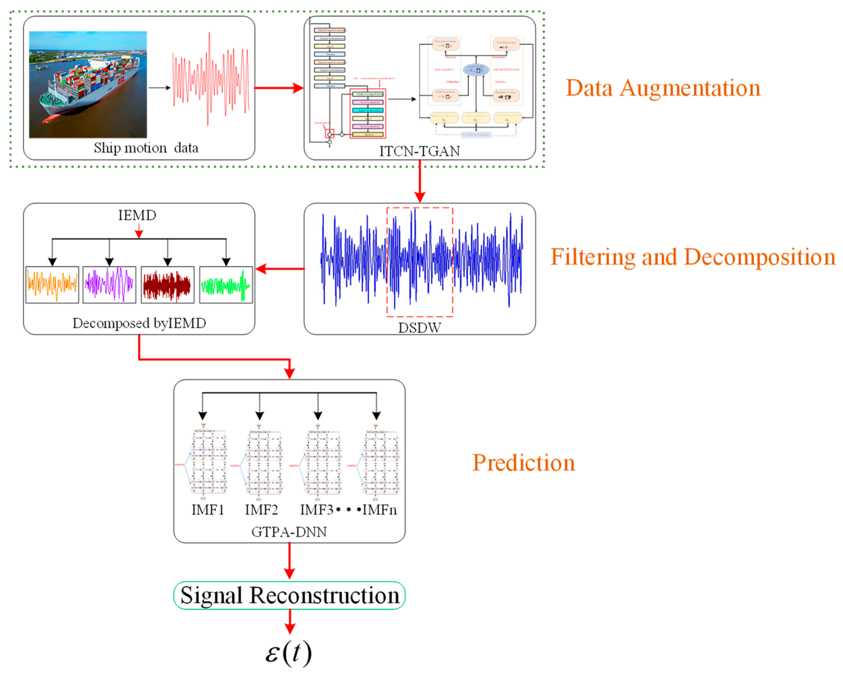
According to the Figure 13, after the ITCN-TGAN, the enhanced data are entered into the filter, in which the data with strong nonlinear characteristics are decomposed to the IMFs, which are easier to predict. IEMD directly determines the prediction difficulty of the GTPA-TNN; therefore, its validation tests take place before the validation tests of the GTPA-TNN.

In order to make the test data more suitable for the ship roll and pitch motion data under real sea conditions, the Gaussian noise is added to all the test data, the input data of IEMD and EMD are the time series in the DSDW, and their lengths are all adjusted by the DSDW, which prevents the other factors from influencing the results.

The mode mixing and endpoint effect occur in the IMFs of EMD, and the noise cannot be separated from the signal, which makes it propagate in the IMF during the decomposition process. For the above problems, the Improved Empirical Mode Decomposition algorithm is proposed, and the validation test is executed in this section.

The roll angle of KCS when $\alpha ={90}^{°}$ under the sea state of level 6 is taken as the test data, EMD is used as control, and the results of the test are offered in Figure 23 and Figure 24.

In Figure 23 and Figure 24, (a) and (b) are the IMF and the residual of the decomposition by IEMD and EMD. The test results indicate that as the decomposition progresses, the IMFs decomposed by EMD still have significant nonlinear characteristics and much noise, and its period is not obvious. The amplitude of each IMF is also much larger than that of the corresponding IMF decomposed by IEMD. The waveforms of IMF3 and IMF4 decomposed by EMD near the endpoint are quite different from those in the middle, which also indicates that the serious problem of endpoint effect exists in the IMFs of EMD. The deviation generated in the above decomposition process increases the errors of the IMFs, and the superposition of the errors causes the larger deviation in the value predicted by EMD after reconstruction.

In contrast, the decomposition results of IEMD indicate that the period of the decomposed IMFs is obvious, the nonlinear characteristic of each IMF is significantly weakened, the noise in the IMFs is obviously reduced, and the amplitude and frequency of each IMF are much lower than the corresponding IMFs decomposed by EMD, which makes the IMFs significantly easier to predict and improves the final accuracy. In addition, the waveforms near the endpoints and the middle of IMFs decomposed by IEMD are basically the same, which suggests that IEMD avoids the problem of the endpoint effect during the decomposition by the adaptive waveform extension method, which makes the IMFs able to more accurately reflect the frequency characteristic of the input signal. Compared with the IMF3–IMF6 decomposed by IEMD and EMD, the difference in nonlinear characteristics between the same level of IMFs becomes more obvious as the decomposition progresses, which indicates that the difference in decomposition efficiency between the two gradually increases and further proves that IEMD avoids the problem of noise propagation in the decomposition process. The amplitude spectrum of each IMF decomposed by IEMD and EMD is shown in Figure 25 to further compare the decomposition efficiency of IEMD and EMD.

In Figure 25, (a)–(f) are the amplitude spectrums of IMF1–IMF6 of IEMD and EMD. It can be seen from Figure 24 that the mode mixing occurs in the IMFs decomposed by EMD, especially in IMF1, IMF2, and IMF3, where four different frequency components exist at the same time, and there are also three, three, and two different frequency components in IMF4–IMF6, respectively. The mode mixing makes the IMFs not accurately reflect the frequency characteristic of the input signal, which is likely to cause the loss of important information in the original signal during the decomposition process. The amplitude spectrum of the IMFs of EMD is more scattered, which indicates that its IMFs not only have the problem of mode mixing but also have a certain amount of noise.

In contrast, there is only one frequency component in the IMFs of IEMD, and their frequency distribution is much more concentrated, which suggests that mode mixing does not occur in the IMFs. They do not interfere with each other, which can accurately characterize the frequency feature of the input sequence. On the other hand, it indicates that there is little noise in the IMFs, and the problem of noise propagation between IMFs during the decomposition process is avoided.

Finally, in order to intuitively reflect the degree of nonlinearity of the IMFs of IEMD and EMD, they are all predicted by the GTPA-TNN model. The prediction period is 60 s, the assessment index of the prediction error is the Root Mean Square Error (RMSE), and its definition is presented in Equation (46):

$${\mathrm{RMSE}}_{pre}=\sqrt{{\displaystyle \frac{1}{n}}{\displaystyle \sum _{i=1}^n{(y_i-Y_i)}^2}}$$

(46)

In Equation (41), $n$ is the number of the samples, and $Y_i$ and $y_i$ are the sample value and prediction value. The prediction results of IMF1–IMF6 are shown in Figure 26.

It can be seen from Figure 26 that the RMSE value of the IMFs of the IEMD is significantly lower than that of the IMFs of the EMD when predicted by the same model. The errors of the IMFs of EMD fluctuate in the 60 s time period, especially IMF1 and IMF2. The amplitude and frequency of their RMSE are much higher than those of other IMFs. According to Figure 23b and Figure 25, this is due to the strong nonlinear characteristic of the IMF1 and IMF2 decomposed by EMD and the serious problem of mode mixing, which significantly increases the prediction difficulty. Although the nonlinear characteristics of IMF3–IMF6 are weaker than those of IMF1–IMF3, the mode mixing and noise still exist in the IMFs, which results in the large value and amplitude of the RMSE.

For the IMFs decomposed by IEMD, the RMSE value is basically kept stable in the prediction cycle, and it is much lower than that of the corresponding IMFs decomposed by EMD. Only slight fluctuation exists at the low level, and the amplitude and frequency of the fluctuation are much lower than those of the IMFs of the same order of EMD. Compared with the IMFs of EMD, the RMSE value of the IMFs of IEMD is reduced by 46.37% at most, which further suggests that the IMFs decomposed by IEMD can accurately describe the frequency feature of the input sequence. The IMFs are independent of each other, with a high ratio of signal to noise, which verifies the validation of IEMD in avoiding the endpoint effect by the adaptive waveform extension method and filtering noise by calculating the Hausdorff distance of the input signal. In addition, the signal time-step calculation times of IEMD and EMD are 0.013 s and 0.0125 s, respectively. It can be seen that the calculation time of the two algorithms is basically the same, which can meet the need of rapid prediction.

In summary, the IEMD proposed in this study can decompose the input sequence with strong nonlinear characteristics into multiple IMFs that are easy to predict. The mode mixing, endpoint effect, and noise propagation during the decomposition all disappear due to the adaptive waveform extension method and filtering the noise. The valid information is maintained in the IMFs, which makes the IMFs able to accurately reflect the frequency characteristic of the input signal and significantly reduce the prediction difficulty of it, and the calculation period can meet the need of rapid prediction. So far, the input data are decomposed into multiple IMFs, which are easier to predict.

3.4. The Validation Test of the GTPA-TNN

According to Figure 13, the final part of the integrated model is the GTPA-TNN, which is used to predict the IMFs decomposed by IEMD. It can be seen that the DSDW, ITCN-TGAN, and IEMD of the integrated model are verified; therefore, if the validation of the TGPA-TNN can be verified, the whole integrated model can be regarded as feasible.

The validation test of the GTPA-TNN is conducted in this subsection. Considering the conventional operating sea conditions of container ships and the influence of the navigation angle, the roll and pitch angle prediction test for KCS at the sea state levels of 4 and 6 with navigation angles of 0°, 45°, and 90° is carried out. The speed of KCS is 20 Kn. The TNN (the deep time-varying residual recurrent neural network without GTPA), the LSTM, and the GRU, which are widely used in time series prediction, are taken as the contrast to prove the validation of the GTPA and time-space residual connection architecture. All the test data are decomposed into multiple IMFs by IEMD, and the settings of the four models are presented in

Table 4. The settings of the four models.

Parameter	GTPA-TNN	TNN	LSTM	GRU
Number of units in the input layer	3	3	3	3
Number of residual blocks	10	10	0	0
Number of units in the hidden layers	16.32	16.32	16.32	16.32
Number of units in the output layer	1	1	1	1
Length of the input sequence	30	30	30	30
Epoch	2500	2500	2500	2500
Optimizer	RMSprop	RMSprop	RMSprop	RMSprop
Batch size	50	50	50	50

.

In Table 4, the RMSprop is the Root Mean Square Propagation algorithm, and the input of the GTPA-TNN and TNN are both multivariate time series, which is the reason why there are three units in the input layer. The prediction periods are all 60 s. The test results of the four models for navigation angles of 0°, 45°, and 90° are presented in Figure 27, Figure 28 and Figure 29, in which (1) and (2) are the prediction curves of the roll angle and pitch angle, and (a), (b), and (c) correspond to the sea state levels of 4, 5, and 6.

The correlation coefficients of the four models are presented in Figure 27, Figure 28 and Figure 29 and are shown in

Table 5. The correlation coefficients of the four models when $\alpha =0^{°}$.

Ship Motion	LSTM			GRU			TNN			GTPA-TNN
	Lv. 4	Lv. 5	Lv. 6	Lv. 4	Lv. 5	Lv. 6	Lv. 4	Lv. 5	Lv. 6	Lv. 4	Lv. 5	Lv. 6
Roll	0.910	0.905	0.902	0.911	0.904	0.902	0.930	0.927	0.922	0.983	0.983	0.982
Pitch	0.891	0.882	0.869	0.890	0.881	0.868	0.918	0.909	0.898	0.982	0.981	0.979

,

Table 6. The correlation coefficients of the four models when $\alpha ={45}^{°}$.

Ship Motion	LSTM			GRU			TNN			GTPA-TNN
	Lv. 4	Lv. 5	Lv. 6	Lv. 4	Lv. 5	Lv. 6	Lv. 4	Lv. 5	Lv. 6	Lv. 4	Lv. 5	Lv. 6
Roll	0.902	0.891	0.881	0.901	0.889	0.880	0.924	0.917	0.906	0.981	0.979	0.977
Pitch	0.901	0.893	0.880	0.900	0.890	0.879	0.925	0.919	0.907	0.982	0.980	0.978

and

Table 7. The correlation coefficients of the four models when $\alpha ={90}^{°}$.

Ship Motion	LSTM			GRU			TNN			GTPA-TNN
	Lv. 4	Lv. 5	Lv. 6	Lv. 4	Lv. 5	Lv. 6	Lv. 4	Lv. 5	Lv. 6	Lv. 4	Lv. 5	Lv. 6
Roll	0.892	0.881	0.868	0.891	0.880	0.870	0.917	0.908	0.899	0.980	0.977	0.976
Pitch	0.909	0.904	0.901	0.911	0.903	0.902	0.931	0.925	0.921	0.984	0.983	0.982

, in which Lv. 4, Lv. 5, and Lv. 6 correspond to the sea states of levels 4, 5, and 6.

The results of the validation tests show that the GTPA-TNN can accurately predict the ship roll and pitch under the severe sea state, the prediction accuracy at each operating condition is significantly higher than that of other models, and its fluctuation amplitude is much lower than that of other models. The accuracy of the LSTM and the GRU, which are both neural networks with static structure, is far worse than that of the TNN and the GTPA-TNN. It can be seen from Table 5, Table 6 and Table 7 that there is almost no fluctuation in their correlation coefficient, which is significantly smaller than that of the TNN and the GTPA-TNN. Especially for the roll angle when $\alpha ={90}^{°}$ and the pitch angle when $\alpha =0^{°}$, the correlation coefficient of the LSTM and the GRU decreases significantly with the deterioration in sea state, which is much higher than that of the TNN and the GTPA-TNN.

It can be seen from the prediction curves shown in Figure 25, Figure 26 and Figure 27 that the accuracy fluctuation of the LSTM and the GRU in the prediction period is also much higher than that of the TNN and the GTPA-TNN. On the one hand, the wave has the most outstanding effect on the roll and pitch under the two conditions, and the nonlinear feature of the roll angle and pitch angle are significantly stronger than those of other ship motions, which makes it extremely difficult to predict; on the other hand, the LSTM and the GRU are all static models, the suitability between the architecture and the sample in the DSDW gradually decreases over time, and the rate of decline gradually increases.

In contrast, due to the time-varying structure based on the NNSOA algorithm, the TNN and GTPA-TNN can adaptively adjust the number of residual blocks according to the sample data in the DSDW to maintain the adaptability between the sample data and the model structure at an extremely high level, which verifies the validation of the time-varying architecture based on the NNSOA.

The sequential connection between hidden layers is also the reason for the low accuracy of the LSTM and the GRU. In order to avoid the gradient explosion or gradient disappearance during model training, the hidden layers are too few, which results in insufficient longitudinal depth of the model and a lack of fitting ability in predicting strong nonlinear time series. But for the TNN and the GTPA-TNN, the space–time residual connection makes their vertical depth improve significantly and avoids the above problems. Compared with the LSTM and the GRU, the correlation coefficient of the TNN and the GTPA-TNN decreases by up to 12.66% and by at least 8.87%, which suggests that spatio-temporal residual architecture improves the fitting ability for the nonlinear time series by extending the vertical depth of the neural network, and the single time-step calculation time of the TNN and the GTPA-TNN is 0.023 s and 0.025 s, respectively, which further proves that the neural network with spatio-temporal residual architecture can realize rapid prediction. In summary, the validation of the space–time residual connection architecture is preliminarily proven.

The correlation analysis of the four models is carried out to further compare the differences in their fitting ability. Considering that ship rolling has the most important influence on navigation safety, and the nonlinear characteristic of roll angle under the sea state of level 6 is far stronger than other ship motions, which make it the most difficult to predict, it can be used as the test data to maximize the difference between the performance of the models. The correlation analysis results of the four models when $\alpha$ is 0°, 45°, and 90° are presented in Figure 30. The red line is the perfect regression line.

From Figure 30, it can be seen that the correlation of the GTPA-TNN is apparently higher than that of the other three models under the sea state of level 6. According to Table 3, Table 4 and Table 5, it can be seen that, compared to other models, the correlation coefficients of the GTPA-TNN at different navigation angles are increased by at least 6.51%, 7.84%, and 8.57%, respectively. When the navigation angle is 90°, the increase in the GTPA-TNN reaches the maximum, which further proves that the GTPA-TNN can maintain high accuracy with increasing difficulty of predicting the input data, and its performance advantage will continue to increase. On the other hand, comparing the correlation coefficients of the four models when $\alpha ={90}^{°}$ under the sea states of levels 4 and 6, it can be seen that a distinguished contrast in the decrease in the correlation coefficient occurs between the four models, with the smallest decrease occurring in the GTPA-TNN, which is only 0.41%, while the LSTM, GRU, and TNN decrease by 2.69%, 2.36%, and 1.96%, respectively, which indicates that the correlation between the prediction accuracy and the nonlinear characteristic of the input sequence proves that the GTPA-TNN has strong robustness and more application value in real conditions. The error distribution of the four models under Lv. 6 is presented in Figure 31 to further compare the calculation stability of the GTPA-TNN.

According to Figure 31, it can be seen that, even for predicting ship motion under severe sea conditions, the percentage error of the GTPA-TNN is distributed between 0.8% and 2.8% and is concentrated between 1.2% and 2.5%, while the percentage errors of the LSTM, GRU, and TNN are distributed around 4~18%, 4.5~18%, and 2~11.5%, respectively, and are concentrated in 10~14.5%, 9.5~15%, and 5~10%, which suggests that the accuracy and stability of the LSTM and the GRU are extremely insufficient, and further proves that the neural network based on static structure cannot realize accurate prediction for the ship motion. In contrast, the error distribution of the TNN and the GTPA-TNN are significantly more concentrated, and the upper and lower boundaries are significantly reduced too, which further indicates that the spatio-temporal residual architecture can significantly improve the fitting capacity of the model, and the DSDW is combined with the prediction model to continuously update the sample value and adjust the number of the input data to maintain the adaptability among the sample, model structure, and sequence length.

It can be seen by comparing the percentage error of the TNN and the GTPA-TNN that the upper and lower boundaries and the length of the error distribution interval of the GTPA-TNN are all lower than those of the TNN. Even the maximum error of the GTPA-TNN is much lower than the minimum error of the TNN. On the one hand, the input sequence of the GTPA-TNN is the multivariate time series, which is composed of the ship motion data, wave height, and wave slope, which are environment factors with a high correlation with the ship motion. This makes the model mine the internal characteristics of the data from a different dimension. On the other hand, due to the GTPA, each input variable is dynamically assigned the corresponding weight, which makes the model allocate more weight to the variables with higher correlation with the output variables in the training process, and considering the global structure of the input variables, it makes the model able to accurately capture the long-term dependencies and local details between the sample data. Therefore, the length of the error distribution interval of the GTPA-TNN is basically the same when predicting the ship motion under different conditions, which indicates that the GTPA remarkably improves the accuracy and robustness of the prediction model.

In summary, the accuracy and stability of the GTPA-TNN in predicting ship motion attitudes under harsh sea states are much higher than those of the LSTM, GRU, and TNN, the performance advantage of the GTPA-TNN is more obvious with the increase in data prediction difficulty, and the prediction performance under each operating conditions is basically consistent, which proves its robustness advantage. The above results suggests that the GTPA-TNN can realize the rapid and accurate prediction of ship motion under severe sea conditions.

After verifying the validation of the DSDW, ITCN-TGAN, IEMD, and GTPA-TNN, the whole structure of the integrated model can be regarded as feasible, and an accurate and stable prediction tool for ship motion is provided.

4. Discussion

In this article, a rapid and precise integrated prediction model of ship motion under harsh sea conditions is proposed, which combines the Dynamic Sliding Data Window, the ITCN-TGAN data augmentation algorithm, the IEMD filtering algorithm, and the GTPA-TNN prediction model. The results of validation tests of the above methods indicate that the DSDW can adaptively adjust the length of the sliding data window according to the intrinsic characteristics of the sample data, which maintains the suitability between the length of the input sequence and the output variable at a high level. As a result, the calculation stability of the prediction model is indirectly improved. The ITCN-IGAN can accurately capture the time dependence between the input samples, the t-SNE distribution of the synthetic data is basically consistent with the initial data, and the prediction accuracy based on the synthetic data is also basically consistent with the original data, which proves the sufficient authenticity and validity of the data generated by the ITCN-IGAN, which can significantly reduce the sampling costs. For the IEMD, the noise in the input signal is filtered out, and the adaptive waveform extension method avoids the problems of the endpoint effect and mode mixing occurring during the training process, which significantly reduces the difficulty for predicting the ship motion. The GTPA-TNN can maintain the prediction accuracy at an extremely high level under different harsh sea conditions, and the distribution of percentage errors under each operating conditions is almost the same, which suggests its strong robustness combined with the DSDW, the ITCN-TGAN, and IEMD and ability to realize rapid and precise prediction of ship motion under severe sea conditions. Finally, the integrated model of ship motion proposed in this article will improve navigation safety and have high engineering application value. In future research, the robustness and accuracy of the prediction model will be further improved.

References

1. Song, C.Y.; Zhang, X.K.; Zhang, G.Q. Attitude prediction of ship coupled heave-pitch motions using non-linear innovation via full-scale test data. Ocean Eng. 2022, 264, 112524. [Google Scholar] [CrossRef]
2. Zheng, J.; Yan, D.W.; Yan, M.; Li, Y.; Zhao, Y.B. An unscented Kalman Filter online identification approach for a nonlinear ship motion model using a self-navigation test. Machines 2022, 10, 312. [Google Scholar] [CrossRef]
3. Mu, X.K.; Yue, G.; Zhou, N.; Chen, C.C. Occupancy grid-based AUV slam method with forward-looking sonar. J. Mar. Sci. Eng. 2022, 10, 1056. [Google Scholar] [CrossRef]
4. Jiang, H.; Duan, S.L.; Huang, L.M.; Han, Y.; Yang, H.; Ma, Q.W. Scale effects in AR model real-time ship motion prediction. Ocean Eng. 2020, 203, 107202. [Google Scholar] [CrossRef]
5. Wang, X.Y.; Tong, M.; Du, L. Multi-step prediction AR model of ship motion based on constructing and correct error. In Proceedings of the IEEE, CSAA Guidance, Navigation and Control Conference, Xiamen, China, 10–12 August 2018. [Google Scholar]
6. Kim, I.T.; Kim, S.; Paik, K.J.; Yang, J.K.; Kwon, S.Y. Free-running CFD simulations to assess a ship-manoeuvring control method with motion forecast in waves. Ocean Eng. 2023, 271, 113806. [Google Scholar] [CrossRef]
7. Liu, C.D.; Zhang, Y.F.; Gu, M.; Zhang, L.H.; Teng, Y.B.; Liu, Z.F.; Sun, Q.; Wei, N.X. Discrete Wavelet Transform-based Approach of Real-time Wave Filtering for Dynamic Positioning of Marine Vessels. Math. Probl. Eng. 2022, 5445420. [Google Scholar] [CrossRef]
8. Lu, D.H.; Zhang, Y.; Wang, J. Adaptive Delay-Free Filtering Based on IMU for Improving Ship Heave Measurement. Sensors 2023, 23, 9791. [Google Scholar] [CrossRef]
9. Wang, S.S.; Wang, L.J.; Im, N.; Zhang, W.D.; Li, X.J. Real-time parameter identification of ship maneuvering response model based on nonlinear Gaussian Filter. Ocean Eng. 2022, 247, 110471. [Google Scholar] [CrossRef]
10. Nie, Z.H.; Shen, F.; Xu, D.J.; Li, Q.H. An EMD-SVR model for short-term prediction of ship motion using mirror symmetry and SVR algorithms to eliminate EMD boundary effect. Ocean Eng. 2020, 217, 107927. [Google Scholar] [CrossRef]
11. Xu, D.X.; Yin, J.C. An enhanced hybrid scheme for ship roll prediction using support vector regression and TVF-EMD. Ocean Eng. 2024, 307, 117951. [Google Scholar] [CrossRef]
12. Li, M.W.; Xu, D.Y.; Geng, J.; Hong, W.C. A ship motion forecasting approach based on empirical mode decomposition method hybrid deep learning network and quantum butterfly optimization algorithm. Nonlinear Dyn. 2022, 107, 2447–2467. [Google Scholar] [CrossRef]
13. Qiang, H.B.; Jin, S.; Feng, X.Y.; Xue, D.P.; Zhang, L.J. Model Predictive Control of a Shipborne Hydraulic Parallel Stabilized Platform Based on Ship Motion Prediction. IEEE Access 2020, 8, 181880–181892. [Google Scholar] [CrossRef]
14. Takami, T.; Nielsen, U.D.; Jensen, J.J. Estimation of autocorrelation function and spectrum density of wave-induced responses using prolate spheroidal wave functions. J. Mar. Sci. Technol. 2020, 26, 772–791. [Google Scholar] [CrossRef]
15. Huang, Y.T.; Zhu, M.; Zheng, Z.W.; Low, K.H. Linear Velocity-Free Visual Servoing Control for Unmanned Helicopter Landing on a Ship With Visibility Constraint. IEEE Trans. Syst. Man Cybern.-Syst. 2021, 52, 2979–2993. [Google Scholar] [CrossRef]
16. Liu, Y.C.; Duan, W.Y.; Huang, L.M.; Duan, S.L.; Ma, X.W. The input vector space optimization for LSTM deep learning model in real-time prediction of ship motions. Ocean Eng. 2020, 213, 107681. [Google Scholar] [CrossRef]
17. Wang, N.; Kong, X.J.; Ren, B.Y.; Hao, L.Z.; Han, B. SeaBil: Self-attention-weighted ultrashort-term deep learning prediction of ship maneuvering motion. Ocean Eng. 2023, 287, 115890. [Google Scholar] [CrossRef]
18. Lee, D.; Lee, S.J. Motion predictive control for DPS using predicted drifted ship position based on deep learning and replay buffer. International J. Nav. Archit. Ocean Eng. 2021, 12, 768–783. [Google Scholar] [CrossRef]
19. Selimovic, D.; Hrzic, F.; Prpic-Orsic, J.; Lerga, J. Estimation of sea state parameters from ship motion responses using attention-based neural networks. Ocean Eng. 2023, 281, 114915. [Google Scholar] [CrossRef]
20. Huang, L.F.; Pena, B.; Liu, Y.C.; Anderlini, E. Machine learning in sustainable ship design and operation: A review. Ocean Eng. 2022, 266, 112907. [Google Scholar] [CrossRef]
21. Panda, J.P. Machine learning for naval architecture, ocean and marine engineering. J. Mar. Sci. Technol. 2023, 28, 1–26. [Google Scholar] [CrossRef]
22. Panda, J.P.; Warrior, H.V. Data-Driven Prediction of Complex Flow Field Over an Axisymmetric Body of Revolution Using Machine Learning. J. Offshore Mech. Arct. Eng.-Trans. Asme 2022, 144, 060903. [Google Scholar] [CrossRef]
23. Sun, Q.; Tang, Z.; Gao, J.P.; Zhang, G.C. Short-term ship motion attitude prediction based on LSTM and GPR. Appl. Ocean Res. 2022, 118, 102927. [Google Scholar] [CrossRef]
24. Zhang, T.; Zheng, X.Q.; Liu, M.X. Multiscale attention-based LSTM for ship motion prediction. Ocean Eng. 2021, 230, 109066. [Google Scholar] [CrossRef]
25. Zhou, T.; Yang, X.; Ren, H.X.; Li, C.; Han, J. The prediction of ship motion attitude in seaway based on BSO-VMD-GRU combination model. Ocean Eng. 2023, 288, 115977. [Google Scholar] [CrossRef]
26. Li, M.W.; Xu, D.Y.; Geng, J.; Hong, W.C. A hybrid approach for forecasting ship motion using CNN-GRU-AM and GCWOA. Appl. Soft Comput. 2021, 114, 108084. [Google Scholar] [CrossRef]
27. Yin, J.C.; Perakis, A.N.; Wang, N. A real-time ship roll motion prediction using wavelet transform and variable RBF network. Ocean Eng. 2018, 160, 10–19. [Google Scholar] [CrossRef]
28. Wei, Y.Y.; Chen, Z.Z.; Zhao, C.; Chen, X.; He, J.H.; Zhang, C.Y. A time-varying ensemble model for ship motion prediction based on feature selection and clustering methods. Ocean Eng. 2023, 270, 113659. [Google Scholar] [CrossRef]
Figure 1. The updated algorithm of the length of the sliding data window.
Jmse 12 02287 g001
Figure 2. The calculation process of SA.
Jmse 12 02287 g002
Figure 3. The structure of the ITCN.
Jmse 12 02287 g003
Figure 4. The operation mechanism between the components.
Jmse 12 02287 g004
Figure 5. The process of co-training.
Jmse 12 02287 g005
Figure 6. The calculation of the adaptive waveform extension method.
Jmse 12 02287 g006
Figure 7. The Global Time Attention Pattern.
Jmse 12 02287 g007
Figure 8. The structure of the inception module with residual connection.
Jmse 12 02287 g008
Figure 9. The Neural Network Structure Online Adjustment algorithm.
Jmse 12 02287 g009
Figure 10. The residual module connected by space residual connection.
Jmse 12 02287 g010
Figure 11. The structure of the Bi-TRGRU and the Bi-LSTM.
Jmse 12 02287 g011
Figure 12. The structure of the RGRU and RLSTM.
Jmse 12 02287 g012
Figure 13. Integrated prediction model.
Jmse 12 02287 g013
Figure 14. The validation of the DSDW.
Jmse 12 02287 g014
Figure 15. The error of different sliding data windows at each time step.
Jmse 12 02287 g015
Figure 16. The variation trend of the length of the DSDW with time.
Jmse 12 02287 g016
Figure 17. The t-SNE distribution of the data generated by the ITCN-TGAN on the dataset of the rolling angle when α = 90 ° under Lv. 6.
Jmse 12 02287 g017
Figure 18. The t-SNE distribution of the data generated by the GAN on the dataset of the rolling angle when α = 90 ° under Lv. 6.
Jmse 12 02287 g018
Figure 19. The t-SNE distribution of the data generated by the ITCN-TGAN on the dataset of the pitch angle when α = 0 ° under Lv. 6.
Jmse 12 02287 g019
Figure 20. The t-SNE distribution of the data generated by the GAN on the dataset of the pitch angle when α = 0 ° under Lv. 6.
Jmse 12 02287 g020
Figure 21. The prediction results from using different datasets.
Jmse 12 02287 g021
Figure 22. The error of the ITCN-TGAN and the GAN at each time step.
Jmse 12 02287 g022
Figure 23. The variation trend of the length of the DSDW with time.
Jmse 12 02287 g023
Figure 24. The residual of the validation tests of IEMD.
Jmse 12 02287 g024
Figure 25. The amplitude spectrum of each IMF in the IEMD validity tests.
Jmse 12 02287 g025
Figure 26. The error of the IMFs of IEMD and EMD.
Jmse 12 02287 g026
Figure 27. The prediction results when α = 0 ° .
Jmse 12 02287 g027
Figure 28. The prediction results when α = 45 ° .
Jmse 12 02287 g028
Figure 29. The prediction results when α = 90 ° .
Jmse 12 02287 g029
Figure 30. Correlation analysis of the four models at sea level 6.
Jmse 12 02287 g030
Figure 31. The error distribution of the four models at Lv. 6.
Jmse 12 02287 g031