A De-Nesting Hybrid Reliability Analysis Method and Its Application in Marine Structure

Abstract

In recent years, marine structures have been widely used in the world, making significant contributions to the utilization of marine resources. In the design of marine structures, there is a hybrid reliability problem arising from aleatory uncertainty and epistemic uncertainty. In many cases, epistemic uncertainty is estimated by interval parameters. Traditional methods for hybrid reliability analysis usually require a nested optimization framework, which will lead to too many calls to the limit state function (LSF) and result in poor computational efficiency. In response to this problem, this paper proposes a de-nesting hybrid reliability analysis method creatively. Firstly, it uses the p-box model to describe the epistemic uncertainty variables, and then the linear approximation (LA) model and the two-point adaptive nonlinear approximation (TANA) model are combined to approximate the upper and lower bounds of LSF with epistemic uncertainty. Based on the first-order reliability method (FORM), an iterative operation is used to obtain the interval of the non-probability hybrid reliability index. The traditional nested optimization structure is effectively eliminated by the above approximation method, which efficiently reduces the times of LSF calls and increases the calculation speed while preserving sufficient accuracy. Finally, one numerical example and two engineering examples are provided to show the greater effectiveness of this method than the traditional nested optimization method.

1. Introduction

In order to meet the needs of safety and economy of marine structures, uncertainty as a key factor in the design and manufacture of marine structures has been widely studied. Uncertainty in marine engineering includes aleatory uncertainty and epistemic uncertainty [1,2]. Aleatory uncertainty is caused by the inherent randomness of relevant variables in structures and ocean environments, which is usually described by an accurate probability distribution. Epistemic uncertainty is caused by the lack of sufficient knowledge or incomplete information about the variables, which can be described in the form of intervals and probabilistic methods [3].

In the past decades, aleatory uncertainty associated with marine structures has been a subject of extensive research. The traditional reliability assessment method is to use the FORM or the second-order reliability method (SORM) to calculate the structural reliability index after quantifying the uncertainty of random variables using probabilistic models [4], and the continuous development of reliability theory provides new tools for the reliability analysis of marine structures. Homaei and Najafzadeh [5] combined the artificial intelligence method and Monte Carlo sampling (MSC) to analyze the reliability of pile group scour depth being less than a limit value under regular waves. Aghatise Okoro et al. [6] used the polynomial chaos expansion (PCE) and Kriging method to construct a metamodel of the limit state function and reduced the computational time by the MSC method. Ming Cai Xu et al. [7] used the model correction factor method (MCFM) to constantly revise the results at the design points in the FORM iteration process to ensure that the results of the simplified model were close to the real model. The above research focuses on how to construct a surrogate model that is closer to the real model. However, their random variable distributions are usually based on empirical assumptions.

In fact, obtaining the accurate distribution of random variables requires a large number of sample data, which is difficult to achieve in practical engineering applications. In addition, it is often difficult to eliminate the uncertainty caused by structural manufacturing, installation errors and parameter measurement errors. To facilitate calculations, the aforementioned epistemic uncertainties are transformed into deterministic factors in many cases, leading to errors in the reliability assessment of marine structures. Debiao Meng et al. [8] analyzed the fatigue of offshore wind turbine structures and showed that a reliability assessment framework that considers both aleatory and epistemic uncertainties is more accurate and conservative. Therefore, it is necessary to incorporate the analysis method of epistemic uncertainty into the reliability assessment of marine structures.

In 1989, Ben-Haim and Elishakoff [9] proposed the idea of a non-probabilistic reliability model. Based on their study and the traditional probability theory, researchers began to propose a variety of non-probability models to describe the epistemic uncertain variables affecting structural reliability, such as interval theory [10,11], convex set theory [12,13], evidence theory [14,15] and p-box theory [16,17,18], etc. In many non-probabilistic models, it is simple and feasible to describe epistemic uncertain variables by using the interval model or the convex set model. The interval model and the convex set model envelope sample data points to obtain a hypercube or a super ellipsoid, which is the description of the epistemic uncertain variable. However, the interval model or the convex model only uses the edge data of the sample data, but does not make full use of information such as the dense distribution of internal data. This may lead to an overestimation of the epistemic uncertain variable and furthermore an excessively large interval of analysis results. The final result provides no effective guidance for solving practical engineering problems. Moreover, technicians can effectively estimate the distribution of epistemic uncertainty variables in some cases with their engineering experience and the analytical results of similar structures. However, this reference information cannot be effectively utilized with the interval model or the convex set model due to their theoretical limitations. As a new type of non-probability model theory, p-box theory describes the epistemic uncertain variable through the upper and lower probability boxes of the cumulative distribution function (CDF). Regardless of whether the distribution form is unknown or known, epistemic uncertain variables can be described by the p-box model [16]. In addition, p-box theory is compatible with other common non-probability theories. That is, other non-probability models can be transformed to the p-box model to some extent. Therefore, p-box theory can be used to establish a non-probability model with broader applicability for structural reliability analysis with epistemic uncertain variables. Research on the p-box model is burgeoning. Zhang et al. [19] obtained the statistical moments and the CDF of a response function with a non-parametric p-box variable based on the cumulative distribution function discretization (CDFD) method. Li and Jiang [20] combined the stochastic processes with p-box theory to propose a p-box-based imprecise stochastic process model, which is used for uncertainty analysis of structures under uncertain dynamic excitations or time-variant factors. Xiao et al. [21] proposed a collaborative interval quasi-Monte Carlo method (CIMCM) to deal with the reliability model with multiple types of epistemic uncertainty unified by p-boxes variables, combining Rosen’s gradient projection method (RGPM) and collaborative optimization strategy, making the simulation convergence faster.

After the establishment of the non-probabilistic hybrid reliability model of the structure by using the traditional probabilistic model and the non-probability model, a hybrid structure reliability analysis is needed. At present, most of the literature needs to establish a two-layer nested optimization model [22,23,24]. The outer layer is the process of traditional structural reliability optimization, and the inner layer is the optimization model of the limit value of the LSF with the epistemic uncertain variables as the optimization vector. Due to the existence of the inner optimization structure, this nested optimization structure requires a large number of calls to the LSF, resulting in an inefficient calculation.

Referencing the FORM, this paper deals with the case of epistemic uncertainty variables with small uncertainty and combines the linear approximation (LA) model and the two-point adaptive nonlinear approximation (TANA) model to approximate the upper and lower limits of the response of the LSF. Consequently, a de-nesting analysis method of the non-probabilistic hybrid reliability index based on an approximation model is proposed. In this paper, the U space (standard normal distribution space) is converted back to original space of the LSF, and the boundary of the corresponding p-box variable is obtained. The approximation method eliminates the inner layer of the original nested optimization structure. The outer layer of the original nested optimization structure of the hybrid reliability analysis is transformed into a traditional optimization problem, with the constraint that the inner layer is expressed as an approximate formulation developed at the design point. The speed of non-probabilistic hybrid reliability analysis of structures will be effectively improved because of the elimination of nested structures. Finally, the proposed reliability assessment method is applied to a numerical example and two common marine structures to verify its effectiveness and superiority.

2. Non-Probabilistic Hybrid Structural Reliability

2.1. P-Box Theory

In p-box theory, the p-box model is a probability box enveloped by the upper and lower limits of the CDF, and a precise distribution form of variable distribution is difficult to obtain. When the distribution type of the variable is known, a more accurate p-box model can be obtained by estimating the interval of the distribution parameters of the distribution type. If the distribution type of the variable cannot be obtained, the Chebyshev inequality can be used to rigorously derive the upper and lower limits of the CDF of the variable, using information such as the origin moment of the sample data.

If the variable y is described by the p-box model, it can be expressed as Equation (1) and Figure 1.

$$\underset{¯}{F_Y}(y)\le F_Y(y)\le \overline{F_Y}(y)$$

(1)

The p-box model can be called a parametric p-box model when the distribution type of the epistemic uncertain variable is known and the distribution parameter is an estimation interval. When only the upper and lower limits of the CDF of the uncertain variable are known, the p-box model can be called a free p-box model.

The acquisition method of the free p-box model is generally Chebyshev’s inequality, and the upper and lower limits of the CDF of the variable Y can be expressed as Equation (2a,b).

$$\underset{¯}{F_Y}(y)=\left\{\begin{array}{c}0, y<\mu +\sigma \hfill \\ 1-{\displaystyle \frac{{\sigma }^2}{{(y-\mu )}^2}}, y\ge \mu +\sigma \end{array}\right.$$

(2a)

as well as

$$\overline{F_Y}(y)=\left\{\begin{array}{c}{\displaystyle \frac{{\sigma }^2}{{(y-\mu )}^2}}, y<\mu -\sigma \\ 1, y\ge \mu -\sigma \hfill \end{array}\right.$$

(2b)

where $\overline{F_Y}(y)$ and $\underset{¯}{F_Y}(y)$ are the upper and lower limits of the CDF of the variable y, respectively, and $\mu$ and $\sigma$ are the mean and standard deviation of the epistemic uncertain variable $y$ in the sample data.

For the parametric p-box model, the CDF of the variable y can be expressed as Equation (3).

$$F_Y(y)=F_Y(y|\tau ),s.t. \tau \in [\underset{\_}{\tau },\overline{\tau }]$$

(3)

where $\tau$ is the distribution parameter of the distribution type that the variable y follows. Due to the small amount of sample data and other possible reasons, this parameter is generally impossible to obtain accurately, but it can be estimated by the interval $[\underset{\_}{\tau },\overline{\tau }]$.

2.2. Analytical Method

In the structural reliability analysis process, if the variable affecting the structural reliability contains n random variables $X=(x_1,x_2,\cdots ,x_n)$ (the exact CDF is known) and $m$ p-box variables $Y=(y_1,y_2,\cdots ,y_m)$ (the exact CDF is unknown), the LSF $g(X,Y)$ of the structure can be obtained.

$$\left\{\begin{array}{c}g(X,Y)<0,\cdots Structural\cdot failure\\ g(X,Y)=0,\cdots \cdots \cdots Limit\cdot state\\ g(X,Y)>0,\cdots Structural\cdot safety\end{array}\right.$$

(4)

To use FORM for structural reliability analysis, it is necessary to convert the LSF from the original space to the standard normal space (U space). The LSF in U space can be obtained by probability conversion, i.e., $\mathrm{G}(U_X,U_Y)=g(X,Y)$ ($U_X$, $U_Y$) are independent standard normal distribution variables.

The independent variables $X$ and $Y$ after converting from the original space to the U space are given by

$$\left\{\begin{array}{l}{U}_X={\mathsf{\Phi }}^{-1}\left(F_X\left(X\right)\right)\\ U_Y={\mathsf{\Phi }}^{-1}\left(F_Y\left(Y\right)\right)\end{array}\right.$$

(5)

where $F_X\left(X\right)$ is the CDFs of the random variables $X$, $F_Y\left(Y\right)$ is the CDFs of the p-box variables $Y$ and ${\mathsf{\Phi }}^{-1}$ is the inverse of the standard normal distribution.

According to Equation (5), there is,

$$\left\{\begin{array}{l}X=F_X^{-1}(\mathsf{\Phi }(U_X))\\ Y=F_Y^{-1}(\mathsf{\Phi }(U_Y))\in [Y^L,Y^R]=[{\overline{F_Y}}^{-1}(\mathsf{\Phi }(U_Y)),{\underset{¯}{F_Y}}^{-1}(\mathsf{\Phi }(U_Y))]\end{array}\right.$$

(6)

where $F_X^{-1}$ is the inverse functions of the CDFs of the random variables $X$, and $F_Y^{-1}$ is the inverse function of the CDFs of the p-box variables $Y$. ${\overline{F_Y}}^{-1}$ and ${\underset{¯}{F_Y}}^{-1}$ are, respectively, the inverse functions of the upper and lower limits of the CDFs of the p-box variables $Y$, and $Y^L$ and $Y^R$ are the lower and upper value limits of the p-box variables $Y$.

Further, the LSF for the structure can be expressed as Equation (7).

$$\left\{\begin{array}{l}g(X,Y)=G(U_X,U_Y)=G\left({\mathsf{\Phi }}^{-1}(F_X(X)),{\mathsf{\Phi }}^{-1}(F_Y(Y))\right)\\ \mathrm{G}(U_X,U_Y)=g(X,Y)=g\left(F_X^{-1}(f(U_X)),F_Y^{-1}(f(U_Y))\right)\end{array}\right.$$

(7)

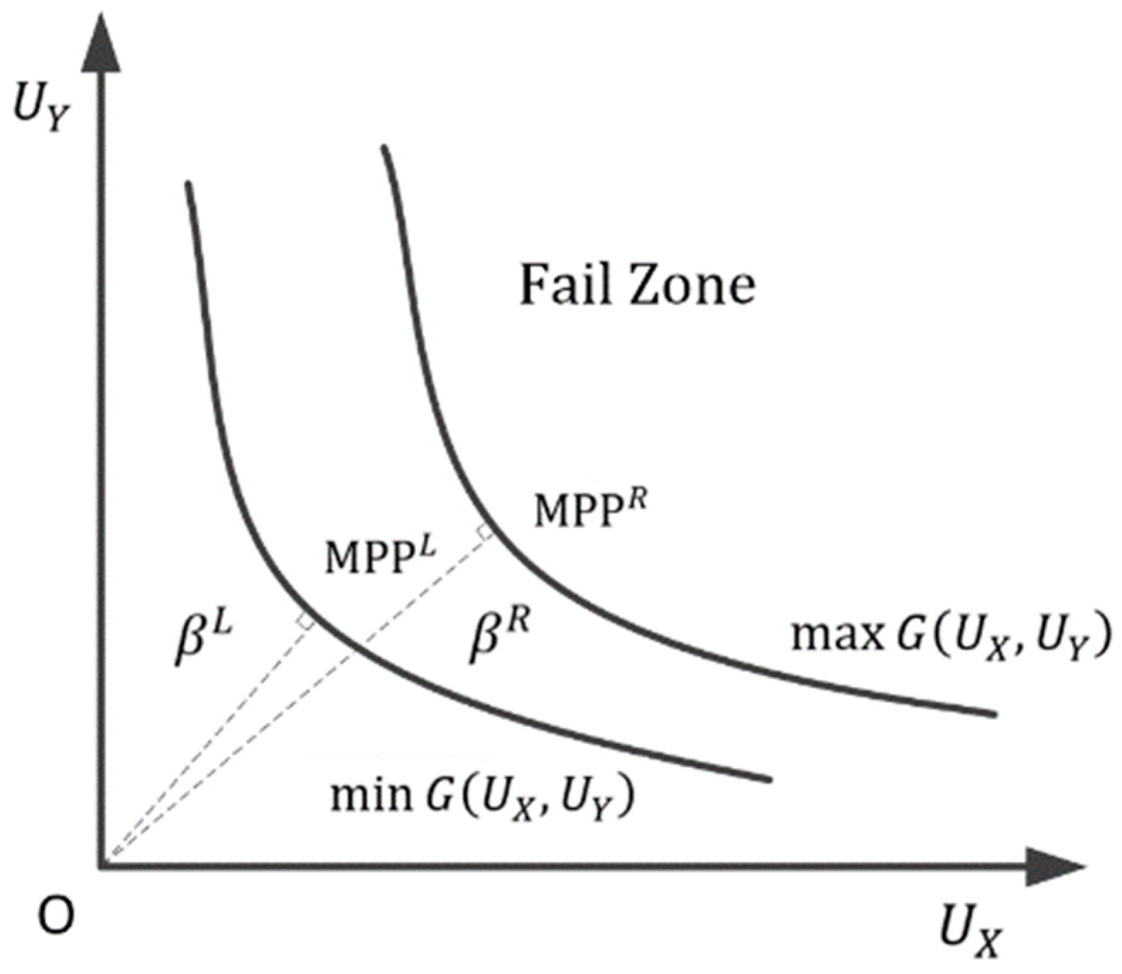
Since the variables $Y\in [Y^L,Y^R]$ are p-box variables, the structural LSF can be written as Equation (8), and Figure 2 shows the surfaces of the non-probability hybrid LSF in the U space.

$$\mathrm{G}(U_X,U_Y)=g(X,Y)\in [g^L,g^R]$$

(8)

where $g^L={\min }_{Y}g(X,Y)={\min }_{\cdot }G(U_X,U_Y)$, and $g^R=\underset{Y}{\max }g(X,Y)=\underset{\mathrm{G}}{\max }(U_X,U_Y)$.

In Figure 2, MMP^L and MMP^R represent the maximum possible failure points (MPPs) of the lower LSF $g^L$ and upper LSF $g^R$, respectively. ${\beta }^L$ and ${\beta }^R$ are the upper and lower limits of the reliability index $\beta$. According to the FORM, the structural reliability index $\beta$ can be obtained, that is,

$$\left\{\begin{array}{l}\beta ={\min }_{U_X,U_Y}\sqrt{U_X^T{U}_X+U_Y^T{U}_Y}\\ s.t.\mathrm{G}(U_X,U_Y)=g(X,Y)=0\end{array}\right.$$

(9)

It can be known from Equations (8) and (9) that the non-probability hybrid reliability index $\beta$ can be written as $\beta \in [{\beta }^L,{\beta }^R]$. Further, two nested optimization functions related to the upper and lower limits of the reliability index $\beta$ can be obtained, as shown in Equation (10a,b).

$$\left\{\begin{array}{l}{\beta }^L=\underset{U_X,U_Y}{\min }\sqrt{U_X^T{U}_X+U_Y^T{U}_Y}\hfill \\ s.t. G^L=g^L=\underset{Y}{\min }g(X,Y)=0\hfill \end{array}\right.$$

(10a)

and

$$\left\{\begin{array}{l}{\beta }^R=\underset{U_X,U_Y}{\min }\sqrt{U_X^T{U}_X+U_Y^T{U}_Y}\hfill \\ s.t. G^R=g^R=\underset{Y}{\max }g(X,Y)=0\hfill \end{array}\right.$$

(10b)

At the same time, it is necessary to discern the sign of the $\beta$. This requires obtaining the sign of the LSF at the origin of the standard normal space. According to Equation (11), the correct sign of $\beta$ can be determined.

$${\beta }^{R(L)}=\mathrm{sgn}(G^{R(L)}(0,0)){\beta }^{R(L)}=\mathrm{sgn}(g^{R(L)}({\mu }_X,{\mu }_Y)){\beta }^{R(L)}$$

(11)

In Equation (11), sgn represents a function that indicates the sign of $G^{R(L)}(0,0)$.

It can be known from Equation (10a,b) that the problem of hybrid structural reliability analysis with the p-box variables is a nested optimization problem. The inner layer is the process of solving the extremum of the LSF. For the above nested optimization problem, the computational workload of the traditional optimization algorithm is too heavy. In order to improve the calculation speed, the idea of an approximation model is used to approximate the upper and lower limits of the LSF. As such, the double-layer nested optimization structure is eliminated, the original optimization problem is transformed into a general optimization problem and finally a non-probabilistic hybrid reliability analysis method with p-box variables is constructed.

3. Approximation Model

In order to approximate the limit value of the LSF, it is necessary to use the approximation model. In this paper, the single-point approximation model and the two-point adaptive nonlinear approximation model are combined to approximate the LSF.

3.1. Single-Point Approximation Model

Based on the function value and gradient information at a single point, a single-point approximation model is established at the design point according to the first-order Taylor series. When using the traditional method optimization, since the search direction always needs to calculate the function value and the first derivative value in the optimization process, there is no need to add the calculation amount when constructing the single-point approximation model. There are a variety of single-point approximation models based on first-order Taylor expansion, including the linear approximation (LA) model, the reciprocal approximation model [25] and the conservative approximation model [26]. The single-point linear approximation model can be expressed as Equation (12).

$$g(X)=g(X_k)+\sum _i^n{\displaystyle \frac{\partial g(X_k)}{\partial x_i}}(x_i-x_{i,k})$$

(12)

3.2. Two-Point Adaptive Nonlinear Approximation (TANA) Model

When using the single-point approximation model based on the first-order Taylor series, as the iteration proceeds, a new approximate model needs to be reconstructed at the new design point. The analysis information of the previous iteration step will be discarded and will not be used to improve the subsequent approximation model, resulting in relatively low fitting accuracy.

The two-point adaptive nonlinear approximation model is based on not only the information of the current design point, but also the information of the previous iteration point, and the nonlinear characteristic of the TANA model is automatically adjustable by the function value and the gradient values of the known point. Therefore, the TANA model is an adaptive approximation model whose simulation accuracy is higher than the single-point approximation model. The intermediate variable $z_i$ of the TANA model can be expressed as [27,28],

$$z_i=x_i^r,i=1,2,\cdots ,n$$

(13)

For any variable $x_i$, the nonlinear index is equal to r.

When establishing a TANA model, the function values of the two points and the gradient values of the design points are necessary. First, the intermediate variable $z_i$ is used to represent the first-order Taylor expansion of the design point, and the variable $x_i$ is used in place of $z_i$ in the extended expression. Typically, one of the two points is selected as the new design point and the other point is selected as the design point of the previous iteration. Its mathematical expression is

$$g(X)=g(X_k)+{\displaystyle \frac{1}{r}}\sum _i^n{x}_{i,k}^{1-r}{\displaystyle \frac{\partial g(X_k)}{\partial x_i}}(x_i^r-x_{i,k}^r)$$

(14)

where $X_k$ denotes the design point of the kth iteration and r denotes the nonlinear index. The nonlinear index will change during each iteration. The nonlinear index is determined by matching the function value at the previous design point $X_{k-1}$. That is, the difference between the approximation value and the exact value of $g\left(X_{k-1}\right)$ is zero.

$$g(X_{k-1})-\left(g(X_k)+{\displaystyle \frac{1}{r}}\sum _i^n{x}_{i,k}^{1-r}{\displaystyle \frac{\partial g(X_k)}{\partial x_i}}(x_{i,k-1}^r-x_{i,k}^r)\right)=0$$

(15)

In order to reduce the iterative calculation of the high-order polynomial approximation model, r can be limited as $r\in [-5,5]$. This paper gives an idea of a solution. By constructing an optimization model, the nonlinear index r is obtained.

$$\left\{\begin{array}{l}find r\\ \underset{r}{\min }\left|g(X_{k-1})-\left(g(X_k)+{\displaystyle \frac{1}{r}\sum _i^n}{x}_{i,k}^{1-r}{\displaystyle \frac{\partial g(X_k)}{\partial x_i}}(x_{i,k-1}^r-x_{i,k}^r)\right)\right|\\ s.t.-5\le r\le 5\end{array}\right.$$

(16)

It can be understood from Equations (11) and (13) that the LA model is a special case of the TANA model. When the nonlinear index $r=1$, the TANA model is an LA model. The single-point approximation model is constructed according to the function value and the first-order derivative values at the design point, whereas in the TANA mode, the function value of another point is used to adjust the nonlinear index r such that the approximation value is equal to the exact function value. Therefore, the approximation accuracy of TANA is higher than the single-point approximation model.

Figure 3 shows a comparison of the approximation of the function using the LA model and the TANA model at design point x = 1. Another point selected by the TANA model is $x_2=1.3$, and the nonlinear index is calculated as $r=-1.073$. It can be seen that the LA model can only approximate the original function with linear precision, and its approximation accuracy for strong nonlinear functions is poor. The approximation accuracy of the TANA model is significantly higher than the LA model, and there is no need to calculate the high-order derivative.

4. De-Nesting Analysis Method

4.1. De-Nesting Theory

For the non-probabilistic hybrid structural reliability model, the LSF is $g\left(X,Y\right)$, and the method for calculating the structural reliability index is shown in Equation (10a,b). For $g\left(X,Y\right)$, since all of the epistemic uncertainty variables in practical engineering applications are of small uncertainty and the LA model is suitable for expanding the LSF in such scenarios, a satisfactory precision can be achieved. It is used to expand $g\left(X,Y\right)$ at $\left(X,Y^C\right)$, and its mathematical expression is

$$g(X,Y)\approx g(X,Y^c)+\sum _{j=1}^m{\displaystyle \frac{\partial g(X,Y^c)}{\partial y_j}}(y_j-y_j^c)$$

(17)

In Equation (17), there is $Y^c=(Y^L+Y^R)/2$ and $y_j^c=\left(y_j^L+y_j^R\right)/2$.

Using the TANA model to approximate $g\left(X,Y^C\right)$ at point $g\left(X_s,Y_s^C\right)$ to obtain Equation (18a), it is not difficult to substitute Equation (17) into Equation (18a), which combines the LA model and the TANA model to approximate the LSF, as shown in Equation (18b).

$$\left\{\begin{array}{l}g(X,Y^c)=g(X_s,Y_s^c)+R_n(X,r)+R_m(Y,r)\\ R_n(X,r)={\displaystyle \frac{1}{r}\sum _i^n}{x}_{i,s}^{1-r}{\displaystyle \frac{\partial g(X_s,Y_s^c)}{\partial x_i}}(x_i^r-x_{i,s}^r)\\ R_m(Y^c,r)={\displaystyle \frac{1}{r}\sum _j^m}{(y_{j,s}^c)}^{1-r}{\displaystyle \frac{\partial g(X_s,Y_s^c)}{\partial {\gamma }_i^c}}({(y_j^c)}^r-{(y_{j,s}^c)}^r)\end{array}\right.$$

(18a)

where s = 1, 2, 3 …

$$g(X,Y)\approx g(X_s,Y_s^c)+R_n(X,r)+R_m(Y,r)+\sum _{j=1}^m{\displaystyle \frac{\partial g(X,Y^c)}{\partial y_j}}(y_j-y_j^c)$$

(18b)

Substitute Equation (18b) into Equation (10a,b), and two de-nesting optimization functions related to the upper and lower limits of the reliability index can be obtained; for any nonlinear index $r=r_s$, there is

$$\left\{\begin{array}{l}\beta =\underset{U_X,U_Y}{\min }\sqrt{U_X^T{U}_X+U_Y^T{U}_Y}\\ s.t.g^L\approx \underset{Y}{\min }\left(g(X_s,Y_s^c)+R_n(X,r)+R_m(Y^c,r)+{\displaystyle \sum _{j=1}^m\frac{\partial g(X,Y^c)}{\partial y_j}}(y_j-y_j^c)\right)=0\end{array}\right.$$

(19a)

$$\left\{\begin{array}{l}\beta =\underset{U_X,U_Y}{\min }\sqrt{U_X^T{U}_X+U_Y^T{U}_Y}\\ s.t.g^R\approx \underset{Y}{\max }\left(g(X_s,Y_s^c)+R_n(X,r)+R_m(Y^c,r)+{\displaystyle \sum _{j=1}^m\frac{\partial g(X,Y^c)}{\partial y_j}}(y_j-y_j^c)\right)=0\end{array}\right.$$

(19b)

In Equation (19a,b), $X_S$ and $Y_S$ are obtained by probability conversion at the design expansion point $\left(U_{X,S},U_{Y,S}\right)$ after sth iterations. In other words, there is

$$X_s=F_X^{-1}(\mathsf{\Phi }(U_{X,s})),Y_s\in [{\overline{F_Y}}^{-1}(\mathsf{\Phi }(U_{Y,s})),{\underset{¯}{F_Y}}^{-1}(\mathsf{\Phi }(U_{Y,s}))]$$

(20)

$Y_S^C$ is the median point of the p-box variable Y after the sth iteration. There is

$$Y_s^c=({\overline{F_Y}}^{-1}(\mathsf{\Phi }(U_{Y,s})))+{\underset{¯}{F_Y}}^{-1}(\mathsf{\Phi }(U_{Y,s}))/2$$

(21)

The nonlinear index r can be solved with Equation (16).

$$\left\{\begin{array}{l}find r\\ \underset{r}{\min }|g(X_{s-1},Y_{s-1}^c)-(g(X_s,Y_s^c)+R_n(X_{s-1},r)+R_m(Y_{s-1}^c,r))|\\ s.t.-5\le r\le 5\end{array}\right.$$

(22)

According to interval theory, the $g^L$ can be approximated using Equation (10a), which is

$$\begin{array}{ll}{g}^L& \approx \underset{Y}{\min }(g(X_s,Y_s^c)+R_n(X,r)+R_m(Y^c,r)+{\displaystyle \sum _{j=1}^m\frac{\partial g(X,Y^c)}{\partial y_j}}(y_j-y_j^c))\\ & =g\left(X_S,Y_S^X\right)+R_n(X,r)+R_m(Y^c,r)-{\displaystyle \sum _{j=1}^m\left|\frac{\partial g(X,Y^c)}{\partial y_j}\right|}\left({\displaystyle \frac{y_j^R-y_j^L}{2}}\right)\end{array}$$

(23a)

Similarly, $g^R$ should be

$$\begin{array}{ll}{g}^R& \approx \underset{Y}{\max }(g(X_s,Y_s^c)+R_n(X,r)+R_m(Y^c,r)+{\displaystyle \sum _{j=1}^m\frac{\partial g(X,Y^c)}{\partial y_j}}(y_j-y_j^c))\\ & =g\left(X_S,Y_S^X\right)+R_n(X,r)+R_m(Y^c,r)+{\displaystyle \sum _{j=1}^m\left|\frac{\partial g(X,Y^c)}{\partial y_j}\right|}\left({\displaystyle \frac{y_j^R-y_j^L}{2}}\right)\end{array}$$

(23b)

In the case where the form of the LSF is unknown or its first-order partial derivatives are difficult to obtain, the finite difference method can be used to address this problem.

$$\left\{\begin{array}{l}{\displaystyle \frac{\partial g(X_s,Y_s^c)}{\partial x_i}}={\displaystyle \frac{g(X_s+\mathsf{\Delta }{x}_i,Y_s^c)-g(X_s,Y_s^c)}{{‖\mathsf{\Delta }{x}_i‖}_2}}\\ {\displaystyle \frac{\partial g(X_s,Y_s^c)}{\partial y_j^c}}={\displaystyle \frac{g\left(X_s,Y_s^c+\mathsf{\Delta }{y}_j^c\right)-g(X_s,Y_s^c)}{{‖\mathsf{\Delta }{y}_j^c‖}_2}}\\ {\displaystyle \frac{\partial g(X,Y^c)}{\partial y_j}}={\displaystyle \frac{g\left(X,Y^c+\mathsf{\Delta }{y}_j\right)-g(X,Y^c)}{\mathsf{\Delta }{y}_{j2}}}\end{array}\right.$$

(24)

where $\mathsf{\Delta }{x}_i=(0,0,\cdots ,{\mathsf{\Delta }}_i,\cdots ,0)$ and $\mathsf{\Delta }{y}_j^c=\mathsf{\Delta }{y}_j=\left(0,0,\cdots ,{\mathsf{\Delta }}_j,\cdots ,0\right)$. ${\Delta }_i$ and ${\Delta }_j$ are constants that are small enough but not zero. ${‖*‖}_2$ expresses two-norm.

After going through the above process, for the double-layer nested optimization structure, the inner and outer optimization processes of the extreme value of LSF can be replaced with the approximation function, therefore eliminating the double-layer nested optimization structure and improving the calculation speed effectively. For the outer optimization problem, the TANA model is used to effectively avoid the problem that the convergence speed depends on the degree of approximation between the linearized LSF and the original nonlinear LSF. For each construction of the outer layer approximation model, $\left(n+m+1\right)$ times of solving the value of original LSF are needed at most. After the approximation model is constructed, for each time the extreme value of the approximation model is called, this process can be simplified to no more than $\left(m+1\right)$ times of original LSF value solution (one time of function value calculation at the median point and m calls of function value due to the operation of the first-order partial derivative).

When using the present non-probabilistic hybrid reliability analysis methods, both the outer optimization process and the inner optimization processes require a large number of calls to the original LSF in order to obtain the limit of the LSF response. Compared with traditional nested analysis methods, the method proposed by this paper maintains the calculation accuracy and effectively reduces the number of calls to the LSF, which saves computing resources and increases computing speed.

4.2. De-Nesting Analysis Process

After using the LA model and the TANA model to approximate the LSF and obtain the limit value of the function response according to interval theory, the FORM can be used to obtain the structural reliability index $\beta$. According to References [25,29], the iterative equation of FORM can be expressed as

$$U_{k+1}={\displaystyle \frac{{\nabla }^{T}G(U_k)U_k-G(U_k)}{{\nabla }^{T}G(U_k){\alpha }_k}}{\alpha }_k$$

(25)

where $a_k$ is the negative unit normal vector at point $U_k$. According to the HL-RF method, $a_k$ can be expressed as the following equation.

$${\alpha }_k=-{\displaystyle \frac{\nabla G(U_k)}{\parallel \nabla G(U_k)\parallel }}$$

(26)

Due to the use of TANA and LA models, there is a different $r_S$ in each approximation of the LSF. For any nonlinear index $r=r_S$, according to Equation (23a,b), the approximation expression of the upper and lower limits of the LSF can be known, that is, $G^R=g^R$ and $G^L=g^L$. The MMP can be calculated in combination with Equation (28). There are

$$U_{k+1}^{R(L)}={\displaystyle \frac{{\nabla }^T{G}^{R(L)}(U_k^{R(L)})U_k^{R(L)}-G^{R(L)}(U_k^{R(L)})}{{\nabla }^T{G}^{R(L)}(U_k^{R(L)}){\alpha }_k^{R(L)}}}{\alpha }_k^{R(L)}$$

(27)

$${\alpha }_k^{R(L)}=-{\displaystyle \frac{\nabla G^{R(L)}(U_k^{R(L)})}{\nabla G^{R(L)}(U_k^{R(L)})}}$$

(28)

where $U_k^{R(L)}=\left(U_{X,k}^{R(L)},U_{Y,k}^{R(L)}\right)$. Similarly, the finite difference method can be used to obtain $\nabla G^{R(L)}=\left(\nabla G_1^{R(L)},\nabla G_2^{R(L)},\cdots \nabla G_p^{R(L)},\cdots ,\nabla G_{m+n}^{R(L)}\right)$

$$\nabla {\mathrm{G}}_p^{R(L)}(U_{k,p}^{R(L)})={\displaystyle \frac{G^{R(L)}(U_k^{R(L)}+\mathsf{\Delta }{U}_{k,p}^{R(L)})-G^{R(L)}(U_k^{R(L)})}{{\mathsf{\Delta }}_p}}$$

(29)

where $\mathsf{\Delta }{U}_{k,p}^{R(L)}=\left(0,0,\cdots ,{\mathsf{\Delta }}_p,\cdots ,0\right)$ and ${\mathsf{\Delta }}_p$ is small enough but not zero.

For any nonlinear exponent $r=r_S$, the iterative convergence condition (1) can be set to

$$\left\{\begin{array}{l}\parallel U_{k+1}^{R(L)}-U_k^{R(L)}{\parallel }_{ 2}<\delta \\ {\beta }_{k+1,s}^{R(L)}-{\beta }_{k,s}^{R(L)}<\epsilon \end{array}\right.$$

(30)

${\beta }_{k,s}^{R(L)}$ is expressed as the reliability index calculated by the kth iteration when the nonlinear index $r=r_S$. When the iteration meets the convergence condition (1), there should be ${\beta }_s^{R(L)}={\beta }_{s,k}^{R(L)}$. At the same time, $U_s^{R(L)}=U_k^{R(L)}$ is used as the design expansion point to update the nonlinear index $r_s$ of the approximation model for the next iteration. The convergence condition (2) of the overall iterative algorithm can be set to

$${\beta }_s^{R(L)}-{\beta }_{s-1}^{R(L)}<\epsilon$$

(31)

The detailed process of the de-nesting analysis method is as follows, and the flow chart is as illustrated in Figure 4.

• Step 1: Initialize parameters (1); let $S=1$ record the number of iterations and provide an expansion point $U_S^{R\left(L\right)}$ and nonlinear index $r_S$ to provide the basis for calculation for the next step. In general, $U_1^{R\left(L\right)}=0$ and $r_S=1$, that is, linear expansion at the mean point of the variables.
• Step 2: Variable conversion. Convert the vector $U_S^{R\left(L\right)}$ of the standard normal space back to the original space of the LSF to obtain $\left(X_S,X_S^C\right)$.
• Step 3: At any point $\left(X,Y\right)$, using the LA model, the LSF approximation is expressed as an approximation expression for the p-box variables, i.e., Equation (17).
• Step 4: According to the nonlinear index $r_S$, a TANA model for $g\left(X,Y^C\right)$ is established at the point $\left(X_S,X_S^C\right)$, i.e., Equation (18).
• Step 5: Combine the LA model in the third step with the TANA model in the fourth step to approximate the extremum of the response of the LSF $g\left(X,Y\right)$ to any point $\left(X,Y\right)$.
• Step 6: Initialize parameters (2), $k=0,U_k^{R(L)}=U_s^{R(L)}$.
• Step 7: According to Equations (27) and (28), the reliability index ${\beta }_{k,S}^{R(L)}$ can be iteratively calculated with the current nonlinear index $r_S$.
• Step 8: Determine whether the convergence condition (1) is met. If the convergence condition (1) is met, the optimal reliability index ${\beta }_S^{R(L)}$ and the MPP $U_s^{R(L)}$ of the $r_S$ are obtained; go to the next step. If not, go back to Step 7 and re-iteratively perform the calculation.
• Step 9: Determine whether the convergence condition (2) is met. If the convergence condition (2) is met, the final optimal non-probability hybrid reliability index ${\beta }^{R\left(L\right)}$ and the MPP are obtained; go to Step 11. If not, proceed to the next step.
• Step 10: $S=S+1$. Using the $U_s^{R(L)}$ calculated in Step 8 and the expansion point $U_{S-1}^{R(L)}$ of the previous iteration, update the nonlinear index $r_S$ by using Equation (20) to obtain the relevant parameters of the approximation model when proceeding to the next iteration. And return to Step 3 to start the calculation for the next iteration.
• Step 11: Discriminate the sign of ${\beta }^{R\left(L\right)}$, following Equation (11), to obtain the final ${\beta }^{R\left(L\right)}$. The flow chart ends.

5. Numerical Examples and Discussion

5.1. Numerical Examples

The LSF has been known as the following equation.

$$\mathrm{g}(X,Y)=x_1-x_2^2+x_3^3+y_1^2-y_2^2$$

(32)

where $X=(x_1,x_2,x_3)$ is a random variables vector with known exact distributions, and $Y=\left(y_1,y_2\right)$ is a non-probabilistic p-box variables vector with unknown exact distributions. More specific information about the variables is shown in

Table 1. Distribution of variables in numerical examples.

Variables	Mean  $\mathit{\mu }$	Standard Deviation  $\mathit{\sigma }$	Distribution
$x_1$	2.0	0.05	Normal
$x_2$	1.5	0.05	Normal
$x_3$	1.2	0.05	Normal
$y_1$	[1.2, 1.4]	0.05	Normal
$y_2$	[1.4, 1.6]	0.05	Normal

.

The bounds on CDF of two p-box variables $y_1$ and $y_2$ are shown in Figure 5.

In the convergence conditions (1) and (2), there are $\delta ={10}^{-3}, \epsilon ={10}^{-3}$. The structural hybrid reliability index ${\beta }^{R\left(L\right)}$ can be calculated as $\beta \in [{\beta }^L,{\beta }^R]=[1.0811,4.5954]$, according to the de-nesting analysis method of the non-probability hybrid reliability index in this paper. In contrast, the traditional nested method is also used, in which the precise limit value of the LSF is used. After combining it with the FORM of [30], there is $\beta \in [{\beta }^L,{\beta }^R]$$=[1.0812,4.5934]$.

In the process of obtaining the lower limit of the reliability index ${\beta }^L$, the nonlinear index r of the proposed method is [1, 3.60, 1] in three iterations. In the process of obtaining ${\beta }^R$, the nonlinear index r is [1, 3.27, −1, 1] in four iterations. According to the comparison in Figure 6, it can be known that the convergence speed of the calculation is not limited to the linear approximation accuracy of the traditional FORM, and the convergence speed compared with the traditional FORM is greatly improved, as the TANA model is used to construct the approximation function. At the same time, since the extreme value of the LSF is approximated by the approximation models, there is no need to perform an interval analysis of the extreme value of the LSF. The main workload of each iteration step is only a few calculations of the LSF, therefore effectively reducing the resources and time required for calculations. More details of the two methods are in

Table 2. Comparison of the method of this paper with the traditional nested method when solving the min reliability index ${\beta }^L$.

Method	${\mathit{\beta }}^{\mathit{L}}$	Iterations	$\mathbf{MPP} \left({\mathit{U}}_{\mathit{X}},{\mathit{U}}_{\mathit{Y}}\right)$	Number of Function Calls
Method of this paper	1.0811	3	[−0.1646, 0.5022, −0.6720, −0.3887, 0.5357]	134
Traditional nested method	1.0812	6	[−0.1646, 0.5022, −0.6720, −0.3887, 0.5357]	468

and

Table 3. Comparison of the method of this paper with the traditional nested method when solving the max reliability index ${\beta }^R$.

Method	${\mathit{\beta }}^{\mathit{R}}$	Iterations	$\mathbf{MPP} \left({\mathit{U}}_{\mathit{X}},{\mathit{U}}_{\mathit{Y}}\right)$	Number of Function Calls
Method of this paper	4.5954	4	[−0.7325, 2.3711, −2.5317, −1.9109, 2.2130]	247
Traditional nested method	4.5934	5	[−0.7321, 2.3699, −2.5309, −1.9100, 2.2121]	612

.

In order to express the accuracy of the proposed method for dealing with epistemic uncertainty variables with small uncertainty more intuitively, we use the above numerical example and compare the method proposed in this paper with traditional nested methods in adjusting the uncertainty of epistemic uncertainty variables.

Uncertainty is defined as Equation (33) and the details are shown in

Table 4. Distribution of epistemic uncertain variables under different uncertainties.

Uncertainty	Variable	Mean  $\mathit{\mu }$	Variable	Mean  $\mathit{\mu }$
0%	$y_1$	1.300	$y_2$	1.500
5%		[1.235, 1.365]		[1.425, 1.575]
10%		[1.170, 1.430]		[1.350, 1.650]
15%		[1.105, 1.495]		[1.275, 1.725]
20%		[1.040, 1.560]		[1.200, 1.800]

.

$$\mathrm{Uncertainty}={\displaystyle \frac{2\left({\mu }^R-{\mu }^L\right)}{{\mu }^R+{\mu }^L}}\times 100\%$$

(33)

According to Figure 7, the interval of the non-probabilistic hybrid reliability index gradually increases with the uncertainties of the epistemic uncertain variables. In addition, under different uncertainties of epistemic uncertainty variables, the method proposed in this paper can maintain high calculation accuracy in comparison to traditional nested methods by effectively eliminating nested analysis structures.

Furthermore, when the uncertainty of the epistemic uncertainty variable is too large, the approximation accuracy of the LA model is insufficient. The interval subdivision strategy can be used to subdivide the epistemic uncertainty variable $y_j$ into $a_j$ subintervals. It can be deduced that the nested structure of the traditional method can be eliminated by solving the LSF value ${\displaystyle {\prod }_{j=1}^m{a}_j\times (m+1)}$ times. Even if the calls of LSF are increased due to the interval subdivision strategy, the method of this paper still greatly improves the analysis speed compared with the traditional nested method.

5.2. Application to the Ultimate Strength of Stiffened Panels

The stiffened panel subjected to longitudinal compression in the literature [31] is used as the reliability analysis object to verify the method proposed in this paper, as shown in Figure 8. The relevant parameters of stiffened panel are shown in

Table 5. Distribution of constants and variables in numerical examples.

Constants	Value	Unit	-
$a$	4300	mm
$b$	815	mm
$h_w$	463	mm
$b_f$	172	mm
Variables	Mean $\mathit{\mu }$	Coefficient of variation (CV)	Distribution	Unit
${\sigma }_{Yeq}$	315	0.05	Normal	MPa
$E$	205,800	0.05	Normal	MPa
$t_p$	[17.622, 17.978]	0.10	Normal	mm
$t_w$	[7.920, 8.080]	0.05	Normal	mm
$t_f$	[16.830, 17.170]	0.05	Normal	mm

. Among them, $a$, $b$, $h_w$ and $b_f$ are constants, representing the plate length, plate width, plate thickness, web height and flange width, respectively; ${\sigma }_{Yeq}$ and $E$ are random variables that denote the equivalent yield strength and elastic modulus of material, respectively; $t_p$, $t_w$ and $t_f$ are p-box variables with unknown precise distribution, which denote the thickness of panel, web and flange, respectively.

In [32], the empirical formula for the prediction of ultimate strength of stiffened panels is obtained by using the finite element simulation method. It is assumed that the ratio of the plate strength to the yield strength cannot be less than 0.7, and the LSF can be expressed as follows:

$$\mathrm{g}={\sigma }_{xu}/{\sigma }_{Yeq}-0.7={\displaystyle \frac{1}{0.8884+e^{{\lambda }^2}}}+{\displaystyle \frac{1}{0.4121+e^{\sqrt{\beta }}}}-0.7$$

(34)

where ${\sigma }_{xu}$ is the ultimate strength of stiffened panel subjected to axial compression, and $\beta$ and $\lambda$ are the plate slenderness ratio and stiffener slenderness ratio, respectively.

$$\left\{\begin{array}{l}\beta =\left(b/t_p\right)\sqrt{{\sigma }_{Yeq}/E}\\ \lambda =\left(a/\pi r\right)\sqrt{{\sigma }_{Yeq}/E}\end{array}\right.$$

(35)

where $r=\sqrt{I/A}$ is the radius of gyration of the stiffened panel, $I$ is the moment of inertia and $A$ is the cross-sectional area.

In the convergence conditions (1) and (2), there are $\delta ={10}^{-3}, \epsilon ={10}^{-3}$. The hybrid reliability index is calculated using the method proposed in this paper. After three iterations, there is $\beta \in [{\beta }^L,{\beta }^R]=[2.4519, 2.6501]$. When is ${\beta }^R$ solved, the nonlinear index r is [0.119, 0.233, 1.000] in three iterations. When solving ${\beta }^L$, the nonlinear index r is [0.107, 0.204, 1.000]. Using the traditional nested method, after four iterations, $\beta \in [{\beta }^L,{\beta }^R]=[1.0453, 4.8904]$ is obtained. According to

Table 6. Comparison of the method of this paper with the traditional nested method when solving the min reliability index ${\beta }^L$.

Method	${\mathit{\beta }}^{\mathit{L}}$	Iterations	$\mathbf{MPP} \left({\mathit{U}}_{\mathit{X}},{\mathit{U}}_{\mathit{Y}}\right)$	Number of Function Calls
Method of this paper	2.4519	3	[0.5959, −0.6337, −2.2916, 0.0059, −0.0635]	223
Traditional nested method	2.4544	20	[0.5961, −0.6337, −2.2941, 0.0060, −0.0635]	360

and

Table 7. Comparison of the method of this paper with the traditional nested method when solving the max reliability index ${\beta }^R$.

Method	${\mathit{\beta }}^{\mathit{R}}$	Iterations	$\mathbf{MPP} \left({\mathit{U}}_{\mathit{X}},{\mathit{U}}_{\mathit{Y}}\right)$	Number of Function Calls
Method of this paper	2.6501	3	[0.6431, −0.6876, −2.4763, 0.0067, −0.0677]	223
Traditional nested method	2.6436	16	[0.6425, −0.6864, −2.4698, 0.0066, −0.0681]	288

, the method calls the LSF 223 times and 223 times to solve the lower and upper limits of the reliability index, respectively, while the traditional nested method requires 360 and 288 calls of the LSF.

5.3. Application to the Ultimate Strength of Ship Hull Girder

The ultimate strength of a ship hull girder is an important attribute to ensure navigation safety. Therefore, the proposed method is applied to the reliability analysis of ship hull girders with external loads arising from hydrostatic pressures and wave-induced forces. The external load caused by hydrostatic pressure is called the still water bending moment (SWBM), while the external load caused by waves is usually considered only as the vertical wave-induced bending moment (VWBM), because the effect of horizontal bending and shear on the hull beam is generally considered to be negligible [33]. The LSF of a hull girder’s ultimate strength can be represented by the following equation [34].

$$g={\chi }_u{M}_u-({\chi }_s{M}_s+{\chi }_w{\phi }_w{M}_w)$$

(36)

where $M_u$ is the total longitudinal ultimate bending moment of the hull girder; $M_s$ and $M_w$ are the SWBM and VWBM, respectively, whose distribution parameters can be calculated using Equations (A2)–(A10) in Appendix A; ${\chi }_u$, ${\chi }_s$ and ${\chi }_w$ are model uncertainty factors corresponding to $M_u$, $M_s$ and $M_w$, respectively, which are generally regarded as normally distributed variables; ${\phi }_w$ is the load reduction factor caused by the superposition of SWBM and VWBM, which is set to 0.9 in this paper

The ship hull girder calculated in this paper is shown in Figure 9a, and more details about its structure can be obtained from Appendix A. The direct calculation method is used to solve $M_u$ in Equation (36), which obtains the maximum moment capacity of ship hull girders by assuming the cross-sectional stress distribution of hull girder in the ultimate state [35], as shown in Figure 9b. In this paper, the hull girder in the sagging limit state is considered, where both the deck and the adjacent side have buckled while the outer bottom has yielded, and the height range of D/2 near the neutral axis remains in the elastic region.

The equation for calculating the hull girder’s ultimate moment $M_u$ is as follows:

$$M_u=\sum _i{\sigma }_{u_i}^c{A}_{p{s}_i}{z}_i+\sum _j{\sigma }_{u_j}^t{A}_{p{s}_j}{z}_j+\sum _k{\sigma }^e{A}_{p{s}_k}{z}_k$$

(37)

where $A_{p{s}_i}$ is the area of the stiffener plate or hard Angle element, $z$ represents the vertical distance from the structural element’s height to the neutral axis, $i$, $j$ and $k$ are the compressive, tensile and elastic zones, respectively. ${\sigma }_u^c$ represents the ultimate buckling strength in the compressive zone, calculable using Equation (A1) in Appendix A; ${\sigma }_u^t$ denotes the yield strength in the tensile zone and ${\sigma }^e$ represent elastic stress distribution in the elastic zone.

Table 8. Distribution of variables in numerical examples.

Description	Symbol	Value	Unit
Length between perpendiculars	$L_{PP}$	328.2	m
Molded breadth	$B$	62	m
Molded depth	$D$	32.8	m
Scantling draught	$T_{SC}$	24.847	m
Block coefficient	$C_B$	0.9148	-
Frame spacing	$L_{Fs}$	5.65	m

shows the main particulars of ship in the case calculated in this paper and

Table 9. Distribution of variables in numerical examples.

Variables	Mean  $\mathit{\mu }$	CV	Distribution	Unit
${\chi }_u$	1	0.05	Normal	-
${\chi }_s$	1	0.10	Normal	-
${\chi }_w$	1	0.24	Normal	-
$M_S$	7.33	0.13	Gumbel	×103 MN·m
$M_w$	1.11	0.05	Gumbel	×104 MN·m
$E$	2.06	0.03	Lognormal	×105 MPa
${\sigma }_{Yeq}$	235	0.05	Lognormal	MPa
	350	0.05	Lognormal	MPa
$t_p$	[0.95, 1.05] × $t_p^n$	0.05	Normal	mm
$t_w$	[0.95, 1.05] × $t_w^n$	0.05	Normal	mm
$t_f$	[0.95, 1.05] × $t_f^n$	0.05	Normal	mm

lists all relevant parameters considered in the reliability analysis. Among them, model uncertainty factors ${\chi }_u$, ${\chi }_s$, ${\chi }_w$, SWBM $M_S$, VWBM $M_w$, elastic modulus $E$ and yield strength ${\sigma }_{Yeq}$ are random variables; panel thickness $t_p$, web thickness $t_w$ and flange thickness $t_f$ are p-box variables with unknown precise distribution. $t_p^n$, $t_w^n$ and $t_f^n$ present the design thickness of every panel, web and flange, respectively. The distribution parameters of the material properties of the hull structure and the plate thickness are selected by referring to a previous study [33].

In the convergence conditions (1) and (2), there are $\delta ={10}^{-3}, \epsilon ={10}^{-3}$. The hybrid reliability index is calculated by using the method proposed in this paper. After five iterations, there is $\beta \in [{\beta }^L,{\beta }^R]=[3.7308, 4.4726]$. When ${\beta }^R$ is solved, the nonlinear index r is [1.339, 0.363, −0.003, 0.067, 1.463] in five iterations. When solving ${\beta }^L$, the nonlinear index r is [1.290, 0.233, −0.008, 0.059, 1.612]. This proves that the limit response surface of this case has strong nonlinear characteristics. Using the traditional nested method, after 28 and 24 iterations, $\beta \in [{\beta }^L,{\beta }^R]=[3.6839, 4.4122]$ is obtained. According to

Table 10. Comparison of the method of this paper with the traditional nested method when solving the min reliability index ${\beta }^L$.

Method	${\mathit{\beta }}^{\mathit{L}}$	Iterations	$\mathbf{MPP} {\mathit{U}}_{\mathit{Y}}$	Number of Function Calls
Method of this paper	3.7308	5	[−1.0579, −0.3323, −0.1092]	1942
Traditional nested method	3.6839	28	[−1.0321, −0.3239, −0.1065]	5532

and

Table 11. Comparison of the method of this paper with the traditional nested method when solving the max reliability index ${\beta }^R$.

Method	${\mathit{\beta }}^{\mathit{R}}$	Iterations	$\mathbf{MPP} {\mathit{U}}_{\mathit{Y}}$	Number of Function Calls
Method of this paper	4.4726	5	[−1.0660, −0.3479, −0.1143]	2418
Traditional nested method	4.4122	24	[−1.0443, −0.3401, −0.1119]	5676

, the method calls the LSF 1942 times and 2418 times to solve the lower and upper limits of the reliability index, respectively, while the traditional nested method requires 5532 and 5676 calls of the LSF. It can be found that when solving the reliability index of complex implicit LSFs, the accuracy of the proposed method is not much different from that of the traditional method, but it has a very obvious effect on reducing the number of function calls.

6. Conclusions

In this paper, a de-nesting analysis method of the non-probabilistic hybrid reliability index based on an approximate model is proposed for the reliability assessment of marine structures. The LA model and the TANA model are combined to approximate the extreme response value of the LSF quickly, in which it is only necessary to calculate the first-order partial derivative value of the LSF for a few times during each iteration calculation. As supported by the numerical examples and two engineering examples, as well as the comparison with the traditional nested structural reliability analysis methods, we show that the proposed method will reduce the number of LSF calls effectively and save computing resources. In cases where the LSF is an implicit structure and finite element analysis is required, an efficient reduction in the number of LSF calls means effectively reducing the number of finite element analyses and improving calculation efficiency compared to the traditional method.

In addition, the proposed method eliminates the inner structure of the traditional reliability analysis by using an LA model. Therefore, it is generally applicable to the hybrid structural reliability analysis with small uncertainty. For general marine structure problems, small uncertainty is very easy to implement, because excessive uncertainty leads to an excessively large interval of the structural reliability index, which is pointless for engineering guidance. Combined with the engineering example, the proposed algorithm has good convergence and calculation accuracy.

One limitation of the paper is that the adopted approximation method does not consider the dependence of variables when approximating the LSF extreme value by the LA model. The approximation accuracy decreases when there is strong dependence between variables. Thus, a de-nesting hybrid reliability analysis that considers strong variable dependence will be conducted in the future.