A Comparative Study on the Calculation Methods of Nonlinear Springing of Large Containerships

Abstract

The vibration of large containerships induced by waves and its resulting fatigue damage have long been the focus of research in the field of ocean engineering. For low-frequency nonlinear wave-induced springing, potential flow and viscous flow remain the two significant calculation methods. Based on potential flow theory, this study investigates the nonlinear wave-induced vibration response of large containerships, including the superposition of sum and difference frequencies, by considering the influence of second-order hydrodynamic forces. Meanwhile, a three-dimensional numerical wave basin model is established to simulate fluid–structure interaction, integrating structural mode superposition for two-way CFD (Computational Fluid Dynamics)-FEM (Finite Element Method) coupling. By comparing with the experimental results, it is found that the frequency-domain nonlinear method considering second-order hydrodynamic forces and the CFD-FEM method can both effectively capture the nonlinear wave-induced vibration phenomenon under regular wave conditions. The numerical simulation results of the two methods are close to the experimental results. Moreover, the frequency-domain nonlinear method has a fast calculation speed, making it more suitable for the preliminary design of large ships.

1. Introduction

As globalization and the integration of the world economy continue to advance, the demand for large containers has surged, leading to a growing preference among carriers for ultra-Panamax containerships and even larger vessels. This plays a significant role in load valuation for use in the design of large ships [1]. Large containerships are prone to linear wave-induced vibrations at high speeds, and even after slowing down, they still experience intense nonlinear wave-induced vibrations. The impact of these nonlinear wave-induced vibrations on the fatigue strength of ship structures cannot be ignored [2].

Currently, in the field of ship and marine engineering, the most widely used theory for evaluating the motion of floating bodies in waves is three-dimensional potential flow theory. Generally, this theory assumes that the floating body is a rigid body. However, most actual floating bodies are steel structures, which are elastic. Wu [3] and Price [4] innovatively combined three-dimensional hydrodynamic theory with three-dimensional structural dynamics theory, proposing generalized fluid–structure boundary conditions. Based on three-dimensional potential flow theory, they assumed homogeneous, inviscid, irrotational, and incompressible fluids, with their free surfaces being small-amplitude waves. The linearly elastic floating structure has minimal motion and vibration deformation relative to its equilibrium position. Using modal superposition methods, they studied the interaction phenomena between inertial forces, hydrodynamic forces, and elastic forces, unifying the study of the effects of the fluid on the structure and the structure’s response. This led to the development of a three-dimensional linear hydroelastic mechanics theory applicable to any three-dimensional deformable body moving in waves or navigating underwater, analyzing the structural dynamic responses under internal and external excitation.

Under high sea conditions, when ships experience significant motion, the primary distinction from the assumptions of linear hydroelastic theory is that the ship’s movements are not minor but involve large-angle rigid body rotations. Concurrently, the free surface of the surrounding fluid is no longer an average wetting surface (or the wetting surface during static floating). In such scenarios, second-order forces in hydrodynamics frequently cannot be overlooked, and the corresponding nonlinear structural responses are also considerable. Wu et al. [5] addressed the nonlinear situations caused by large-angle rigid body rotations and instantaneous wet surfaces. For six-degree-of-freedom rigid body motions of floating structures in rough seas, their angles must be expressed using the first two terms of the appropriate Taylor series expansion. The instantaneous wet surface of the floating structure cannot be simplified as an average wetting surface. They established a two-dimensional frequency-domain and time-domain nonlinear hydroelastic mechanics theory to analyze the impact of second-order wave forces on the motion and structural dynamic response of floating structures during navigation or mooring. Chen et al. [6] derived the three-dimensional, second-order hydroelastic mechanics relationship for moored floating structures based on the aforementioned theory, as well as the generalized form of the second-order hydrodynamic coefficients in the three-dimensional nonlinear hydroelastic analysis of sailing speed. The analysis included the linearization method for symmetric anchor chain systems and established three-dimensional linear and nonlinear frequency-domain hydroelastic motion equations for moored floating structures, obtaining nonlinear motion responses and nonlinear structural dynamic responses. Low-frequency resonances persist in elastic mode responses, and coupling can occur, leading to higher peak values. From the contribution of second-order wave forces to the generalized hydrodynamic forces, it is evident that the difference frequency components significantly outweigh the harmonic frequency components. Under high sea conditions, the primary contribution to second-order drift forces is due to the second-order rotation of the rigid body. The methods for handling steady flow fields were summarized by Tian et al. [7], and a technique for eliminating singularities by distributing virtual sources and sinks was proposed. This technique enables the solution of high-order partial differential equations of velocity potential in the non-uniform steady wave flow field of a sailing vessel through numerical methods. Building upon the consideration of the steady wave flow field, they employed the moving pulse source Green function to calculate the linear and nonlinear hydroelastic responses of homogeneous ships and catamarans with small waterlines under non-uniform steady wave flow conditions. By comparing various nonlinear hydrodynamic contributions, it was determined that the nonlinear forces resulting from instantaneous wet surface changes are particularly significant.

Currently, potential flow theory is primarily utilized for calculating and analyzing the hydroelastic responses of various floating structures. However, due to its challenges in numerically simulating phenomena such as wave breaking and slamming, and the neglect of fluid viscosity, it cannot accurately simulate strong nonlinear wave motion and the significant structural movements and deformations it causes, nor can it precisely capture pressure changes near the structure’s walls [8]. Compared to other methods, Computational Fluid Dynamics (CFD) coupled with the Finite Element Method (FEM) for fluid–structure interaction yields greater precision and accuracy in depicting changes in velocity and pressure fields within the flow domain. It also excels at capturing nonlinear phenomena at free surfaces, offering robust technical support for addressing nonlinear wave-induced vibrations and other hydroelastic problems [9]. Depending on whether the deformation displacement of the structure feeds back into the flow field, fluid–structure interaction problems can be classified into unidirectional coupling and bidirectional coupling [10].

In the nonlinear response of hydroelasticity, wave-induced vibration and slamming flutter phenomena are typically studied. Fang et al. [11] discovered that computational fluid dynamics methods more accurately reflect the simulated flow field when calculating the hydrodynamic effects of waves on navigating vessels, as opposed to potential flow calculations. Additionally, the results obtained from CFD methods are more precise. Ley et al. [12] developed a unidirectional and bidirectional coupled system based on the Reynolds-averaged Navier–Stokes (RANS) equations for CFD and dynamic FEM. He demonstrated that coupling CFD methods with dynamic FEM can effectively predict loads induced by regular and irregular waves. Seng [13] used OpenFoam to develop a coupling method, employing beam models to calculate hydroelastic responses, and the results showed that the CFD method has good accuracy in estimating the hydroelastic response of structures. Tomoki et al. [14] utilized CFD-FEM technology to analyze the hydroelastic response of a 6600TEU containership and calculated the variations in section moments within the hull. However, the fluid–structure interaction was limited to unidirectional coupling, as bidirectional data exchange between the fluid and structure was not considered. Lakshmynarayanana et al. [15,16] numerically calculated the hydroelasticity of a barge and S-175 containership, respectively, using CFD-FEM methods, finding that this method can fully capture nonlinear factors in the flow field, and the calculated results are closer to experimental values than traditional potential flow elasticity methods. Jiao et al. [17] presented a co-simulation method for the nonlinear hydroelastic response of ships in severe waves with two-way CFD-FEM coupling. S-175 containership tests validated accuracy in modeling motions, loads, and hydroelastic responses. Vijith [18], Lu [19], and Li [20] adopted the same two-way CFD-FEM method to calculate the wave-induced vibration and slamming flutter responses of ultra-large containerships. Hydroelastic tests of large containerships were conducted in a seakeeping tank to measure vertical bending moments, and the test results well validated the preceding numerical results [21,22].

This paper employs a large containership test model, designed and processed by Dr. Si [23] from the China Ship Scientific Research Center, and selects a half-frequency nonlinear wave-induced vibration condition. The study investigates the motion and load response of a large containership under nonlinear wave-induced vibration using both the proprietary three-dimensional hydroelastic software THAFTS V3.0 and the commercial software STARCCM+ 2206 & ABAQUS 6.14 coupled solver, and compares the findings with the model test results.

2. Motion and Load Analysis Method for Large Containerships

2.1. Nonlinear Hydroelastic Analysis Method in Frequency Domain

Considering the second-order small quantity of the rigid body motion rotation angle of a ship in a wave and the influence of this second-order quantity $\overrightarrow{r}\prime =(x\prime ,y\prime ,z\prime )$ and instantaneous wet surface change on the hydrodynamic load, the total displacement of any point of the hull structure in the coordinate system of the follower can be expressed as:

$$\overrightarrow{u}={\displaystyle \sum _{r=1}^m{\overrightarrow{u}}_r{p}_r^{(1)}(\mathrm{t})}+{\displaystyle \sum _{r=1}^m{\overrightarrow{u}}_r{p}_r^{(2)}(\mathrm{t})}+H\overrightarrow{r}\prime +R{\displaystyle \sum _{r=7}^m{\overrightarrow{u}}_r{p}_r^{(1)}(\mathrm{t})}$$

(1)

Among them, the linear solution $p_r^{(1)}(\mathrm{t})$ is the main coordinate, and the nonlinear response $p_r^{(2)}(\mathrm{t})$ is the main coordinate. The two matrices related to rigid body rotation are the following:

$$R=\left[\begin{array}{ccc}0& -{\theta }_6& {\theta }_5\\ {\theta }_6& 0& -{\theta }_4\\ -{\theta }_5& {\theta }_4& 0\end{array}\right], H={\displaystyle \frac{1}{2}}\left[\begin{array}{ccc}-({\theta }_5^2+{\theta }_6^2)& 0& 0\\ 2{\theta }_4{\theta }_5& -({\theta }_4^2+{\theta }_6^2)& 0\\ 2{\theta }_4{\theta }_6& 2{\theta }_5{\theta }_6& -({\theta }_4^2+{\theta }_5^2)\end{array}\right]$$

(2)

According to the three-dimensional hydroelasticity theory, the pressure acting on the instantaneous wet surface of the hull is expanded to two orders through perturbation. Considering the hydrodynamics of the second order, the first-order component of the generalized hydrodynamic force acting on the hull can be expressed as:

$$Z_r(t)=Z_r^{(0)}+Z_r^{(1)}(t)+Z_r^{(2)}(t)$$

(3)

In the formula, $Z_r^{(0)}$, $Z_r^{(1)}(t)$, and $Z_r^{(2)}(t)$ are the generalized static fluid force, generalized first-order fluid force, and generalized second-order fluid force, respectively.

The generalized static force of fluid $Z_r^{(0)}$ is the sum of the generalized steady buoyancy and the generalized steady pressure of the flow field, that is

$$Z_r^{(0)}=\rho {\displaystyle \underset{\overline{S}}{\iint }\overrightarrow{n}}\cdot {\overrightarrow{u}}_r\left[gz\prime +{\displaystyle \frac{1}{2}}(W^2-U^2)\right]dS$$

(4)

The first-order flow $Z_r^{(1)}(t)$ in the broad sense can be expressed as:

$$Z_r^{(1)}(t)=F_r^{(1)}(t)+D_r^{(1)}(t)+R_r^{(1)}(t)+\Delta R_r(t)$$

(5)

$$F_r^{(1)}(t)=\rho {\displaystyle \underset{\overline{S}}{\iint }\overrightarrow{n}}\cdot {\overrightarrow{u}}_r\left({\displaystyle \frac{\partial }{\partial t}}+\overrightarrow{W}\cdot \nabla \right)\left[{\varphi }_I(t)+{\varphi }_D(t)\right]dS$$

(6)

$$D_r^{(1)}(t)={\displaystyle \sum _{k=1}^m\rho {\displaystyle \underset{\overline{S}}{\iint }\overrightarrow{n}}\cdot {\overrightarrow{u}}_r\left(\frac{\partial }{\partial t}+\overrightarrow{W}\cdot \nabla \right){\varphi }_k(t)dS}$$

(7)

$$R_r^{(1)}(t)=\rho {\displaystyle \underset{\overline{S}}{\iint }\overrightarrow{n}}\cdot {\overrightarrow{u}}_r\left[gw+{\displaystyle \frac{1}{2}}({\overrightarrow{u}}_r\cdot \nabla )W^2\right]dS$$

(8)

$$\Delta R_r(t)=\rho {\displaystyle \underset{\overline{S}}{\iint }(R\overrightarrow{n})}\cdot {\overrightarrow{u}}_r\left[gz\prime +{\displaystyle \frac{1}{2}}(W^2-U^2)\right]dS$$

(9)

where $F_r^{(1)}(t)$, $D_r^{(1)}(t)$, and $R_r^{(1)}(t)$, respectively, represent the generalized first-order wave excitation force, the generalized first-order radiation force, and the generalized first-order restore force, and $\Delta R_r(t)$ is the first-order fluid restore force caused by the large angular rotation of the rigid body.

The generalized second-order fluid mechanics can be expressed as:

$$Z_r^{(2)}(t)=F_r^{(2)}(t)+D_r^{(2)}(t)+E_r^{(2)}(t)+S_r^{(2)}(t)+\Delta Z_r^{(2)}(t)$$

(10)

$$\begin{array}{ll}{F}_r^{(2)}(t)& =\rho {\displaystyle \underset{\overline{S}}{\iint }\left[\left(R\overrightarrow{n}\right)\cdot {\overrightarrow{u}}_r+(\overrightarrow{n}\cdot {\overrightarrow{u}}_r)({\overrightarrow{u}}_r\cdot \nabla )\right]\left(\frac{\partial }{\partial t}+\overrightarrow{W}\cdot \nabla \right)\left[{\varphi }_I(t)+{\varphi }_D(t)\right]dS}\\ & +\rho {\displaystyle \underset{\overline{S}}{\iint }\overrightarrow{n}\cdot {\overrightarrow{u}}_r\frac{1}{2}{\left[\nabla {\varphi }_I(t)+\nabla {\varphi }_D(t)\right]}^{2}dS}\end{array}$$

(11)

$$\begin{array}{ll}{D}_r^{(2)}(t)& ={\displaystyle \sum _{k=1}^m\rho {\displaystyle \underset{\overline{S}}{\iint }\left[\left(R\overrightarrow{n}\right)\cdot {\overrightarrow{u}}_r+(\overrightarrow{n}\cdot {\overrightarrow{u}}_r)({\overrightarrow{u}}_r\cdot \nabla )\right]\left(\frac{\partial }{\partial t}+\overrightarrow{W}\cdot \nabla \right){\varphi }_k(t)dS}}\\ & +{\displaystyle \sum _{k=1}^m{\displaystyle \sum _{l=1}^m\frac{1}{2}\rho {\displaystyle \underset{\overline{S}}{\iint }(\overrightarrow{n}\cdot {\overrightarrow{u}}_r)\nabla {\varphi }_k(t)\cdot \nabla {\varphi }_l(t)dS}}}\end{array}$$

(12)

$$E_r^{(2)}(t)={\displaystyle \sum _{k=1}^m\rho {\displaystyle \underset{\overline{S}}{\iint }(\overrightarrow{n}\cdot {\overrightarrow{u}}_r)\nabla \left[{\varphi }_I(t)+{\varphi }_D(t)\right]\cdot \nabla {\varphi }_k(t)dS}}$$

(13)

$$\begin{array}{ll}{S}_r^{(2)}(t)& =\rho {\displaystyle \underset{\overline{S}}{\iint }(R\overrightarrow{n})}\cdot {\overrightarrow{u}}_r\left[gw+{\displaystyle \frac{1}{2}}({\overrightarrow{u}}_r\cdot \nabla )W^2\right]dS\\ & +\rho {\displaystyle \underset{\overline{S}}{\iint }(H\overrightarrow{n})}\cdot {\overrightarrow{u}}_r\left[gz\prime +{\displaystyle \frac{1}{2}}(W^2-U^2)\right]dS\\ & +\rho {\displaystyle \underset{\overline{S}}{\iint }(}\overrightarrow{n}\cdot {\overrightarrow{u}}_r)(H\overrightarrow{r}\prime +R{\overrightarrow{u}}_d)\cdot \nabla (gz\prime +{\displaystyle \frac{1}{2}}{W}^2)dS\end{array}$$

(14)

$$\Delta Z_r^{(2)}(t)=\rho {\displaystyle \underset{\Delta S}{\iint }\overrightarrow{n}}\cdot {\overrightarrow{u}}_r\left[({\displaystyle \frac{\partial }{\partial t}}+\overrightarrow{W}\cdot \nabla )\varphi +{\displaystyle \frac{1}{2}}(W^2-U^2)+{\displaystyle \frac{1}{2}}({\overrightarrow{u}}_r\cdot \nabla )W^2+g(z\prime +w))\right]dS$$

(15)

where $F_r^{(2)}(t)$ and $D_r^{(2)}(t)$ are the generalized second-order wave excitation force and generalized second-order radiation force, respectively. $E_r^{(2)}(t)$ is the coupling term of radiation potential, incident potential, and reflected potential in the second-order force; $S_r^{(2)}(t)$ is the contribution force of static pressure of the first-order flow field to the generalized second-order fluid force; $\Delta Z_r^{(2)}(t)$ is the second-order force caused by the instantaneous wet surface change; and $\Delta S=S-\overline{S}$ is the difference between the instantaneous wet surface and the average wet surface.

2.2. CFD-FEM Coupling Method

The finite volume method (Finite Volume Method, VOF) is a widely used discretization technique in CFD. In STARCCM+, the “separated flow” solver is used to solve the velocity and pressure fields separately. A two-phase flow model is employed for simulation, without considering the compressibility of air and water. The governing equations for the flow field are the time-averaged Navier–Stokes equations (RANS equations) and the continuity equation:

$$\left\{\begin{array}{l}\rho \left({\displaystyle \frac{\partial {\overline{u}}_i}{\partial t}}+{\displaystyle \frac{\partial \left(\overline{u_i{u}_j}\right)}{\partial x_j}}\right)=-{\displaystyle \frac{\partial \overline{p}}{\partial x_i}}+\mu {\nabla }^2{\overline{u}}_i+{\displaystyle \frac{\partial \left(-\rho \overline{u_i^{\prime }{u}_j^{\prime }}\right)}{\partial x_j}}\\ {\displaystyle \frac{\partial {\overline{u}}_j}{\partial x_j}}=0\end{array}\right.$$

(16)

where $u$ is velocity, $\rho$ is fluid density, $p$ is pressure, $\mu$ is the viscosity coefficient, $\overline{u}$ is the time average of velocity $u$, and $\overline{p}$ is the time average of pressure $p$. $-\rho \overline{u_i^{\prime }{u}_j^{\prime }}$ is the Reynolds stress, a second-order tensor. The k-ε model is used to establish a supplementary relationship between turbulent stress and mean velocity, making the control equations closed. The free surface is captured using the VOF method. The computational domain of the flow field is divided using a cut-cell mesh, and an overlapping mesh is applied to the region containing the hull, with the basin moving along with the hull.

The wave forcing method in STARCCM+ is used to eliminate the wave. Compared with the traditional damping wave elimination method, this method significantly reduces the size of the calculation domain and improves the calculation efficiency.

FEM uses dynamic motion equations to solve the motion response of the structure:

$$M\ddot{u}+C\dot{u}+Ku=F$$

(17)

where $M$ is the mass matrix of the structure, $C$ is the damping matrix of the structure, $K$ is the stiffness matrix of the structure, $u$ is the displacement of the structure, $\dot{u}$ is the velocity of the structure, $\ddot{u}$ is the acceleration of the structure, and $F$ is the external load of the structure.

3. Comparison Between Model Test Results and Numerical Results

3.1. Model Test Setup

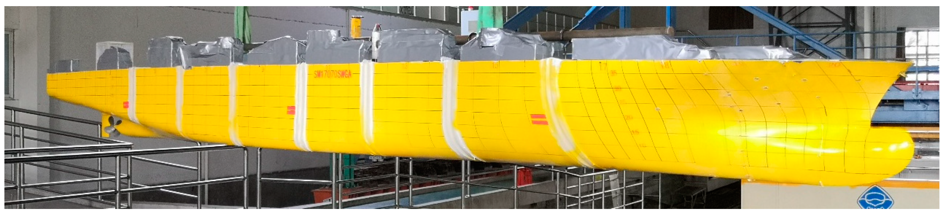
The large containership is converted into a test model according to the scale ratio λ = 1/77. The basic data are shown in

Table 1. Basic data of a large containership.

Parameter	Ship	Model (λ = 1/77)
Length between perpendiculars LBP (m)	383.0	4.974
Breadth B (m)	58.6	0.761
Depth H (m)	30.5	0.396
Aft draft Ta (m)	16.7	0.217
Fore draft Tf (m)	15.2	0.197
Displacement Δ (ton)	260,602.9	0.557
Vertical center of gravity Zg (m)	27.574	0.358
Longitudinal center of gravity Xg (m)	182.714	2.373

. The left column shows the full-scale ship data, and the right column shows the scaled model data. The test model is shown in Figure 1.

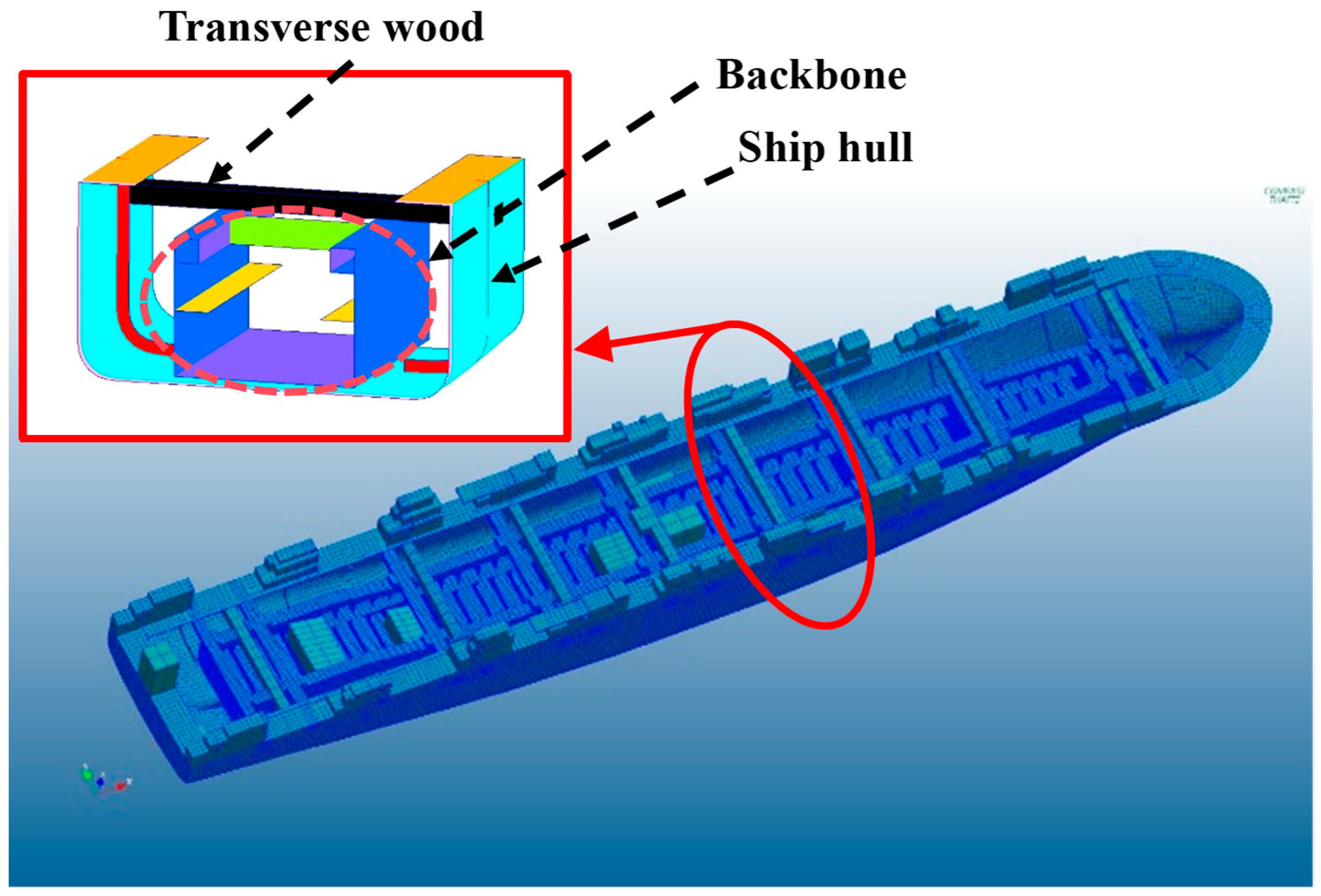
For the 1:77 scale ship model, a new type of U-shape backbone, seen in Figure 2, was designed to model the bending of the containership in waves. According to the similitude principle, a kind of ABS PC plastic plate was chosen to construct the U-shape backbone. The Young’s modulus of ABS PC is 2.4 GPa, which is about 1/85 of the steel. The Poisson ratio is 0.3897. The backbone beam in blue is connected to the ship hull through the transverse wood of a rectangular cross-section.

3.2. Numerical Setup

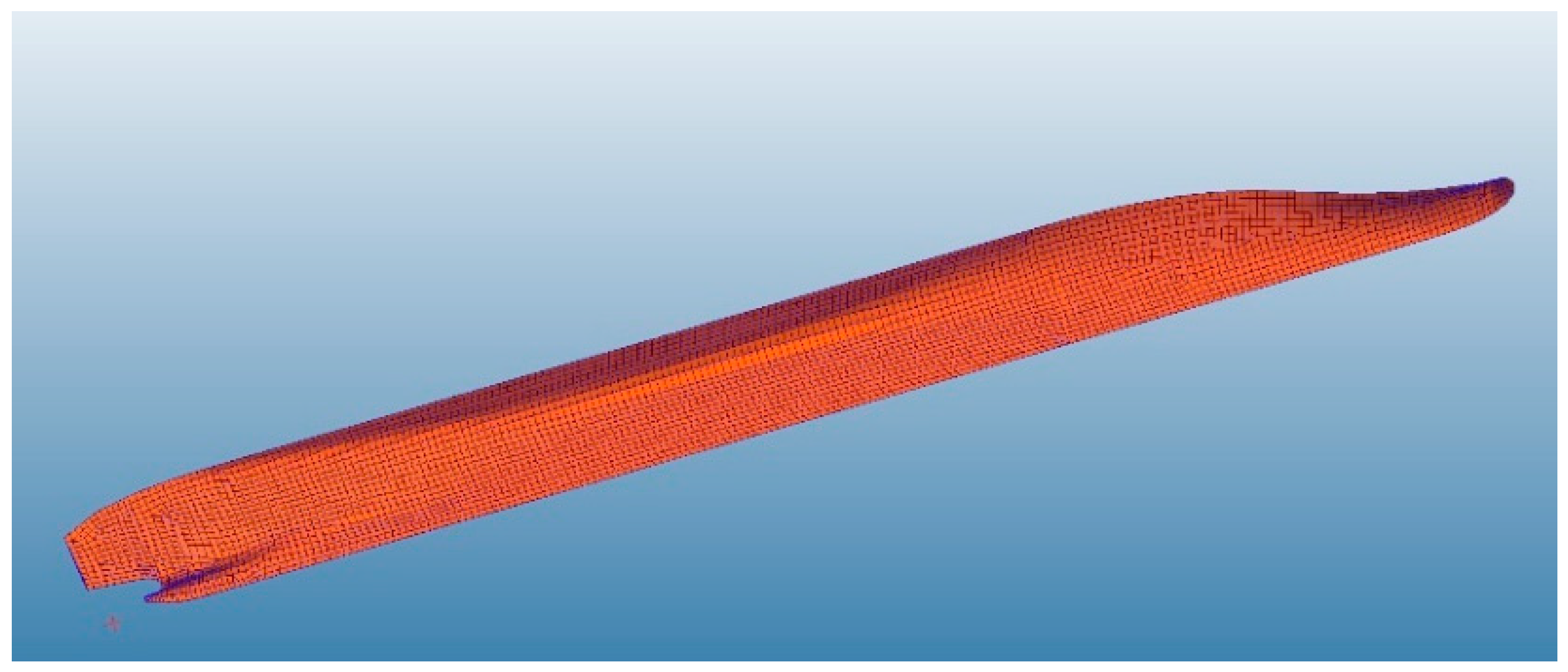
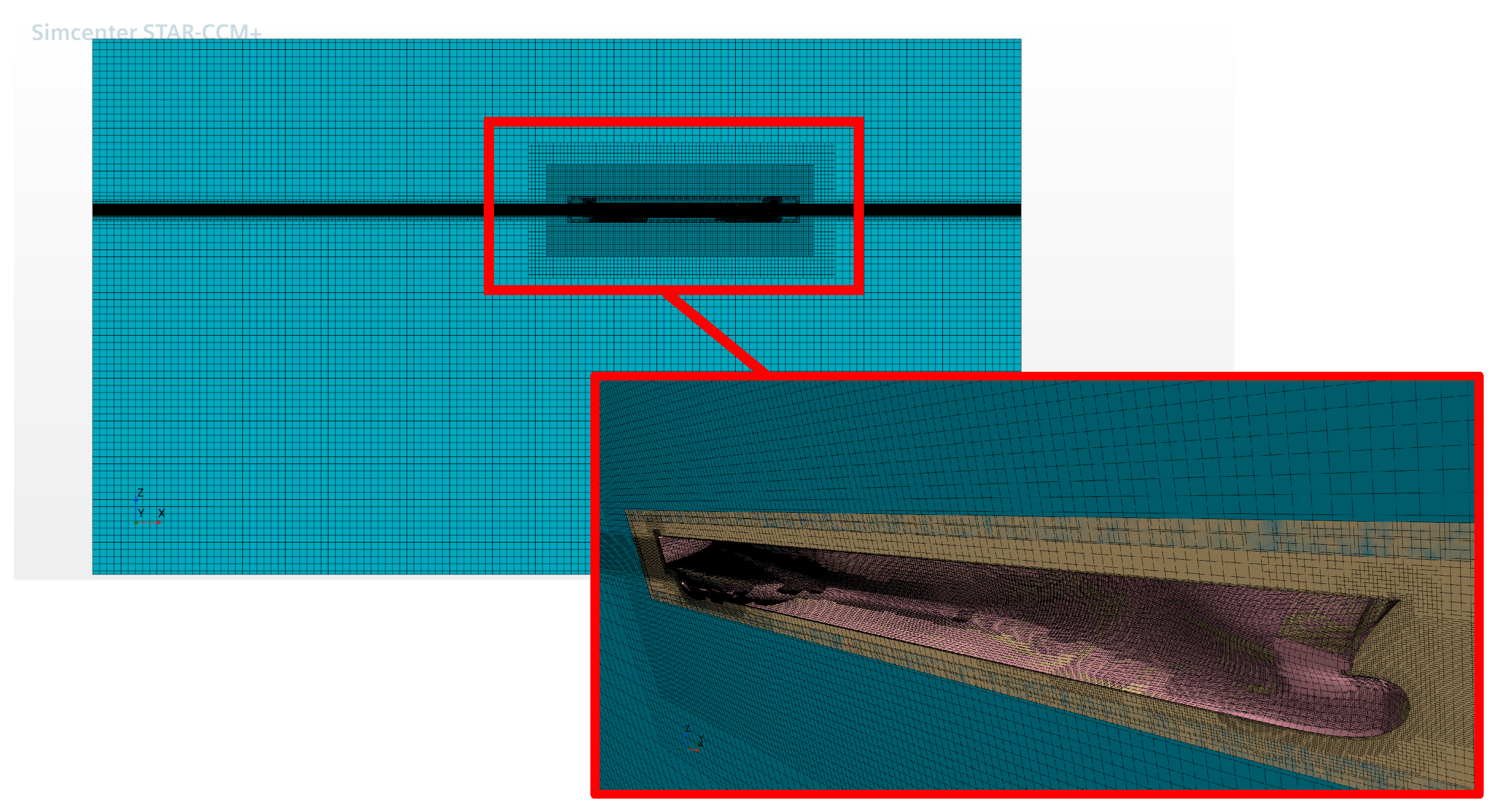
In this work, numerical simulations are conducted using the potential flow model and CFD model based on the unsteady Reynolds-averaged Navier–Stokes (RANS) equations solver. Figure 2, Figure 3 and Figure 4 illustrate the finite element structure model of the large containership, the potential flow model, and the CFD computational domain. The structure employed for the CFD-FEM coupling model satisfies the quality and stiffness distribution criteria of the hull structure, as presented in Figure 5. To accurately simulate the vibration characteristics of a hull girder, the requirements of stiffness similitude on vertical bending were met completely. In the 2D beam model, the corresponding stiffness was adjusted by changing the size of the beam cross-section.

To examine grid sensitivity, three systematically refined meshes for both the potential flow model and CFD model are employed, with a uniform refinement ratio of hi + 1/hi = 1.414, where hi and hi + 1 represent the grid spacings of two successive levels. The grid parameters for the two numerical models are summarized in

Table 2. The mesh independence study.

No.	hi/h1 (i = 1,2,3)	FD Mesh (Hull)	CFD Mesh (Hull)	CFD Mesh (Computational Domain)
1	1	2.6 × 103	1.0 × 104	2.05 × 105
2	1.414	3.7 × 103	1.4 × 104	2.9 × 106
3	2	5.3 × 103	2.0 × 104	4.1 × 106

.

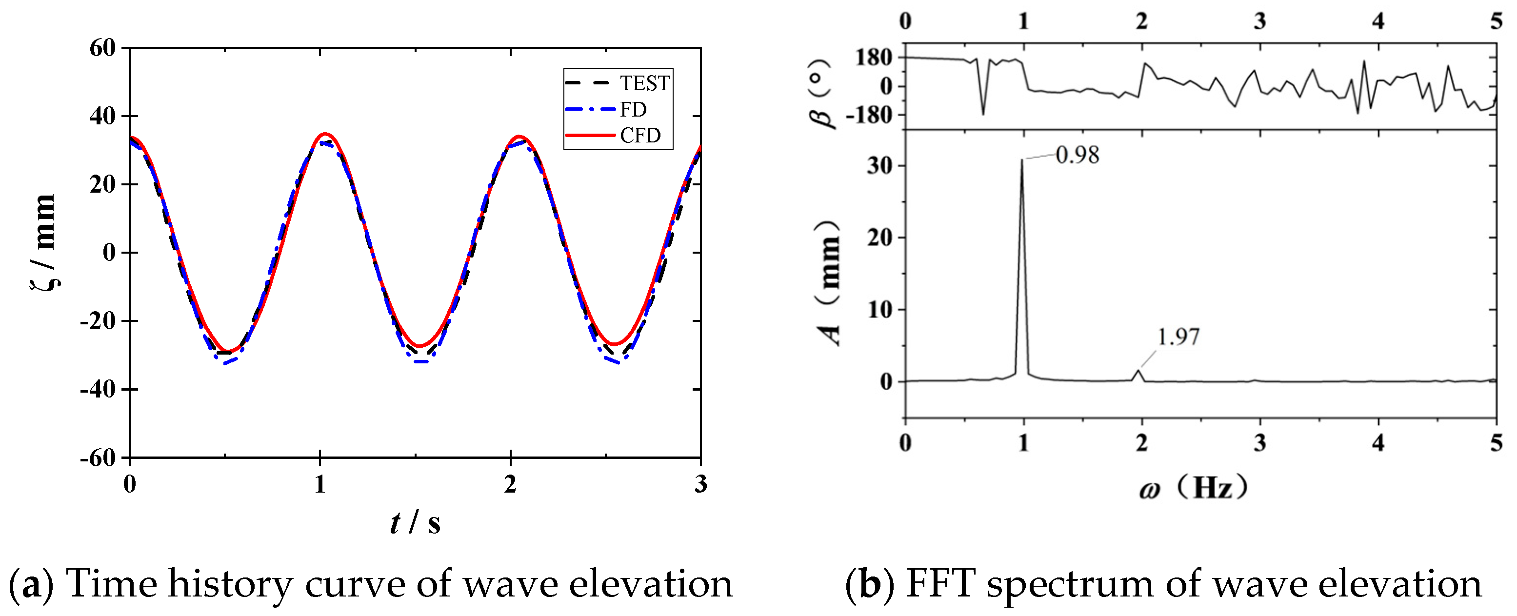
The time history curve of wave elevation with potential flow and viscous flow numerical results are depicted in Figure 6. The potential flow frequency domain calculation results in strong agreement among the three grids. In the frequency domain analysis model, the wavelength corresponding to the resonance frequency comprises a grid of at least five lengths. Grid 2 meets the calculation accuracy requirements based on the minimum number of meshes included in the minimum wavelength. As for the CFD simulation, good agreement is found among the results of Grid 2 and Grid 3, while the wave amplitude in Grid 1 is slightly reduced. The convergence ratio decreases with an increase in the mesh number, which means the numerical model is monotonically converging. According to the analysis of wave elevation, Grid 2 is selected as an appropriate resolution since the wave profiles are captured better than Grid 1, while the calculation is less demanding than Grid 3 for the CFD simulations.

3.3. Nonlinear Case

The modal shapes corresponding to this resonant frequency reveal significant vertical bending deflections at the two-node mode, indicating potential areas of concern for structural integrity. Additionally, the CFD model, as shown in Figure 4 and Figure 5, captures the complex fluid–structure interaction, enabling a more accurate prediction of the ship’s response to wave loading. This detailed modeling approach is crucial for understanding and mitigating the effects of wave-induced springing on large containerships. The resonant frequency of the vertical bending springing at two nodes of a containership model traveling in the wave basin at a speed of 23 knots (1.348 m/s at model scale) is 3.589 Hz (22.55 rad/s). The incident wave frequency that triggers this resonance is generally 9.68 rad/s, with a wavelength of 0.658 m. However, due to the constraints on maximum amplitude when generating short waves in the seakeeping tank, the incident wave frequency corresponding to half the resonant frequency of the vertical bending wave-induced vibration at two nodes, which is 6.06 rad/s (wavelength equals 1.677 m), is chosen as the wave condition for the bow wave test in the tank. For the full-speed test conditions of the containership model, refer to

Table 3. The case of ship model test for nonlinear wave-induced springing.

Case	Speed		Wave height		Wavelength		Direction (°)
	Ship (kn)	Model (m/s)	Ship (m)	Model (mm)	Ship (m)	Model (m)
No. 1	23.0	1.348	5.0	64.9	129.1	1.677	180

.

Based on linear hydroelasticity theory, and by comparing frequency domain calculations with CFD results, the table below (

Table 4. The linear springing frequency and the test condition frequency (Hz).

Item	Calculate the Frequency of Linear Springing	Wave Frequency in Test	$\mathbf{Encounters} \mathbf{Frequency} \mathbf{of} \mathbf{Model} \mathbf{Test} {\mathit{\omega }}_{\mathit{e}}$	$2 {\mathit{\omega }}_{\mathit{e}}$	Error
Values	3.589	0.98	1.80	3.60	−0.31%

) illustrates the comparison between the linear springing frequency of the containership model and the wave frequency under test conditions.

3.4. Discussion

The three-dimensional hydroelastic mechanics frequency-domain nonlinear analysis method and the CFD-FEM coupled hydroelastic method were applied to calculate the conventional vertical motion and vertical bending moment in nonlinear wave-induced vibration.

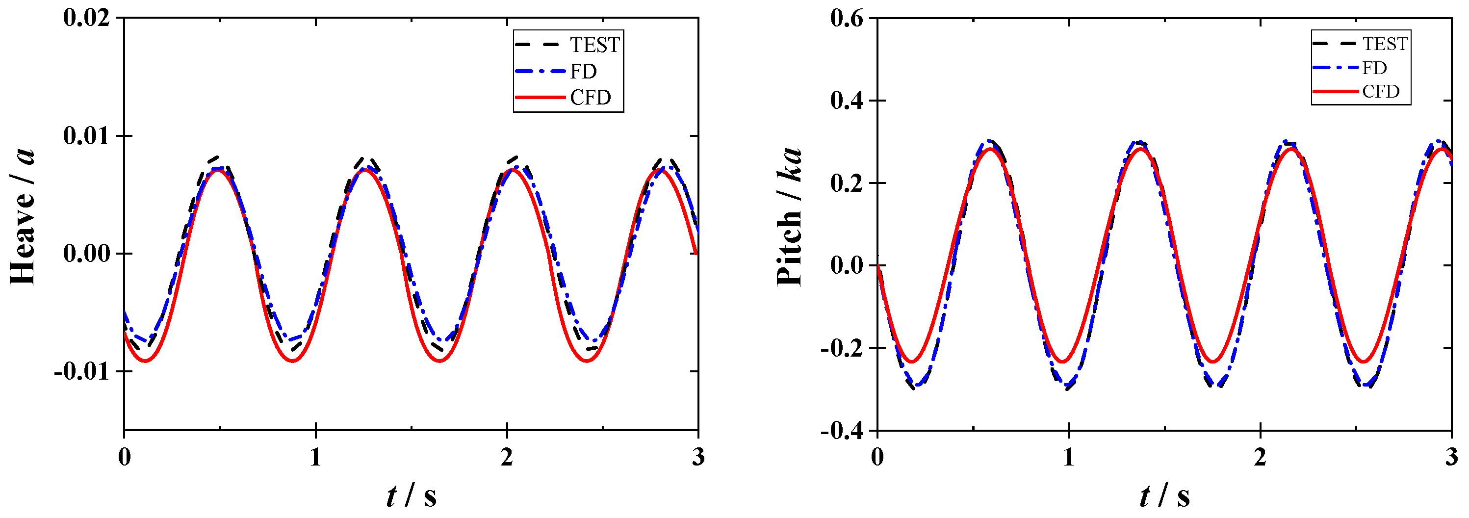
The wave height, time history of containership motion, spectrum, data analysis, and comparison with potential flow and viscous flow numerical results are depicted in Figure 7 and Figure 8. Here, “TEST” represents the test results, “FD” represents the potential flow frequency domain calculation results, and “CFD” represents the viscous flow calculation results with STARCCM+.

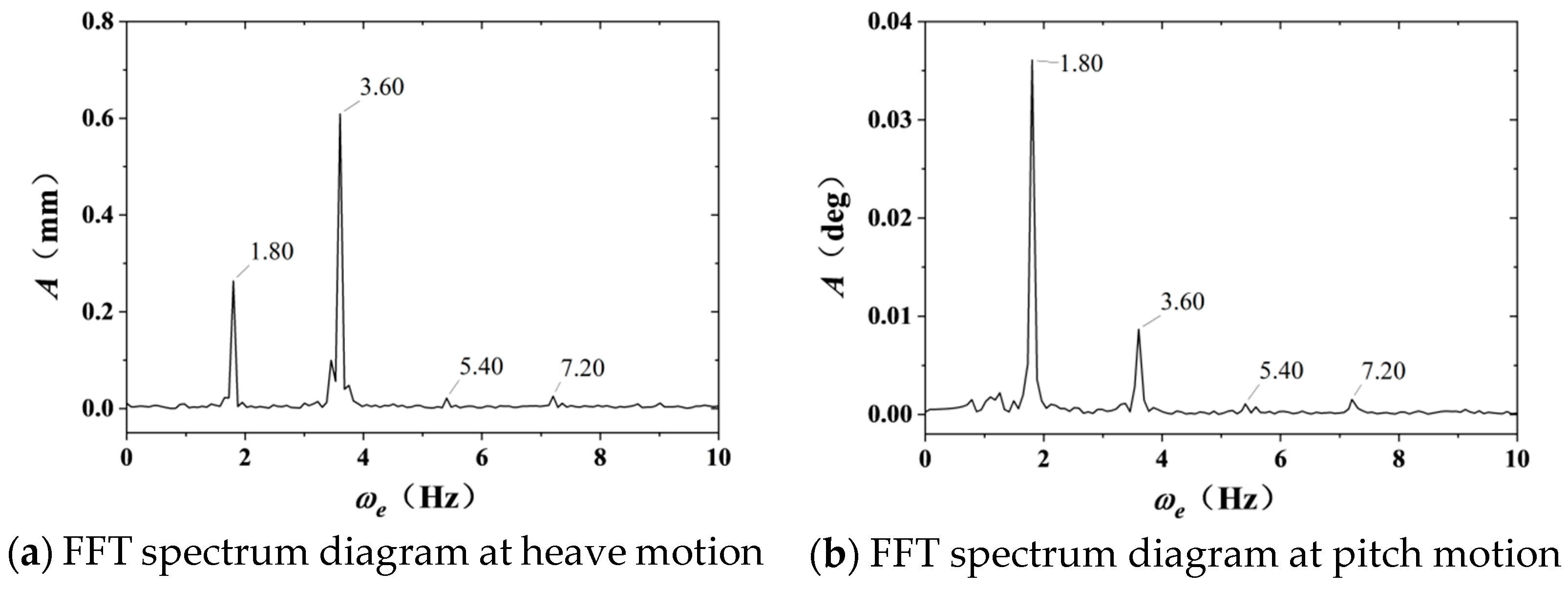
The incident wave serves as the input condition for the entire ship model measurement system, with a frequency of 0.98 Hz (wavelength 1.677 m). Nevertheless, the test wave’s high-frequency measurement information reveals a frequency of 1.97 Hz, which is twice that of the incident wave. This doubling is attributed to the unavoidable higher-order harmonic phenomenon inherent in the wave-making process within the water tank. However, these higher-order harmonics are quite minor. For wave-making, the numerical results align well with experimental outcomes, ensuring the precision of subsequent calculations. Given that nonlinear wave-induced vibrations arise from the resonant frequencies of containerships in the water, the spectrum diagram from heave and pitch measurements displays multiple vibration peaks at frequencies such as 1.80 Hz, 3.60 Hz (2×), 5.40 Hz (3×), and 7.20 Hz (4×). Among these, the encounter frequency for the containership at this speed is 1.80 Hz. Since the encounter frequency is proximate to half of the linear wave-induced vibration frequency, it is susceptible to inducing a 2× harmonic nonlinear wave-induced vibration, as per second-order nonlinear effects.

The nonlinear frequency domain hydroelastic analysis method is employed to calculate the motion and structural dynamic response of the ship model under the influence of regular waves with a frequency corresponding to the test encounter frequency within the Kelvin wave field. Additionally, the motion and section bending moment within the structure under these conditions are determined using CFD-FEM coupling calculations, as depicted in Figure 9, Figure 10 and Figure 11. Both methods demonstrated high consistency in motion and load under head wave conditions. When combined with data comparison, it is confirmed that both methods are effective for evaluating the nonlinear wave-induced vibration response of regular waves.

From the comparison of the numerical results of the large containership test model’s motions at the wave frequency shown in Figure 8 with the experimental results, it can be seen that both the frequency domain calculation method for potential flow theory and the CFD viscous flow calculation method yield numerical simulations of rigid body motion that are relatively close to the experimental results. Since the given wave incidence frequency components are fixed, the time course periods of all three methods can be effectively guaranteed. However, there are some subtle differences in amplitude, mainly due to slight variations in the damping settings of the numerical system compared to those measured in the model tests, as well as the more pronounced effect of the viscous damping term under the CFD-FEM coupling method.

Nonlinear wave-induced vibrations appear as high-frequency bending responses in the ship’s structure, resulting in higher-order harmonic components, such as those at frequencies 2× and 3×, in the motions and section vertical bending moments during operation, as shown in Figure 10 and Figure 11.

Figure 9 depicts the heave and pitch motions of the large containership over time, showcasing a comparison of results from different numerical approaches. The horizontal axis represents time t in seconds, spanning from 0 to 3 s, while the vertical axis indicates heave displacement in millimeters and pitch angle in degrees. Three distinct curves are presented as follows: -LF (red solid line) depicts low-frequency linear response, -HF (green solid line) depicts high-frequency nonlinear response, and -TF (green long-dashed line) depicts total-frequency response, respectively. This mutually validates with Figure 8, including the amplitude and frequency.

All curves exhibit periodic oscillations, which is consistent with the typical heave and pitch motion characteristics of a ship under wave excitation. However, slight differences in amplitude and phase among the curves reflect the disparities between the frequencies. Linear-based methods (e.g., Heave-LF, Pitch-LF) can only calculate and describe the responses under a single regular wave. Since the encounter frequency (1.80 Hz) under this wave is exactly half of the first-order resonant frequency (3.60 Hz) of the ship model, through the superposition of sum frequencies, the nonlinear calculated high-frequency response (e.g., Heave-HF, Pitch-HF) is exactly the response at the resonant frequency. Such comparisons are crucial for validating numerical algorithms and understanding the ship’s nonlinear springing behavior in waves, aiding in the design and optimization of containerships for better hydrodynamic performance.

As the frequency of wave encounters and its multiples coincide with the resonant frequencies of the ship’s structure after accounting for fluid-added mass, nonlinear wave-induced vibrations are triggered by waves. Considering the section vertical bending moment (VBM) as an example, as illustrated in Figure 11, the outcomes of the nonlinear frequency-domain hydroelastic analysis, which employs potential flow theory, are quite close to the experimental data. Nevertheless, due to phase differences in the low-frequency and high-frequency responses, the coupled CFD-FEM calculation method exhibits some discrepancies in the combined response.

4. Conclusions

This study systematically employs nonlinear frequency-domain hydroelastic theory and the CFD-FEM coupled hydroelastic calculation method to address the nonlinear, multi-frequency wave-induced vibration response of containerships in regular waves, with comprehensive validation against self-propelled model tests.

Specifically, the research focuses on simulating the design-speed head wave scenario in a wave basin, where motion and load response curves are acquired through experimental measurements. By implementing spectral analysis and time-history band-pass filtering, the response components are decomposed into low-frequency (wave frequency) and high-frequency (wave frequency multiples, i.e., springing resonance frequency) parts, enabling a detailed discussion of vibration mechanisms.

Based on potential flow theory, the three-dimensional frequency-domain nonlinear hydroelastic analysis method considers the second-order hydrodynamic effects induced by large-angle rigid-body rotations and instantaneous wet surface variations. In contrast, the CFD method can effectively account for the nonlinear factors of the flow field. By coupling with the FEM to solve the ship’s hydroelastic problem, not only can the effects of instantaneous wet surface and large angle rotation on the second-order wave forces in potential flow theory be captured, but also the effects of structural deformation on the flow field can be further carefully considered. Thus, the CFD-FEM coupling approach integrates the finite volume method (VOF) for free-surface capture and dynamic FEM for structural response, achieving two-way fluid–structure interaction.

Key findings reveal that both methods demonstrate high consistency in predicting vertical heave/pitch motions and vertical bending moments (VBMs) under head waves. Notably, these two numerical methods show superior accuracy in capturing nonlinear phenomena, such as high-frequency harmonic components (two times and three times of wave frequencies) in VBM responses, which arise from the resonance between encounter frequencies and structural natural frequencies (e.g., 1.80 Hz encounter frequency triggering 3.60 Hz springing resonance).

Experimental validation confirms that the frequency-domain method based on potential flow theory efficiently predicts rigid-body motions, while CFD-FEM coupling better accounts for viscous damping effects and structural-deformation-induced flow field changes. The discrepancy in combined responses (low-frequency + high-frequency) between methods is attributed to phase differences in dynamic responses, highlighting the necessity of integrating both approaches for comprehensive fatigue assessment. These results establish the effectiveness of nonlinear hydroelastic analysis and CFD-FEM coupling in evaluating wave-induced springing, providing critical technical support for hydrodynamic design optimization and fatigue strength evaluation of ultra-large containerships in severe sea conditions. Additionally, the frequency-domain nonlinear method has a fast calculation speed, making it more suitable for the preliminary design of large ships.