Spatial Sequential Matching Enhanced Underwater Single-Photon Lidar Imaging Algorithm

Abstract

Traditional LiDAR and air-medium-based single-photon LiDAR struggle to perform effectively in high-scattering environments. The laser beams are subject to severe medium absorption and multiple scattering phenomena in such conditions, greatly limiting the maximum operational range and imaging quality of the system. The high sensitivity and high temporal resolution of single-photon LiDAR enable high-resolution depth information acquisition under limited illumination power, making it highly suitable for operation in environments with extremely poor visibility. In this study, we focus on the data distribution characteristics of active single-photon LiDAR operating underwater, without relying on time-consuming deep learning frameworks. By leveraging the differences in time-domain distribution between noise and echo signals, as well as the hidden spatial information among echo signals from different pixels, we rapidly obtain imaging results across various distances and attenuation coefficients. We have experimentally verified that the proposed spatial sequential matching enhanced (SSME) algorithm can effectively enhance the reconstruction quality of reflection intensity maps and depth maps in strong scattering underwater environments. Through additional experiments, we demonstrated the algorithm’s reconstruction effect on different geometric shapes and the system’s resolution at different distances. This rapidly implementable reconstruction algorithm provides a convenient way for researchers to preview data during underwater single-photon LiDAR studies.

1. Introduction

Visible light imaging often struggles to provide reliable results in environments with extremely low visibility. Light Detection and Ranging (LiDAR) technology utilizes the time of flight of reflected light signals to determine the distance of objects [1]. Compared to Radio Detection and Ranging (RADAR) methods, LiDAR systems typically offer higher-resolution imaging of distant objects due to the use of shorter wavelengths [2]. LiDAR has unique advantages over visual imaging, but active laser imaging systems suffer from severe absorption and scattering by scattering media when operating in foggy or underwater environments with extremely low visibility [3]. The strong absorption of photon energy by scattering media can attenuate the echo signal to a weak signal at the single-photon level under extreme conditions. Single-photon avalanche diode (SPAD) detectors combined with Time-Correlated Single-Photon Counting (TCSPC) technology for imaging are a common method to address this issue [4,5,6]. Single-photon LiDAR offers photon-level detection sensitivity and picosecond temporal resolution, providing not only the intensity information but also the distance dimension information of the target [7]. Research utilizing this technology has been successfully demonstrated in various challenging scenarios, including long-range depth imaging [8,9,10], cluttered imaging [11], non-line-of-sight detection of targets hidden from view [12,13,14], and imaging of targets in highly scattering media [4,15,16]. Due to the strong scattering effect of the media, a large number of photons move backward and return directly to the system, introducing very strong backscatter noise, which makes it difficult to distinguish the echo signals of distant targets [17]. The received signal has a low signal-to-noise ratio and loss of target information [18], and these challenges severely limit the application of LiDAR in underwater environments for target detection and recognition [19].

To address the suppression of echo signals by high-intensity backscatter noise, time-gated technology has been proposed [20,21,22], which can achieve long-range imaging in scattering media. However, this method requires prior information such as known target distances and cannot effectively detect targets with unknown distances. To tackle this issue, Satat et al. proposed a probabilistic method for estimating the distribution parameters of scattering media from data [16], which is based on the differences in time-domain signal distribution to achieve photon counting imaging in scattering media and image reconstruction at the signal level. In the same year, Li et al. proposed a statistical “one-to-one” deep learning technique [23] that can capture the statistical information in the intensity pattern in a set of fixed scattering media with the same macroscopic parameters, thereby realizing imaging through scattering media. The network structure resembles U-Net [24], which has a large computational load and is designed for visible light two-dimensional imaging, not fully utilizing the information in LiDAR data. Furthermore, to address the issue of low image quality caused by scattering effects, techniques such as wavefront shaping [25], phase conjugation [26], transmission matrix [27], and speckle autocorrelation [28] have been proposed. Although these methods perform well for imaging in weakly scattering media, they exhibit poor results in strongly scattering or dynamically changing scattering media. Sun et al. proposed a class-based deep learning image reconstruction algorithm [29], which first classifies the blurred scattering images according to the scattering conditions and then reconstructs the images. This method adopts an approach from the field of computer vision for visible light images, not fully utilizing the distribution characteristics of signals and noise in the original time-domain signals, and has long training times and insufficient real-time performance of the algorithm.

In addressing these challenges, our research concentrated on the disparities in the temporal distribution of echo signals and noise. Previous research on photon counting imaging in scattering environments has established that the target reflected echo signals and the backscatter noise have distinct temporal distribution characteristics [16,30]. Building on our previous sequential two-mode fusion (STMF) imaging algorithm [31], we propose a new underwater single-photon lidar reconstruction algorithm: the SSME imaging algorithm, which can be quickly implemented without using any deep learning techniques by integrating the spatial relationship between echo signals at different pixel positions. This paper also introduces an underwater active imaging system based on the single-photon Time of Flight (ToF) method, capable of acquiring intensity and depth distribution of objects beyond the line of sight in turbid water. The system structure is coaxial transmission and reception, using a 532 nm pulsed laser light source with a maximum average optical output power of 150 mW, and the sensor is a single-pixel SPAD detector. Combined with the proposed SSME algorithm, this system can quickly achieve real-time preview of the data collected by the hardware system with a resolution of about 6 mm at a distance of 11 m in relatively turbid water. Compared with the previous research on the STMF algorithm, the lateral resolution is greatly improved, and the distance resolution is further improved. More comprehensive imaging tests are carried out on more geometric targets under more suitable experimental conditions, further improving the imaging quality.

2. Methods

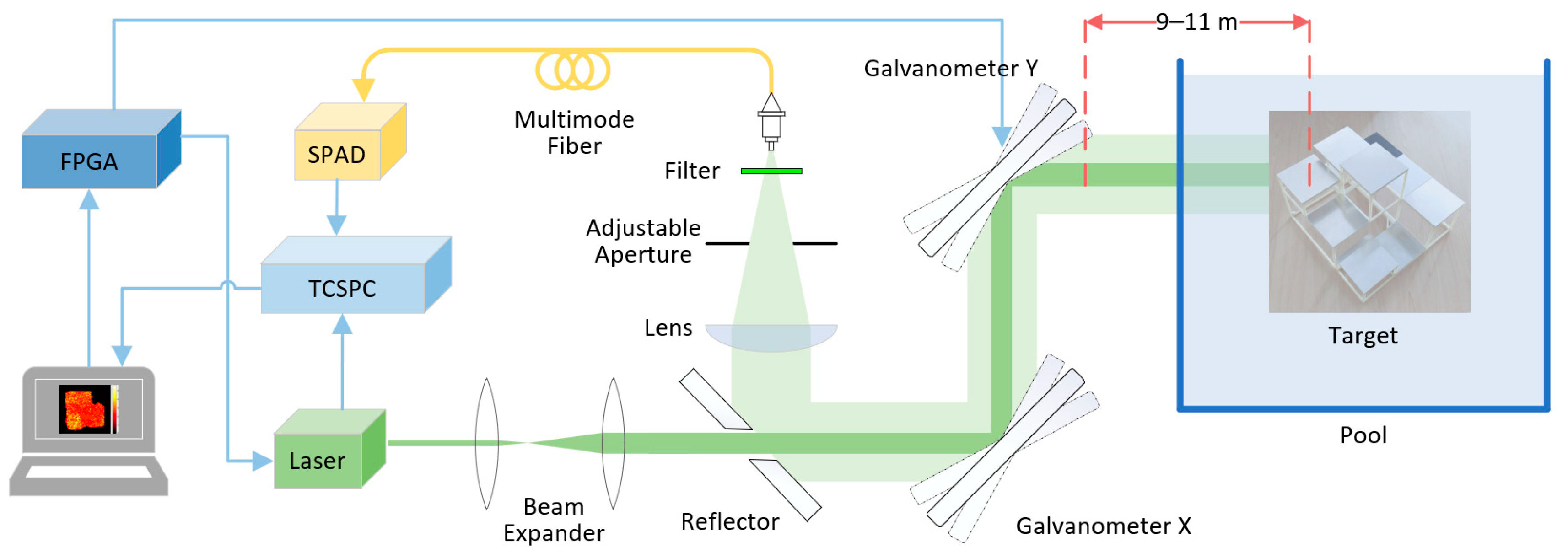
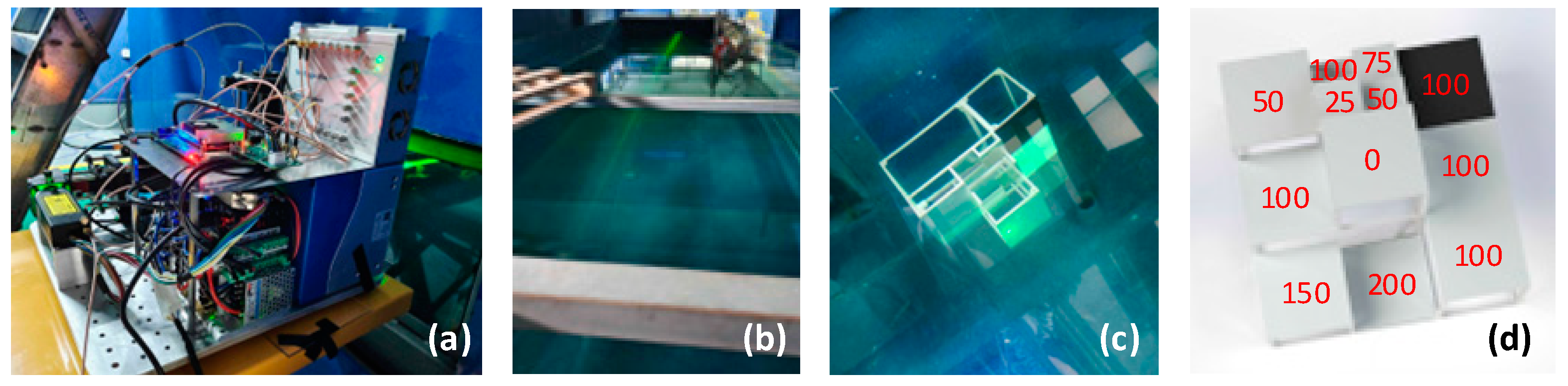
2.1. The Experiment System and Layout

The experimental system consists of an underwater single-photon LiDAR imaging system and an experimental pool. The composition of the LiDAR imaging system is shown in Figure 1. Initially, the laser is triggered by a field-programmable gate array (FPGA), and the photodiode within the laser head provides a synchronization signal to the TCSPC module for calculating the photon flight time. The laser is a sub-nanosecond passively Q-switched laser that emits a pulsed laser beam with a wavelength of 532 nm upon receiving the trigger signal. After the laser beam passes through a beam expander, the beam diameter increases and the divergence angle decreases. It then reflects off a holey mirror and a two-axis galvanometer mirror before entering the experimental pool through a glass window. The pool has a volume of 12 × 3 × 1.5 m³, and the window size is 30 × 30 cm². The test target is made using a 3D-printed frame, aluminum plates, etc., and consists of a chessboard pattern at different depths, as detailed in Section 3.1. One square is covered with a black PVC board, while other areas are covered with aluminum plates. The reflectivity of smooth aluminum plates decreases due to oxidation in air and water, reaching a stable value after a period of time. The reflectivity measured by the C84-III reflectometer is 67.2%. The target is placed approximately 9–11 m away from the glass window, with the background being the rough inner wall of the pool with extremely low reflectivity. After the echo signal reflects back from the target to the system, it passes through a bandpass filter and is then focused and coupled to a multimode fiber by a plano-convex lens. The SPAD detector uses a fiber-coupled interface and immediately generates an electrical signal upon receiving a photon. The TCSPC receives several electrical signals from the SPAD detector between two synchronization signals and calculates the time difference between each SPAD signal and the synchronization signal, ultimately generating a statistical histogram. The scanning imaging resolution is set to 64 × 64 and 128 × 128 pixels. Detailed parameters are listed in

Table 1. Summary of main parameters.

Parameter	Comment
Environment	• Unfiltered tap water • Unfiltered tap water with different concentrations of Maalox
Target stand-off distance	~9, 10, 11 m in water
Laser system	sub-nanosecond passively Q-switched laser MCC-532-5-030
Illumination wavelength	532 nm
Laser repetition rate	5 kHz
Average optical power	150 mW
Single pulse energy	~30 μJ
Laser spot diameter at target	~8 mm diameter
Optical field of view	~42 mm diameter at 9 m
Single pixel emission times used in these experiments	10 times/pixel 50 times/pixel 500 times/pixel
Histogram length	150 bins
Bin width	100 picoseconds
Detectors	Single-Photon Avalanche Diode Detector SPCM-AQRH-14-FC, 1 pixel

and more details about the hardware system are given in the “Methods” section.

To simulate water of different turbidities under natural environmental conditions, we added unfiltered tap water to the pool and then changed the turbidity of the water by adding Maalox, a commercially available antacid that strongly affects scattering without causing significant light absorption, according to [4]. Due to the large volume of the pool, to ensure as uniform a turbidity as possible throughout the water, we employed a circulating water pump to expedite the dispersion of Maalox. Before each measurement, the water pump was activated for a period to ensure proper mixing. Subsequently, the attenuation coefficient was measured multiple times at different positions along the laser beam path, and the average value was taken. The target was suspended at various positions in the pool using fine wires, approximately 9 m, 10 m, and 11 m away from the system. Experiments were conducted in water with four different attenuation coefficients: 0.42 m⁻¹, 0.56 m⁻¹, 0.67 m⁻¹, and 0.78 m⁻¹, with the overall Attenuation Length (AL) ranging from 3.8 to 8.6 AL.

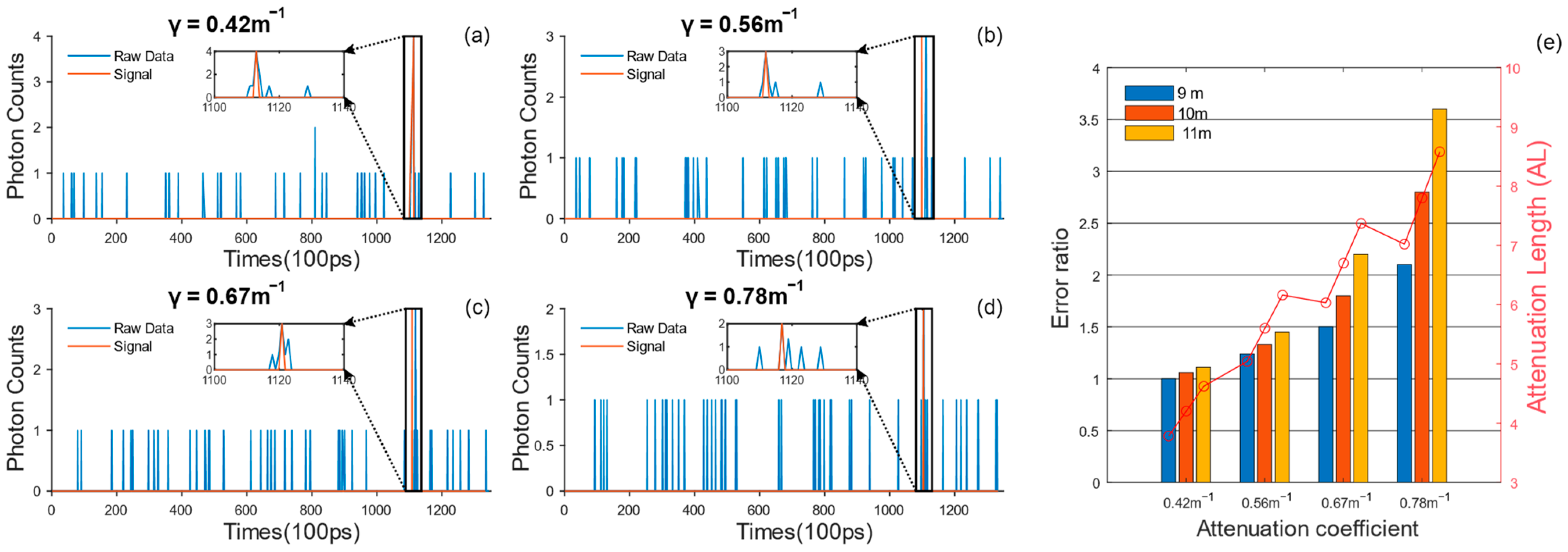
2.2. Attenuation Measurement and Evaluation Metrics

To quantitatively measure the attenuation coefficient of the water, referring to the method in [4], we used a reflector and a laser power meter to measure the optical power of a 532 nm laser at various distances, ensuring uniformity with a water pump while keeping other conditions consistent as described earlier. By taking multiple measurements, we calculated the attenuation coefficient corresponding to the current turbidity of the water. Specifically, during the transmission of the beam in water, the reflector is used to deflect the beam by 90 degrees vertically upward out of the water at different transmission distances. Then, the laser power meter is used to measure the optical power at the current position. The attenuation coefficient of the water can be calculated according to Equation (1) [32]:

$$Attenuation Coefficient\left(\gamma \right)=-{\displaystyle \frac{1}{L}}\times \mathit{ln}\left({\displaystyle \frac{E_L}{E_t}}\right)$$

(1)

where $L$ is the difference in distance between the two power measurements, $E_t$ is the initial energy of the beam, which is the power at a position closer to the system, and $E_L$ is the residual energy after the beam has propagated over a longer distance.

Additionally, to quantitatively assess the reconstruction results of the SSME algorithm, we employed the Peak Signal-to-Noise Ratio (PSNR) and the Structural Similarity Index (SSIM) to evaluate the quality of the imaging results. The mathematical expression for PSNR is given by Equation (2) [33]:

$$\mathrm{PSNR}=10\times {log}_{10}{\displaystyle \frac{MA{X}^2}{\frac{1}{N_x\times N_y}{\sum }_{i=1}^{N_x}{\sum }_{j=1}^{N_y}{\left[d\left(i,j\right)-\widehat{d}\left(i,j\right)\right]}^2}}$$

(2)

where $MAX$ represents the maximum pixel value in the image, $N_x$ and $N_y$ are the numbers of pixels in the horizontal and vertical directions of the image, respectively, $d\left(i,j\right)$ is the intensity value of the pixel at position $\left(i,j\right)$ in the reconstructed result image, and $\widehat{d}\left(i,j\right)$ is the intensity value in the ground-truth image.

SSIM, which stands for Structural Similarity Index, is a metric used to measure the similarity between two images, focusing primarily on the structural information of the images while also considering the effects of luminance and contrast. The mathematical expression for SSIM is given by Equation (3) [33]:

$$\mathrm{SSIM}\left(X,Y\right)={\displaystyle \frac{\left(2{\mu }_X{\mu }_Y+C_1\right)\left(2{\sigma }_{XY}+C_2\right)}{\left({\mu }_X^2+{\mu }_Y^2+C_1\right)\left({\sigma }_X^2+{\sigma }_Y^2+C_2\right)}}$$

(3)

where $X$ and $Y$ represent the original and reconstructed images, respectively. ${\mu }_X$ and ${\mu }_Y$ are the mean pixel values, ${\sigma }_{XY}$ is the covariance, ${\sigma }_X^2$ and ${\sigma }_Y^2$ are the variances of the original and reconstructed images, respectively. $C_1$ and $C_2$ are constants used to maintain computational stability. The value of SSIM ranges from 0 to 1, with a value closer to 1 indicating a stronger similarity between the two images and better preservation of structural information.

2.3. Noise and Echo Signal Distribution Characteristics

When LiDAR images targets within strongly scattering media, the received photon signals are primarily composed of two parts: backscattered photons and echo photons. There are also various types of noise with lower intensities, among which dark count noise is relatively more significant. The intensity of dark count noise is usually in the range of tens to thousands of Hz, determined by the parameters of the detector. However, these noises with lower intensities have a relatively minor impact on the final imaging quality and can be approximated as negligible. Due to the presence of Rayleigh scattering and Mie scattering, as the laser propagates underwater, it is continuously scattered by water molecules and other particulates in the water. The scattered photons propagate in a more comprehensive range of directions [34,35], leading to a considerable portion of the scattered photons being directly returned to the system due to water scattering. Reference [16] proposes that the transmission distance of photons between two consecutive scattering events follows an exponential distribution; hence, the time ${\tau }_i$ between two consecutive scattering events also follows an exponential distribution $({\tau }_i\sim \mathit{exp}({\mu }_s))$, where ${\mu }_s$ represents the frequency of scattering occurrences. After multiple scatterings, the system receives photons with a total flight time $T={\sum }_{i=1}^n{\tau }_i$. Each scattering is independent of the others and follows a gamma distribution $\left(T\sim Gamma\left(k,{\mu }_s\right)\right)$, where $k$ and ${\mu }_s$ represent the shape parameter and the rate parameter, respectively. The probability of detecting a scattered photon at time $t$ is defined as $f_T\left(t|B\right)$, as shown in Equation (4) [16]:

$$f_T\left(t|B\right)={\displaystyle \frac{{\mu }_s^k}{\Gamma \left(k\right)}}{t}^{\left(k-1\right)}\mathit{exp}(-{\mu }_{s}t)$$

(4)

where $k$ and ${\mu }_s$ are related to the physical properties of the highly scattering medium, and $\Gamma \left(k\right)$ is the gamma function.

The echo photons reflected back from the target are mostly ballistic photons; hence, the echo signal photons follow a distribution that is similar to a Gaussian distribution [17]. The probability of detecting a signal photon at time $t$ is given by $f_T\left(t|S\right)$[16]:

$$f_T\left(t|S\right)={\displaystyle \frac{1}{\sqrt{2\pi {\sigma }^2}}}\mathit{exp}\left[-{\left({\displaystyle \frac{t-\mu }{\sigma }}\right)}^2\right]$$

(5)

where the mean $\mu$ is related to the distance of the object, and the variance ${\sigma }^2$ is associated with the pulse broadening effect when photons undergo multiple scatterings before returning to the system.

Due to the significant differences in the probability distributions of backscattered photons and echo signal photons in the time domain, it is possible to distinguish between the two in the time domain, thereby enabling the extraction of the echo signal. However, when the object is at a considerable distance, the intensity of the echo signal is extremely low, the number of echo photons is minimal, and the signal-to-noise ratio is very low. How to rapidly reconstruct images in such extreme environments is a challenge.

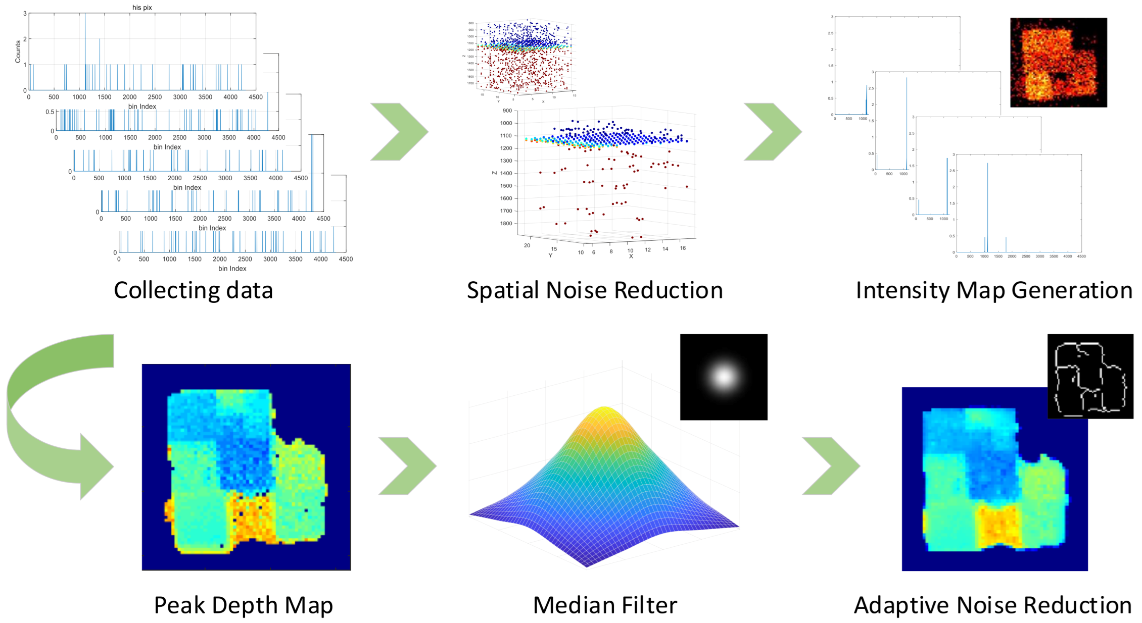
2.4. Reconstruction Algorithm

The schematic diagram of the SSME algorithm proposed in this paper is shown in Figure 2. Initially, data are collected from a preset area, and the original two-dimensional list data collected serially from all pixels are transformed into three-dimensional voxel format data. The nearest neighbor search is performed on non-zero voxels to filter out isolated voxels, completing preliminary noise reduction. Subsequently, as needed, the histograms of all pixels are accumulated, and based on statistical characteristics, the depth range where the target object is located is adaptively selected, filtering out noise data outside the depth range. Since the number of echo photons from a single pixel is small, and intensity-similar noise is introduced near the object edge due to water scattering, which severely affects the imaging quality, the matched filtering algorithm is used to generate an intensity map mask to screen and filter out other scattered noise pixels. Depth information is extracted using the peak value method, and abnormal pixels are repaired. Finally, an adaptive Total Variation (TV) smoothing constraint algorithm is used to perform smoothing denoising with different intensities for different regions of the image to preserve sufficient high-frequency details and enhance the overall imaging quality. The SSME algorithm interpretation is shown in Algorithm 1.

Algorithm 1 SSME algorithm interpretation

Input: scan_resolution, bins, bin_width, data_histogram

Output: Intensity_map, Depth_map

//Data preprocessing and filtering

$\hspace{1em}{N}_{x,y,z}\leftarrow N_i,T_i$

for all $voxel$ in $N_{x,y,z}$ do

$\begin{array}{c}voxel=0 if \left[\left({\displaystyle \sum _{i=x-1}^{x+1}} {\displaystyle \sum _{j=y-1}^{j+1}} {\displaystyle \sum _{k=z-1}^{z+1}} voxe{l}_{i,j,k}\right)-voxel=0 \& voxel !=0\right]\end{array}$

end for

//Matched filtering and mask generation

for all $n_{x,y,\tau }$ in $N_{x,y,z}$ do

${ I}_{x,y}=max\left[{\int }_{ 1}^{bins} n_{x,y,\tau }h\right(z-\tau \left)d\tau \right]$

end for

//Depth value extraction and masking

for all $N_{x,y}$ in $N_{x,y,z}$ do

$dept{h}_{x,y}\leftarrow indices\left[\mathrm{a}\mathrm{r}\mathrm{g}\mathrm{m}\mathrm{a}\mathrm{x}\right(N_{x,y}\left)\right],{ I}_{x,y}$

end for

//Denoising and adaptive TV smoothing

for all ${depth}_{x,y}$ do

$dept{h}_{x,y}^{new}\leftarrow dept{h}_{x,y}, I_{x,y}$

end for

2.4.1. Data Preprocessing

The system utilizes a serial scanning approach to sequentially scan all pixels. The raw data collected are a histogram for each pixel, with all pixel histograms collectively constituting a list. Equation (6) denotes the actual time associated with each bin, and the number of photons arriving at the corresponding time is specified by Equation (7), with $\chi$ representing the bin’s ordinal number.

$$T_i=\left\{t_i^1,t_i^2,t_i^3,\dots \dots ,t_i^{\chi }\right\}$$

(6)

$$N_i=\left\{n_i^1,n_i^2,n_i^3,\dots \dots ,n_i^{\chi }\right\}$$

(7)

After the data collection from all pixels is completed, the obtained raw data are a two-dimensional matrix with (H × W) rows and T columns, where H and W are the total number of vertical and horizontal pixels in the collection area, respectively, and T is the total number of bins in the histogram. T is also related to the duration of data collection. To facilitate subsequent data processing and readability, the two-dimensional matrix is converted into a three-dimensional voxel format. First, according to the scanning order and spatial position, each row of the list is re-sorted according to the position of the corresponding pixel. Then, based on the speed of light underwater, the third dimension is mapped to the distance dimension in real physical space. Equation (7) is transformed into the following form:

$$N_{x,y,z}=\left\{n_{x,y,1},n_{x,y,2},n_{x,y,3},\dots \dots ,n_{x,y,\chi }\right\}$$

(8)

Following the transformation of the raw data into voxel format, initial noise filtering is conducted by mapping the spatial relationships among points in the real space. Given the random characteristics of noise and the clustered distribution of echo signals from the surfaces of actual objects, there is a distinct difference in their spatial distribution, which enables the effective removal of most random noise and dark count noise. A convolution kernel is applied to perform a convolution operation on the 3D matrix $N_{x,y,z}$, with dimensions of 3 × 3 × 3, where the central element is set to 0 and all other elements are 1.

2.4.2. Peak Depth Based on Matched Filtering

The dimensions of the observed object in the range direction are usually much smaller than the measurement depth range; therefore, the data points typically exhibit characteristics of being clustered within a smaller range in the third dimension. Summing up all the $N_i$ yields Equation (9).

$$N_{sum}={\displaystyle \sum _{i=1}^{H\times W}}\left\{n_i^1,n_i^2,n_i^3,\dots \dots ,n_i^{\chi }\right\}=\left\{n_1,n_2,n_3,\dots \dots ,n_{\chi }\right\}$$

(9)

By extracting the wave packet in $N_{sum}$, the time range where the echo photons are clustered can be determined. Filtering out the noise data outside this range in the third dimension achieves dynamic range gating, which effectively enhances the signal-to-noise ratio of the echo signal from the observed object. Moreover, for objects at different depths in the foreground and background, extracting multiple depth ranges can implement multi-range gating filtering. However, while this processing can significantly improve the imaging quality, it may also overlook small-volume objects outside the selected time range. Thus, there is a trade-off here that needs to be judged based on the specific underwater environment to decide whether to enable this processing.

The matched filter is a special type of filter that maximizes the ratio of the signal’s instantaneous power to the noise’s average power at the output end by matching with an expected template signal. This allows it to be optimized for specific signals. For the echo signals returned from the object’s surface, they have a relatively stable probability distribution characteristic, which can be quickly determined through simulation and experiments. When using LiDAR hardware systems with different model components, the best ideal template signal can be quickly obtained through experiments, thereby enhancing the effect of the matched filter in the data processing process and optimizing the overall imaging quality of the system. In addition, due to the certain degree of spatial broadening effect when the laser propagates underwater, this distribution has subtle differences for the echo signals of objects at different distances. Based on the differences between the echo signals at different distances, different template signals can be adaptively used for matched filtering, thereby achieving more accurate signal extraction. According to the principle of the convolution operator, the input signal is convolved with the template signal, and the output signal is as shown in Equation (10) [36], where $n_{x,y,\tau }$ is the value of the $\tau$-th bin of a certain pixel, and $h\left(t-\tau \right)$ is the reversed sequence template signal.

$$y_{x,y}\left(t\right)={\int }_1^{\chi }{n}_{x,y,\tau }h\left(t-\tau \right)d\tau$$

(10)

Due to the significant differences between the scattering noise and background noise signals generated at the edges of objects and the template echo signal, it is easy to distinguish noise from the actual echo signal by the amplitude output from the matched filter. This allows for better extraction of the pixel area where the object is located. Conventional methods directly generate a reflection intensity map by accumulating the count values of all pixels, and the former has a significant advantage compared to the latter. After filtering out the noise pixels corresponding to non-target areas, a mask of the actual pixel area corresponding to the target is obtained. Here, we use the peak index to directly extract the depth value, rather than the peak time output by the matched filter. The reason is that in experiments, we found that when the number of echo photons is small, the peak time of the latter has a larger error compared to the true depth value. Therefore, we directly use the peak time of the data, as shown in Equation (11) [31].

$$\underset{indices}{T_{x,y}}=\mathrm{indices}[\underset{n}{\max }\left(\left\{n_{x,y,1},n_{x,y,2},n_{x,y,3},\dots \dots ,n_{x,y,\chi }\right\}\right)]$$

(11)

2.4.3. Optimizing Reconstruction Results

Due to the complex and variable nature of underwater environments, some pixels may be corrupted or missing during data collection. To further enhance the imaging quality and reduce the impact of noise, a two-step process is applied to repair these anomalies. First, isolated points are replaced with median values; isolated zero points within the target area mask are filled with the median of their neighborhood, and this process is iterated until there are no isolated zero points in the mask. Additionally, due to differences in object surface reflectivity or geometric shapes, some areas have lower echo intensities, resulting in local anomalies. These are addressed by identifying simply connected regions and filling these smaller abnormal areas with median values.

After initial denoising of the voxel data, they are filtered with the mask and the distance values are calculated using the peak value method. However, due to variations in reflectivity at different locations of the target, the presence of trace amounts of large particulate impurities in water, and measurement errors in the system, there may be significant errors in the distance values of some pixels, necessitating further correction. Additionally, to protect high-frequency information as much as possible, when using the median method, only the first-order neighborhood of the anomaly points is statistically considered, and a threshold control is added to prevent excessive smoothing. Assuming the root mean square width of the system response function is $\eta$, the spatial correlation of pixels is utilized to compare the current pixel time $T_{x,y}$ with the average $T_{x,y}^{average}$ of the 3 × 3 neighborhood. Whether to correct the depth value of the current pixel is determined by Equation (12) [31].

$$T_{x,y}^{new}=\left\{\begin{array}{cc}\underset{indices}{T_{x,y}}& , \left|\underset{indices}{T_{x,y}}-T_{x,y}^{average}\right|\le 2\cdot \eta \\ T_{x,y}^{average}& , \left|\underset{indices}{T_{x,y}}-T_{x,y}^{average}\right|>2\cdot \eta \end{array}\right.$$

(12)

The TV smoothing denoising algorithm achieves the purpose of denoising by minimizing the total variation of the image. The optimization problem can be represented by Equation (13), where $T_{x,y}^{new}$ is the input depth map for the TV algorithm, and $\widetilde{T_{x,y}^{new}}$ is the depth map after smoothing by the TV algorithm. Among them, $f\left(·\right)$is defined by Equation (14) as the magnitude of the difference between the current pixel and neighboring pixels, and $\lambda$ is used to adjust the filtering strength [31].

$$\widetilde{T_{x,y}^{new}}=\underset{\widetilde{T_{x,y}^{new}}}{\mathrm{m}\mathrm{i}\mathrm{n}}\left[\left(\widetilde{T_{x,y}^{new}}-T_{x,y}^{new}\right)+\lambda \cdot f\left(\widetilde{T_{x,y}^{new}}\right)\right], 0\le \widetilde{T_{x,y}^{new}}\le T_{x,y}^{new}$$

(13)

$$\begin{array}{c}f\left(\widetilde{T_{x,y}^{new}}\right)={\displaystyle \sum _{x=1}^{X-1}}{\displaystyle \sum _{y=1}^{Y-1}}\sqrt{{\left(\widetilde{T_{x,y}^{new}}-\widetilde{T_{x+1,y}^{new}}\right)}^2+{\left(\widetilde{T_{x,y}^{new}}-\widetilde{T_{x,y+1}^{new}}\right)}^2}\\ \hspace{1em}\hspace{1em}\hspace{1em}+{\sum }_{x=1}^{X-1}\left|\widetilde{T_{x,Y}^{new}}-\widetilde{T_{x+1,Y}^{new}}\right|+{\sum }_{y=1}^{Y-1}\left|\widetilde{T_{X,y}^{new}}-\widetilde{T_{X,y+1}^{new}}\right|\end{array}$$

(14)

Since the size of the observed object compared to the pixel size of the final imaging result and the size of the laser spot is relatively large, it can be simplified to a simple geometric shape. Compared with high-resolution visible light images, the imaging resolution of single-photon LiDAR is lower, but the amount of information per pixel is greater, representing the true distance information of that pixel. The TV smoothing algorithm is designed for visible light images. Therefore, if a single parameter $\lambda$ value is directly used to filter the depth map, two results will occur. First, when the denoising intensity is high, the shape edge area will be too blurred and too many high-frequency details will be lost, seriously affecting the accuracy of the depth value in some areas; second, when the denoising intensity is weak, it cannot significantly improve the inter-pixel ranging error caused by a very small number of echo photons, and cannot effectively improve the imaging quality.

To more effectively extract the edge information of the object, we used an improved operator based on the Sobel operator, optimized the value of the operator for underwater single-photon LiDAR data, and detected the edge areas by looking for the maximum values of the gradient in the depth image. The magnitude of the gradient indicates the strength of the edge at that point, and the direction of the gradient indicates the direction of the edge. This method has a certain robustness to noise and can detect edges in the image well. In specific implementation, two 3 × 3 matrices and two 5 × 5 matrices are used to perform convolution operations with the original image to obtain gradient images in different directions, and then the root mean square value of all gradient images is calculated as the final edge strength mask. Based on the depth information, according to the edge mask, the parameter $\lambda$ of the TV smoothing algorithm is automatically adjusted. In areas where the gradient changes gently, that is, approximate plane areas, stronger smoothing is used to reduce ranging noise. In areas where the gradient changes dramatically, that is, edge areas, weaker smoothing processing is used to enhance high-frequency components and improve the overall reconstruction quality.

3. Results

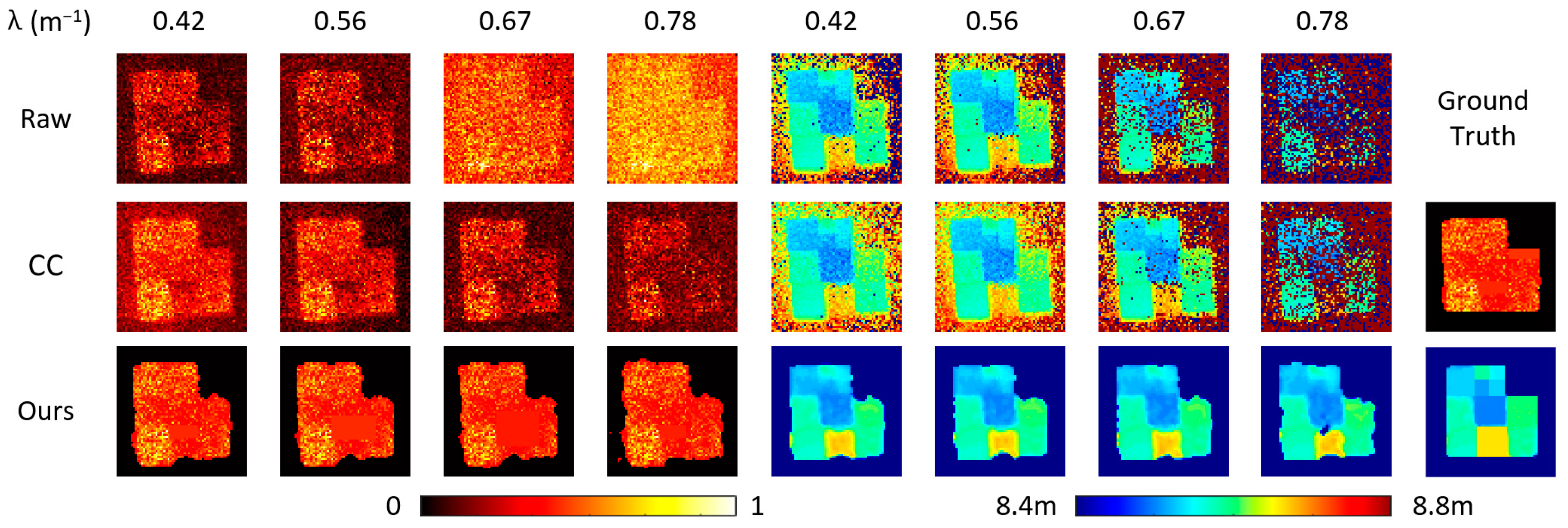
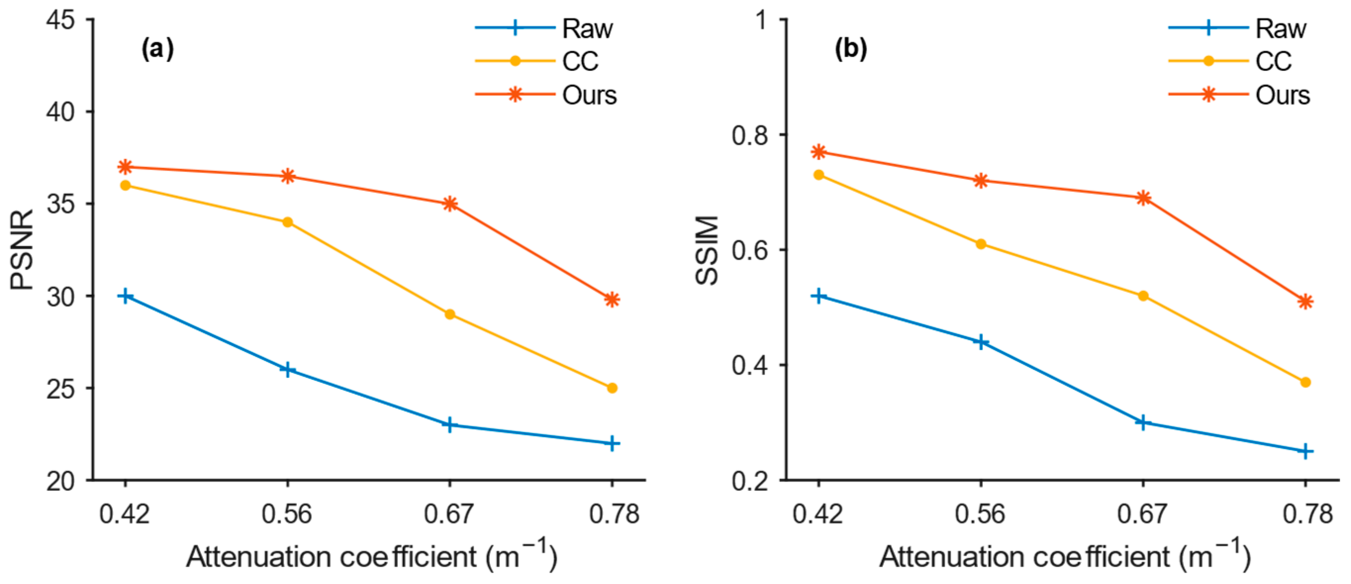
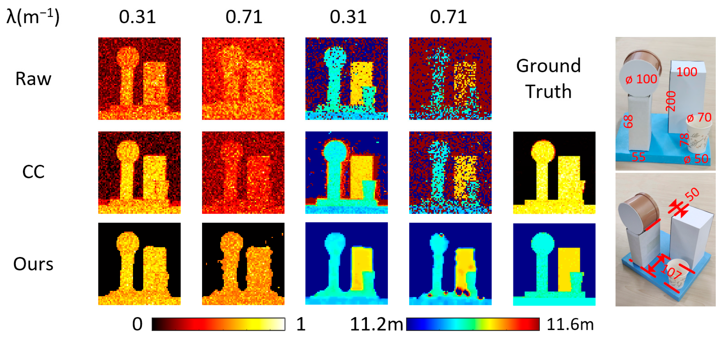
3.1. Depth Error and Reconstruction Results Under Different Turbidity

We conducted experiments in the pool to collect echo signals under varying conditions, thereby assessing our algorithm’s capability to accurately extract depth information. Echo data were collected at distances of 9 m, 10 m, and 11 m from the system, and in water with attenuation coefficients of 0.42 m⁻¹, 0.56 m⁻¹, 0.67 m⁻¹, and 0.78 m⁻¹. As shown in Figure 3a–d, as the attenuation coefficient of the water increases, scattering noise gradually intensifies, and the strength of the echo signal decreases. At an attenuation coefficient of 0.78 m⁻¹, the ranging accuracy noticeably degrades. The relative ranging errors under different distances and attenuation coefficients are shown in Figure 3e. The RMS value of the distance error at 9 m and an attenuation coefficient of 0.42 m⁻¹ is set as the reference value. It can be observed that within the tested attenuation coefficient range, the increase in distance has a smaller impact on the ranging error, while the attenuation coefficient has a greater impact. Further combined with the attenuation length of the secondary coordinate axis, it can be seen that the ranging error is closely related to the total attenuation distance.

The system is equipped with a 1 nm bandwidth pass filter and a laser with a low repetition rate of 5 kHz and high single-pulse energy. In an extreme scenario, even if only one photon signal is detected per laser pulse emission, whether it is backscattered noise or echo signal, the photon event rate remains at 5000 per second. Meanwhile, the dark count rate of the SPAD detector does not exceed 100 Hz, meaning it can produce a maximum of 100 false photon events per second, which is significantly different from the former. Under normal circumstances, the data volume of the former ranges from tens of thousands to millions per second; hence, the majority of noise in the raw data collected by the TCSPC system originates from the external environment.

Based on the depth information of individual pixels, we conducted image reconstruction experiments on targets in water with different attenuation coefficients. In a complete scan, the raw data collected by TCSPC are a two-dimensional matrix with (H*W) rows and T columns, where H and W are the pixel sizes in the horizontal and vertical directions of the image, and T is the total number of bins corresponding to each pixel. The order of the rows in this two-dimensional matrix corresponds to the order of the scanned pixels. The experimental setup and scene are shown in Figure 4, where Figure 4d shows the test target and the values of different areas represent the relative distance from the central area in millimeters. For comparison purposes, the Cross-Correlation algorithm and the proposed SSME algorithm were used for processing. The comparison of reconstruction results is shown in Figure 5.

As shown in Figure 5, in water with attenuation coefficients of 0.42 m⁻¹ and 0.56 m⁻¹, the original reflection intensity maps are relatively clear, and the pixel areas corresponding to the target can be distinctly differentiated. However, the black area in the upper right corner of the target, due to its low reflectivity, has too few effective echo photons, missing in the result. In water with attenuation coefficients over 0.56 m⁻¹, the reflection intensity maps deteriorate further, with reduced contrast and increasing blurriness. In water with attenuation coefficients over 0.78 m⁻¹, some pixels completely disappear in the depth map, making it impossible to obtain the true depth values. Moreover, as the attenuation coefficient increases, the effects of both reconstruction methods decline, with the reconstruction results exhibiting varying degrees of blurriness and missing information, but the method proposed in this paper is still better. When the attenuation coefficient is greater than 0.67 m⁻¹, the noise in the images reconstructed by the Cross-Correlation algorithm increases significantly, while our proposed SSME algorithm still maintains clear contours and better distance values.

It is worth noting that during the experimental process, we found that regardless of whether the target exists in the field of view corresponding to the pixel, the peak value algorithm can output a time. Since it is difficult to distinguish between scattering noise and echo signals in the edge areas of the target, we combined the reflection intensity map obtained by matched filtering with the depth map. By leveraging the characteristic that scattering noise pixels have low intensity in the reflection intensity map, we filtered out the corresponding pixels in the depth map. To quantitatively evaluate the reconstruction results of the target, we calculated the PSNR and SSIM of all reconstructed images, as shown in Figure 6.

From Figure 6, it is evident that the images obtained using the SSME algorithm have higher PSNR and SSIM under all attenuation coefficients and distances. The overall image quality is superior to that of the Cross-Correlation algorithm. Specifically, it was observed that the proposed method yields better results when the attenuation coefficients are 0.42 m⁻¹ and 0.56 m⁻¹. When the attenuation coefficient is 0.67 m⁻¹, the SSIM of the results obtained by the proposed method is 0.17 higher than that of the Cross-Correlation algorithm, and the PSNR is 6.21 dB higher. When imaging in water with a higher attenuation coefficient, it was found that both algorithms deviate significantly in the extracted depth values due to the weaker echo signal. The images reconstructed by our algorithm exhibit higher recognizability and better imaging quality. However, when the attenuation coefficient is too large and the water is too turbid, the number of effective echo photons per pulse is less than 1. Although accurate ranging can be achieved by increasing the number of emissions per pixel, it will significantly increase the sampling time.

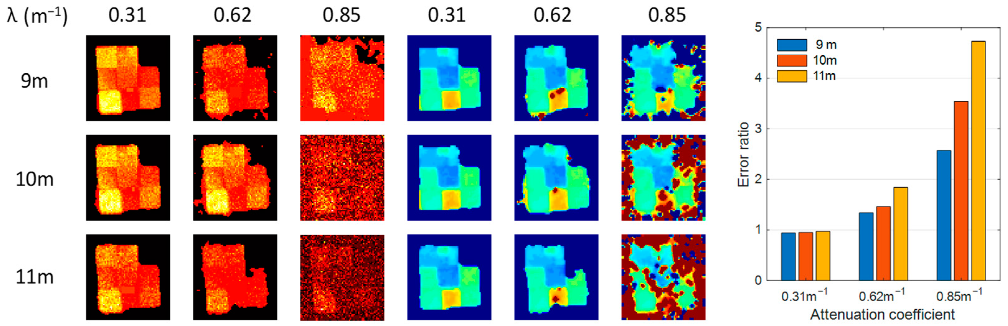
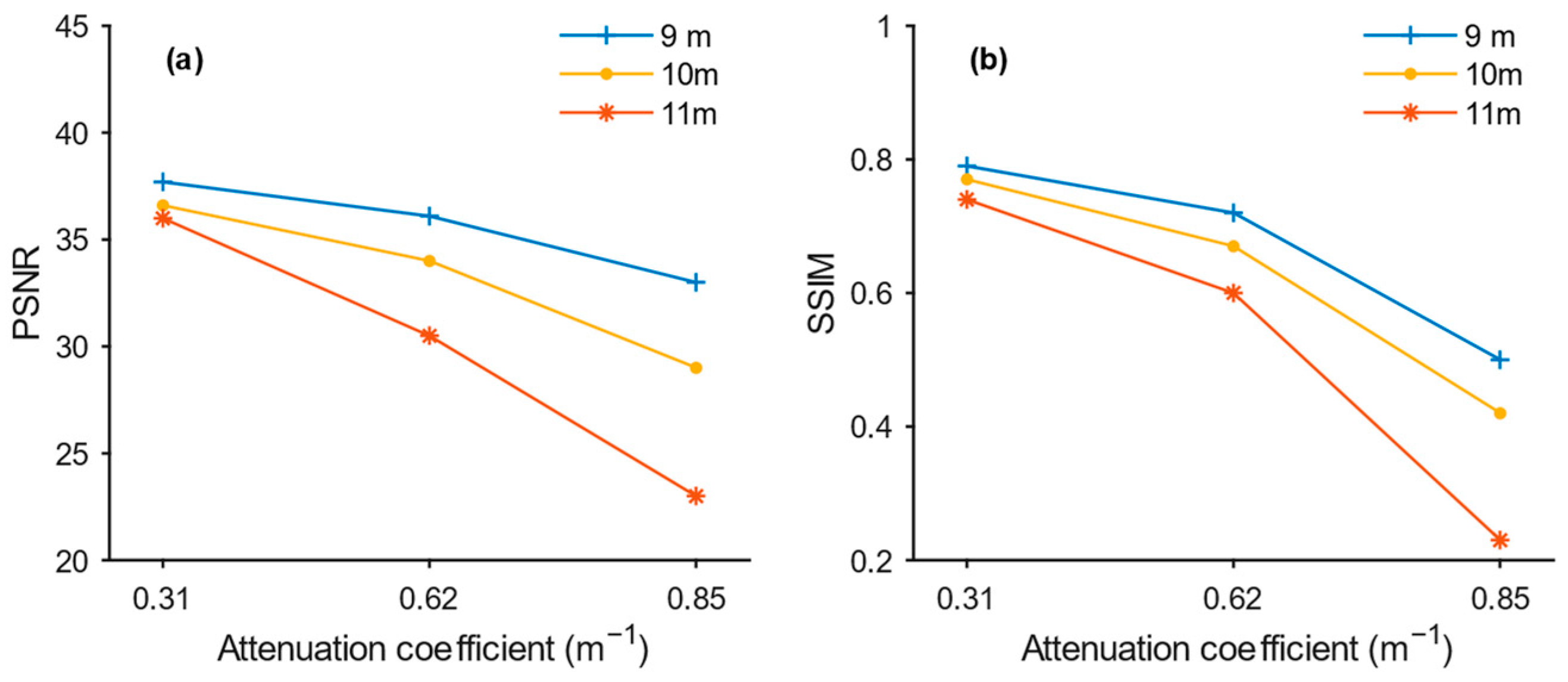
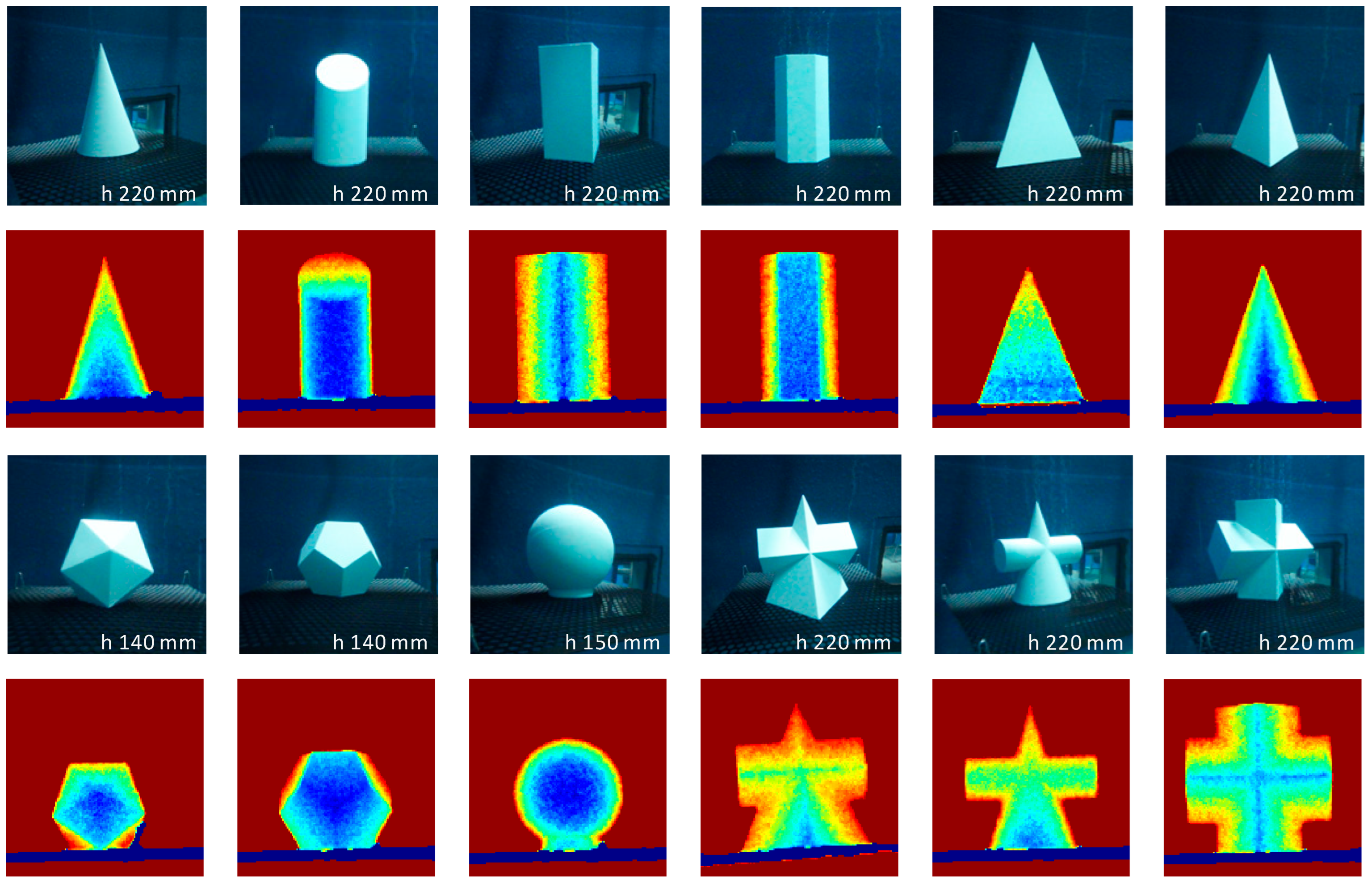
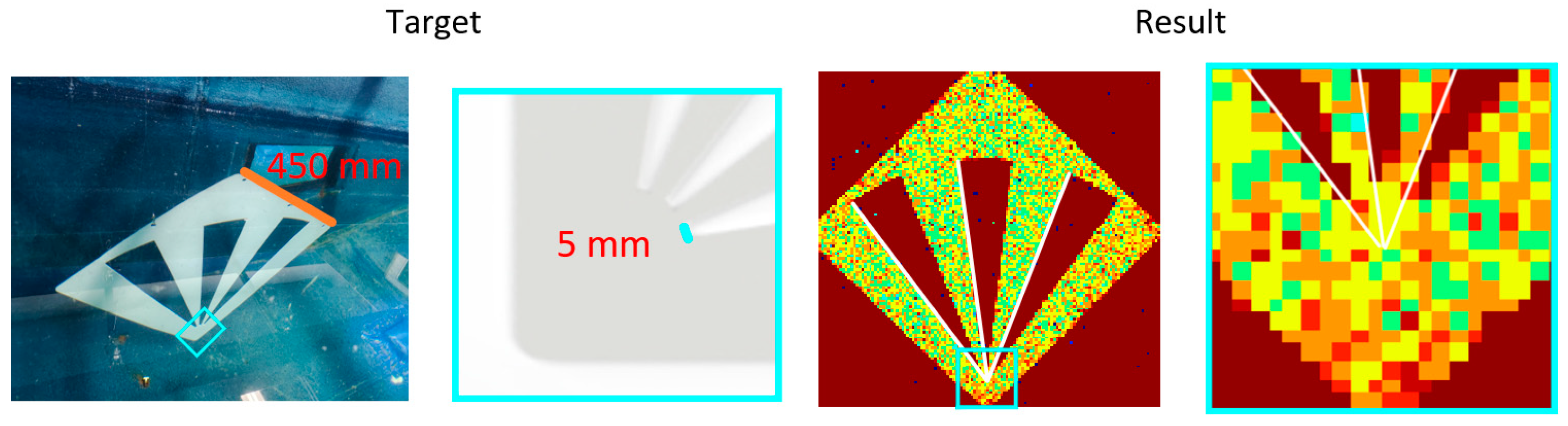
3.2. Image Reconstruction Performance Outside the Test Target

In previous studies, we designed the algorithm and carried out imaging experiments for a distance of 9 m and water with attenuation coefficients of 0.42 m⁻¹, 0.56 m⁻¹, 0.67 m⁻¹, and 0.78 m⁻¹. To test the universality of the proposed algorithm, we conducted further image reconstruction tests. These tests were beyond the scope of the targets and experimental parameters in the previous tests. Specifically, employing the SSME algorithm and parameters detailed earlier, we conducted reconstruction tests on diverse targets in water with distances ranging from 9 m to 11 m and attenuation coefficients of 0.31 m⁻¹, 0.62 m⁻¹, and 0.85 m⁻¹. The results are shown in Figure 7, where the image with an attenuation coefficient of 0.31 m⁻¹ on the far left is closest to the ground truth. At 0.62 m⁻¹, although the distance increases, the deterioration of the reconstruction effect is not significant, and the different areas of the target can still be clearly distinguished. However, when the attenuation coefficient is 0.85 m⁻¹, due to the backscatter noise intensity being significantly greater than the echo signal, the signal-to-noise ratio is too low, and the reconstruction effect of the intensity map and depth map is poor. Figure 8 shows the PSNR and SSIM values under different variable group settings. It can be seen that the proposed algorithm has better reconstruction results in water with moderate attenuation coefficients. But as the attenuation coefficient increases, the energy of the laser beam decreases more with the same increase in distance, and the reconstruction effect significantly degrades. By comparing the reconstruction effects at different distances and attenuation coefficients, it is known that the difference in reconstruction effects inside and outside the variable range of the algorithm design is small.

In previous studies, we used a regular chessboard-shaped target for imaging tests. To test the imaging capability of the proposed algorithm for common geometric shapes, we conducted further imaging tests using targets of different shapes. The experiment was conducted using the hardware system shown in Figure 4 under the same experimental conditions. A target containing multiple geometric shape elements was tested at a distance of 11 m, with water attenuation coefficients of 0.31 m⁻¹ and 0.71 m⁻¹. The Cross-Correlation algorithm and the SSME algorithm were used to reconstruct the original data and compare the reconstruction results, as shown in Figure 9.

It can be seen from the figure that when the attenuation coefficient is small, the echo signal is strong, and both algorithms have good reconstruction effects on different geometries, and the algorithm proposed in this paper has a higher signal-to-noise ratio in the reconstruction results. When the attenuation coefficient is large, the echo signal strength is low, and the depth map reconstructed by the Cross-Correlation algorithm can only roughly show the outline of the object, while the algorithm proposed in this paper can still clearly distinguish different objects on the target. Although the reconstruction quality inevitably decreases with the increase in the attenuation coefficient, the reconstruction effect of the proposed method is still better.

To comprehensively evaluate the system and algorithm’s reconstruction capabilities on common geometric shapes, we employed plaster models. We suspended a square metal mesh with a side length of 40 cm as horizontally as possible in the water using fishing line and placed the plaster models on top of the mesh. One thing to mention is that the metal mesh has a certain curvature due to deformation during processing, and it is covered with black spray paint to reduce the impact on the imaging of the plaster model. Among all the models, most of them are 22 cm high, the dodecahedron and icosahedron are 14 cm high, and the sphere is 15 cm in diameter. In addition, due to the small size of the model, the bin width was reduced to 44 picoseconds to improve the imaging quality. Underwater photos of each model were taken using a sports camera, and the corresponding imaging results are shown in Figure 10. In these results, there are multiple curved surfaces and inclined surfaces as well as more complex combinations, which proves that the SSME algorithm we proposed also has good reconstruction capabilities for general geometric shapes.

In addition, to further evaluate the resolution of the system during imaging, a targeted experiment was conducted using a special target for individual testing. The target plate is made of stainless steel by laser cutting, covered with matte white paint to improve reflectivity, and hung in the pool with fishing line. The test results are shown in Figure 11. The distance between the target plate and the system is about 11 m, and the attenuation coefficient of the water is 0.56 m⁻¹. Through comparison and calculation analysis, it is concluded that the target plate area corresponding to each pixel is a square with a side length of 4.71 mm. From the partial enlarged image on the far right, it can be analyzed that the actual resolution of the system is about 6 mm. Through the above detailed experimental data and analysis, a more comprehensive understanding of the system’s performance can be obtained, and it provides important reference data for future system optimization and algorithm improvement.

4. Discussion

This paper proposes an image reconstruction algorithm based on the matched filter to distinguish noise photons from echo photons, using the difference in their time-domain distribution to effectively improve the extraction capability of object contours. The proposed method achieves fast denoising and pixel-level image reconstruction, solving the problem of effectively extracting echo signals from high-noise signals when the LiDAR works underwater. Experiments have verified that the proposed method has better reconstruction quality at attenuation coefficients of 0.42 m⁻¹, 0.56 m⁻¹, 0.67 m⁻¹, and 0.78 m⁻¹, with the overall attenuation length ranging from 3.8 to 8.6 AL. The SSME algorithm significantly improves the recognition of object contours and the recovery of distance information. The overall effect is obvious and significantly better than the Cross-Correlation algorithm. It does not require training and building complex network structures, and the calculation is more efficient, providing real-time image reconstruction processing.

Furthermore, at an attenuation coefficient of 0.67 m⁻¹, the SSIM of the reconstruction results by the proposed method is 0.17 higher than that of the Cross-Correlation algorithm, and the PSNR of the reconstructed image is 6.21 dB higher than that of the Cross-Correlation algorithm. Even in environments with large attenuation coefficients, the SSIM of the reconstruction results by the proposed method is still 0.51, and the PSNR is 29.8 dB. In addition, the compatibility of the algorithm was tested, and the experiments proved that the algorithm also has good reconstruction capability for general geometric shapes.

The proposed SSME algorithm is based on the difference in the time domain distribution of the echo signal and the backscattered noise, and uses matched filtering to extract the echo signal. The degree of difference in the signal waveform distribution directly determines the accuracy of the target image reconstruction. In addition, when the laser beam irradiates the edge of the object, the scattering direction and the spot area change due to the change in the incident angle, and the echo intensity is greatly attenuated. In the underwater high-noise environment, the signal-to-noise ratio in these areas will be further reduced, and the imaging resolution of the system at the edge of the object will be reduced. Therefore, this will be a key research direction in subsequent work. We will study more stable and adaptable image reconstruction methods, improve the hardware system, and improve data acquisition efficiency.

References

1. McManamon, P.F. LiDAR Technologies and Systems; SPIE: Bellingham, WA, USA, 2019; ISBN 978-1-5106-2539-6. [Google Scholar]
2. Molebny, V.; McManamon, P.; Steinvall, O.; Kobayashi, T.; Chen, W. Laser Radar: Historical Prospective—From the East to the West. Opt. Eng. 2017, 56, 031220. [Google Scholar] [CrossRef]
3. Tobin, R.; Halimi, A.; McCarthy, A.; Soan, P.J.; Buller, G.S. Robust Real-Time 3D Imaging of Moving Scenes through Atmospheric Obscurant Using Single-Photon LiDAR. Sci. Rep. 2021, 11, 11236. [Google Scholar] [CrossRef] [PubMed]
4. Maccarone, A.; McCarthy, A.; Ren, X.; Warburton, R.E.; Wallace, A.M.; Moffat, J.; Petillot, Y.; Buller, G.S. Underwater Depth Imaging Using Time-Correlated Single-Photon Counting. Opt. Express 2015, 23, 33911. [Google Scholar] [CrossRef]
5. Hadfield, R.H.; Leach, J.; Fleming, F.; Paul, D.J.; Tan, C.H.; Ng, J.S.; Henderson, R.K.; Buller, G.S. Single-Photon Detection for Long-Range Imaging and Sensing. Optica 2023, 10, 1124–1141. [Google Scholar] [CrossRef]
6. Acconcia, G.; Ceccarelli, F.; Gulinatti, A.; Rech, I. Timing Measurements with Silicon Single Photon Avalanche Diodes: Principles and Perspectives [Invited]. Opt. Express 2023, 31, 33963–33999. [Google Scholar] [CrossRef] [PubMed]
7. Rapp, J.; Tachella, J.; Altmann, Y.; McLaughlin, S.; Goyal, V.K. Advances in Single-Photon Lidar for Autonomous Vehicles: Working Principles, Challenges, and Recent Advances. IEEE Signal Process. Mag. 2020, 37, 62–71. [Google Scholar] [CrossRef]
8. Pawlikowska, A.M.; Halimi, A.; Lamb, R.A.; Buller, G.S. Single-Photon Three-Dimensional Imaging at up to 10 Kilometers Range. Opt. Express 2017, 25, 11919. [Google Scholar] [CrossRef]
9. Li, Z.-P.; Huang, X.; Cao, Y.; Wang, B.; Li, Y.-H.; Jin, W.; Yu, C.; Zhang, J.; Zhang, Q.; Peng, C.-Z.; et al. Single-Photon Computational 3D Imaging at 45 Km. Photon. Res. 2020, 8, 1532. [Google Scholar] [CrossRef]
10. McCarthy, A.; Collins, R.J.; Krichel, N.J.; Fernández, V.; Wallace, A.M.; Buller, G.S. Long-Range Time-of-Flight Scanning Sensor Based on High-Speed Time-Correlated Single-Photon Counting. Appl. Opt. 2009, 48, 6241. [Google Scholar] [CrossRef]
11. Tobin, R.; Halimi, A.; McCarthy, A.; Ren, X.; McEwan, K.J.; McLaughlin, S.; Buller, G.S. Long-Range Depth Profiling of Camouflaged Targets Using Single-Photon Detection. Opt. Eng. 2017, 57, 031303. [Google Scholar] [CrossRef]
12. Chan, S.; Warburton, R.E.; Gariepy, G.; Leach, J.; Faccio, D. Non-Line-of-Sight Tracking of People at Long Range. Opt. Express 2017, 25, 10109–10117. [Google Scholar] [CrossRef] [PubMed]
13. Faccio, D.; Velten, A.; Wetzstein, G. Non-Line-of-Sight Imaging. Nat. Rev. Phys. 2020, 2, 318–327. [Google Scholar] [CrossRef]
14. Cao, R.; de Goumoens, F.; Blochet, B.; Xu, J.; Yang, C. High-Resolution Non-Line-of-Sight Imaging Employing Active Focusing. Nat. Photon. 2022, 16, 462–468. [Google Scholar] [CrossRef]
15. Maccarone, A.; Mattioli Della Rocca, F.; McCarthy, A.; Henderson, R.; Buller, G.S. Three-Dimensional Imaging of Stationary and Moving Targets in Turbid Underwater Environments Using a Single-Photon Detector Array. Opt. Express 2019, 27, 28437. [Google Scholar] [CrossRef]
16. Satat, G.; Tancik, M.; Raskar, R. Towards Photography through Realistic Fog. In Proceedings of the 2018 IEEE International Conference on Computational Photography (ICCP), Pittsburgh, PA, USA, 4–6 May 2018; pp. 1–10. [Google Scholar]
17. Zhang, Y.; Li, S.; Sun, J.; Zhang, X.; Liu, D.; Zhou, X.; Li, H.; Hou, Y. Three-Dimensional Single-Photon Imaging through Realistic Fog in an Outdoor Environment during the Day. Opt. Express 2022, 30, 34497. [Google Scholar] [CrossRef] [PubMed]
18. Zhang, Y.; Li, S.; Jiang, P.; Sun, J.; Liu, D.; Yang, X.; Zhang, X.; Zhang, H. Depth Imaging through Realistic Fog Using Gm-APD Lidar. In Proceedings of the Sixteenth National Conference on Laser Technology and Optoelectronics, Shanghai, China, 3–6 June 2021; Volume 11907, pp. 146–154. [Google Scholar]
19. Satat, G.; Tancik, M.; Gupta, O.; Heshmat, B.; Raskar, R. Object Classification through Scattering Media with Deep Learning on Time Resolved Measurement. Opt. Express 2017, 25, 17466–17479. [Google Scholar] [CrossRef]
20. McCarthy, A.; Ren, X.; Della Frera, A.; Gemmell, N.R.; Krichel, N.J.; Scarcella, C.; Ruggeri, A.; Tosi, A.; Buller, G.S. Kilometer-Range Depth Imaging at 1550 Nm Wavelength Using an InGaAs/InP Single-Photon Avalanche Diode Detector. Opt. Express 2013, 21, 22098–22113. [Google Scholar] [CrossRef]
21. Kijima, D.; Kushida, T.; Kitajima, H.; Tanaka, K.; Kubo, H.; Funatomi, T.; Mukaigawa, Y. Time-of-Flight Imaging in Fog Using Multiple Time-Gated Exposures. Opt. Express 2021, 29, 6453–6467. [Google Scholar] [CrossRef]
22. Yang, F.; Sua, Y.M.; Louridas, A.; Lamer, K.; Zhu, Z.; Luke, E.; Huang, Y.-P.; Kollias, P.; Vogelmann, A.M.; McComiskey, A. A Time-Gated, Time-Correlated Single-Photon-Counting Lidar to Observe Atmospheric Clouds at Submeter Resolution. Remote Sens. 2023, 15, 1500. [Google Scholar] [CrossRef]
23. Li, Y.; Xue, Y.; Tian, L. Deep Speckle Correlation: A Deep Learning Approach toward Scalable Imaging through Scattering Media. Optica 2018, 5, 1181. [Google Scholar] [CrossRef]
24. Ronneberger, O.; Fischer, P.; Brox, T. U-Net: Convolutional Networks for Biomedical Image Segmentation. In Proceedings of the Medical Image Computing and Computer-Assisted Intervention—MICCAI 2015, Munich, Germany, 5–9 October 2015; pp. 234–241. [Google Scholar]
25. Vellekoop, I.M.; Mosk, A.P. Focusing Coherent Light through Opaque Strongly Scattering Media. Opt. Lett. 2007, 32, 2309–2311. [Google Scholar] [CrossRef] [PubMed]
26. Yaqoob, Z.; Psaltis, D.; Feld, M.S.; Yang, C. Optical Phase Conjugation for Turbidity Suppression in Biological Samples. Nat. Photonics 2008, 2, 110–115. [Google Scholar] [CrossRef] [PubMed]
27. Popoff, S.M.; Lerosey, G.; Carminati, R.; Fink, M.; Boccara, A.C.; Gigan, S. Measuring the Transmission Matrix in Optics: An Approach to the Study and Control of Light Propagation in Disordered Media. Phys. Rev. Lett. 2010, 104, 100601. [Google Scholar] [CrossRef] [PubMed]
28. Bertolotti, J.; Van Putten, E.G.; Blum, C.; Lagendijk, A.; Vos, W.L.; Mosk, A.P. Non-Invasive Imaging through Opaque Scattering Layers. Nature 2012, 491, 232–234. [Google Scholar] [CrossRef]
29. Sun, Y.; Shi, J.; Sun, L.; Fan, J.; Zeng, G. Image Reconstruction through Dynamic Scattering Media Based on Deep Learning. Opt. Express 2019, 27, 16032. [Google Scholar] [CrossRef]
30. Liu, D.; Sun, J.; Gao, S.; Ma, L.; Jiang, P.; Guo, S.; Zhou, X. Single-Parameter Estimation Construction Algorithm for Gm-APD Ladar Imaging through Fog. Opt. Commun. 2021, 482, 126558. [Google Scholar] [CrossRef]
31. Rong, T.; Wang, Y.; Zhu, Q.; Wang, C.; Zhang, Y.; Li, J.; Zhou, Z.; Luo, Q. Sequential Two-Mode Fusion Underwater Single-Photon Lidar Imaging Algorithm. J. Mar. Sci. Eng. 2024, 12, 1595. [Google Scholar] [CrossRef]
32. Duntley, S.Q. Light in the Sea*. J. Opt. Soc. Am. 1963, 53, 214–233. [Google Scholar] [CrossRef]
33. Li, J.; Zhang, Z.; Huang, M.; Xie, J.; Jia, F.; Liu, L.; Zhao, Y. Non-Invasive Imaging through Scattering Media with Unaligned Data Using Dual-Cycle GANs. Opt. Commun. 2022, 525, 128832. [Google Scholar] [CrossRef]
34. Toublanc, D. Henyey–Greenstein and Mie Phase Functions in Monte Carlo Radiative Transfer Computations. Appl. Opt. 1996, 35, 3270–3274. [Google Scholar] [CrossRef]
35. Collister, B.L.; Zimmerman, R.C.; Hill, V.J.; Sukenik, C.I.; Balch, W.M. Polarized Lidar and Ocean Particles: Insights from a Mesoscale Coccolithophore Bloom. Appl. Opt. 2020, 59, 4650–4662. [Google Scholar] [CrossRef] [PubMed]
36. Shin, Y.; Nam, S.-W.; An, C.-K.; Powers, E.J. Design of a Time-Frequency Domain Matched Filter for Detection of Non-Stationary Signals. In Proceedings of the 2001 IEEE International Conference on Acoustics, Speech, and Signal Processing, Salt Lake City, UT, USA, 7–11 May 2001; Volume 6, pp. 3585–3588. [Google Scholar]
Figure 1. The underwater coaxial transmission and reception single-photon LiDAR imaging system includes a single-pixel SPAD detector, a 532 nm solid-state laser, and a TCSPC module, among other components. Data from targets within the 9–11 m range from the system are acquired through water of varying turbidity and distances. The flight time is calculated by the TCSPC module. The pool window is approximately 10 cm away from the system.
Jmse 12 02223 g001
Figure 2. The proposed SSME algorithm starts with preprocessing the raw data to minimize random and background noise. Next, it applies matched filtering to derive a reflection intensity map, followed by the generation of a depth map mask and a gradient map. Using the mask, the depth map is extracted based on peak values. Finally, the reconstruction quality is improved by integrating gradient information.
Jmse 12 02223 g002
Figure 3. The extraction results of the depth values in water with different attenuation coefficients are shown in figures (ad). From the magnified images, it can be observed that as the attenuation coefficient increases, the intensity of the echo signal gradually decreases, and the distribution characteristics deteriorate. Figure (e) illustrates the relative error rates of measured distances across various distances and attenuation coefficients, normalized to the error observed at 9 m in water with the attenuation coefficient of 0.42 m−1. As the attenuation coefficient increases, increasing the same distance will lead to a greater degree of fluctuation in the distance error.
Jmse 12 02223 g003
Figure 4. (a) Hardware system; (b) experimental pool; (c) target suspended in water; (d) relative depth corresponding to different areas of the target.
Jmse 12 02223 g004
Figure 5. Original images and reconstruction results comparison between the Cross-Correlation (CC) algorithm and the proposed SSME algorithm under different turbidities. The left side is the reflection intensity map, the right side is the depth map, and the far right is the ground truth. The target is suspended in water at a distance of 0.5 m from the water surface, approximately 9 m from the system.
Jmse 12 02223 g005
Figure 6. Comparison of PSNR (a) and SSIM (b) for reconstructed images by different algorithms.
Jmse 12 02223 g006
Figure 7. The left side displays the reconstruction outcomes of our algorithm across various distances and levels of turbidity, while the right side delineates the relative distance error under differing conditions.
Jmse 12 02223 g007
Figure 8. PSNR (a) and SSIM (b) comparison curves at different distances and attenuation coefficients.
Jmse 12 02223 g008
Figure 9. Further testing of the algorithm was conducted using a target of multiple geometric shapes. The left side shows the reconstruction results under different conditions, and the right side shows the true value and size of the target (units are millimeters).
Jmse 12 02223 g009
Figure 10. Depth map imaging results for various geometries. The odd-numbered rows are photos of the plaster model taken underwater, and the even-numbered rows are the corresponding imaging results. The lower right corner of the photo is marked with the height of the model.
Jmse 12 02223 g010
Figure 11. The result of the reflection intensity map using the resolution test target plate. The left is the photo of the real target and the dimensions for comparison with the reconstruction result. The right side is the reconstruction result and the local magnification when the system is 11 m away from the target.
Jmse 12 02223 g011