An Underwater Image Restoration Deep Learning Network Combining Attention Mechanism and Brightness Adjustment

Abstract

This study proposes Combining Attention and Brightness Adjustment Network (CABA-Net), a deep learning network for underwater image restoration, to address the issues of underwater image color-cast, low brightness, and low contrast. The proposed approach achieves a multi-branch ambient light estimation by extracting the features of different levels of underwater images to achieve accurate estimates of the ambient light. Additionally, an encoder-decoder transmission map estimation module is designed to combine spatial attention structures that can extract the different layers of underwater images’ spatial features to achieve accurate transmission map estimates. Then, the transmission map and precisely predicted ambient light were included in the underwater image formation model to achieve a preliminary restoration of underwater images. HSV brightness adjustment was conducted by combining the channel and spatial attention to the initial underwater image to complete the final underwater image restoration. Experimental results on the Underwater Image Enhancement Benchmark (UIEB) and Real-world Underwater Image Enhancement (RUIE) datasets show excellent performance of the proposed method in subjective comparisons and objective assessments. Furthermore, several ablation studies are conducted to understand the effect of each network component and prove the effectiveness of the suggested approach.

1. Introduction

Underwater images are essential information carriers for marine biodiversity observation and resource development [1]. Various applications necessitate the use of underwater images. In the marine environment, clear and non-color-cast underwater images help biologists in scientific research; in marine resource exploration, clear underwater images assist in the resource extraction process; the development of underwater robotics relies on clear and non-quality-degradation underwater images [2]. However, there is no easy way to obtain clear and non-color-cast underwater images due to the following:

• The light-scattering impact of water molecules and different microorganisms: light reflection scatters after passing through water, resulting in blurred images and loss of details.
• The different wavelength frequencies cause different degrees of absorption underwater, resulting in bluish and greenish underwater images. Therefore, obtaining clear and non-color-cast underwater images without relying on special equipment is a significant technical challenge that needs to be solved.

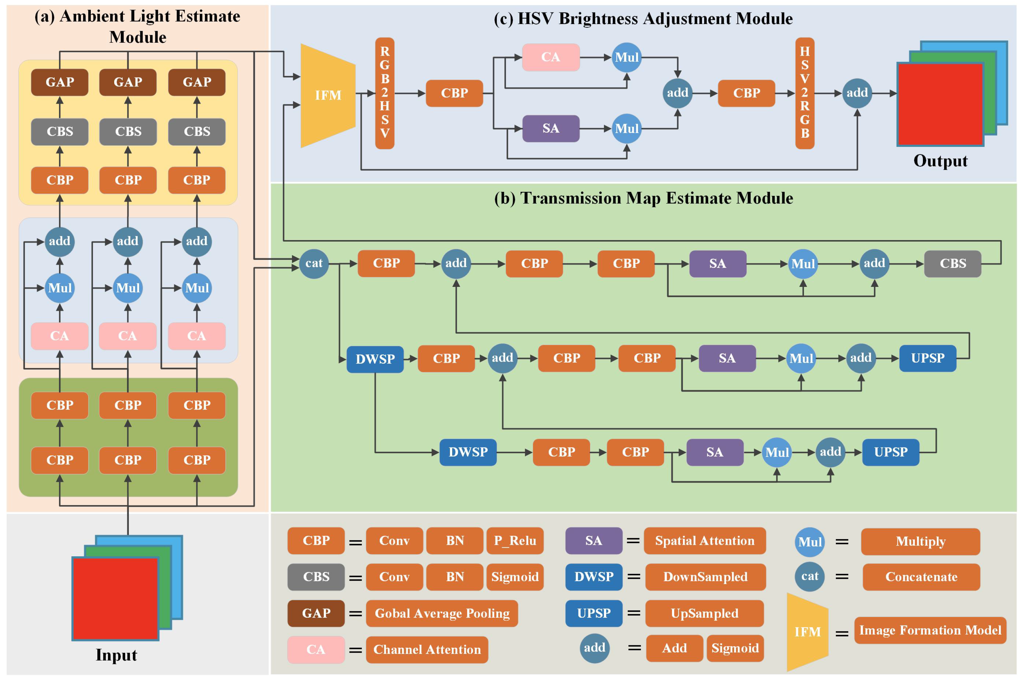
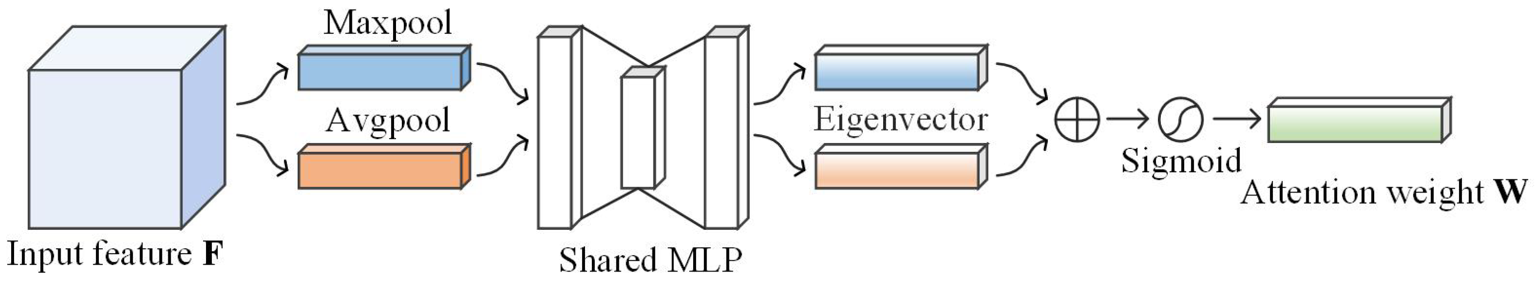
In recent years, scholars have explored underwater image recovery methods using advancements in computer vision technology [3]. He et al. [4] proposed the Dark Channel Prior (DCP) based on the statistical analysis of many natural terrestrial scene images. Then, they used it with an image formation model to estimate the transmission map (TM) and ambient light ($A^c$). The authors achieved adequate image restoration, providing a new approach to solving the image restoration problem. This inspired many DCP-based image restoration methods [5,6]. Given the good results achieved by DCP on natural terrestrial images, many researchers have also applied DCP to underwater image restoration. However, the imaging environments on land and underwater are different, the media are different, and the scattering and refraction laws of light are also different, so it is not good to directly copy DCP for restoration in underwater images. Therefore, researchers have proposed many variants of DCP methods for underwater scenes, such as [7,8,9]. However, the complexity of underwater scenes and artificial lighting effects make many underwater image restoration methods ineffective in recovery. Therefore, an essential component of underwater image restoration is the capacity to precisely estimate the $A^c$ and TM of underwater images.

This paper presents the CABA-Net model for end-to-end underwater image restoration. The proposed approach consists of the following three modules:

• Ambient light ($A^c$) estimation: The ambient light accurate estimation module achieves an accurate estimation of $A^c$ by designing a separate feature extraction network for each color channel and highlighting the most representative features through the channel attention [10] structure so that the network can fully uncover the scene information in the image.
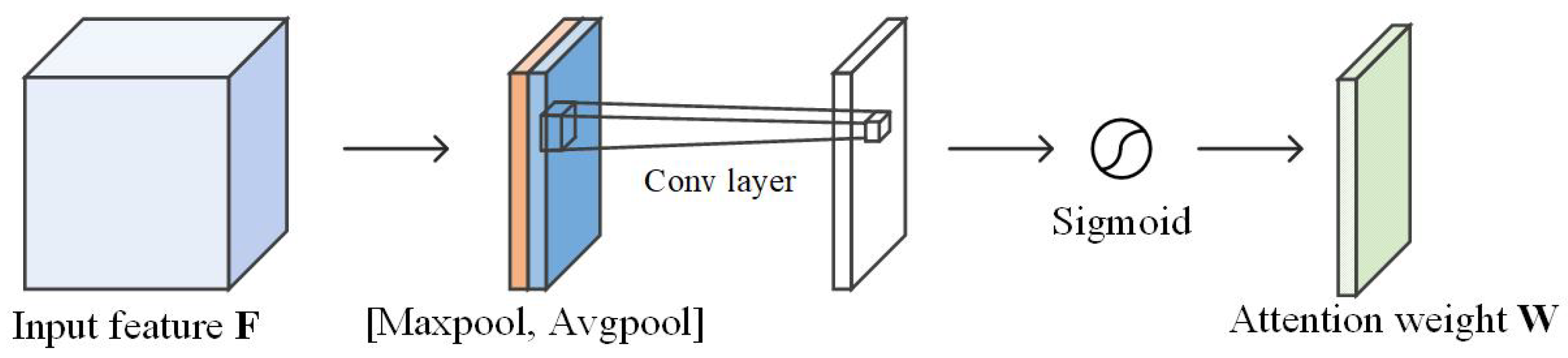
• Transmittance map (TM) estimation: The complexity of underwater scenes was fully considered during the transmittance map estimation. So, in the design of the transmission map estimation module, the spatial attention [10] structure and the coder-decoder structure were combined. The features with rich layers and a global perception field were obtained through convolutional deconvolution and feature fusion operations. Finally, the estimated accurate $A^c$ and accurate TM are substituted into the underwater image formation model to obtain a preliminary recovered underwater image.
• HSV brightness adjustment: The recovered underwater images’ brightness is further adjusted by converting the underwater images to HSV color space and adjusting the brightness of the images.

The major contributions of this study are as follows:

• We present a multi-branch ambient light accurate estimation module that independently applies the convolution module with channel attention mechanism for each color channel, achieving multiple layers combination features, and adaptively selecting the most representative features to precisely estimate the $A^c$.
• We propose an encoder-decoder transmission map estimation module that combines attention structures. Feature extraction of different layers is achieved through a series of downsampled and convolution operations with a spatial attention mechanism. The upsampling and feature fusion operations incorporate different layers of features into a unified structure to estimate the TM accurately.
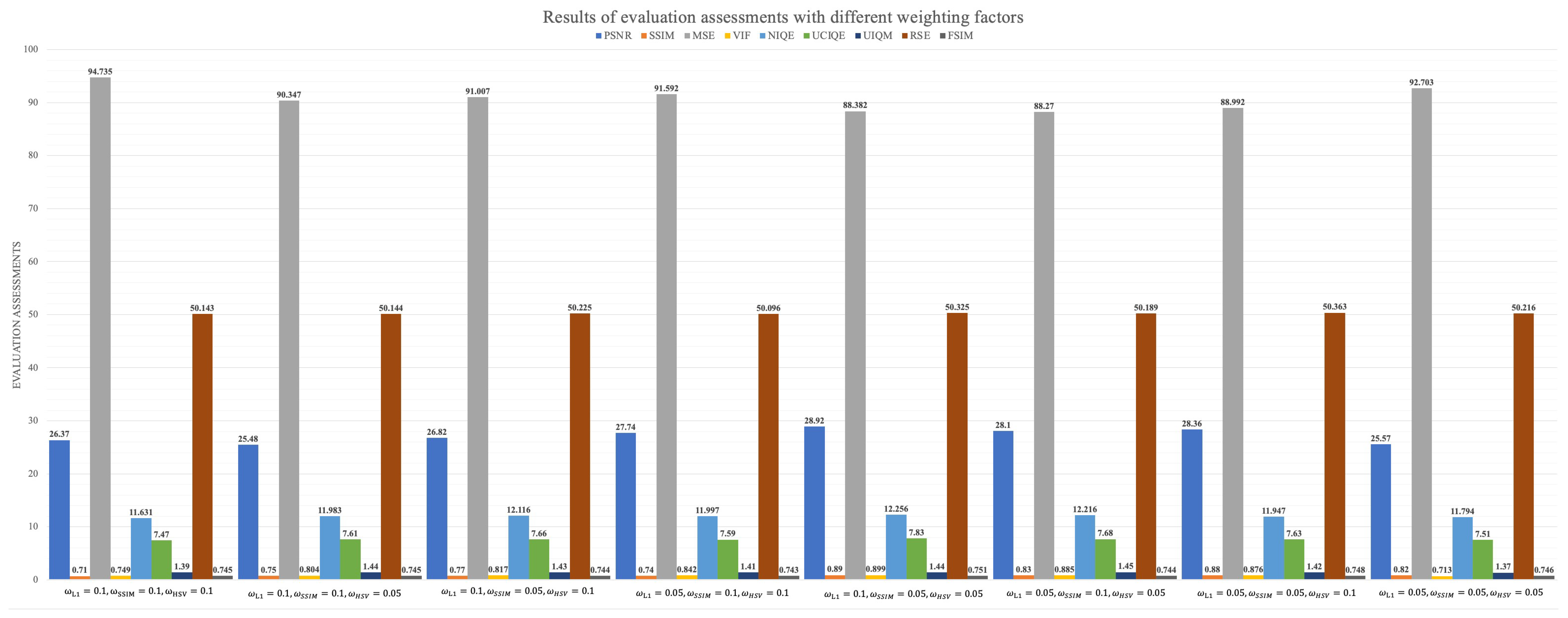
• We introduce a parallel brightness adjustment module combining channel and spatial attention in HSV color space to achieve further image correction. Additionally, we propose a loss function that combines MSE, L1, SSIM, and HSV loss, deriving the optimal weighting coefficients for this function through extensive experimentation.

The remainder of this paper is organized as follows: Section 2 introduces the related works on DCP-based underwater image restoration; Section 3 of the paper discusses the proposed method; Section 4 evaluates and discusses the results; and Section 5 presents the conclusion.

2. Relate Work

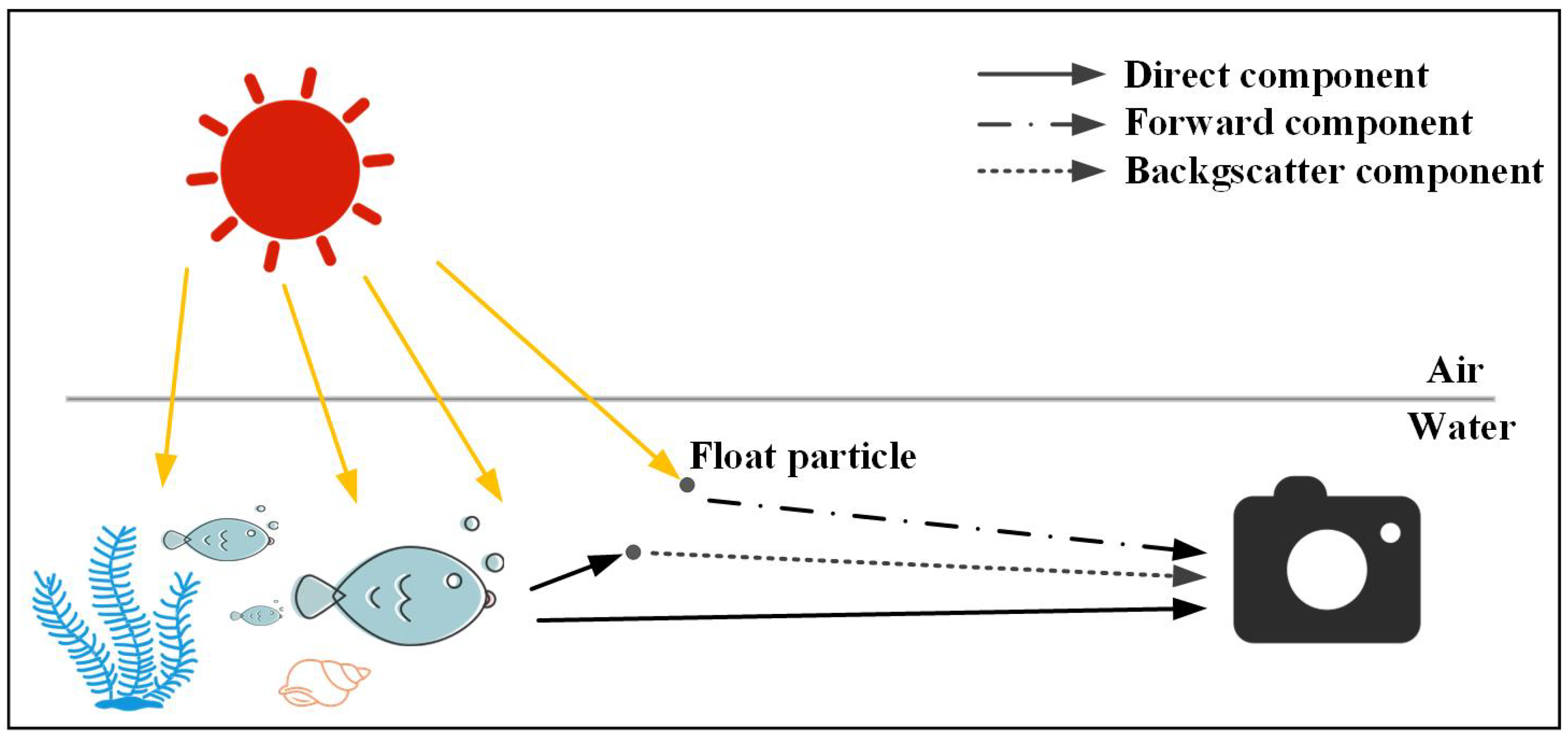
2.1. Underwater Image Formation Model

Light propagation in water is subject to absorption and scattering by water. According to the Jaffe–McGlamery underwater image formation model [11], the underwater image captured by the camera can be regarded as direct component as well as forward and backward-scattered components, as shown in Figure 1.

• The direct component: The reflected light from the scene that reaches the camera after being attenuated during propagation. This represents the underwater image to be recovered.
• The forward component: The part of the light that reaches the camera after small angle scattering during propagation after reflection from the scene surface, which is the leading cause of blurred underwater images. In the underwater shooting process, the camera is close to the subject, and its impact on the process can be negligible.
• The backward scattering component: The portion of the light that reaches the camera just after being scattered by suspended particles. This component is the main contributor to the deterioration of the image contrast.

The following can be used to describe the underwater image formation model:

$$I\left(x\right)=J^c\left(x\right)t^c\left(x\right)+A^c\left(x\right)\left\{1-t^c\left(x\right)\right\},c\in \{r,g,b\}$$

(1)

where $I\left(x\right)$ represents the underwater image, $J^c\left(x\right)$ is the image to be recovered, and $A^c\left(x\right)$ is the ambient light. $t^c\left(x\right)$ is the transmittance at x. The transmittance of the whole image can be formed into TM, indicating the light’s remaining intensity ratio as it reaches the camera after being scattered and absorbed underwater. Each of the red, green, or blue color channels is represented as x.

2.2. Ambient Light Estimation

A crucial component of underwater image restoration is $A^c$. The effectiveness of underwater image restoration is directly related to its precision. The ambient light estimation methods can be divided into DCP ambient light estimation and deep learning methods based on the different principles and characteristics of estimating $A^c$.

Ambient light estimation method based on DCP: Setting the highest luminance pixel in the underwater image as $A^c$ is the simplest method for estimating ambient light [12]. However, $A^c$ is incorrectly estimated in an underwater scene by interferences, such as bubbles and suspended particles. It is unreasonable to estimate $A^c$ from only the perspective of a single pixel. Authors in [13] propose using the brightness value in the image corresponding to the first 0.1% pixels in the dark channel to represent $A^c$. Their approach reduces the effect of suspended particles in the water and improves the robustness of the ambient light estimation algorithm. However, the above method only estimates $A^c$ to a certain extent, disregarding the fact that blue-green light decays much slower than red light in underwater scenes. Drews et al. [14] proposed an accurate estimation of $A^c$ by selecting only the top 0.1% of pixels in the dark blue-green channel as the ambient light estimate. To a certain extent, their approach eliminates the effect caused by the decay of the red-light source. To further accurately estimate $A^c$, Yu et al. [15] accurately estimated $A^c$ by dividing the underwater image into six blocks and selecting flat regions using the pixel variance of each region. Afterward, they applied the DCP method to find the $A^c$ within the selected regions. Additionally, the authors in [16] accurately estimated $A^c$ by fusing the depth-of-field obtained by blurring the red channel and the image. Then, the object and background areas are separated according to the depth-of-field to obtain the ambient light areas. Finally, they selected the top 0.1% brightest pixels in the background as $A^c$. Muniraj et al. [17] proposed a saturation correction factor to adjust for color differences. They then used the correction factor to obtain a precise measurement of $A^c$.

Deep learning method for ambient light estimation: Substantial progress has been made in underwater image ambient light estimation using the recent advancement of deep learning methods for feature extraction. Shin et al. [18] proposed a three-stage cooperative ambient light estimation network with multiscale feature extraction, feature fusion, and nonlinear regression to accurately estimate $A^c$. Peng et al. [19] introduced a method for recovering images affected by scattering and absorption. The approach involves estimating the transmission map by calculating the environmental light differences in the scene and enhancing the degraded image using an image formation model. Subsequently, an adaptive color correction method is employed for color restoration. Woo et al. [20] improves the accuracy of the illuminant chromaticity estimation by leveraging the geometric shape information from specular pixels on object surfaces. The method selects the image path that generates the longest bisector line, leading to more precise illumination chromaticity estimation. Experimental results demonstrate the superiority of this approach in locating illuminant chromaticity compared to state-of-the-art color constancy methods. Cao et al. [21] presented a multiscale structure for estimating the ambient light by stacking filters (size 5 × 5 and 3 × 3), pooling layers (2 × 2), and normalization layers to achieve an accurate estimation of $A^c$. Yang et al. [22] first estimated the depth-of-field map of the underwater image using the whole convolutional residual network. They estimated the red channel ambient light and the attenuation ratio of the RGB color channels using the depth-of-field map. The authors discovered the blue-green channel ambient light according to the attenuation ratio of the RGB color channels and the red channel ambient light to complete the estimation of $A^c$. Wu et al. [23] decomposed the underwater image into high-frequency components (HF) and low-frequency components (LF) to avoid the parameter errors caused by estimating the TM and $A^c$. They used the discrete cosine transform and then transformed them into a two-stage (preliminary enhancement network, refinement network) network to realize the estimation of $A^c$. Fayadh et al. [20] proposed a method for estimating the optimal ambient light in underwater images based on local and global pixel selections. They introduced a block greedy algorithm and a convolutional neural network (CNN) to enhance image dehazing by combining pixel differences and the minimum energy Markov random field (MRF), thereby improving the clarity and color balance performance of underwater images.

2.3. Transmission Map Estimation

The accuracy of the estimated underwater image TM impacts the effectiveness of underwater image restoration. The simplest TM estimates are made directly using the DCP prior derived from the natural terrestrial scenes. However, the restoration effect of DCP methods is ineffective because it does not consider how light diminishes in the water. By analyzing the theory of underwater image formation, Carlevaris–Bianco et al. [24] estimated the TM by calculating the difference between the most significant intensities of the blue-green and red channels. Unfortunately, their restoration effect is not ideal, causing an incorrect estimation of the TM due to the appearance of light-colored areas or artificial light sources in the background region. By analyzing the principle of underwater imaging, Li et al. [25] proposed the Minimum Information Loss Principle (MILP) through the analysis of the underwater imaging principle. Their approach first estimates the red channel transmittance by reducing the information loss of the red channel in the local area. Then, it estimates the blue-green channel transmittance using the ratio relationship of the RGB channel transmittance to accurately estimate the transmittance map. Peng et al. [26] first achieved the estimation of a depth map using gradient information, then estimated the $A^c$ using the scene depth information. Finally, the estimated depth map and $A^c$ were substituted into the image formation model to obtain an accurate TM. Pan et al. [27] proposed a novel method for enhancing underwater images. The approach involves training a convolutional neural network to estimate the transmission map, followed by refining the transmission map using an adaptive bilateral filter. Finally, the output image is transformed into a hybrid domain of the wavelet and directional filter bank for denoising and edge enhancement processing. Based on the analysis of haze-line assumption, Berman et al. [28] proposed a transmittance estimation method centered on the ratio between RGB channel attenuation factors. They achieved the accuracy of underwater image transmittance map estimation. However, most pixels will point in the same direction when the $A^c$ brightness is significantly greater than the scene, making it difficult to detect the haze line. Underwater red light attenuates at a rate that is noticeably higher than green-blue light because of the difference between underwater and natural terrestrial scene images. Song et al. [29] show that ${\mathrm{J}}_{\mathrm{dark}}^{\mathrm{rgb}}=0.1$ is more consistent with the underwater image situation based on many underwater image statistics. Therefore, they used ${\mathrm{J}}_{\mathrm{dark}}^{\mathrm{rgb}}=0.1$ to replace the DCP prior and combined ${\mathrm{J}}_{\mathrm{dark}}^{\mathrm{rgb}}=0.1$ with the underwater image formulation model to accurately estimate the TM. Zhou et al. [30] has developed a dehazing method for underwater images under different water quality conditions, utilizing a revised underwater image formation model. The method relies on a scene depth map and a color correction approach to mitigate color distortions. Firstly, a method for estimating the depth of underwater images is designed to create a transmission map. Subsequently, based on the revised model and the estimated transmission rates, the method estimates and removes backscatter. Liu et al. [31] addresses the restoration and color correction issues of underwater optical images through an improved adaptive transmission fusion method. The approach involves applying a modified reverse saturation map technique to enhance the transmission map. Additionally, a novel underwater light attenuation prior method is introduced. Li et al. [32] proposes a method for estimating the transmission map of underwater images. The approach enhances contrast through grayscale quantization, utilizes Retinex color constancy to eliminate lighting and color distortion, establishes a dual-transmission underwater imaging model to estimate background light, backscatter, and direct component transmission. Dehazed images are then generated through an inversion process.

3. Proposed Method

By analyzing the image formation model, we design an end-to-end network named CABA-Net to accurately estimate $A^c$ and TM in underwater image restoration methods, utilizing a combination of attention mechanisms and brightness adjustments. Also, we introduce a brightness adjustment module of the HSV color model to further improve the hue and luminosity of the recovered image. The network framework structure is illustrated in Figure 2. Firstly, the original underwater image is fed into the module for a precise ambient light estimation to estimate the accuracy of $A^c$. Then, the original underwater image is concatenated with the accurate $A^c$ and passed through the TM accurate estimation module to derive an accurate TM. Finally, the underwater image is restored by substituting the estimated $A^c$ and TM into the image formation model. However, issues like poor contrast and dim brightness in some scenes remain in the corrected underwater images. Therefore, we also introduce an HSV luminance adjustment module combining the spatial and channel attention mechanisms to complete the stretching of the scene contrast and luminance.

3.1. Ambient Light Estimate Module

Figure 2a shows the details of the ambient light accurate estimation module that achieves accurate RGB ambient light estimation. This is achieved by designing three independent ambient light estimation branches for the input underwater image. Each branch is further divided into three steps: shallow feature extraction, deep feature extraction combined with channel attention mechanism, and feature fusion. First, two CBP modules are used for shallow feature extraction: the input image is convolved with a step size of 1, a size of 3 × 3, and 12 kernels. Then convolution outputs are batch-normalized to lessen the effect of changes in the network data distribution on the model parameter training. Finally, the nonlinearization of the normalized results using the P_ReLU activation function is used to complete the extraction of shallow features from the input image. Relying on shallow feature extraction modules may accurately estimate $A^c$ in simple scenes. Still, it is powerless in complex scenes. This study also introduces a channel attention mechanism based on shallow features to enhance the precision and reliability of the estimation ambient light method, enabling the network to further mine deeper features from shallow features. Channel attention is first aggregated in the network using a maximum and global average pooling to provide two feature weight matrices. Then, the two weight matrices are input to a shared multilayer perceptron to generate a more representative eigenvector. After that, the two eigenvectors are added together, and the Sigmoid function is applied to obtain the final channel attention weight. Finally, deep feature extraction is achieved by multiplying the feature map by the final channel attention weight. The shallow features and deep features are combined in feature fusion to combine the multiple levels of features passing through the CBP, CBS modules, and the GAP model, completing an accurate estimation of $A^c$.

Channel attention: For a given multi-channel feature map $F\in R^{C\times H\times W}$, there is a difference in the information depicted in each channel’s feature map. Channel attention generates a weight matrix $W\in R^{C\times 1\times 1}$, which is subsequently multiplied by the inputs. This way, the network concentrates on the more relevant channel information and extracts accurate and efficient valuable features. The structure of the channel attention is illustrated in Figure 3.

3.2. Transmission Map Estimate Module

The TM is the proportion of the underwater light source remaining at the camera after scattering and absorption. According to the Jaffe–McGlamery model of underwater image formation, the TM encapsulates significant scene information and water conditions. Therefore, the key to TM estimation is to extract more scene information and water conditions in a complex scene with a large number of color-cast underwater images. The traditional method can extract more features by increasing the depth of the convolutional neural network. Unfortunately, the features suffer from decay and gradient disappearance as the network layer deepens, resulting in the loss of the extracted features’ middle and low-layer details; the recovery effect is inefficient. Therefore, we discard the previous approach of using deeper convolutional neural networks for TM estimation. Instead, we use an encoder–decoder structure to reduce the problem of feature loss between high-level and low-level features. In addition, we introduce a spatial attention structure with complete spatial information, focusing on the capability to purposefully allow the estimated TM to retain more spatial location information and highlight certain key regions of the image to achieve better TM estimation. The encoder-decoder module, combined with the attention structure, consists mainly of three parts, as follows:

• Encoder module: The underwater image and $A^c$ are first concentrated. Two downsamples are performed to obtain three levels of feature representation. The output obtained from each downsample is subjected to two simple feature extractions to complete the extraction of preliminary features.
• Deep feature extraction combining spatial attention mechanism module: The preliminary extracted features are first subjected to maximum and global average pooling, generating two feature descriptors for each spatial location. Then, the two feature descriptors are superimposed, and a 7 × 7 size convolution kernel and Sigmoid function are used to generate a spatial attention map. Finally, the spatial attention map is multiplied with the preliminary feature map to complete the extraction of essential information and detailed features of underwater images.
• Decoder module: The extracted deep features are upsampled and expanded to the same size as the previous level features. Then, they are subjected to a feature extraction of the previous level combined with the spatial attention mechanism to integrate features from different levels.

The above steps were repeated twice to estimate a TM incorporating different layers of features to accurately estimate the TM.

Spatial attention: Spatial attention is more focused on the spatial location information of features than channel attention. It learns the two-dimensional spatial weights $W\in R^{1\times \mathrm{H}\times \mathrm{W}}$ by using the relationship between different spatial locations and then multiplying them with the input features to direct the network to focus more on the essential aspects of the spatial locations of the features. Figure 4 shows the structure of spatial attention.

3.3. HSV Brightness Adjustment Module

HSV (Hue, Saturation, and Value) is a color representation model that characterizes colors based on three components: hue, which represents the type of color; saturation, indicating the intensity or vividness of the color; and value, determining the brightness or lightness of the color. Compared to the RGB color model, HSV separates color attributes, making it easier for users to understand and adjust different aspects of color. In the context of underwater image processing, leveraging the HSV color space provides a more intuitive and effective way to manipulate color attributes.

The estimated accurate $A^c$ and TM introduced in the image formation model achieves an effective correction of blurring and color-cast underwater images. However, the corrected underwater images still suffer from insufficient contrast and darkness in some scenes. Therefore, we enhance scene brightness by converting the recovered underwater image from the RGB to HSV color space and then adjusting its brightness with a parallel channel and pixel attention. The corrected underwater image is first applied to the HSV color space by applying the rgb2hsv formula. Then, the channel attention is applied to the image under the HSV color space to obtain the different layer features in the underwater image. Similarly, spatial attention was also used in HSV color space images to brighten darker pixels and inhibit overexposed pixels. Finally, the features extracted by spatial and channel attention are fused by a 1 × 1 convolution. The hsv2rgb formula is applied to convert the image into a RGB color space to complete the image’s contrast and brightness enhancement.

3.4. Loss Function

This study ensures that CABA-Net can generate images with sound and visual effects, since the most common loss functions no longer accurately reflect the degree of optimization of the image in all aspects. Therefore, we made the output image more closely resemble the actual image by combining L1 loss, MSE loss, SSIM loss, and HSV loss in a weighted combination, where $I_i$ is defined as the predicted image and ${\widehat{I}}_i$ is the precise ground truth image. The following equation depicts the total loss function:

$$L={\omega }_{L1}·L_{L1}+{\omega }_{MSE}·L_{MSE}+{\omega }_{SSIM}·L_{SSIM}+{\omega }_{HSV}·L_{HSV}$$

(2)

where $L_{L1}$, $L_{MSE}$ and $L_{SSIM}$ are the RGB color space loss function, and $L_{HSV}$ is the HSV color space function. These functions and terms are defined in more detail below.

MSE loss ($L_{MSE}$): MSE loss is a common loss function in computer vision tasks. It performs well in image content enhancement. It can be expressed as the squared difference between the clear ground truth images and the predictions:

$$L_{MSE}={({\widehat{I}}_i-I_i)}^2$$

(3)

L1 loss ($L_{L1}$): Adopting MSE loss as the loss function could obtain a good enhancement effect to recover the image, but it will amplify the loss between the maximum and minimum errors. Therefore, we introduced L1 loss to alleviate the outlier sensitivity problem introduced by the MSE loss. In addition, L1 loss produces less noise than MSE loss, leading to a better restoration of darker regions. The following equation depicts $L_{L1}$:

$$L_{L1}={∥{\widehat{I}}_i-I_i∥}_1$$

(4)

SSIM loss ($L_{SSIM}$): The introduction of L1 loss has many benefits, but it can also lead to problems such as blurring in the generated images. For this reason, the structural similarity loss function is also introduced for enhancing texture and structural features to alleviate the blurring problem caused by L1 loss. We first transform the RGB image to a grayscale image and then compute the SSIM value for each pixel using an 11 × 11 image block. The following equation depicts the SSIM value:

$$SSIM\left(x\right)=\frac{2{\mu }_I\left(x\right){\mu }_{\widehat{I}}\left(x\right)+c_1}{{\mu }_I^2\left(x\right)+{\mu }_{\widehat{I}}^2\left(x\right)+c_1}·\frac{2{\sigma }_{I\widehat{I}}\left(x\right)+c_2}{{\sigma }_I^2\left(x\right)+{\sigma }_{\widehat{I}}^2\left(x\right)+c_2}$$

(5)

where ${\mu }_{\widehat{I}}\left(x\right)$ and ${\mu }_I\left(x\right)$ represent the means of the pixels in the predicted and clear ground truth images. Similarly, ${\sigma }_{\widehat{I}}\left(x\right)$ and ${\sigma }_I\left(x\right)$ are the variances of the pixels in the predicted and clear ground truth images. ${\sigma }_{I\widehat{I}}\left(x\right)$ denotes the cross-covariance. c1 is set to 0.02 and c2 to 0.03 [33]. The following equation depicts the SSIM loss:

$$L_{SSIM}=1-\frac{1}{N}\sum _{i=1}^{N}SSIM\left(x_i\right)$$

(6)

HSV loss ($L_{HSV}$): The HSV brightness adjustment module in the CABA-Net network does the brightness adjustment in the HSV color space; thus, it is not enough to only introduce the loss function in the RGB color space. Therefore, we introduce the HSV loss to adjust the hue and luminosity of the recovered image. The following equation depicts the HSV loss:

$$L_{HSV}={∥{\widehat{S}}_i{\widehat{V}}_{i}cos\left({\widehat{H}}_i\right)-S_i{V}_{i}cos\left(H_i\right)∥}_1$$

(7)

where ${\widehat{H}}_i$ and $H_i$ are the predicted and clear ground truth image hue, which are taken in the range between $[0,2\pi )$. ${\widehat{S}}_i$ and $S_i$ are the predicted and clear ground truth image saturations, taken in the range $[0,1]$. ${\widehat{V}}_i$ and $V_i$ are the predicted and ground truth image values, respectively, taken in the range $[0,1]$.

Loss term weights: Based on the gathered literature, it is evident that MSE loss plays a predominant role in the restoration of underwater scenes. Therefore, in selecting parameters, we followed the parameter allocation methods outlined in references [34,35,36]. Specifically, we assigned a substantial weight to MSE, setting it at 0.8. We then explored various combinations of weights for SSIM, L1, and HSV, considering values of 0.1 and 0.05. Through a series of experimental comparisons, we obtained PSNR, SSIM, MSE, VIF, NIOE, UCIOE, UIOM, RSE, and FSIM indices for each scenario. The results, depicted in the accompanying Figure 5, guided our selection of the optimal weight coefficients for evaluation metrics (i.e., L1 = 0.1, SSIM = 0.5, HSV = 0.05), as our optimal parameters with a thorough comparison.

4. Experimental Results

This study compares underwater image enhancement methods, traditional underwater image restoration, and deep learning for underwater image restoration methods, and underwater image enhancement methods on two datasets of real underwater scenes to assess the efficacy of the approach. Underwater image enhancement methods compared include Histogram Equalization (HE) [37], Multiscale Fusion (MulFusion) [38], and Wavelet-Based Dual-Stream (WBDS) [39]. Traditional underwater image restoration methods include Underwater Dark Channel Prior (UDCP) [14], Image Blurriness and Light Absorption (IBLA) [26], and Dual-Background Light adaptive fusion and Transmission Map (DBLTM) [40]. Meanwhile, the deep-learning underwater image restoration methods include Combining Deep Learning and Image Formation Model (DLIFM) [41] and Learning Attention Network (LANet) [42]. This section presents the network training details and performs a series of qualitative visual comparisons in different scenes, followed by objective quantitative comparisons. Finally, we performed several ablation experiments to validate each element of CABA-Net and the loss functions.

4.1. Network Training Details

This study randomly chose 800 pairs of underwater images from the UIEB [43] to train the CABA-Net. The training covers diverse underwater environments, various types of underwater quality deterioration images, and a vast array of underwater image content. However, there are still not enough underwater images to train the CABA-Net. Therefore, we included 200 pairs of synthetic underwater images from the dataset in [44]. Both (1000 in total) were used to train the CABA-Net. The input image was neither resized nor randomly cropped to make the proposed network closer to the actual situation. We use the Adam optimizer on Inter(R) i5-6500Q CPU, 16GB RAM, and an Nvidia GTX 3090 GPU with a batch size of 1 across 500 epochs to train the model.

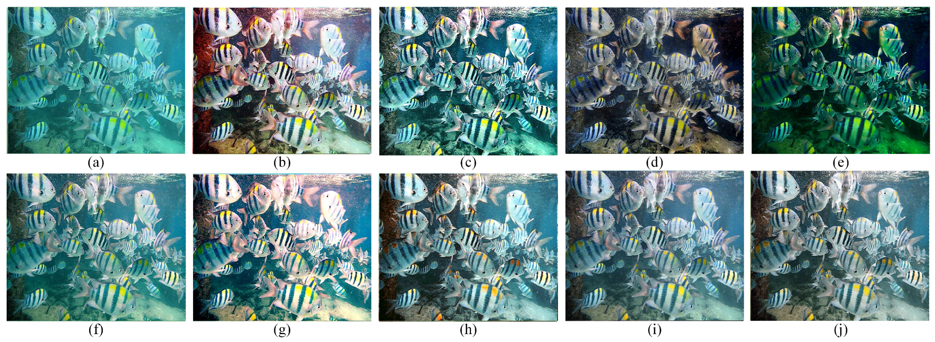
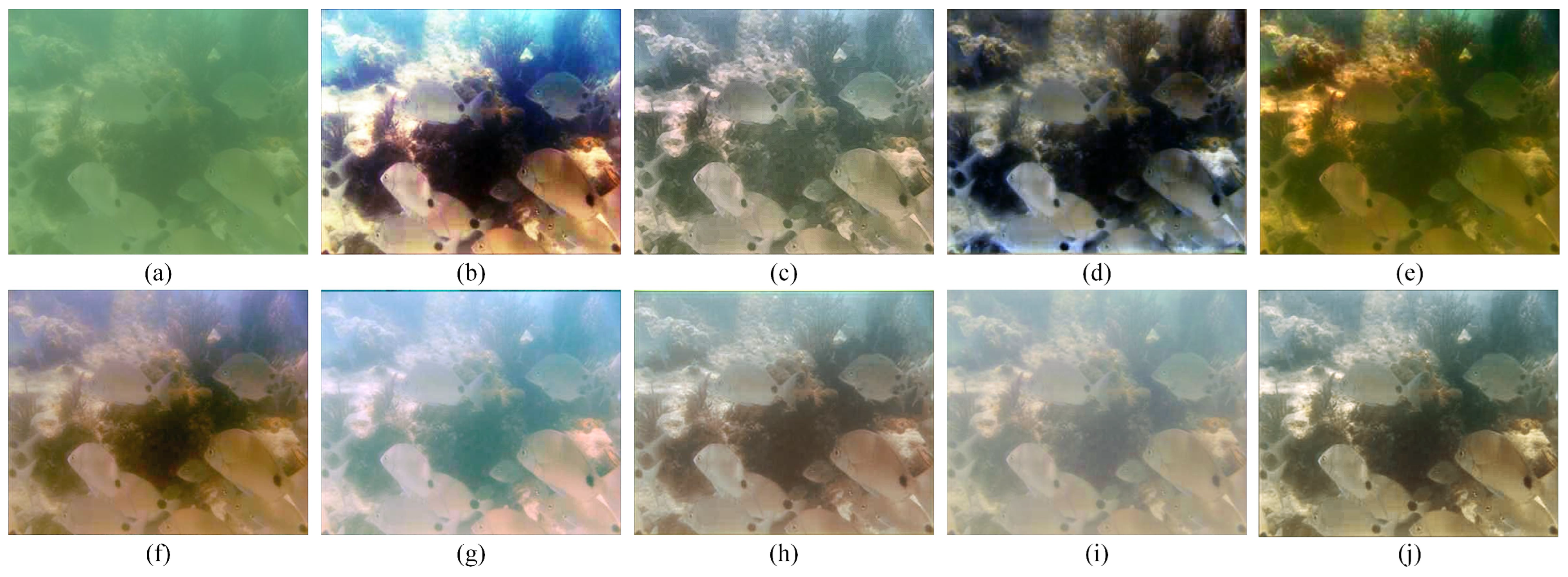
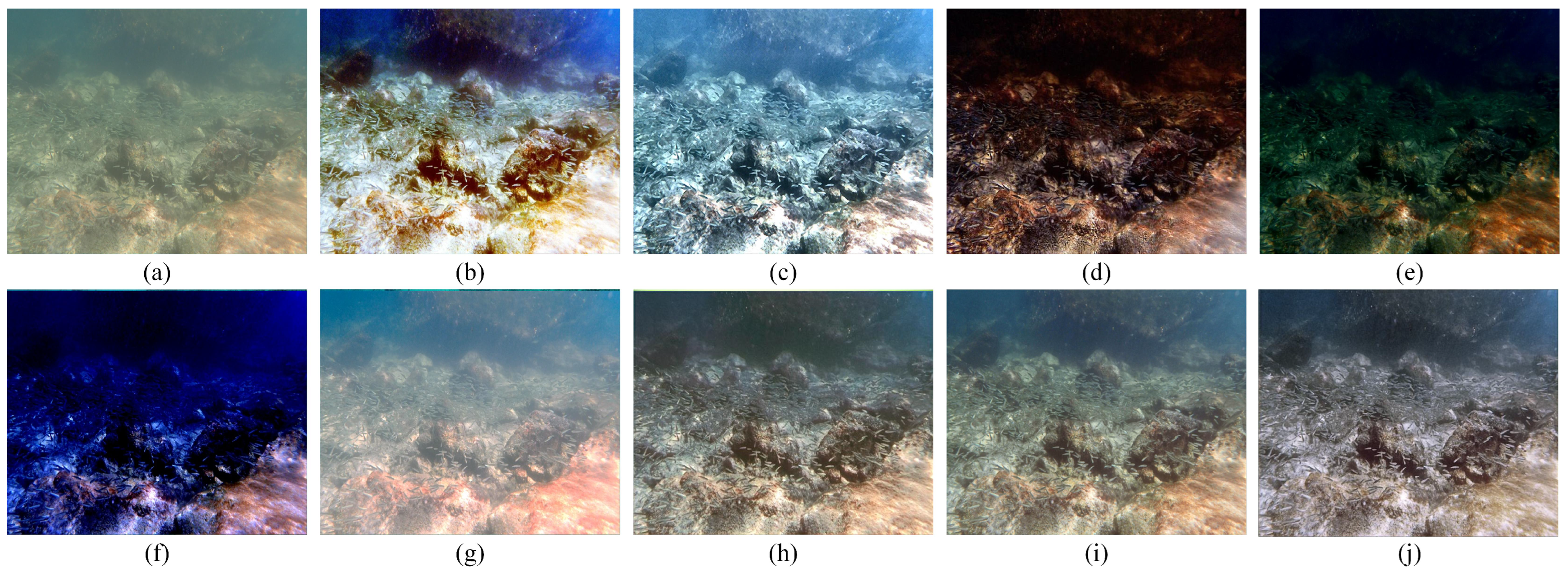
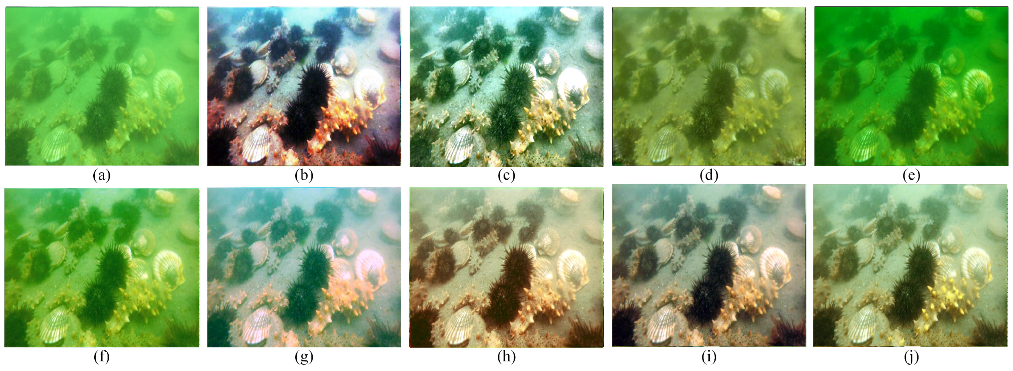
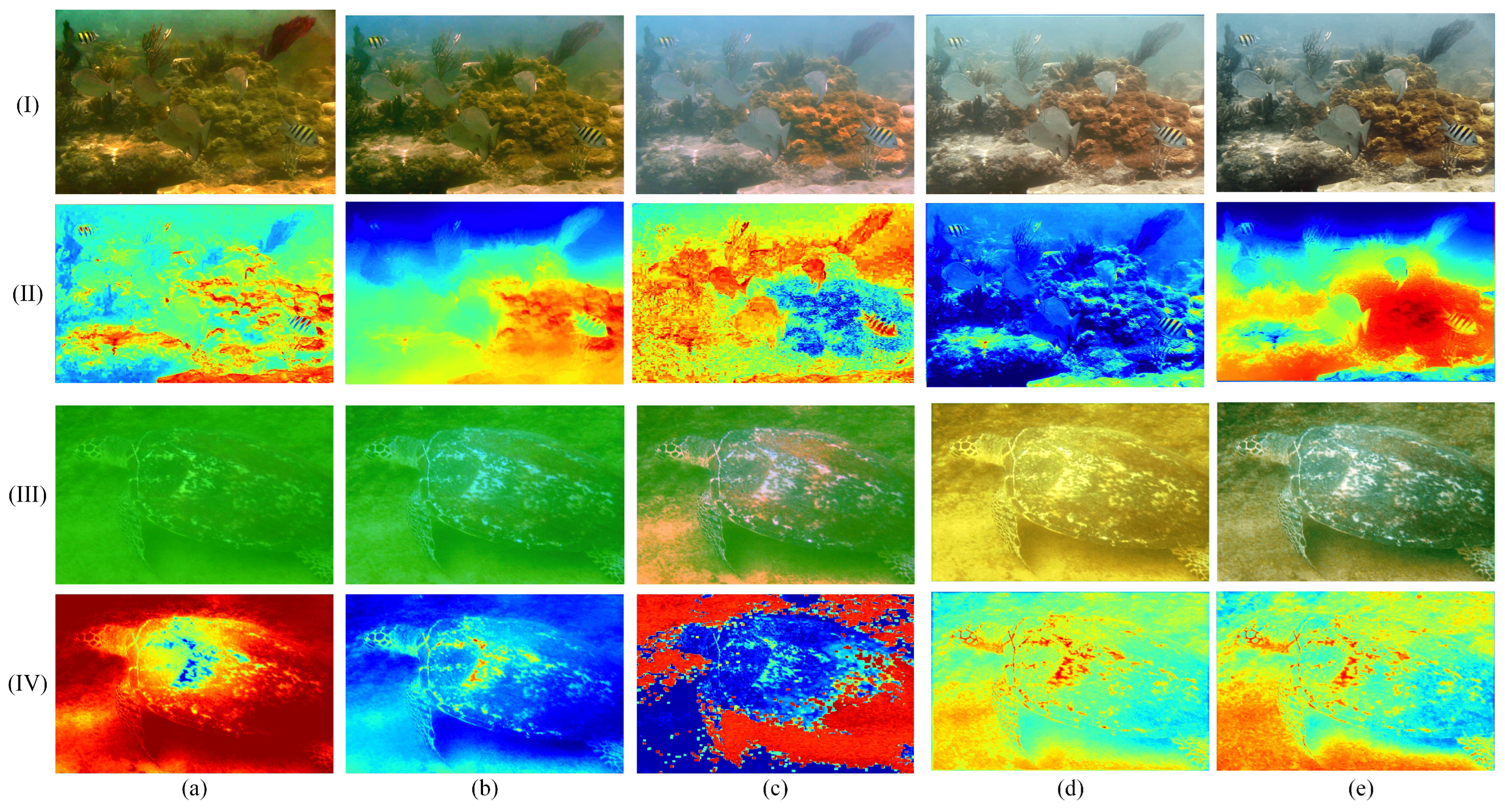
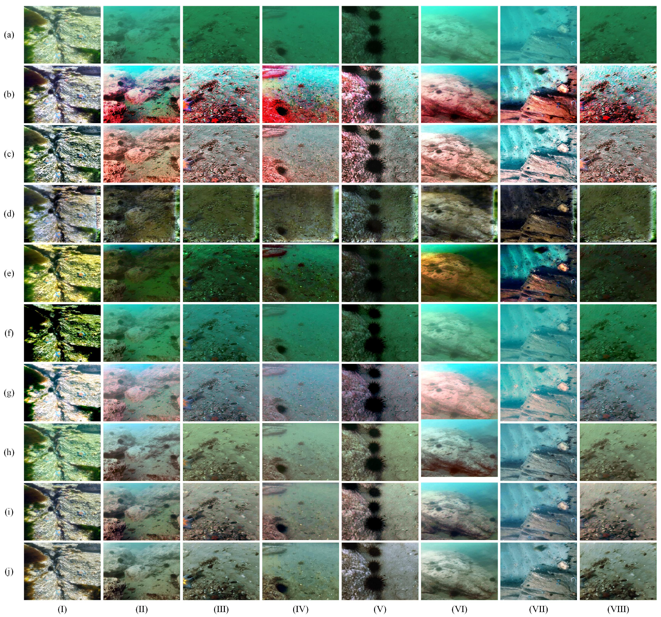
4.2. Subjective Evaluation

Figure 6, Figure 7, Figure 8 and Figure 9 show the comparative results of image restoration between the proposed method and other comparison methods. They can represent near, medium, far, and complex underwater scenes. From Figure 6b, Figure 7b, Figure 8b and Figure 9b, the luminance of the underwater image is enhanced the most, despite the HE method. Still, some scenes of the image process have problems such as the overexposure and reddishness of the subject: the recovery effect is inefficient. Figure 6c, Figure 7c, Figure 8c and Figure 9c, obtained by the MulFusion method, remove the blue and greenish of underwater images to a certain extent. However, the scene-related information is missing in the recovery process. The recovered images will have problems of redness and excessive scene sharpness. The WBDS method uses a wavelet decomposition processing and fusion to achieve underwater image recovery. However, the method does not only improve the image brightness but also degrades the quality of the images, indicating that the method does not apply to underwater image recovery, as shown in Figure 6d, Figure 7d, Figure 8d and Figure 9d. Figure 6e, Figure 7e, Figure 8e and Figure 9e show that the image’s brightness processed with the UDCP method does not increase, and the color distortion is severe: the restoration effect is inefficient, indicating that the restoration method derived from natural terrestrial scenes combined with the underwater image formation model does not apply to underwater image restoration. The restoration effect of Figure 6f, Figure 7f, Figure 8f and Figure 9f processed by the IBLA method is not apparent, and the image contrast of some scenes is reduced due to the inability to reasonably estimate the TM. The images processed by the DBLTM method using NUDCP before being combined with fused $A^c$ were corrected in brightness and color reproduction. However, there is a color cast in the restoration image in some scenes: the restoration effect is not apparent. To some extent, the underwater image processed by the DLIFM method solves the problem of a blue and greenish underwater image. However, the method uses a simple estimation of the $A^c$ and TM, which cannot properly recover the underwater image in complex scenes, as shown in Figure 9h. The recovered image with the LANet method has a higher color reproduction and a better recovery effect. However, the subject in some scenes will also have the phenomenon of tonal reddening: the recovery effect is still not ideal. In comparison, the proposed method solves the problem of subject color-casting in DBLTM and LANet methods. It improves the image’s luminance to a great extent while maintaining the original color of the image, allowing the corrected underwater image to maintain the most natural tones.

The quality of the restored image is based on how well the $A^c$ and TM was obtained throughout the restoration procedure. A further comparative experiment is carried out to compare the estimation of $A^c$ and TM by different methods. This section compares only the remaining four methods, since HE, MulFusion, WBDS, and LANet methods do not require estimating TM and $A^c$. The results are shown in Figure 10. Among the four methods compared, the $A^c$ estimated by the proposed method has the lowest pixel intensity, lower than the $A^c$ of UDCP, IBLA, DBLTM, and DLIFM. In addition, due to erroneous $A^c$ estimation, the foreground and background were wrongly reversed in the UDCP method, decreasing the image’s luminance after enhancement. The IBLA method overestimates the TM, and the recovery is inefficient. The DBLTM method can accurately estimate the $A^c$ in simple scenes. However, they are useless in complex scenes, such as Figure 10c(IV). The DLIMF can estimate a better TM, but the detailed outline estimation of the scene subject is still not accurate enough. The transmission image obtained using the proposed method has more foreground and background layers than the TM obtained from the other four methods. The proposed method can discern the background and foreground sections of the turtle and shipwreck images with precision. Furthermore, the method significantly enhances the hue and luminance of the recovered underwater image, demonstrating the potency of underwater image restoration.

4.3. Objective Assessment

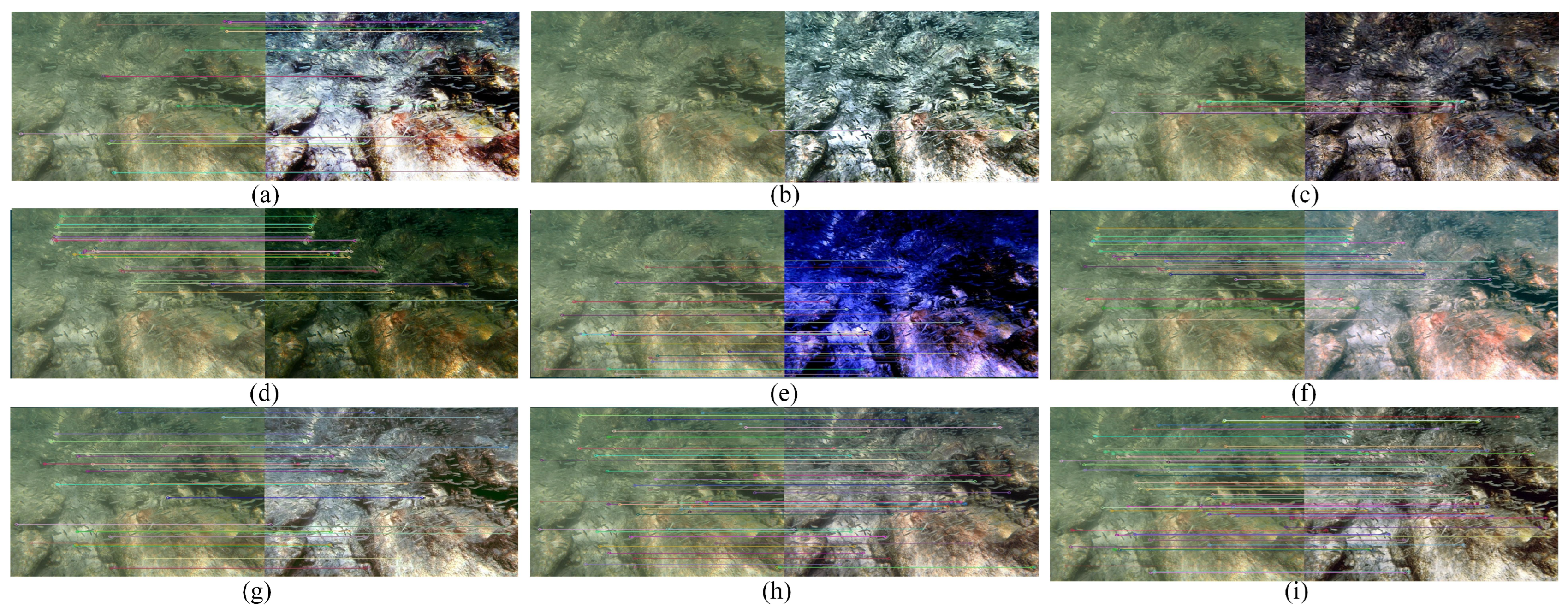
We compare the objective evaluation of the recovered images acquired with other underwater image recovery methods to demonstrate the efficacy of the proposed method. There are two types of objective assessment, depending on the availability of a reference image: full-reference image quality assessment (FR) and no-reference image quality assessment (NR).

FR assessments requires the recovered image to have a corresponding actual reference image to calculate the approximation. Commonly used FR metrics include:

Peak Signal-to-Noise Ratio (PSNR) [45]: PSNR measures the ratio of the maximum possible power of a signal to the power of corrupting noise. Higher PSNR values indicate less noise and better image quality.

Structural Similarity Index Metric (SSIM)s [46]: SSIM compares the structural similarity between the recovered image and the reference image. A higher SSIM value suggests a better preservation of the structural detail.

Mean Squared Error (MSE) [47]: MSE quantifies the average squared difference between corresponding pixel values in the recovered and reference images. Lower MSE values indicate better image similarity. In [48], the performance of the image fusion model is evaluated using MSE.

Visual Information Fidelity (VIF) [49]: VIF evaluates the fidelity of visual information in the recovered image compared to the reference image. VIF is commonly used to compare the performance of image processing algorithms, such as image denoising, image enhancement, or image compression.

Feature Similarity Index Metric (FSIM) [50]: FSIM assesses the similarity of structural features between the recovered and reference images, taking into account luminance, contrast, and structure, and providing a holistic measure of image quality. Higher FSIM values signify better feature preservation.

Subjective Quality Assessment (SRE) [51]: SRE involves obtaining subjective evaluations from human observers to assess the perceived quality of reconstructed or enhanced images. It provides a perceptually relevant evaluation, capturing aspects that quantitative metrics may not fully address. SRE is essential for understanding how well algorithms align with human perception and is commonly used in image processing research to gauge the overall visual impact of techniques.

NR directly calculates the restoration image’s color, contrast, and saturation and integrates them into an overall image assessment to represent the underwater image quality. Commonly used NR metrics include:

Underwater Color Image Quality Evaluation (UCIQE) [52]: UCIQE assesses the color quality of underwater images. Higher UCIQE values indicate better color reproduction.

Underwater Image Quality Measure (UIQM) [53]: UIQM provides a comprehensive evaluation of overall image quality, considering factors like contrast and brightness. Higher UIQM values represent better image quality.

Natural Image Quality Evaluator (NIQE) [54]: NIQE measures the naturalness of the restored image. Lower NIQE values indicate more natural-looking images.

The metrics PSNR and MSE are regarded as conventional measures of image quality among those mentioned above. However, it is worth noting that they are relative metrics and may lack sensitivity to changes imperceptible to the human eye [55]. In contrast, structural metrics such as SSIM and FSIM are more adept at simulating the human perception of image quality. Additionally, we considered VIF to provide a more comprehensive assessment of visual information fidelity in the images. After careful consideration, we selected a set of nine metrics, including PSNR, SSIM, MSE, VIF, RSE, FSIM, NIOE, UCIOE, and UIOM, to evaluate our model. Through these metrics, we gain a more comprehensive understanding of our method’s performance across various aspects.

The UIEB dataset served as the complete quality assessment of the FR evaluation because there is no reference image for underwater images in the RUIE dataset.

Table 1. The average PSNR, SSIM, MSE, VIF, FSIM, SRE, NIQE, UCIQE, and UIQM on the dataset UIEB for various images for each method and average processing time per image of algorithms.

	Full-Reference Quality Assessment						No-Reference Quality Assessment			Average Processing Time per Image of Algorithms
	PSNR	SSIM	MSE	VIF	FSIM	SRE	NIQE	UCIQE	UIQM
HE	28.203	0.751	98.577	0.809	0.74	49.883	12.41	7.018	1.352	0.08 s
MulFusion	28.09	0.672	101.19	0.816	0.729	49.963	12.505	5.676	1.424	1.14 s
WBDS	28.59	0.61	104.447	0.641	0.695	49.441	15.128	5.648	0.883	3.59 s
UDCP	27.869	0.507	106.409	0.798	0.674	50.148	13.903	7.586	0.418	35.50 s
IBLA	28.127	0.566	100.921	0.741	0.728	47.221	13.253	2.231	0.316	91.29 s
DBLTM	28.074	0.755	102.131	0.81	0.703	50.068	13.95	4.978	1.118	61.36 s
DLIFM	28.627	0.846	90.19	0.822	0.73	47.545	15.681	4.166	1.039	0.51 s
LANet	28.792	0.89	89.459	0.819	0.747	50.883	13.936	4.21	0.912	3.56 s
Our	28.92	0.827	88.382	0.899	0.751	50.325	12.256	7.83	1.44	0.56 s

shows the average scores for the full-reference image quality assessment (PSNR, SSIM, MSE, VIF, FSIM, and SRE). The values of the no-reference image quality assessment (UCIQE, UIQM, and NIQE) during the NR evaluation were calculated using the underwater images of the RUIE and UIEB dataset, as presented in Table 1.

Table 1 demonstrates that our proposed method achieves SSIM and SRE values consistently above 0.8 and 50, respectively. Moreover, compared to the suboptimal LANet, our method shows improvements of 0.44%, 1.2%, 9.76%, and 5.35% in PSNR, MSE, VIF, and FSIM values, respectively. Additionally, concerning image brightness, detail enhancement, and visual perception, our proposed method restores underwater images closer to the original, significantly enhancing image clarity and eliminating blurring effects compared to other methods. For NR, our method outperforms the suboptimal HE, with NIQE and UCIQE increasing by 1.24% and 11.5%, respectively, and UIQM improving by 1.12% compared to the suboptimal MulFusion. This indicates a significant enhancement in the tone and brightness of underwater images achieved by our proposed method. Furthermore, we conducted experiments to compare the processing time required by different methods. The images used in this comparison had a size of 870 × 1230. The last column of Table 1 represents the average processing time for each algorithm per image. Compared to other traditional methods, our approach ranks just below the He image enhancement method. In contrast, among deep learning methods, it falls significantly below DBLTM and LANet. It closely competes with the DLIFM method, showcasing a minimal difference. Therefore, our approach demonstrates a considerable advantage in terms of restoration speed.

4.4. Application

The further effectiveness of the method was analyzed in terms of local feature point matching and test results on a new dataset to demonstrate its efficacy and universal applicability.

Local feature points matching: Local feature points matching is an essential visual perception task, which is the foundation of photogrammetry, 3D reconstruction, and image stitching. The quantity of local feature points is strongly connected with image quality, indicating the degree of detail in the corrected underwater image. This paper uses the original implementation of SIFT to calculate keypoint points, as shown in Figure 11. Among the eight methods compared, the recovered underwater image of this study has the best recovery effect and detects the most significant number of feature points, convincing evidence that our method is effective.

Robustness test: Several subjective evaluations were also conducted in the RUIE [41] dataset to further illustrate the efficacy and robustness of the method. Many underwater images from real ocean sceneries are included in the RUIE. These images can be separated into the UIQS and UCCS based on the disparity between image visibility and color cast. The UIQS can be divided into five levels (A, B, C, D, and E) based on the difference in the UCIQE value. The UCCS is separated into three levels based on the different values of blue channels in the CIElab color space: bluish, greenish, and blue-green. This study randomly selected five levels of images from the UIQS (Figure 11a) and three levels of images from the UCCS (Figure 11a. The results of the subjective evaluations are shown in Figure 12(I–VIII).

From Figure 12(I–V), our method could demonstrate a good recovery effect in the face of five distinct levels of images from the Underwater Image Quality Set of A–E. It removes the blurring effect and addresses the underwater image’s color-cast problem. From Figure 12(VI–VIII), it is evident that our method can successfully correct the color-cast in all three color-biased underwater images from the Underwater Color Cast Set, not only recovering the blue-biased and green-biased underwater images to their original colors but also not causing the reddish phenomenon in the underwater subjects. The proposed method has the best recovery effect and robustness among the eight underwater image recovery methods.

4.5. Ablation Study

We conducted a network and loss function ablation study to demonstrate that the proposed method produces the best underwater image recovery results when the three network and loss function modules act simultaneously.

Network Ablation Study: To determine the effect that each network component module has on the results, an ablation analysis is performed on the ambient light module (w/o BK Model), transmission map module (w/o TM Model), and HSV brightness adjustment module (w/o HSV Model). A simple convolution module is used to replace the feature extraction module proposed in this paper in each ablation study for a comparative study. The network ablation experiment results for objective quality are displayed in

Table 2. The average PSNR, SSIM, MSE, VIF, FSIM, SRE, NIQE, UCIQE, and UIQM values using all modules and after removing any one module.

	Full-Reference Quality Assessment						No-Reference Quality Assessment
	PSNR	SSIM	MSE	VIF	FSIM	SRE	NIQE	UCIQE	UIQM
Full Model	28.92	0.827	88.382	0.899	0.751	50.325	12.256	7.83	1.44
w/o AL Model	28.675	0.796	89.322	0.823	0.571	41.295	17.031	3.683	1.067
w/o TM Model	28.623	0.818	90.361	0.821	0.634	44.371	17.23	4.965	1.192
w/o HSV Model	28.049	0.731	102.112	0.815	0.619	42.79	16.528	3.55	0.801

.

Replacing any feature extraction modules in the CABA-Net network with a simple feature extraction module cannot be optimal for each image quality assessment, as depicted in Table 2. The only way to achieve the best restoration of underwater images is to combine all three modules simultaneously, as shown in this study.

Loss Function Ablation Study: Ablation experiments were conducted on the above four loss function to verify the effects of the MSE loss (w/o MSE Model), SSIM loss (w/o SSIM Model), L1 loss (w/o L1 Model), and HSV loss (w/o HSV Model) in the loss function on the experimental results. In each ablation experiment, one of the losses was removed for comparative study. The loss function ablation experiment results for objective quality are displayed in

Table 3. The average PSNR, SSIM, MSE, VIF, FSIM, SRE, NIQE, UCIQE, and UIQM values using all four loss functions and without one of the loss function.

	Full-Reference Quality Assessment						No-Reference Quality Assessment
	PSNR	SSIM	MSE	VIF	FSIM	SRE	NIQE	UCIQE	UIQM
Full Model	28.92	0.827	88.382	0.899	0.751	50.325	12.256	7.83	1.44
w/o MSE Model	28.672	0.802	89.495	0.82	0.691	46.507	14.947	3.101	1.184
w/o L1 Model	28.587	0.816	90.908	0.821	0.671	47.211	17.088	3.81	1.014
w/o SSIM Model	28.672	0.805	89.45	0.82	0.669	46.601	18.403	4.947	1.184
w/o HSV Model	28.654	0.791	89.643	0.821	0.674	45.967	16.929	3.101	1.088

.

Table 3 shows that by removing any of the proposed loss functions, none of its evaluation assessments can be optimal. The only way to achieve the best restoration of underwater images is to combine all four loss functions in this network (i.e., the loss functions proposed in the proposed methods).

5. Conclusions

This study proposes a new method integrating attention mechanism and brightness modification for underwater image recovery. $A^c$ is precisely estimated by using a convolution module with a channel attention mechanism for each color channel to merge different layers’ characteristics and autonomously pick the most representative features. The accurate estimation of the TM is achieved by extracting features for different layers through a series of convolution operations with a spatial attention mechanism in the encoder stage. Then, we incorporate the different layer features into a unified structure using the upsampled operation and feature fusion in the decoder stage. Finally, the precisely estimated $A^c$ and TM are substituted into the image formation model and adjusted in the HSV color space based on the parallel attention mechanism to complete the restoration of the underwater images. Several experimental analyses prove that the underwater image restoration method combining the attention mechanism and brightness adjustment can be adapted to different water environments, effectively improving the image contrast and color, strengthening the image information, and conforming the recovered image to the features of the human eye’s visual system.

References

1. Zhang, Y.; Jiang, Q.; Liu, P.; Gao, S.; Pan, X.; Zhang, C. Underwater Image Enhancement Using Deep Transfer Learning Based on a Color Restoration Model. IEEE J. Ocean. Eng. 2023, 48, 489–514. [Google Scholar] [CrossRef]
2. Zhang, W.; Jin, S.; Zhuang, P.; Liang, Z.; Li, C. Underwater image enhancement via piecewise color correction and dual prior optimized contrast enhancement. IEEE Signal Process. Lett. 2023, 30, 229–233. [Google Scholar] [CrossRef]
3. Dasari, S.K.; Sravani, L.; Kumar, M.U.; Rama Venkata Sai, N. Image Enhancement of Underwater Images Using Deep Learning Techniques. In Proceedings of the International Conference on Data Analytics and Insights; Springer: Berlin/Heidelberg, Germany, 2023; pp. 715–730. [Google Scholar]
4. He, K.; Sun, J.; Tang, X. Single image haze removal using dark channel prior. IEEE Trans. Pattern Anal. Mach. Intell. 2010, 33, 2341–2353. [Google Scholar] [PubMed]
5. Shi, S.; Zhang, Y.; Zhou, X.; Cheng, J. A novel thin cloud removal method based on multiscale dark channel prior (MDCP). IEEE Geosci. Remote Sens. Lett. 2021, 19, 1001905. [Google Scholar] [CrossRef]
6. Tang, Q.; Yang, J.; He, X.; Jia, W.; Zhang, Q.; Liu, H. Nighttime image dehazing based on Retinex and dark channel prior using Taylor series expansion. Comput. Vis. Image Underst. 2021, 202, 103086. [Google Scholar] [CrossRef]
7. Zhou, Y.; Gu, X.; Li, Q. Underwater Image Restoration Based on Background Light Corrected Image Formation Model. J. Electron. Inf. Technol. 2022, 44, 1–9. [Google Scholar]
8. Chai, S.; Fu, Z.; Huang, Y.; Tu, X.; Ding, X. Unsupervised and Untrained Underwater Image Restoration Based on Physical Image Formation Model. In Proceedings of the ICASSP 2022–2022 IEEE International Conference on Acoustics, Speech and Signal Processing (ICASSP), Singapore, 23–27 May 2022; pp. 2774–2778. [Google Scholar]
9. Cui, Y.; Sun, Y.; Jian, M.; Zhang, X.; Yao, T.; Gao, X.; Li, Y.; Zhang, Y. A novel underwater image restoration method based on decomposition network and physical imaging model. Int. J. Intell. Syst. 2022, 37, 5672–5690. [Google Scholar] [CrossRef]
10. Woo, S.; Park, J.; Lee, J.Y.; Kweon, I.S. Cbam: Convolutional block attention module. In Proceedings of the European Conference on Computer Vision (ECCV), Munich, Germany, 8–14 September 2018; pp. 3–19. [Google Scholar]
11. McGlamery, B. A computer model for underwater camera systems. In Proceedings of the Ocean Optics VI; SPIE: Bellingham, WA, USA, 1980; Volume 208, pp. 221–231. [Google Scholar]
12. Yang, H.Y.; Chen, P.Y.; Huang, C.C.; Zhuang, Y.Z.; Shiau, Y.H. Low complexity underwater image enhancement based on dark channel prior. In Proceedings of the 2011 Second International Conference on Innovations in Bio-inspired Computing and Applications, Shenzhen, China, 16–18 December 2011; pp. 17–20. [Google Scholar]
13. Chao, L.; Wang, M. Removal of water scattering. In Proceedings of the 2010 2nd International Conference on Computer Engineering and Technology, Chengdu, China, 16–18 April 2010; Volume 2, pp. V2-35–V2-39. [Google Scholar]
14. Drews, P.; Nascimento, E.; Moraes, F.; Botelho, S.; Campos, M. Transmission estimation in underwater single images. In Proceedings of the IEEE International Conference on Computer Vision Workshops, Sydney, Australia, 2–8 December 2013; pp. 825–830. [Google Scholar]
15. Yu, H.; Li, X.; Lou, Q.; Lei, C.; Liu, Z. Underwater image enhancement based on DCP and depth transmission map. Multimed. Tools Appl. 2020, 79, 20373–20390. [Google Scholar] [CrossRef]
16. Wang, H.G.; Zhang, Y.Q. Deep sea image enhancement method based on the active illumination. Acta Photonica Sin. 2020, 49, 0310001. [Google Scholar]
17. Muniraj, M.; Dhandapani, V. Underwater image enhancement by combining color constancy and dehazing based on depth estimation. Neurocomputing 2021, 460, 211–230. [Google Scholar] [CrossRef]
18. Shin, Y.S.; Cho, Y.; Pandey, G.; Kim, A. Estimation of ambient light and transmission map with common convolutional architecture. In Proceedings of the OCEANS 2016 MTS/IEEE Monterey, Monterey, CA, USA, 19–23 September 2016; pp. 1–7. [Google Scholar]
19. Peng, Y.T.; Cosman, P.C. Single image restoration using scene ambient light differential. In Proceedings of the 2016 IEEE International Conference on Image Processing (ICIP), Phoenix, AZ, USA, 25–28 September 2016. [Google Scholar]
20. Woo, S.M.; Lee, S.H.; Yoo, J.S.; Kim, J.O. Improving color constancy in an ambient light environment using the Phong reflection model. IEEE Trans. Image Process. 2017, 27, 1862–1877. [Google Scholar] [CrossRef] [PubMed]
21. Cao, K.; Peng, Y.T.; Cosman, P.C. Underwater image restoration using deep networks to estimate background light and scene depth. In Proceedings of the 2018 IEEE Southwest Symposium on Image Analysis and Interpretation (SSIAI), Las Vegas, NV, USA, 8–10 April 2018; pp. 1–4. [Google Scholar]
22. Yang, S.; Chen, Z.; Feng, Z.; Ma, X. Underwater image enhancement using scene depth-based adaptive background light estimation and dark channel prior algorithms. IEEE Access 2019, 7, 165318–165327. [Google Scholar] [CrossRef]
23. Wu, S.; Luo, T.; Jiang, G.; Yu, M.; Xu, H.; Zhu, Z.; Song, Y. A Two-Stage underwater enhancement network based on structure decomposition and characteristics of underwater imaging. IEEE J. Ocean. Eng. 2021, 46, 1213–1227. [Google Scholar] [CrossRef]
24. Carlevaris-Bianco, N.; Mohan, A.; Eustice, R.M. Initial results in underwater single image dehazing. In Proceedings of the Oceans 2010 Mts/IEEE Seattle, Seattle, WA, USA, 20–23 September 2010; pp. 1–8. [Google Scholar]
25. Li, C.Y.; Guo, J.C.; Cong, R.M.; Pang, Y.W.; Wang, B. Underwater image enhancement by dehazing with minimum information loss and histogram distribution prior. IEEE Trans. Image Process. 2016, 25, 5664–5677. [Google Scholar] [CrossRef] [PubMed]
26. Peng, Y.T.; Cosman, P.C. Underwater image restoration based on image blurriness and light absorption. IEEE Trans. Image Process. 2017, 26, 1579–1594. [Google Scholar] [CrossRef]
27. Pan, P.w.; Yuan, F.; Cheng, E. Underwater image de-scattering and enhancing using dehazenet and HWD. J. Mar. Sci. Technol. 2018, 26, 6. [Google Scholar]
28. Berman, D.; Levy, D.; Avidan, S.; Treibitz, T. Underwater single image color restoration using haze-lines and a new quantitative dataset. IEEE Trans. Pattern Anal. Mach. Intell. 2020, 43, 2822–2837. [Google Scholar] [CrossRef]
29. Song, W.; Wang, Y.; Huang, D.; Liotta, A.; Perra, C. Enhancement of underwater images with statistical model of background light and optimization of transmission map. IEEE Trans. Broadcast. 2020, 66, 153–169. [Google Scholar] [CrossRef]
30. Zhou, J.; Yang, T.; Ren, W.; Zhang, D.; Zhang, W. Underwater image restoration via depth map and illumination estimation based on a single image. Opt. Express 2021, 29, 29864–29886. [Google Scholar] [CrossRef]
31. Liu, K.; Liang, Y. Enhancement of underwater optical images based on background light estimation and improved adaptive transmission fusion. Opt. Express 2021, 29, 28307–28328. [Google Scholar] [CrossRef]
32. Li, T.; Zhou, T. Multi-scale fusion framework via retinex and transmittance optimization for underwater image enhancement. PLoS ONE 2022, 17, e0275107. [Google Scholar] [CrossRef] [PubMed]
33. Li, C.; Guo, J.; Guo, C. Emerging from water: Underwater image color correction based on weakly supervised color transfer. IEEE Signal Process. Lett. 2018, 25, 323–327. [Google Scholar] [CrossRef]
34. Lin, Y.; Zhou, J.; Ren, W.; Zhang, W. Autonomous underwater robot for underwater image enhancement via multi-scale deformable convolution network with attention mechanism. Comput. Electron. Agric. 2021, 191, 106497. [Google Scholar] [CrossRef]
35. Wang, J.; Li, P.; Deng, J.; Du, Y.; Zhuang, J.; Liang, P.; Liu, P. CA-GAN: Class-condition attention GAN for underwater image enhancement. IEEE Access 2020, 8, 130719–130728. [Google Scholar] [CrossRef]
36. Yang, H.H.; Huang, K.C.; Chen, W.T. Laffnet: A lightweight adaptive feature fusion network for underwater image enhancement. In Proceedings of the 2021 IEEE International Conference on Robotics and Automation (ICRA), Xi’an, China, 30 May–5 June 2021; pp. 685–692. [Google Scholar]
37. Dorothy, R.; Joany, R.M.; Rathish, R. Image enhancement by histogram equalization. Int. J. Nano Corros. Sci. Eng. 2015, 2, 21–30. [Google Scholar]
38. Mohan, S.; Simon, P. Underwater image enhancement based on histogram manipulation and multiscale fusion. Procedia Comput. Sci. 2020, 171, 941–950. [Google Scholar] [CrossRef]
39. Ma, Z.; Oh, C. A Wavelet-Based Dual-Stream Network for Underwater Image Enhancement. In Proceedings of the ICASSP 2022–2022 IEEE International Conference on Acoustics, Speech and Signal Processing (ICASSP), Singapore, 23–27 May 2022; pp. 2769–2773. [Google Scholar]
40. Zheng, J.; Yang, G.; Liu, S.; Cao, L.; Zhang, Z. Accurate estimation of underwater image restoration based on dual-background light adaptive fusion and transmission maps. Trans. Chin. Soc. Agric. Eng. 2022, 38, 174–182. [Google Scholar]
41. Chen, X.; Zhang, P.; Quan, L.; Yi, C.; Lu, C. Combining deep learning and image formation model for underwater image enhancement. Comput. Eng. 2022, 48, 243–249. [Google Scholar]
42. Liu, S.; Fan, H.; Lin, S.; Wang, Q.; Ding, N.; Tang, Y. Adaptive Learning Attention Network for Underwater Image Enhancement. IEEE Robot. Autom. Lett. 2022, 7, 5326–5333. [Google Scholar] [CrossRef]
43. Li, C.; Guo, C.; Ren, W.; Cong, R.; Hou, J.; Kwong, S.; Tao, D. An underwater image enhancement benchmark dataset and beyond. IEEE Trans. Image Process. 2019, 29, 4376–4389. [Google Scholar] [CrossRef]
44. Islam, M.J.; Xia, Y.; Sattar, J. Fast underwater image enhancement for improved visual perception. IEEE Robot. Autom. Lett. 2020, 5, 3227–3234. [Google Scholar] [CrossRef]
45. Kumar, N.N.; Ramakrishna, S. An Impressive Method to Get Better Peak Signal Noise Ratio (PSNR), Mean Square Error (MSE) Values Using Stationary Wavelet Transform (SWT). Glob. J. Comput. Sci. Technol. Graph. Vis. 2012, 12, 34–40. [Google Scholar]
46. Hore, A.; Ziou, D. Image quality metrics: PSNR vs. SSIM. In Proceedings of the 2010 20th International Conference on Pattern Recognition, Istanbul, Turkey, 23–26 August 2010; pp. 2366–2369. [Google Scholar]
47. Saxena, S.; Singh, Y.; Agarwal, B.; Poonia, R.C. Comparative analysis between different edge detection techniques on mammogram images using PSNR and MSE. J. Inf. Optim. Sci. 2022, 43, 347–356. [Google Scholar] [CrossRef]
48. Dimitri, G.M.; Spasov, S.; Duggento, A.; Passamonti, L.; Lio’, P.; Toschi, N. Multimodal image fusion via deep generative models. bioRxiv 2021. [Google Scholar] [CrossRef]
49. Peng, C.; Wu, M.; Liu, K. Multiple levels perceptual noise backed visual information fidelity for picture quality assessment. In Proceedings of the 2022 International Symposium on Intelligent Signal Processing and Communication Systems (ISPACS), Penang, Malaysia, 22–25 November 2022; pp. 1–4. [Google Scholar]
50. Sara, U.; Akter, M.; Uddin, M.S. Image quality assessment through FSIM, SSIM, MSE and PSNR—A comparative study. J. Comput. Commun. 2019, 7, 8–18. [Google Scholar] [CrossRef]
51. Jiang, Q.; Shao, F.; Gao, W.; Chen, Z.; Jiang, G.; Ho, Y.S. Unified no-reference quality assessment of singly and multiply distorted stereoscopic images. IEEE Trans. Image Process. 2018, 28, 1866–1881. [Google Scholar] [CrossRef] [PubMed]
52. Yang, M.; Sowmya, A. An underwater color image quality evaluation metric. IEEE Trans. Image Process. 2015, 24, 6062–6071. [Google Scholar] [CrossRef] [PubMed]
53. Panetta, K.; Gao, C.; Agaian, S. Human-visual-system-inspired underwater image quality measures. IEEE J. Ocean. Eng. 2015, 41, 541–551. [Google Scholar] [CrossRef]
54. Mittal, A.; Soundararajan, R.; Bovik, A.C. Making a “completely blind” image quality analyzer. IEEE Signal Process. Lett. 2012, 20, 209–212. [Google Scholar] [CrossRef]
55. Tanchenko, A. Visual-PSNR measure of image quality. J. Vis. Commun. Image Represent. 2014, 25, 874–878. [Google Scholar] [CrossRef]
Figure 1. Underwater image formation model.
Jmse 12 00007 g001
Figure 2. Framework of CABA-Net. It consists of three components: the Ambient Light Estimate Module, the Transmission Map Estimate Module, and the HSV Brightness Adjustment Module. Initially, the original image undergoes processing by the Ambient Light Estimate Module to obtain A c . Subsequently, the Transmission Map Estimate Module generates TM. The combination of A c and TM is then input into an imaging model to produce the reconstructed image. Finally, the HSV Brightness Adjustment Module is applied for brightness correction on the image.
Jmse 12 00007 g002
Figure 3. Channel attention module. In a multi-channel feature map F, each channel’s feature map contains distinct information. The Channel Attention Mechanism generates a weight matrix, allowing the network to emphasize the most relevant channel information by element-wise multiplication with the input. This process facilitates the extraction of accurate and efficient features, resulting in an enhanced representation that highlights the significance of specific channels in the feature map.
Jmse 12 00007 g003
Figure 4. Spatial attention module. Introducing Spatial Attention: Spatial attention places greater emphasis on the spatial location information of features compared to channel attention. It involves learning two-dimensional spatial weights by capturing relationships between different spatial locations. These spatial weights are then multiplied with the input features to guide the network towards the crucial aspects of spatial locations.
Jmse 12 00007 g004
Figure 5. The results of different weights corresponding to evaluation metrics, including PSNR, SSIM, MSE, VIF, NIQE, UCIQE, UIQM, RSE, and FSIM.
Jmse 12 00007 g005
Figure 6. Subjective comparison of restoration effect of near-scene underwater images. (a) Original images, (b) HE [37], (c) MulFusion [38], (d) WBDS [39], (e) UDCP [14], (f) IBLA [26], (g) DBLTM [40], (h) DLIFM [41], (i) LANet [42], and (j) the proposed method.
Jmse 12 00007 g006
Figure 7. Subjective comparison of restoration effect of medium-scene underwater images. (a) Original images, (b) HE [37], (c) MulFusion [38], (d) WBDS [39], (e) UDCP [14], (f) IBLA [26], (g) DBLTM [40], (h) DLIFM [41], (i) LANet [42], and (j) the proposed method.
Jmse 12 00007 g007
Figure 8. Subjective comparison of restoration effect of far-scene underwater images. (a) Original images, (b) HE [37], (c) MulFusion [38], (d) WBDS [39], (e) UDCP [14], (f) IBLA [26], (g) DBLTM [40], (h) DLIFM [41], (i) LANet [42], and (j) the proposed method.
Jmse 12 00007 g008
Figure 9. Subjective comparison of restoration effect of complex-scene underwater images. (a) Original images, (b) HE [37], (c) MulFusion [38], (d) WBDS [39], (e) UDCP [14], (f) IBLA [26], (g) DBLTM [40], (h) DLIFM [41], (i) LANet [42], and (j) the proposed method.
Jmse 12 00007 g009
Figure 10. Various methodologies are used to estimate TM examples. (I) and (III) are the recovered images, (II) and (IV) are the transmission maps. (a) UDCP [14], (b) IBLA [26], (c) DBLTM [40], (d) DLIFM [41], and (e) the proposed method.
Jmse 12 00007 g010
Figure 11. Local feature points matching. (a) HE [37], 23 sift keypoints. (b) MulFusion [38], 1 sift keypoints. (c) WBDS [39], 7 sift keypoints. (d) UDCP [14], 34 sift keypoints. (e) IBLA [26], 31 sift keypoints. (f) DBLTM [40], 34 keypoints. (g) DLIFM [41], 37 sift keypoints. (h) LANet [42], and 61 sift keypoints. (i) The proposed method, 74 sift keypoints.
Jmse 12 00007 g011
Figure 12. Robustness test of the restoration results of RUIE data set underwater images. (a) Original images, (b) HE [37], (c) MulFusion [38], (d) WBDS [39], (e) UDCP [14], (f) IBLA [26], (g) DBLTM [40], (h) DLIFM [41], (i) LANet [42], and (j) the proposed method. I–VIII denote the five classes (A, B, C, D, and E) classified by the UIQS and the three classes bluish, greenish, and blue-gree of the blue channel of the UCCS according to the CIElab color space, respectively.
Jmse 12 00007 g012