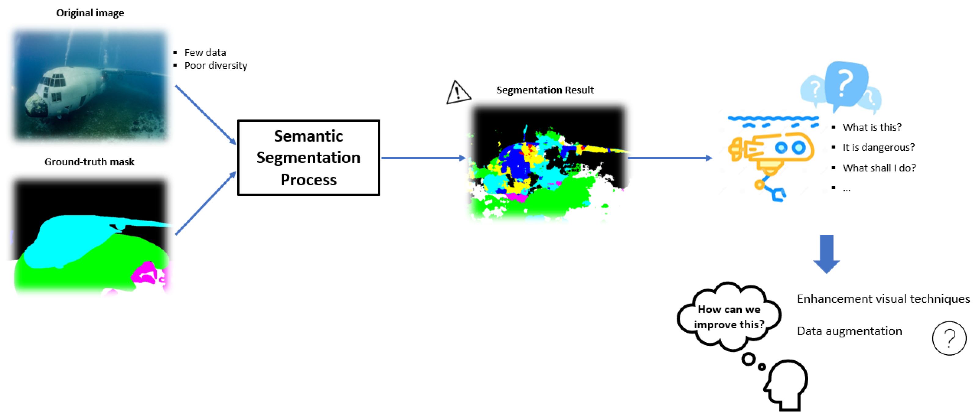
Figure 1.
Diagram of the general framework of the proposal.
Figure 1.
Diagram of the general framework of the proposal.
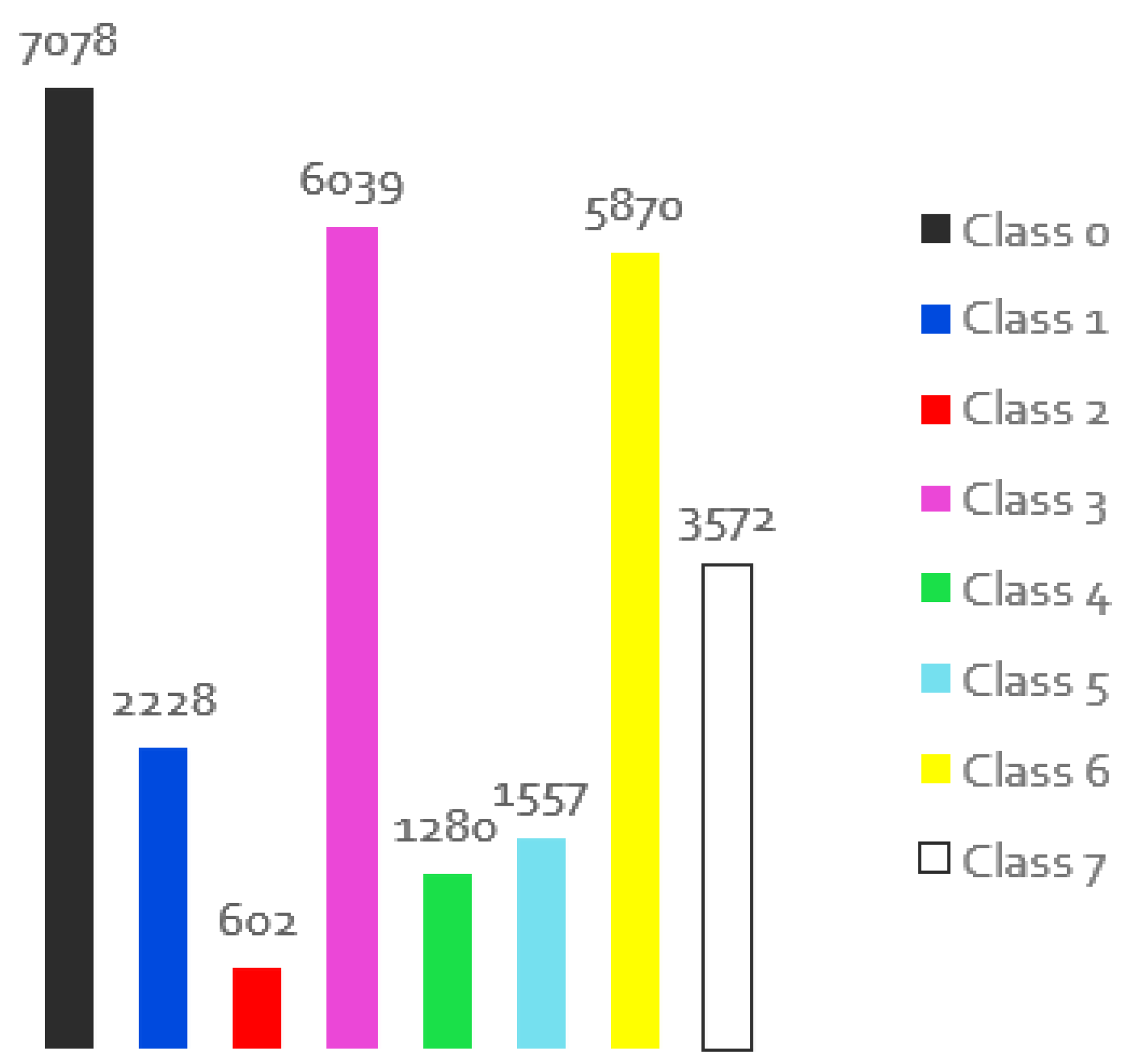
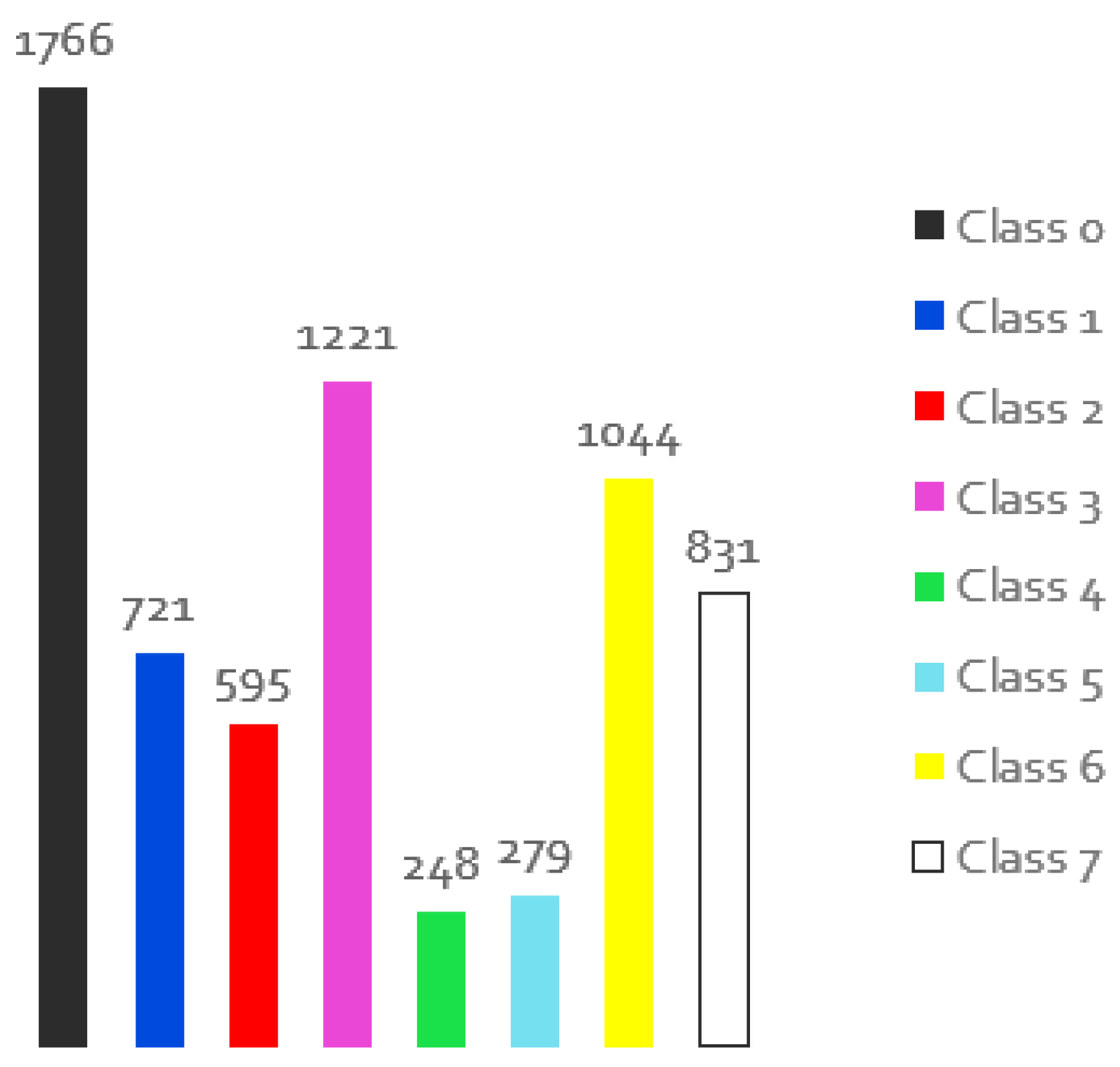
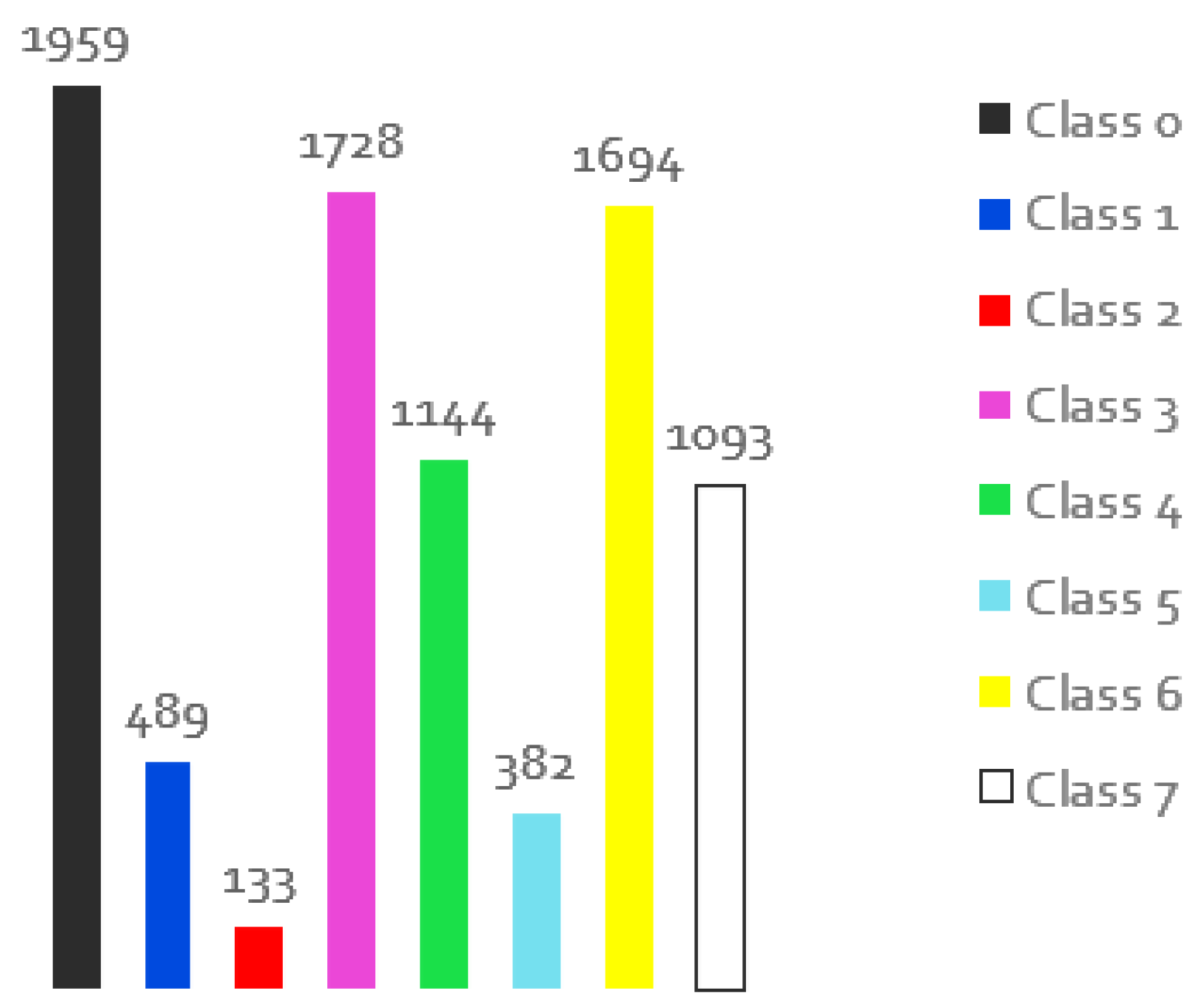
Figure 2.
Distribution of the individual classes for the images of the original training set.
Figure 2.
Distribution of the individual classes for the images of the original training set.
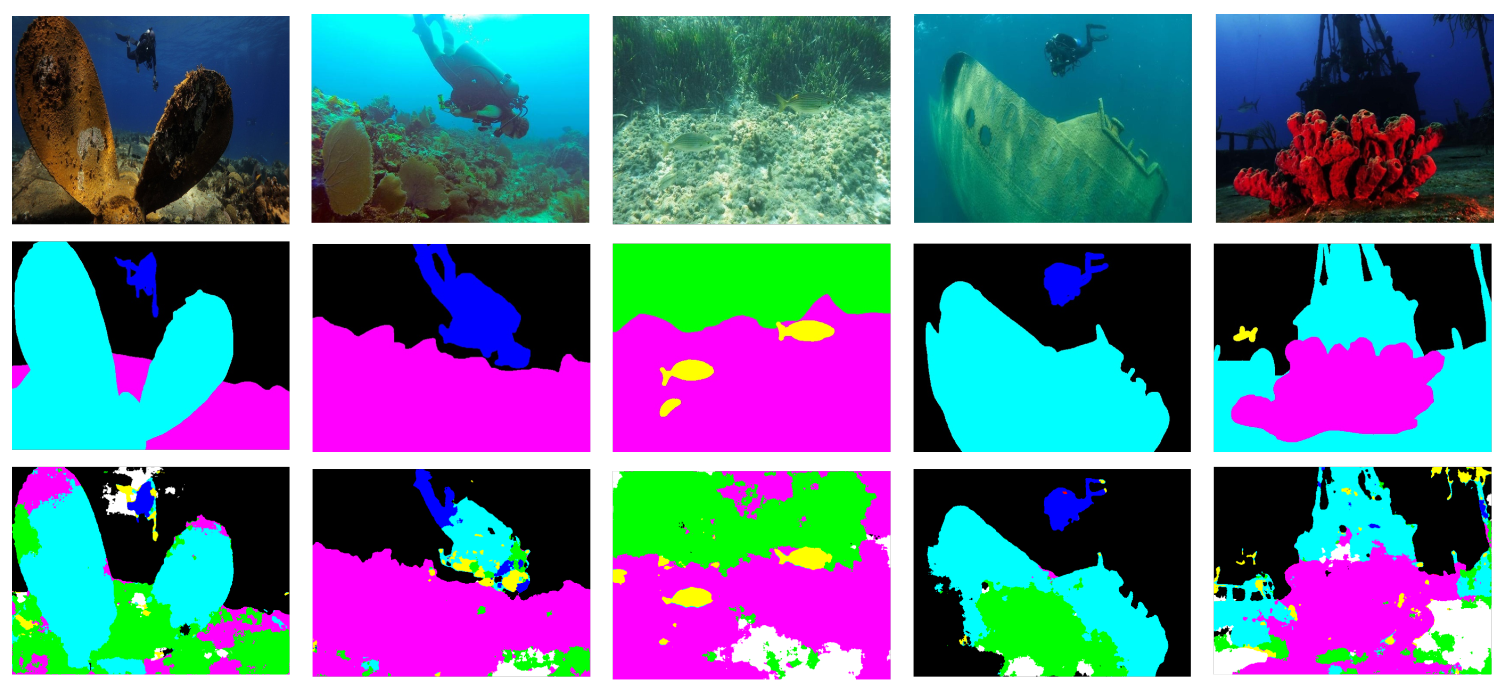
Figure 3.
The segmented images obtained with the original dataset for a total of 100 evaluations after every 500 training images are based on the best model, with each different colour representing a different class.
Figure 3.
The segmented images obtained with the original dataset for a total of 100 evaluations after every 500 training images are based on the best model, with each different colour representing a different class.
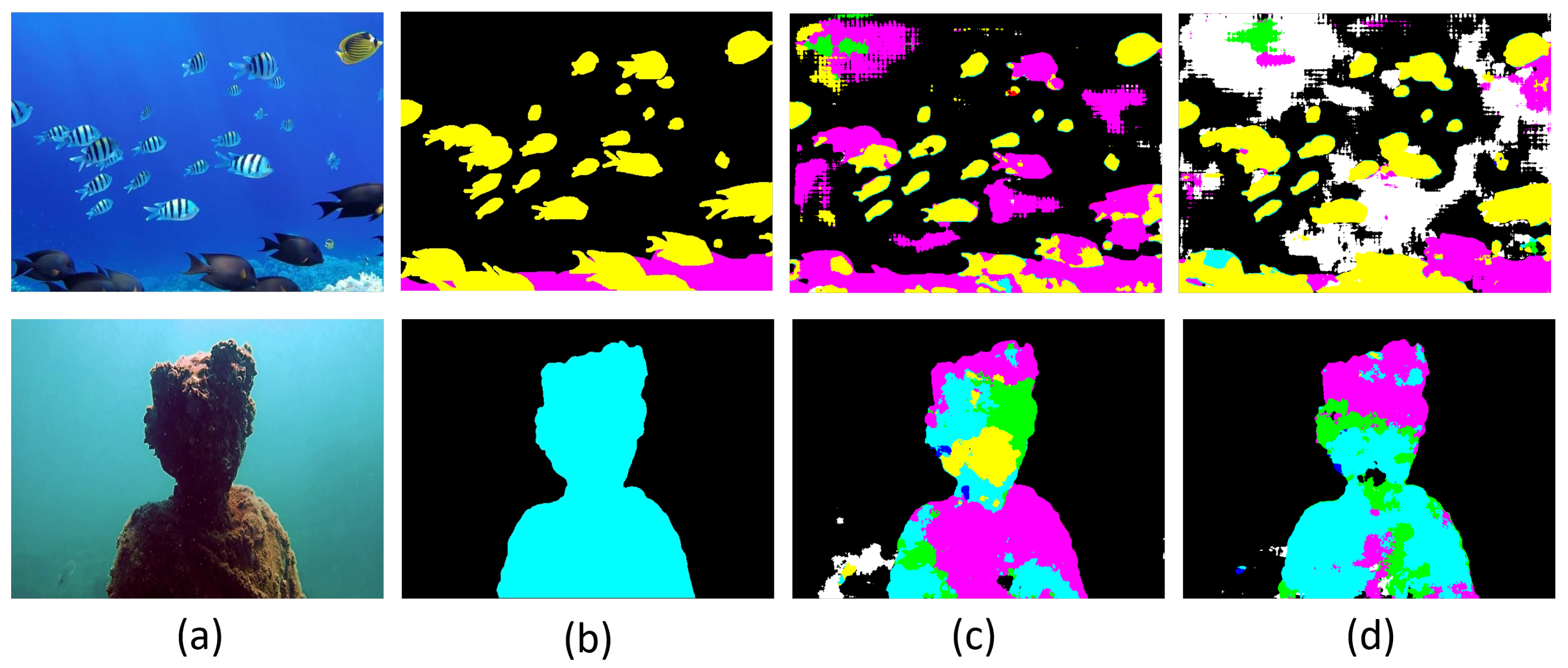
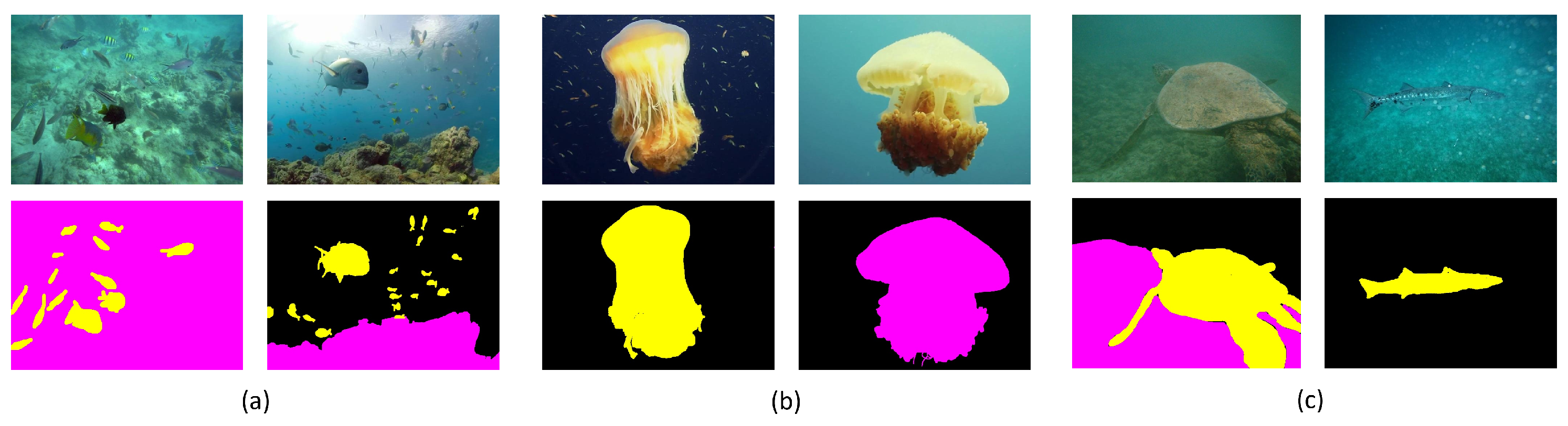
Figure 4.
Problems of the dataset: more elements of a class in the original image than in the mask (a), some labeled errors when referring to the same class (b) and poor quality of the images obtained underwater (c). The 3 colours that appear in the second row indicate the 3 classes: Fish (yellow), Reefs (pink) and Waterbody (black).
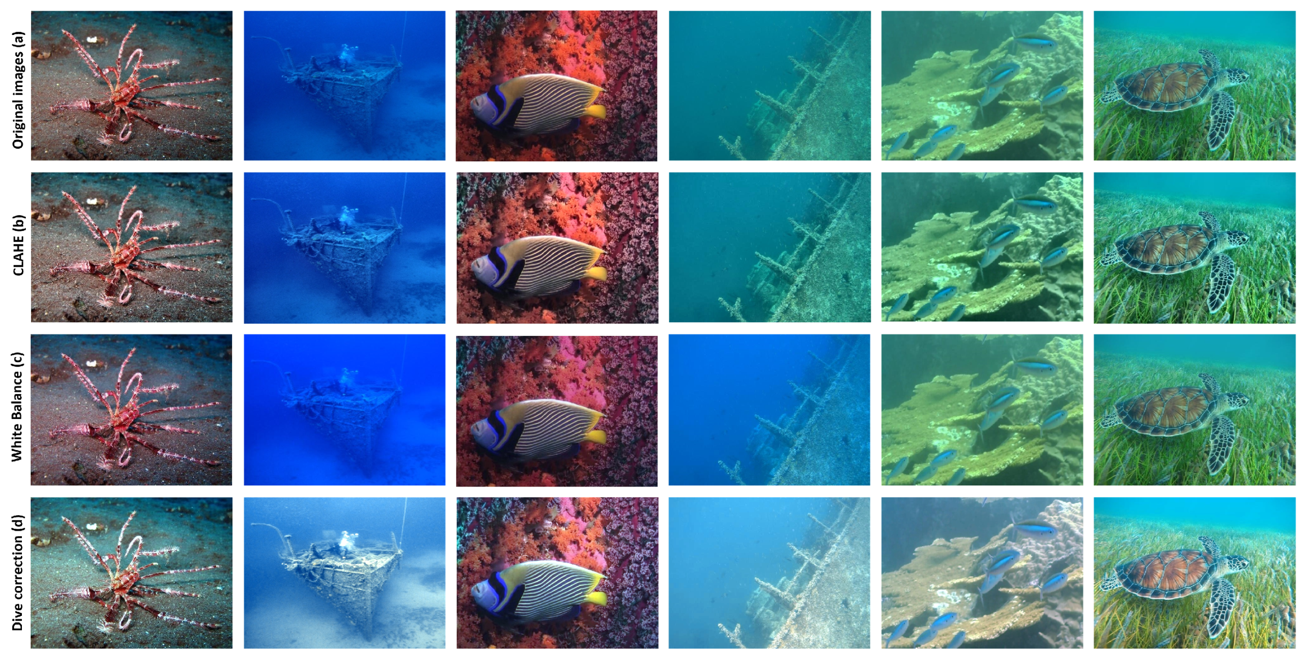
Figure 5.
Comparison of the improvement methods using 6 original images (a) with the CLAHE method (b), white balance transformation (c) and dive correction (d).
Figure 5.
Comparison of the improvement methods using 6 original images (a) with the CLAHE method (b), white balance transformation (c) and dive correction (d).
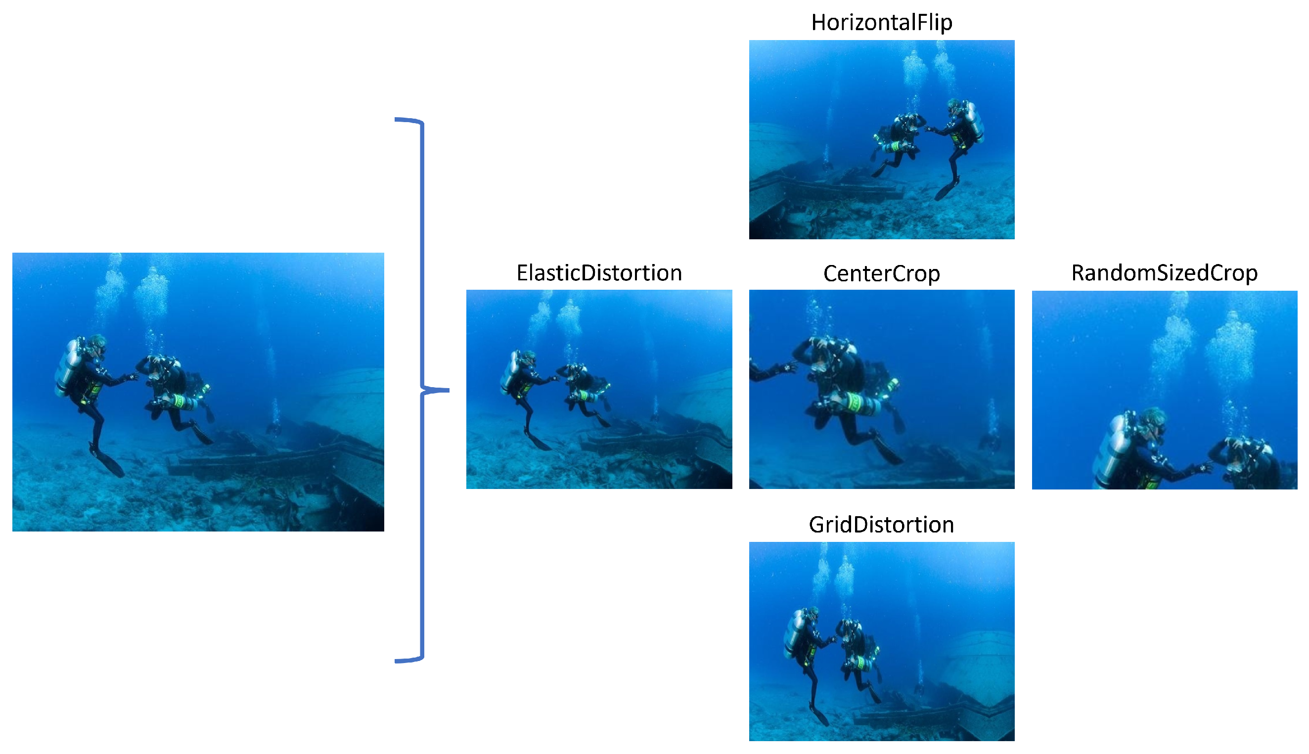
Figure 6.
Five examples of possible changes to increase the size of the dataset using a single image.
Figure 6.
Five examples of possible changes to increase the size of the dataset using a single image.
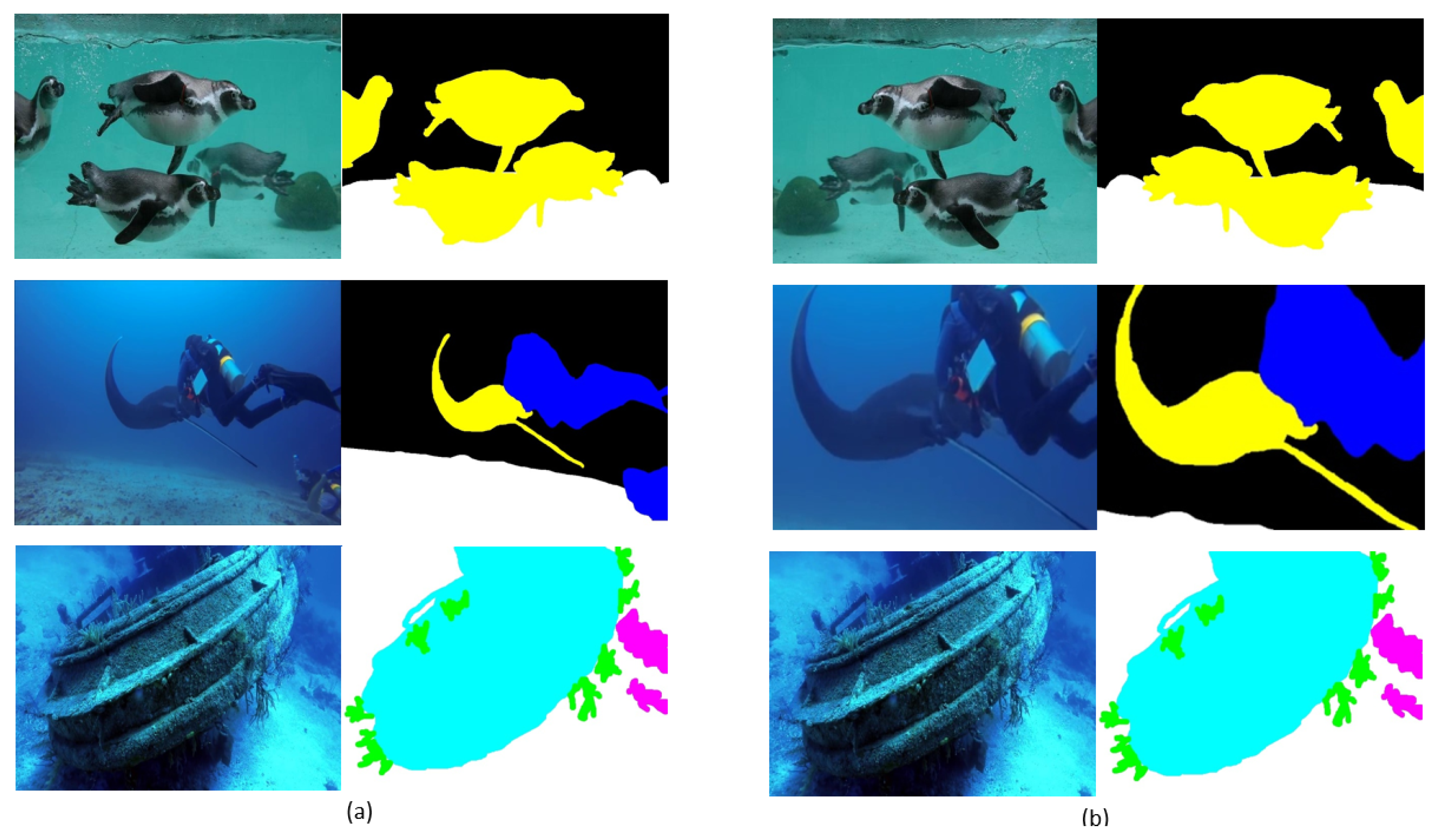
Figure 7.
Result from two original images (a): in some cases, good variations result, but at the same time images arise that do not fit into the intended context (b).
Figure 7.
Result from two original images (a): in some cases, good variations result, but at the same time images arise that do not fit into the intended context (b).
Figure 8.
Some examples of original images (a) and corresponding transformations (b) are shown. The first and second rows represent transformations by flipping and cropping, which also change the mask, and the third row represents a quality degradation where the ground truth does not need to be changed. The second columns represent the ground truth, with each colour representing a different class.
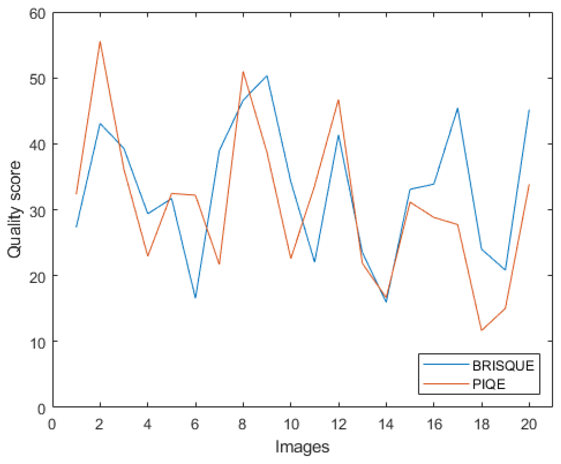
Figure 9.
Quality assessment with BRISQUE and PIQE for 20 original images selected to evaluate the quality of images processed with enhancement techniques.
Figure 9.
Quality assessment with BRISQUE and PIQE for 20 original images selected to evaluate the quality of images processed with enhancement techniques.
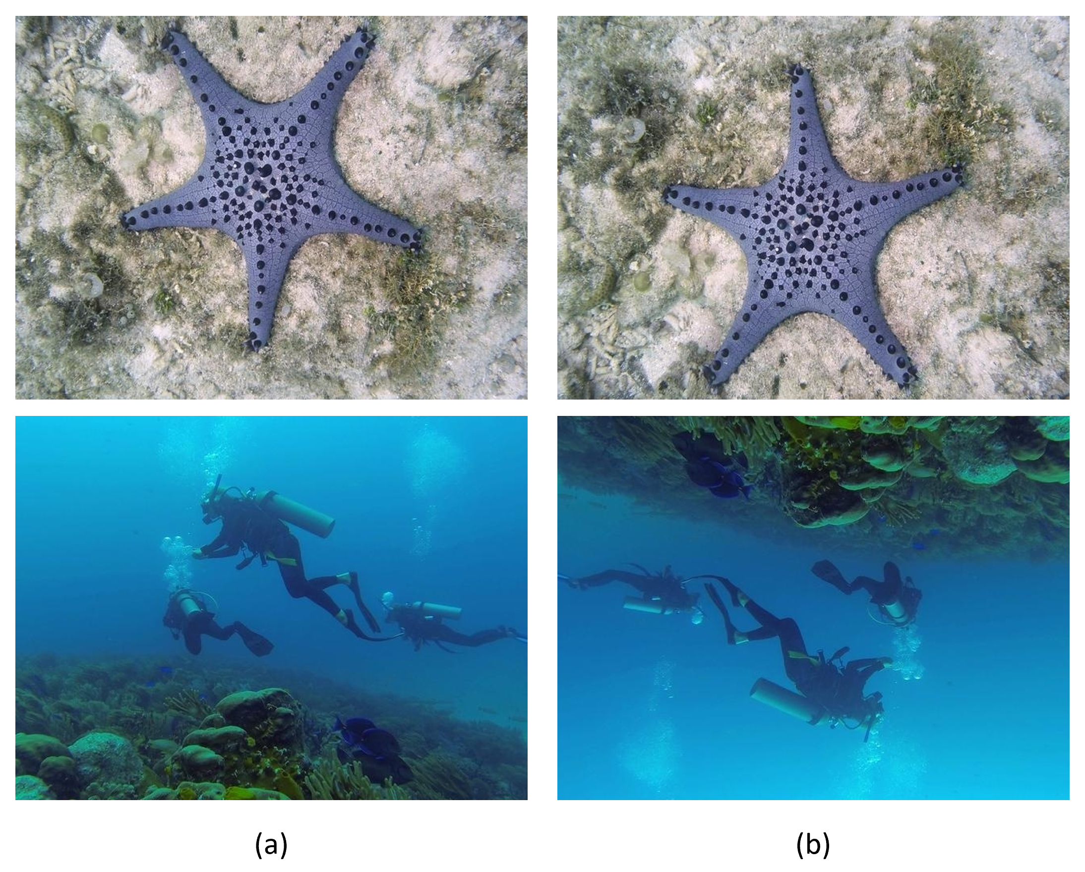
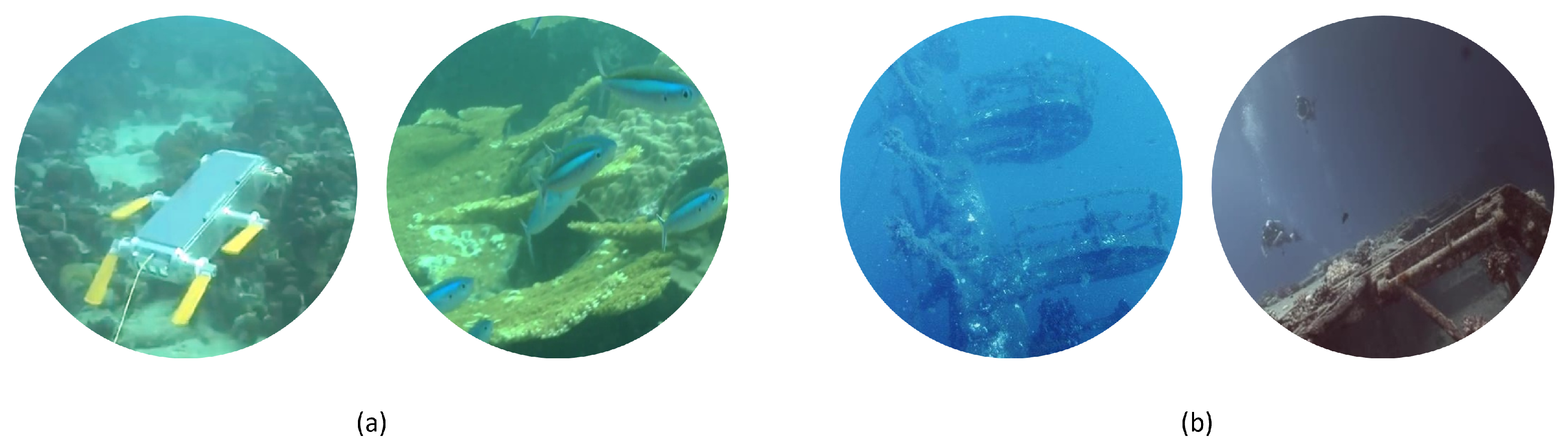
Figure 10.
Two examples of bad visual images (a) and good visual images (b) of the original set, according with the methods BRISQUE and PIQE.
Figure 10.
Two examples of bad visual images (a) and good visual images (b) of the original set, according with the methods BRISQUE and PIQE.
Figure 11.
Qualitative comparison results of 4 different examples (a,b): the CLAHE method (c), WB method (d) and dive correction (e) using the best model in a total of 100 validations, each after 500 training images. The different colours represent the different classes along the results.
Figure 11.
Qualitative comparison results of 4 different examples (a,b): the CLAHE method (c), WB method (d) and dive correction (e) using the best model in a total of 100 validations, each after 500 training images. The different colours represent the different classes along the results.
Figure 12.
Comparison of the qualitative results of 2 different examples (a,b), between the result obtained with the original set (c) and the CLAHE method (d) using the best model for a total of 100 validations. The different colours represent the different classes along the results.
Figure 12.
Comparison of the qualitative results of 2 different examples (a,b), between the result obtained with the original set (c) and the CLAHE method (d) using the best model for a total of 100 validations. The different colours represent the different classes along the results.
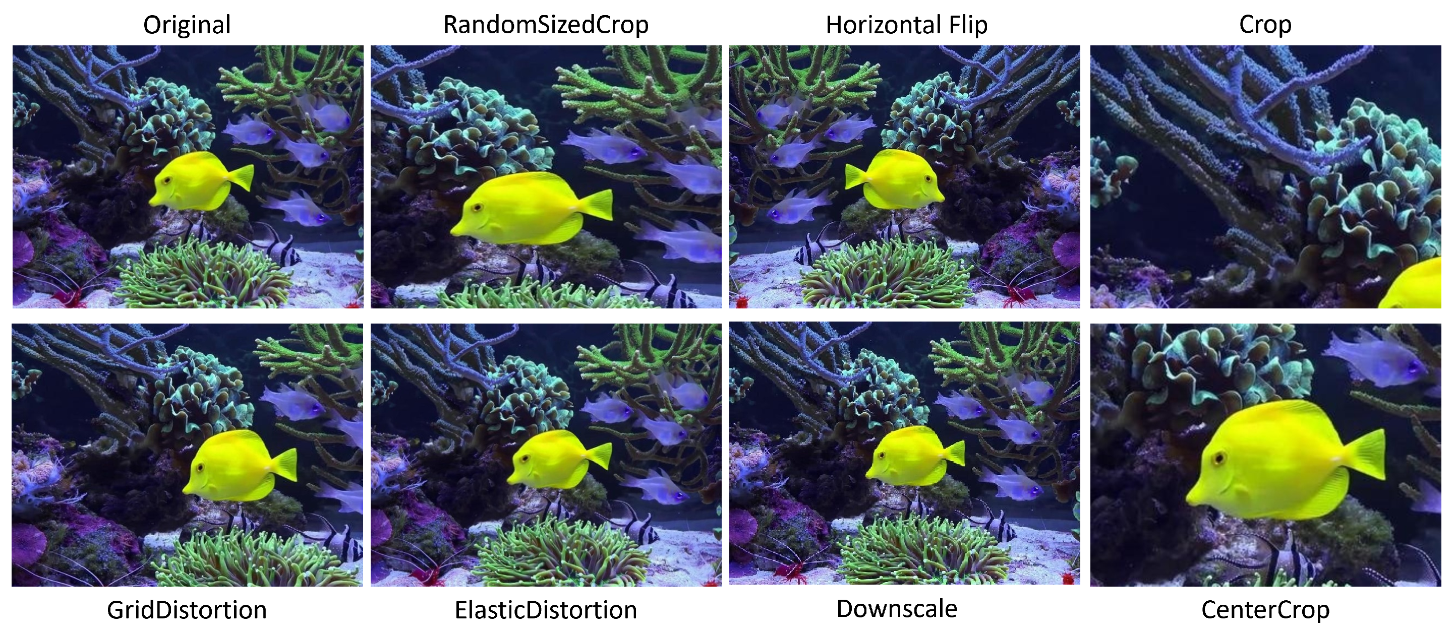
Figure 13.
Eight transformations used in the creation of the augmented datasets for training.
Figure 13.
Eight transformations used in the creation of the augmented datasets for training.
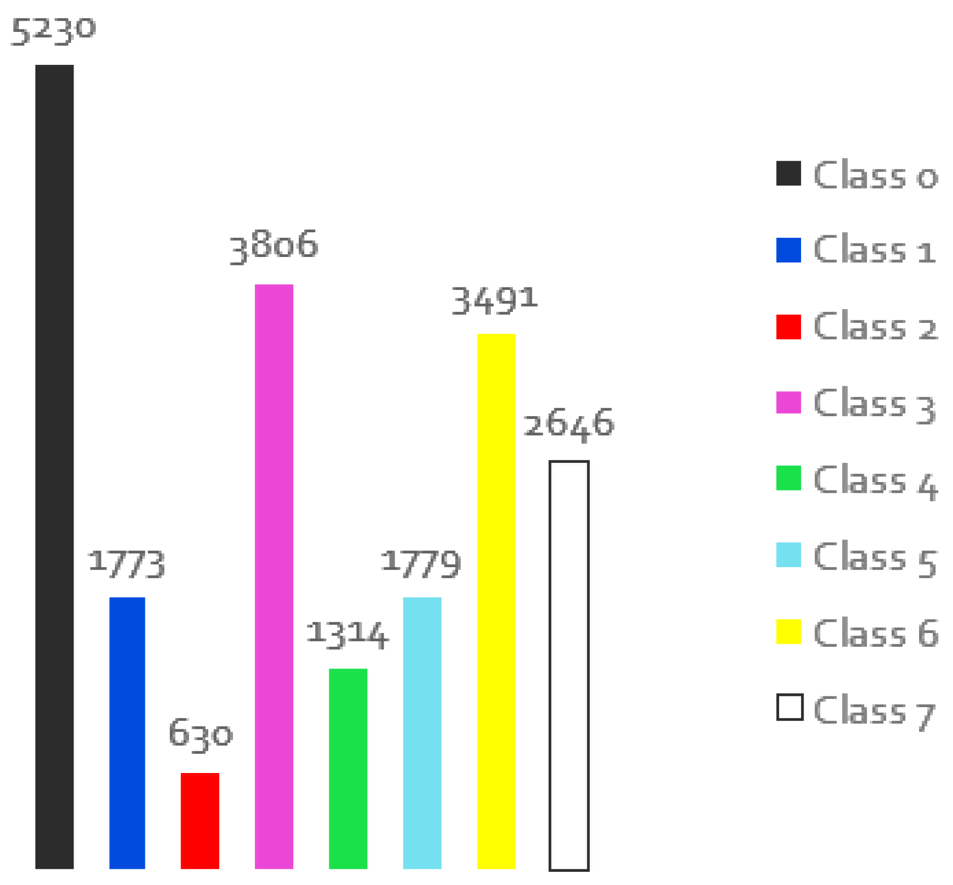
Figure 14.
Distribution of the individual classes for the images of the training set with data augmentation.
Figure 14.
Distribution of the individual classes for the images of the training set with data augmentation.
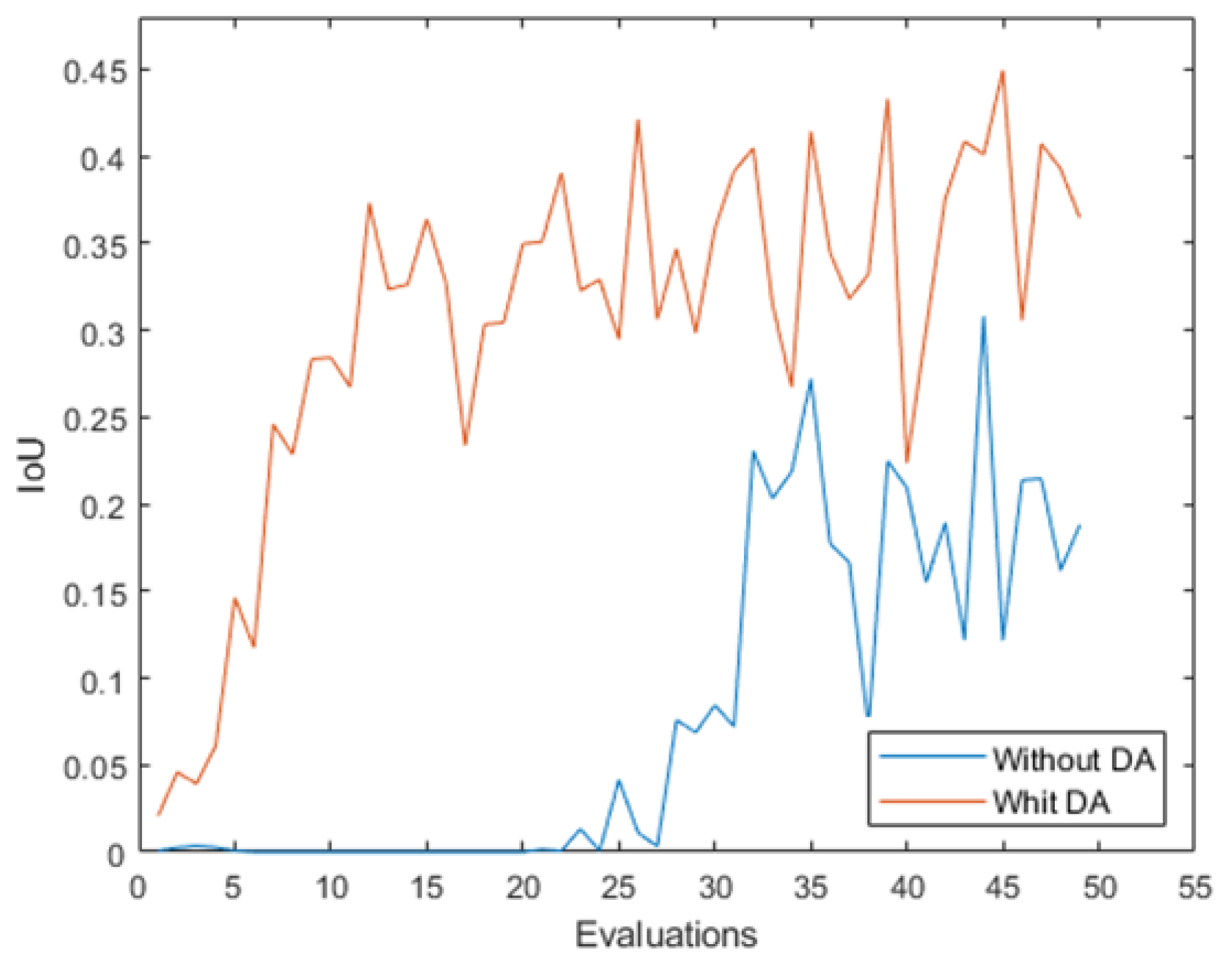
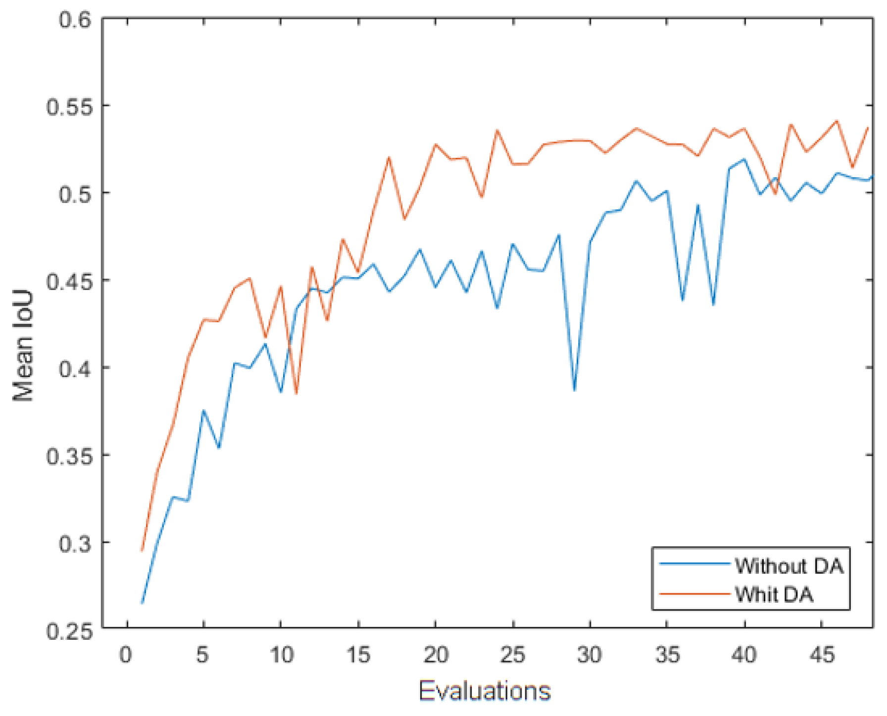
Figure 15.
Mean IoU measurement along the 50 evaluations with the original dataset and the data augmentation dataset.
Figure 15.
Mean IoU measurement along the 50 evaluations with the original dataset and the data augmentation dataset.
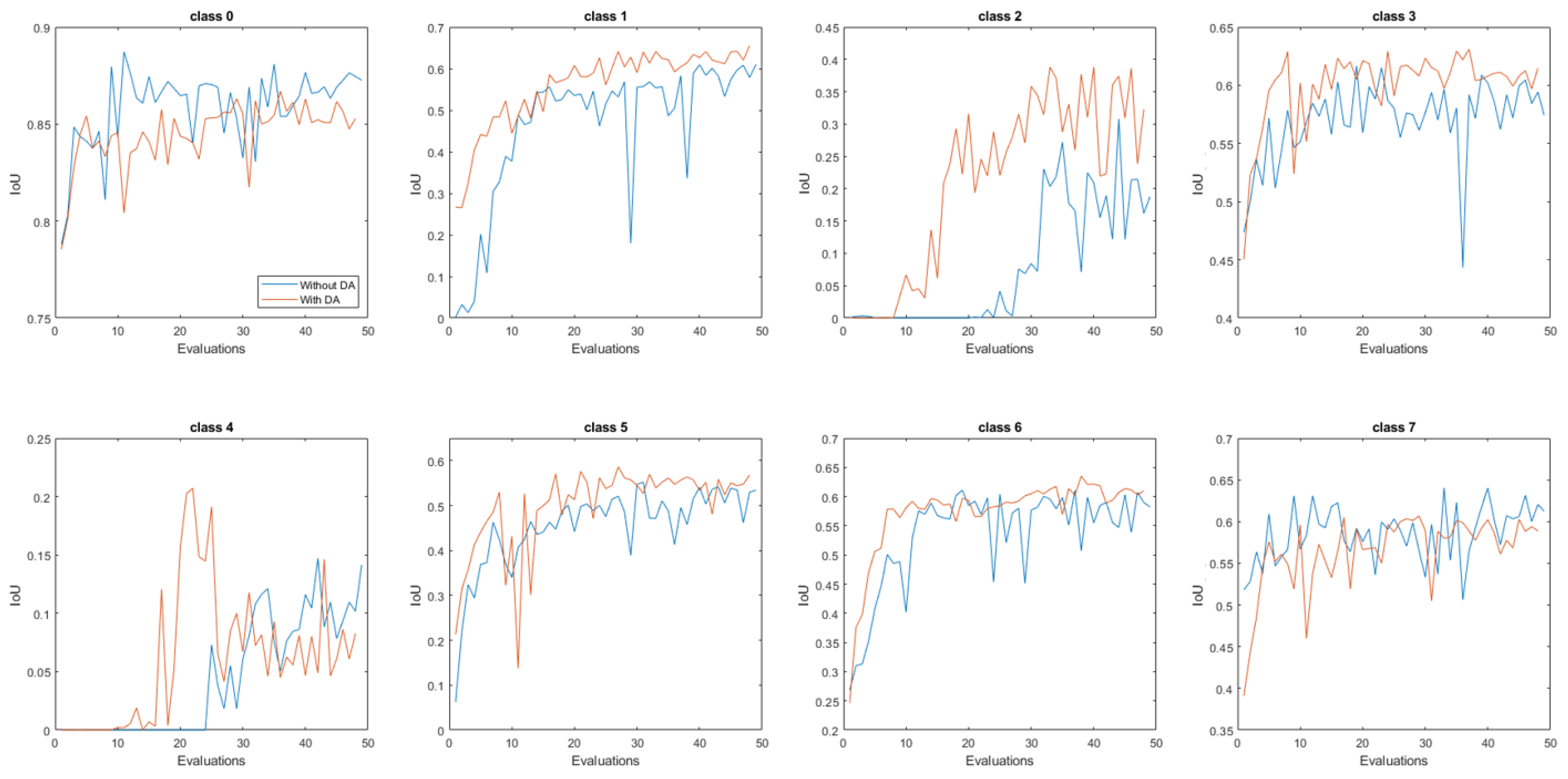
Figure 16.
IoU measurement along the 50 evaluations with the original dataset and the data augmentation dataset, for each class.
Figure 16.
IoU measurement along the 50 evaluations with the original dataset and the data augmentation dataset, for each class.
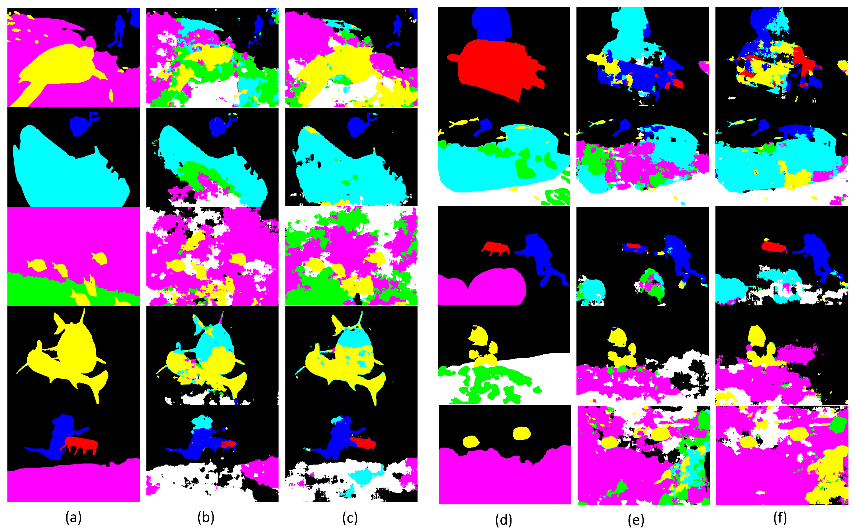
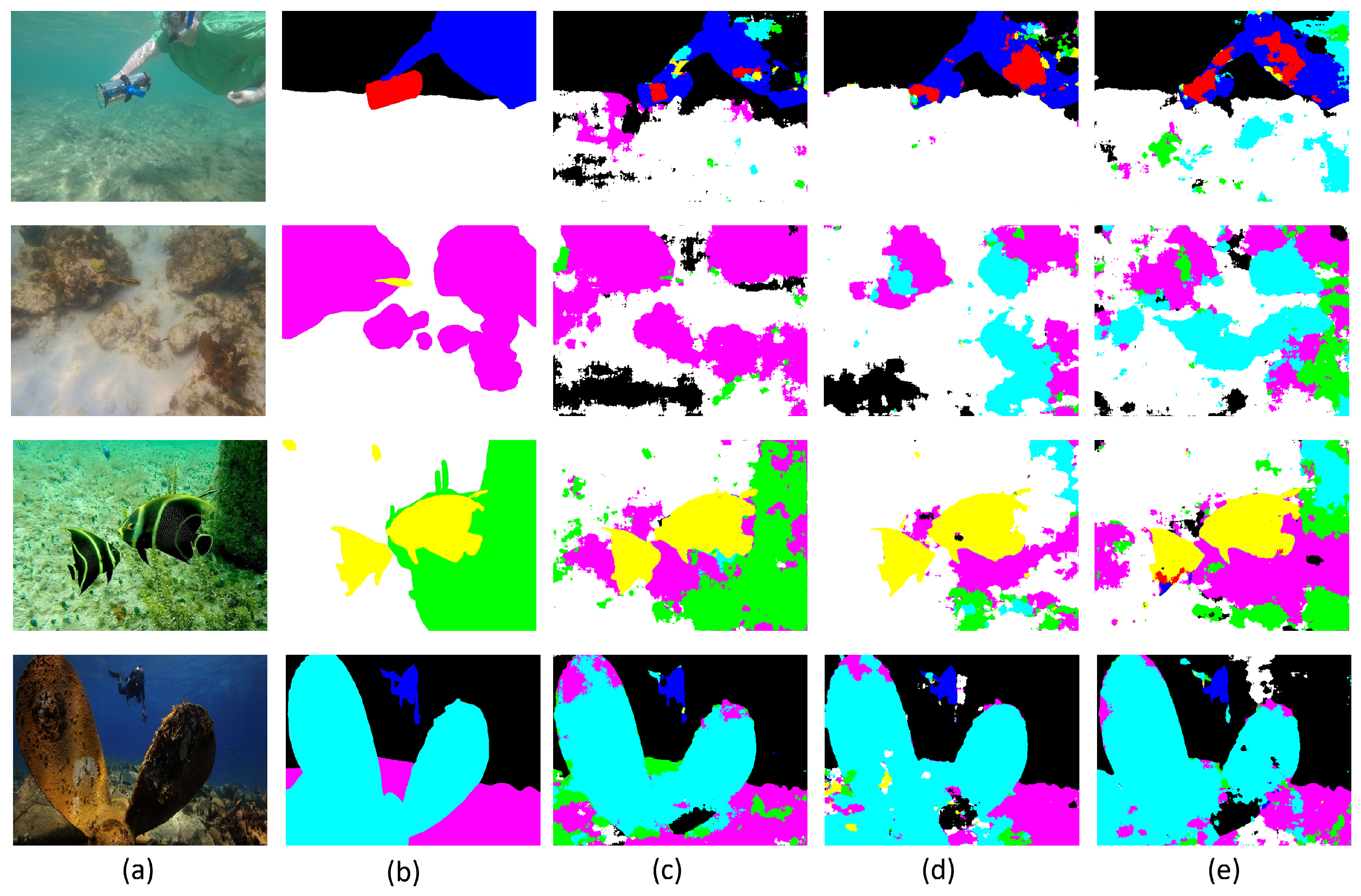
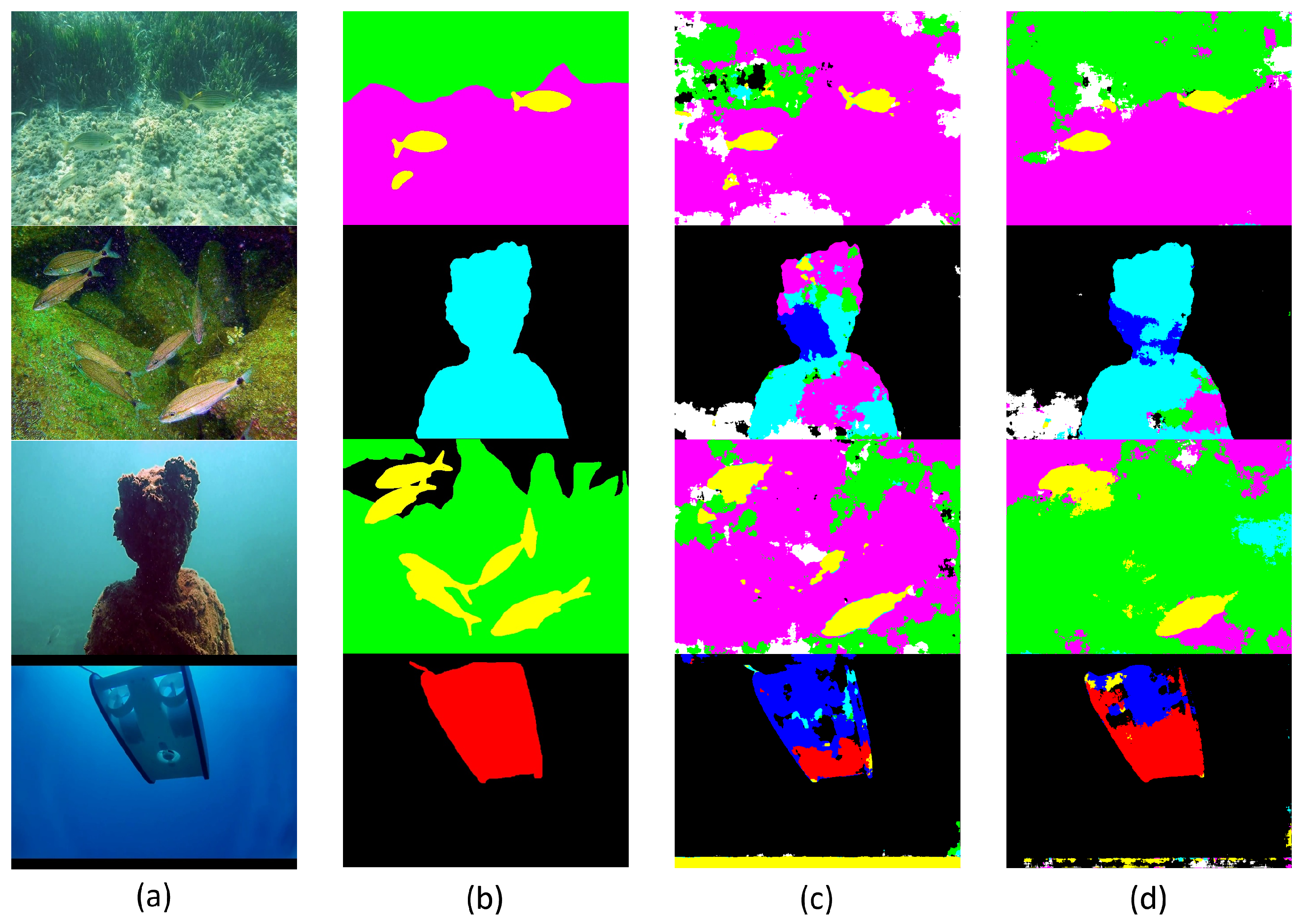
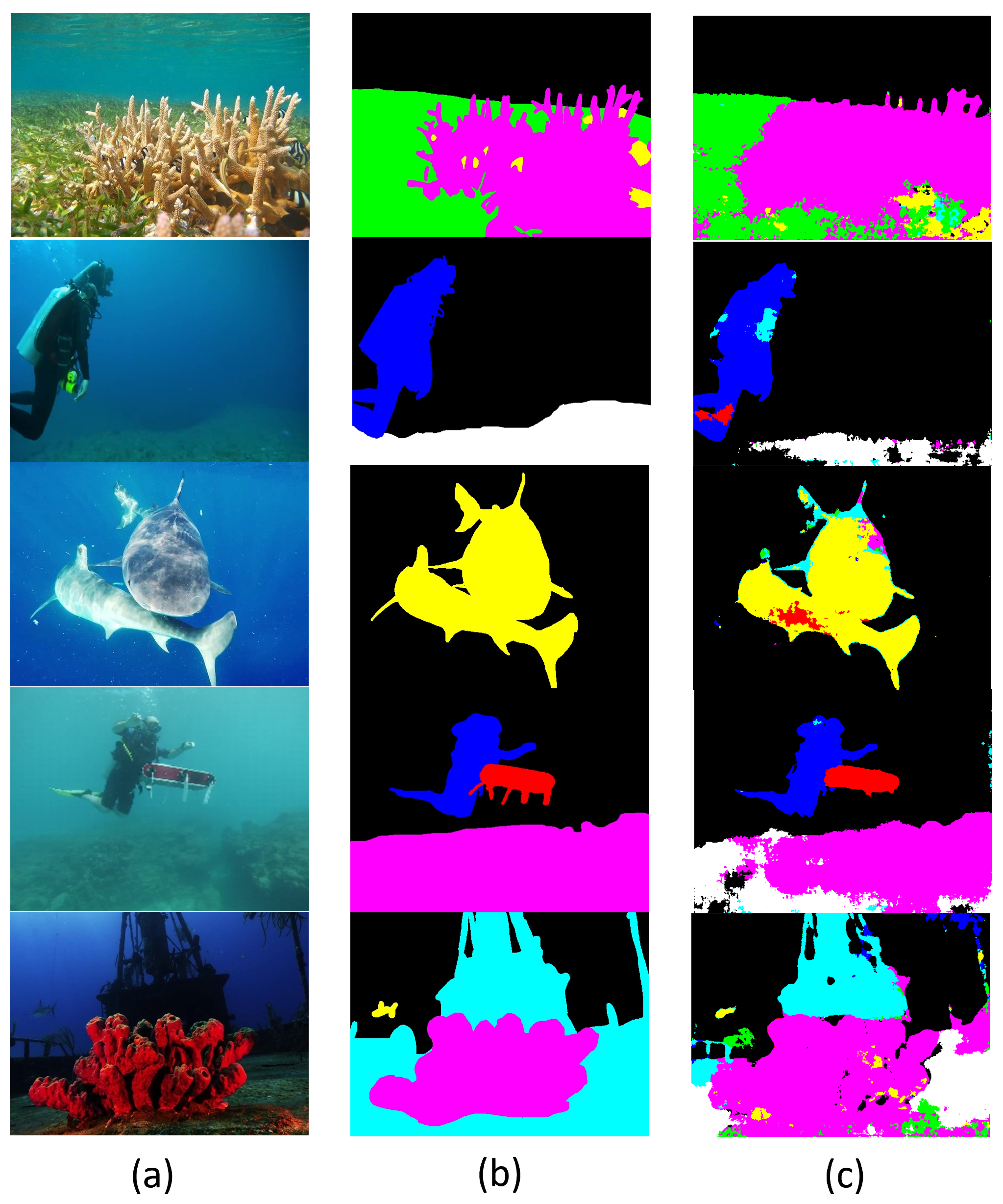
Figure 17.
Qualitative comparison of the results of 10 different examples of semantic segmentation (a,d) using the original dataset (b,e) and the data augmentation set (c,f) for the training process, in which the best model was selected in a total of 50 validations. The different colours represent the different predicted classes along the results.
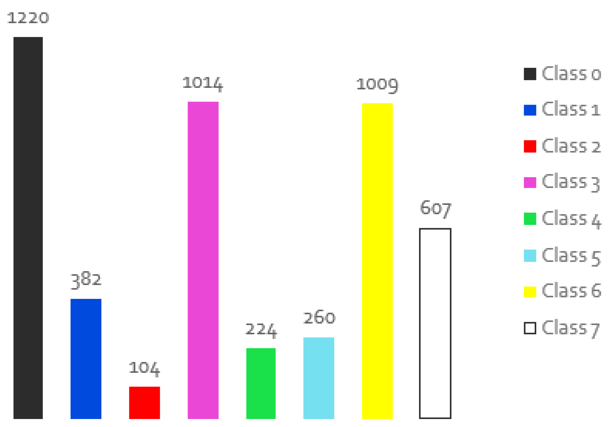
Figure 18.
Distribution of the individual classes for the images of the training set when applying the data augmentation in different numbers according to the class.
Figure 18.
Distribution of the individual classes for the images of the training set when applying the data augmentation in different numbers according to the class.
Figure 19.
Qualitative comparison results of 4 different examples of semantic segmentation (a,b), obtained from the original training set (c) and the data augmentation set (d), using the best model in a total of 50 validations for each case. The different colours represent the different predicted classes along the results.
Figure 20.
Distribution of the individual classes for the images of the training set when applying the data augmentation only in the robot class.
Figure 20.
Distribution of the individual classes for the images of the training set when applying the data augmentation only in the robot class.
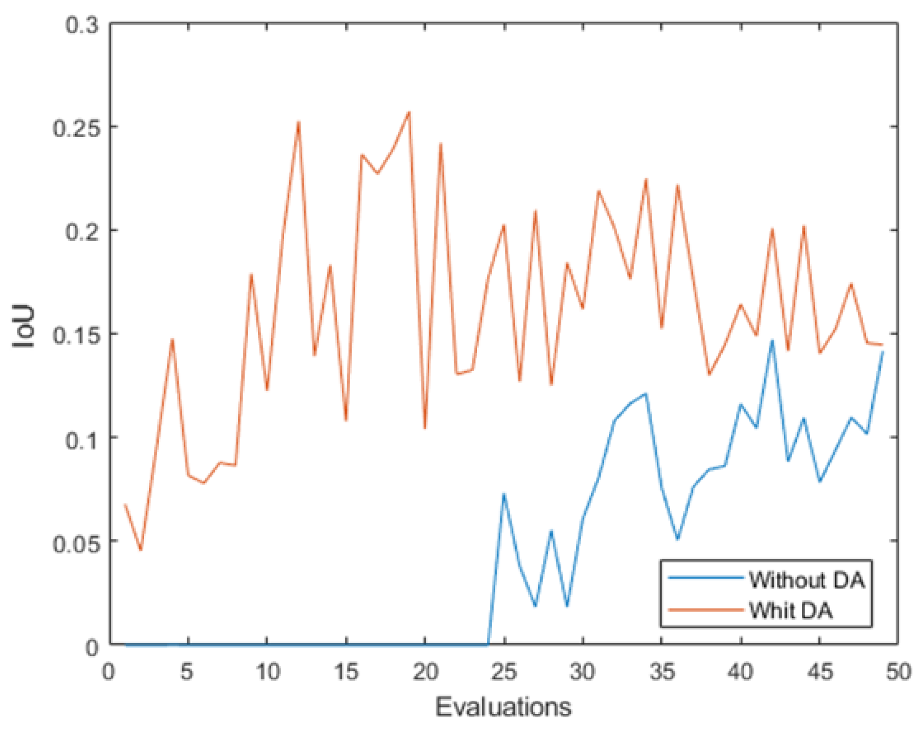
Figure 21.
IoU measurement for the robot class (class 2) along the 50 evaluations with the original dataset and the data augmentation dataset.
Figure 21.
IoU measurement for the robot class (class 2) along the 50 evaluations with the original dataset and the data augmentation dataset.
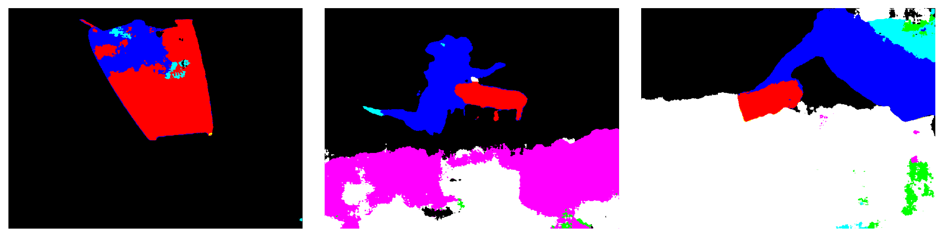
Figure 22.
Qualitative results of different examples of segmented image with robots, obtained from the data augmentation set for the robot class, using the best model in a total of 50 validations. The different colours represent the different predicted classes along the results.
Figure 22.
Qualitative results of different examples of segmented image with robots, obtained from the data augmentation set for the robot class, using the best model in a total of 50 validations. The different colours represent the different predicted classes along the results.
Figure 23.
Demonstration of the size and location on the original set of the plants in some of the images. The different colours represent the different classes in the original masks.
Figure 23.
Demonstration of the size and location on the original set of the plants in some of the images. The different colours represent the different classes in the original masks.
Figure 24.
Distribution of the individual classes for the images of the training set when applying the data augmentation only in the plant class.
Figure 24.
Distribution of the individual classes for the images of the training set when applying the data augmentation only in the plant class.
Figure 25.
IoU measurement for the plant class (class 4) along the 50 evaluations with the original dataset and the data augmentation dataset.
Figure 25.
IoU measurement for the plant class (class 4) along the 50 evaluations with the original dataset and the data augmentation dataset.
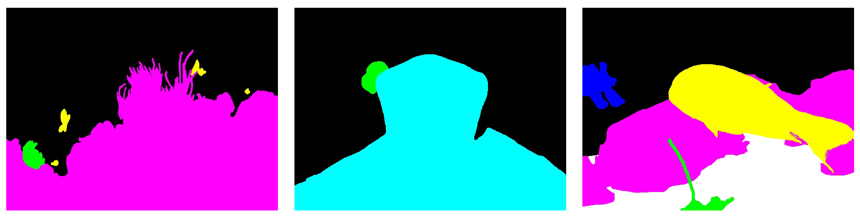
Figure 26.
Results of 5 different examples of semantic segmentation (a,b), obtained from the use of both strategies at the same time: data augmentation of the less representative classes and CLAHE method (c). The different colours represent the different classes in the original masks and predicted results.
Table 1.
Performance measurements [%] for the best result obtained with the original dataset in a total of 100 evaluations.
Table 1.
Performance measurements [%] for the best result obtained with the original dataset in a total of 100 evaluations.
| Overall Acc | Mean Acc | Mean IoU | IoU 0 | IoU 1 | IoU 2 | IoU 3 | IoU 4 | IoU 5 | IoU 6 | IoU 7 |
|---|
| 79.7 | 64.4 | 53.1 | 87.2 | 62.7 | 29.5 | 58.8 | 16.6 | 51.6 | 59.1 | 69.6 |
Table 2.
Comparative results of the mean of the quality score of the Dive, WB and CLAHE corrections for a total of 20 images, using PIQE, BRISQUE, NIQE and the sr_metric. For each metric, the results that exceed the results obtained with the original set are highlighted in bold.
Table 2.
Comparative results of the mean of the quality score of the Dive, WB and CLAHE corrections for a total of 20 images, using PIQE, BRISQUE, NIQE and the sr_metric. For each metric, the results that exceed the results obtained with the original set are highlighted in bold.
| Data | PIQE | BRISQUE | NIQE | sr_metric |
|---|
| Original | 30.63 | 33.14 | 3.30 | 6.35 |
| Dive | 31.9 | 30.16 | 3.15 | 7.27 |
| WB | 36.7 | 37.45 | 3.38 | 5.92 |
| CLAHE | 32.50 | 27.50 | 3.14 | 7.40 |
Table 3.
Comparative results of best measured model performance [%] achieved with CLAHE, WB and dive corrections in a total of 100 validations, each after 500 training images. Whenever the results achieved exceed the results of the original set, they are emphasised in bold.
Table 3.
Comparative results of best measured model performance [%] achieved with CLAHE, WB and dive corrections in a total of 100 validations, each after 500 training images. Whenever the results achieved exceed the results of the original set, they are emphasised in bold.
| Method | Overall Acc | Mean Acc | Mean IoU | IoU 0 | IoU 1 | IoU 2 | IoU 3 | IoU 4 | IoU 5 | IoU 6 | IoU 7 |
|---|
| Original | 79.7 | 64.4 | 53.1 | 87.2 | 62.7 | 29.5 | 58.8 | 16.6 | 51.6 | 59.1 | 69.6 |
| CLAHE | 80.4 | 64.0 | 53.3 | 87.0 | 61.6 | 25.7 | 59.1 | 14.1 | 54.2 | 60.5 | 64.2 |
| WB | 80.0 | 62.5 | 51.9 | 86.6 | 58.2 | 30.0 | 59.7 | 8.5 | 55.8 | 56.8 | 59.4 |
| Dive | 80.5 | 63.4 | 52.3 | 87.1 | 58.2 | 27.4 | 60.0 | 11.6 | 53.9 | 57.6 | 62.8 |
Table 4.
Performance measures [%] for the best result obtained with the original dataset and the dataset with data augmentation in a total of 50 validations. In bold type, you can see for each class whether the results achieved with the data augmentation are better than the original results.
Table 4.
Performance measures [%] for the best result obtained with the original dataset and the dataset with data augmentation in a total of 50 validations. In bold type, you can see for each class whether the results achieved with the data augmentation are better than the original results.
| | Overall Acc | Mean Acc | Mean IoU | IoU 0 | IoU 1 | IoU 2 | IoU 3 | IoU 4 | IoU 5 | IoU 6 | IoU 7 |
|---|
| Original | 80.6 | 62.9 | 51.8 | 87.6 | 60.9 | 20.9 | 60.2 | 11.6 | 54.1 | 55.5 | 64.0 |
| DA | 80.4 | 65.0 | 54.1 | 85.7 | 64.2 | 38.6 | 61.3 | 8.6 | 54.3 | 61.1 | 58.8 |
Table 5.
Performance measures [%] for the best result obtained with the original dataset and the new dataset with data augmentation (DA1) in a total of 50 validations. In bold type, you can see for each class whether the results achieved with the data augmentation are better than the original results.
| | Overall Acc | Mean Acc | Mean IoU | IoU 0 | IoU 1 | IoU 2 | IoU 3 | IoU 4 | IoU 5 | IoU 6 | IoU 7 |
|---|
| Original | 80.6 | 62.9 | 51.8 | 87.6 | 60.9 | 20.9 | 60.2 | 11.6 | 54.1 | 55.5 | 64.0 |
| DA1 | 80.2 | 66.0 | 54.4 | 86.3 | 61.1 | 37.7 | 61.2 | 23.5 | 53.4 | 54.8 | 57.9 |
Table 6.
Performance metrics [%] comparison for the best result with the more balanced dataset with data augmentation (DA) and this dataset with CLAHE method (DA_C) applied for a total of 50 validations. For each result, you can see whether using both strategies is better (in bold) than using only the data augmentation.
| | Overall Acc | Mean Acc | Mean IoU | IoU 0 | IoU 1 | IoU 2 | IoU 3 | IoU 4 | IoU 5 | IoU 6 | IoU 7 |
|---|
| DA1 | 80.2 | 66.0 | 54.4 | 86.3 | 61.1 | 37.7 | 61.2 | 23.5 | 53.4 | 54.8 | 57.9 |
| DA_C | 81.8 | 67.6 | 56.0 | 87.9 | 66.7 | 39.4 | 62.4 | 12.8 | 53.9 | 61.0 | 63.9 |


