Deep Learning Applications in Vessel Dead Reckoning to Deal with Missing Automatic Identification System Data

Abstract

This research introduces an online system for monitoring maritime traffic, aimed at tracking vessels in water routes and predicting their subsequent locations in real time. The proposed framework utilizes an Extract, Transform, and Load (ETL) pipeline to dynamically process AIS data by cleaning, compressing, and enhancing it with additional attributes such as online traffic volume, origin/destination, vessel trips, trip direction, and vessel routing. This processed data, enriched with valuable details, serves as an alternative to raw AIS data stored in a centralized database. For user interactions, a user interface is designed to query the database and provide real-time information on a map-based interface. To deal with false or missing AIS records, two methods, dead reckoning and machine learning techniques, are employed to anticipate the trajectory of the vessel in the next time steps. To evaluate each method, several metrics are used, including R squared, mean absolute error, mean offset, and mean offset from the centerline. The functionality of the proposed system is showcased through a case study conducted in the Gulf Intracoastal Waterway (GIWW). Three years of AIS data are collected and processed as a simulated API to transmit AIS records every five minutes. According to our results, the Seq2Seq model exhibits strong performance (0.99 R squared and an average offset of ~1400 ft). However, the second scenario, dead reckoning, proves comparable to the Seq2Seq model as it involves recalculating vessel headings by comparing each data point with the previous one.

1. Introduction

The availability of maritime data, collected through an extensive network of terrestrial and satellite Automatic Identification System (AIS) receivers, has created unprecedented opportunities for transformative analyses and the extraction of valuable insights in maritime traffic monitoring. This abundance of information enables various crucial applications, including vessel trajectory prediction, anomaly detection, threat assessment, and tracking and classification of maritime activities [1].

At the core of this data-driven revolution is AIS technology, which plays a central role in maritime operations for real-time tracking and monitoring of vessels. Utilizing Very High Frequency (VHF) signals, AIS facilitates the exchange of encoded information containing various attributes of a ship at regular intervals. These attributes include key details such as the ship’s position coordinates, speed over ground, course over ground, Maritime Mobile Service Identities (MMSI), and more. AIS data are categorized into static and dynamic information, with static details encompassing essential ship-related information and dynamic data continuously transmitted and varying based on the vessel’s motion [2,3].

The management challenges posed by the high volume and velocity of AIS data underscore the necessity for compression and efficient data processing. The frequent transmission of AIS signals generates substantial data, posing challenges for real-time analysis, decision-making procedures, and the development of intelligent services and applications [4]. To tackle this issue, compression techniques are applied to reduce storage and computing costs associated with processing AIS data. These techniques aim to decrease the overall data volume by retaining essential information while eliminating redundant or negligible data points [5].

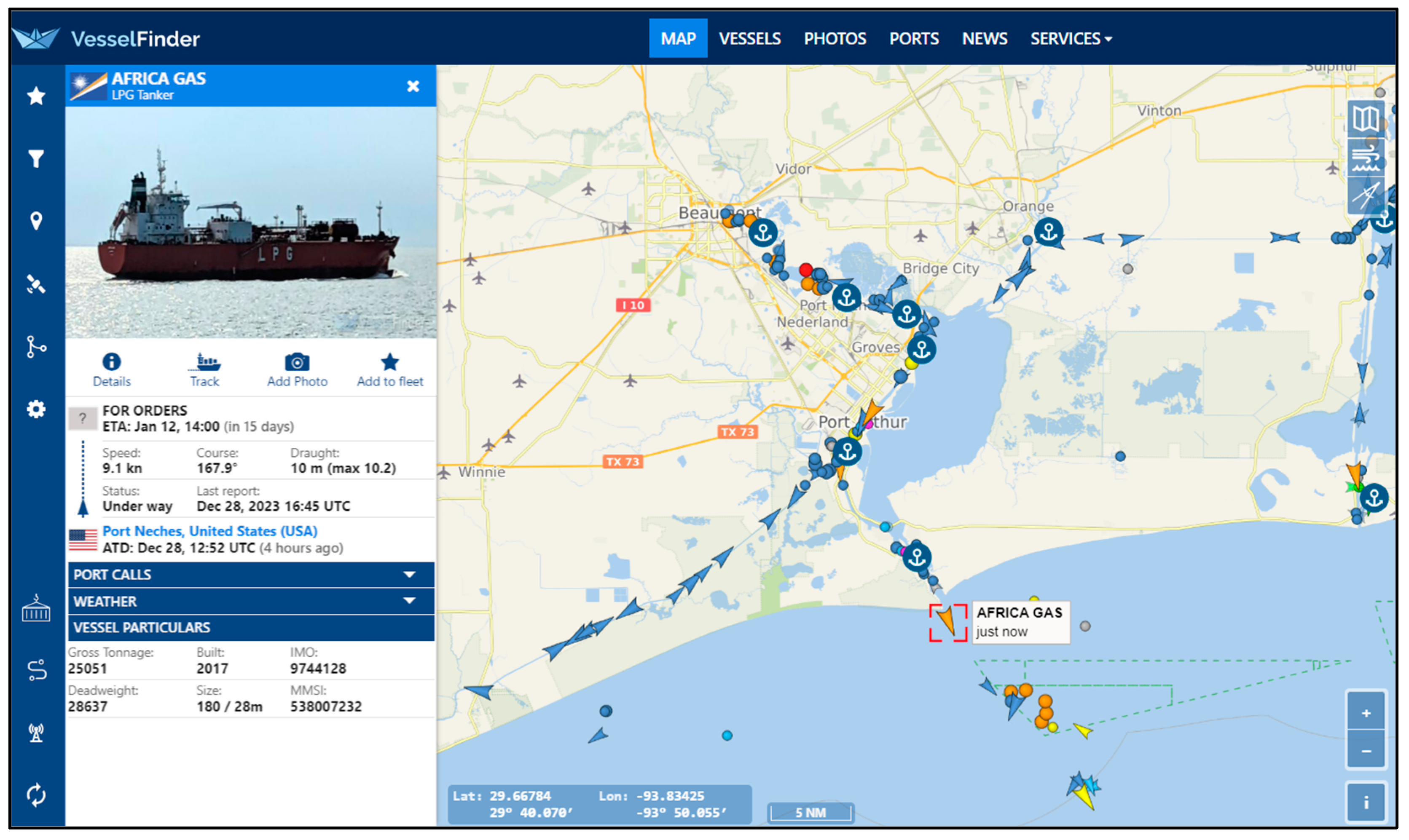
In the practical landscape of vessel monitoring, existing systems such as VesselFinder [6], Marine Cadastre [7], and AccessAIS [8], as outlined in

Table 1. Comparison of current marine systems and our proposed system.

		Features
		Real-Time Map	Historical Analysis	Real-Time Analysis	Traffic Analysis	Data Volume Reduction	Dealing with Missing Records
Current systems	VesselFinder	✓
	Marine Cadastre	✓
	AccessAIS	✓
Proposed system	ETL pipeline	✓	✓	✓	✓	✓	✓

, demonstrate capabilities in vessel tracking. In Figure 1, the dashboard of the VesselFinder platform is shown. Such systems let users find vessel locations and some static information like a vessel’s name, picture (if any), speed, destination (if provided), as well as estimated time of arrival (ETA). However, the current systems exhibit deficiencies in real-time analysis, data compression, and traffic analysis. To address these limitations, a novel system has been crafted. The proposed system not only monitors vessel movements but also conducts real-time data analysis, presenting the results on an interactive map. Additionally, the system is equipped to analyze historical data, enhancing its overall functionality.

In narrow waterways and channels, where operational intricacies are heightened, the significance of missing AIS points becomes even more pronounced. The scheduling of vessels in such areas often relies heavily on manual intervention and observation, lacking a systematic monitoring approach. Aside from manual scheduling, current Collision Avoidance Systems rely on observers to ensure safe navigation. The 1972 Convention (COLREGs) was a significant effort, introducing rules and guidelines governing vessel conduct, lights, sounds, and exemptions. The integration of advanced technologies like radar, AIS, and automatic radar plotting aid (ARPA) could provide maritime operators with real-time data, predictive tools, and automated alerts. However, these systems heavily depend on the accuracy and consistency of data inputs. AIS provides the major source of data, and any technical issues, data errors, or data absence can weaken the system’s effectiveness. Apart from vessels that are not required to have an AIS transporter, there is a notable occurrence of AIS transponders intentionally or accidentally turning off. This adds a layer of complexity, as the absence of real-time vessel information can pose significant challenges for ensuring safe navigation. Our study introduces an intelligent framework designed to track vessel traffic effectively and predict the next location of vessel movements accurately in real time. The algorithm employs an Extract, Transform, and Load (ETL) pipeline to dynamically clean, compress, and process AIS data. Furthermore, it enriches raw AIS data with valuable information such as online traffic volume, origin/destination details, vessel trips, trip directions, and vessel routing. By storing the processed data in a database, this advanced system could be a replacement for the current of collecting and storing raw AIS data. To facilitate user interactions and access to the system’s intelligent services, we have developed a user interface that allows end users to query the database and retrieve real-time information displayed on an interactive map. This intuitive interface empowers users to make informed decisions and gain valuable insights.

In the second phase of our study, we use processed data to predict the next location of vessel movements employing two distinct approaches: classical dead reckoning and machine learning methods. These approaches are evaluated and compared based on prediction errors, enabling an assessment of their performance to determine the most accurate prediction method. Combining data processing, prediction algorithms, and a user-friendly interface, our framework provides a comprehensive solution for online traffic monitoring and trajectory prediction. By leveraging its sequential-to-sequential architecture, the model can learn patterns from historical AIS data, predict vessel trajectories, and fill in the gaps caused by missing points, including instances where AIS transponders are intentionally or accidentally turned off. This not only enhances the accuracy of predictions but also introduces a level of automation to the monitoring and scheduling processes, compensating for the limitations of manual observation. The model’s ability to predict trajectories even in the presence of missing data due to AIS transponder outages contributes to more robust and reliable maritime operations in narrow waterways. The algorithm’s functionality is tested using the Gulf Intracoastal Waterway (GIWW). Three years of data are collected and fed to the ETL pipeline using a simulated API that sends AIS messages every 5 min. Results indicate that the proposed algorithm processes millions of data rapidly and predicts the vessel trajectory with 99% accuracy in terms of R squared. To reinforce our model, we also define other evaluation metrics as the mean offset from actual points as well as the mean offset from the channel centerline. On average, the best model predicts vessel points in a buffer of 1500 ft around actual points.

The paper is organized as follows: Processing based on historical AIS data (offline mode) and both historical and current AIS data (online mode) are discussed in Section 2. The methodology of the paper including the ETL process and prediction methods are presented in Section 3. In Section 4, the result using a dashboard is visualized and the prediction errors are investigated; in Section 5, the discussion and future direction are mentioned, and finally, the conclusions are presented in Section 6.

2. Literature Review

We examine research papers that have employed historical AIS data for vessel tracking and trajectory analysis, particularly focusing on online monitoring and intelligent frameworks. These frameworks dynamically compare real-time AIS data with historical data to analyze vessel movements and identify trajectories. In the final review, we delve into the application of machine learning, deep learning, and dead reckoning methods in predicting vessel trajectories.

2.1. Historical Analysis

Li et al. proposed a multi-step algorithm that integrates Dynamic Time Warping (DTW), Principal Component Analysis (PCA), and an improved center clustering approach for trajectory clustering. The goal is to identify customary routes and detect abnormal trajectories [9]. Zhang et al. utilized data-driven algorithms, including density-based spatial clustering of applications with noise (DBSCAN) and Ant Colony Optimization (ACO), to infer vessel routes from AIS data [10]. Ren et al. introduced a network based on a multi-clustering algorithm combining k-means, DBSCAN, and Affinity Propagation (AP) clustering methods to generate high-dimensional trajectories and measure their similarity [11]. Eljabu et al. emphasized the significance of automatic methods for extracting traffic routes from AIS data, demonstrating the potential of density-based clustering algorithms [12]. Kang et al. analyzed AIS data from the Houston Ship Channel to explore vessel congestion patterns, factors contributing to congestion, and speed variations [13]. Kabir et al. developed a framework and algorithms for capturing significant directional changes in vessel trajectories for maritime traffic management [14]. Zohoori et al. presented a vectorized algorithm for analyzing waterway traffic characteristics, reducing processing time compared to loop-based methods [15]. Wu et al. proposed an AIS-based method to identify hot spots in waterways experiencing frequent vessel conflicts and examined time-of-day impacts on conflict frequency [16]. Additionally, Wu investigated vessel travel behavior in hotspots using AIS data, focusing on speed distributions and flow speeds for different vessel types [17]. Zohoori et al. developed an algorithm to model and quantify delays caused by beam restrictions in narrow waterways, providing insights for vessel scheduling and expansion projects [18].

2.2. Real-Time Analysis

Evmides et al. introduced an intelligent framework for vessel traffic monitoring that integrates data analytics, machine learning, and visualization techniques [19]. Chi et al. proposed a framework to monitor vessel efficiency in real time using AIS data, leading to cost savings and environmental benefits [20]. Zhang and Li presented a methodology involving online data cleaning, compression, partition, and clustering of AIS data to identify traffic patterns and anomalies [2]. Kontopoulos et al. offered a method to detect intentional AIS switch-off in real time for improved safety [21]. Gao and Shai introduced a ship spatiotemporal key feature point extraction algorithm for AIS trajectory data, beneficial for ship traffic flow analysis [22]. Sedaghat et al. proposed a smart framework to dynamically separate and compress AIS data without compromising data quality, enabling the study of the online traffic flow of vessels [23].

2.3. Trajectories Prediction

We delve into trajectory prediction methods, categorizing them into two main groups: machine learning algorithms and deep learning algorithms. Machine learning algorithms utilize historical trajectory data and models like regression, decision trees, and support vector machines to predict future object movements based on past trajectories. In contrast, deep learning algorithms, including recurrent neural networks (RNNs) and sequence-to-sequence models, excel in capturing temporal dependencies and complex patterns, exhibiting promising results in trajectory prediction.

2.3.1. Machine Learning Methods

Fuentes extensively discussed various machine learning prediction techniques [24], encompassing regression models such as the Linear Regression Model (LRM) [25], the autoregressive model (AR) [26], Support Vector Regression (SVR), Gaussian Process Regression (GPR), neural networks like artificial neural networks (ANN), as well as the Kalman Filter (KF) and Random Forest (RF). These models typically require ship velocity, acceleration, heading, and position data for training. The Linear Regression Model (LRM) is often used for time series prediction due to its real-time forecasting capability, although it may face challenges in predicting long-term linear ship trajectories and susceptibility to overfitting. However, the Kalman Filter (KF) excels in estimating the state of moving targets and making predictions. The Random Forest (RF) algorithm, a versatile method incorporating decision trees, finds applications in predicting arrival ports and sailing times of ships.

2.3.2. Deep Learning Methods

Deep learning methods prove highly effective in handling complex and dynamic trajectory data, showcasing robust learning and adaptability. Notably, they demonstrate outstanding performance in predicting ship trajectories based on AIS data [27]. The Long Short-Term Memory (LSTM) model addresses the short-term memory issue of RNNs by incorporating dedicated gate controls for both short and long-term memories in ship trajectory prediction. Integrated models based on LSTM, such as the multiple vessels prediction model [28], vessel location prediction [29], the Trajectory-based Similarity Search Prediction model (TSSPL) [28], the Context-Aware LSTM (C-LSTM) model [30], and the federated deep learning-based method (Conv LSTM) [31], handle complex trajectory problems. The authors of [1,32] develop a model for predicting vessel trajectories using AIS data, employing neural sequence-to-sequence models with an LSTM encoder-decoder architecture. Their experiments on real AIS data demonstrate the superiority of these models over traditional methods. Abada et al. explore the synergy between deep learning and big data, showcasing the prowess of artificial neural networks in deciphering complex patterns within extensive datasets. It highlights applications in predictive analytics, image analysis, and language processing [33].

3. Methodology

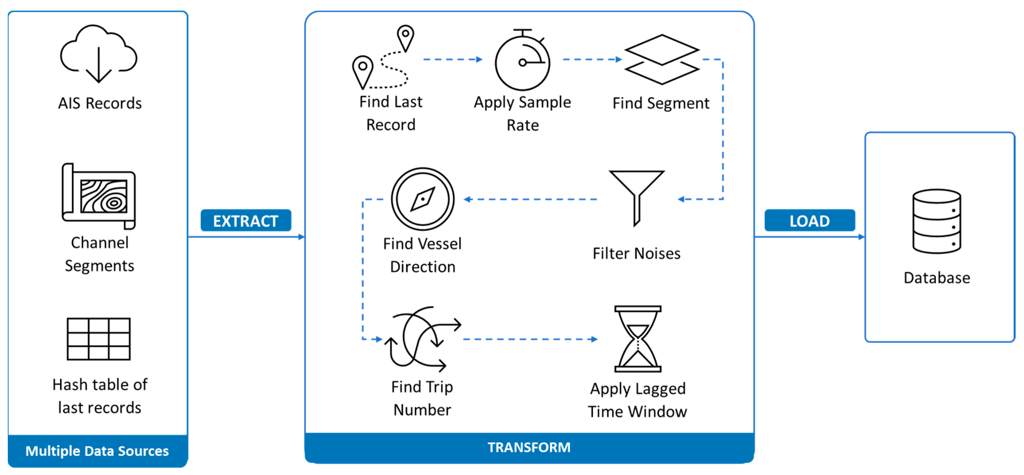
We consider an Extract, Transform, Load (ETL) pipeline to deal with the extraction of the stream of AIS data, process the data, and load the result into a database as depicted in Figure 2. Not only does this procedure help to build customized and useful information to be used instead of raw AIS data but it also helps in making online predictions of vessel movements; it is a big help for the port authorities to know the estimated location of the vessels in a real-time manner when facing a disconnection or a vessel intentionally switch off its location. To do the prediction, some traditional methods and deep learning methods are implemented, and the error of each method has been evaluated. In the following, every component of the ETL pipeline is explained in detail.

3.1. Extracting Data

The first step of the ETL pipeline starts by extracting data from an external source of AIS data. Practically, the stream of real-time data would be provided through APIs. To testify to the proposed method’s functionality in real-world cases, we collected historical data for North America and simulated an API that generates AIS messages in a given time interval. The retrieved data are then filtered based on a specific boundary called the Area of Interest (AoI) to extract only the relevant portions of interest. After filtering, the code performs a data-cleaning process by removing any incomplete or null values. This ensures that the data are accurate and suitable for further analysis or processing. The final result of the code is a cleaned dataset containing the essential and valid data, ready to be used for the Transformation step.

3.2. Transforming Data

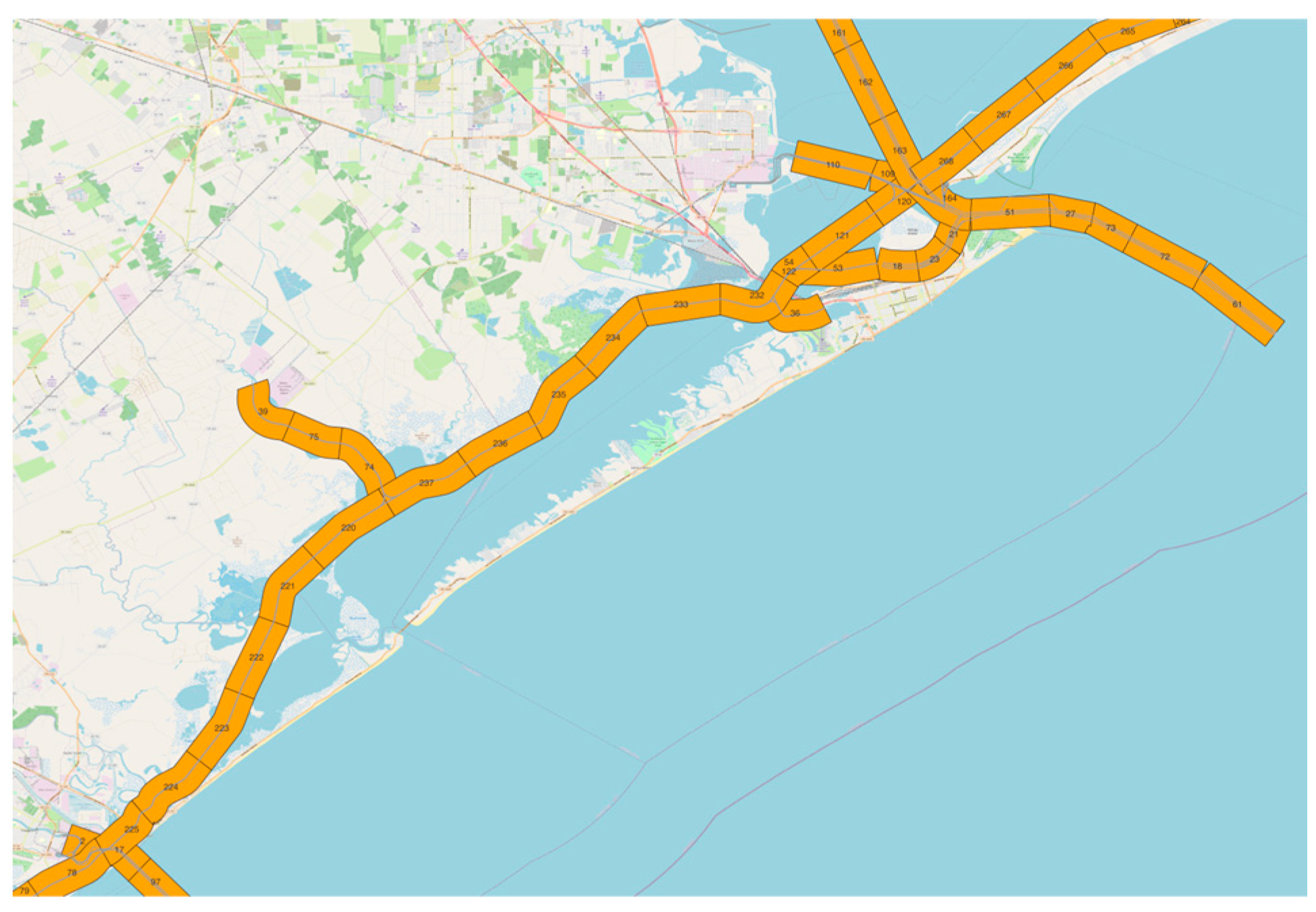
The second component of the ETL procedure is the “Transform”. This step considers the output we have gathered as clean raw AIS data from the Extract part as an input for further processing. The other input is a geographical information system (GIS) layer of all waterways located in the AoI. Thanks to the QGIS toolbox, we employ the “split line to maximum length” function to split the GIS layer into smaller, equally sized segments as depicted in Figure 3. Then a series of functions have been applied to the input data to transform the raw AIS data. The following sections talk about these functions in detail.

• Step 1: Finding the last record

The algorithm is developed based on a hash table, which stores the latest record of each vessel’s data. As the algorithm receives a stream of data; it compares each vessel’s record with the last record already stored in the hash table to compute features such as the time and space distance between a pair of consecutive points. The calculated features will be used in the next steps. If there is no record in the hash table, the algorithm stores the new data as the last record. However, if the vessel’s information is already stored, the algorithm updates the existing data with the newly received data. This allows the algorithm to progressively calculate and update the calculated values in real time, ensuring the latest information is stored and processed accurately.

• Step 2: Applying the sample rate

The other inputs of the transform algorithm are the minimum and maximum acceptable time difference between two consecutive records collected for a vessel. Assuming Δt is a time difference between each vessel’s AIS record and the previous record, the algorithm keeps records only when Δt is between the minimum and maximum time difference. It drops redundant information and breaks the sequence of the AIS records if there is a long pause. Our assumption is to set the minimum acceptable time difference at 5 min and the maximum acceptable time difference at 120 min (2 h).

• Step 3: Finding segments

This step takes the intersection of each AIS record and the pre-defined segments of the AoI to assign the segment’s ids to the records. this helps us summarize the data for each segment and calculate some traffic features like traffic density. Additionally, it drops any records located outside of the segments.

• Step 4: Filtering noises

Trajectory trackers sometimes may generate wrong records that appear as noises in a sequence of locations. To capture and drop such records, we add this step to our transformer. This step uses Δt and Δl—that is, the distance between each record and the previous record—to calculate the average speed. If the average speed is not in a rational range of the vessel’s speed, from 0 to 30 knots, it drops the record.

• Step 5: Determining the vessel’s direction

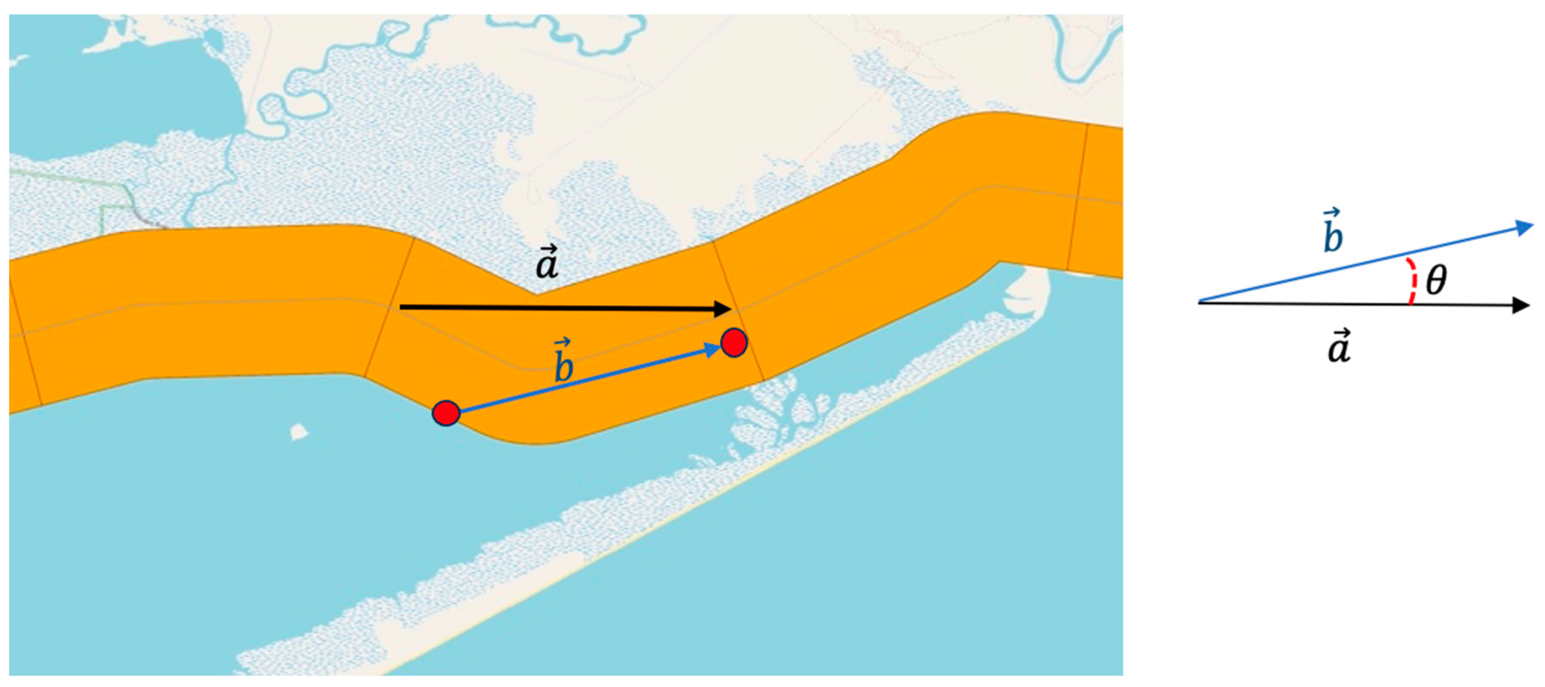
To define the vessel’s direction, we first define the unit vector of the segments’ centerline. As Figure 4 shows, we keep the first and last point of each segment centerline and create a segment vector $\overrightarrow{\mathrm{a}}$. Next, we consider vector b as the distance difference between the new record and the previous record for each vessel. Finally, we utilize the inner product, Equation (1), to calculate the angle between these two arrows:

$$\mathrm{a}·\mathrm{b}=\left|\mathrm{a}\right| \left|\mathrm{b}\right|\cos (\mathsf{\theta })$$

(1)

• where
• a: segment centerline vector
• b: vessel’s movement vector

These two vectors (a, b) make an angle, θ. Based on Equation (1), we have the following:

$$\left\{\begin{array}{lll}0<\mathrm{\theta }\le 90& \mathrm{i}\mathrm{f}& \mathrm{a}·\mathrm{b}>0\\ 270<\mathrm{\theta }\le 360& \mathrm{i}\mathrm{f}& \mathrm{a}·\mathrm{b}>0\\ 90<\mathrm{\theta }\le 270& \mathrm{i}\mathrm{f}& \mathrm{a}·\mathrm{b}<0\end{array}\right.$$

(2)

Therefore, if the inner product of two vectors has a positive value, it means that the $\cos \mathsf{\theta }$ is a positive value, which means we can interpret the two vectors as having the same direction, and we consider it as the “inbound” direction, while if $\cos \mathsf{\theta }$ is a negative value, the direction of the vessel is in the opposite direction of the segment vector, so the vessel’s direction is “outbound”. The example, shown in Figure 3, is an inbound trip because the inner product of (a, b) is a positive value and the $\mathsf{\theta }$ between them is simply between 0 and 90 degrees. This method requires all segment unit vectors to be organized in the head-to-tail position. We use the QGIS toolbox to order segments and find each segment unit vector. We also assume the vessel’s direction is zero when its speed is below 2 knots. Therefore, we define three directions based on the vessel’s speed, the inner product of the vessel’s movement vector, and the segment vector as listed in

Table 2. Direction Values.

Vessel Status	Inbound	Stop	Outbound
Direction value	1	0	−1

.

• Step 6: Determining the Trip Number

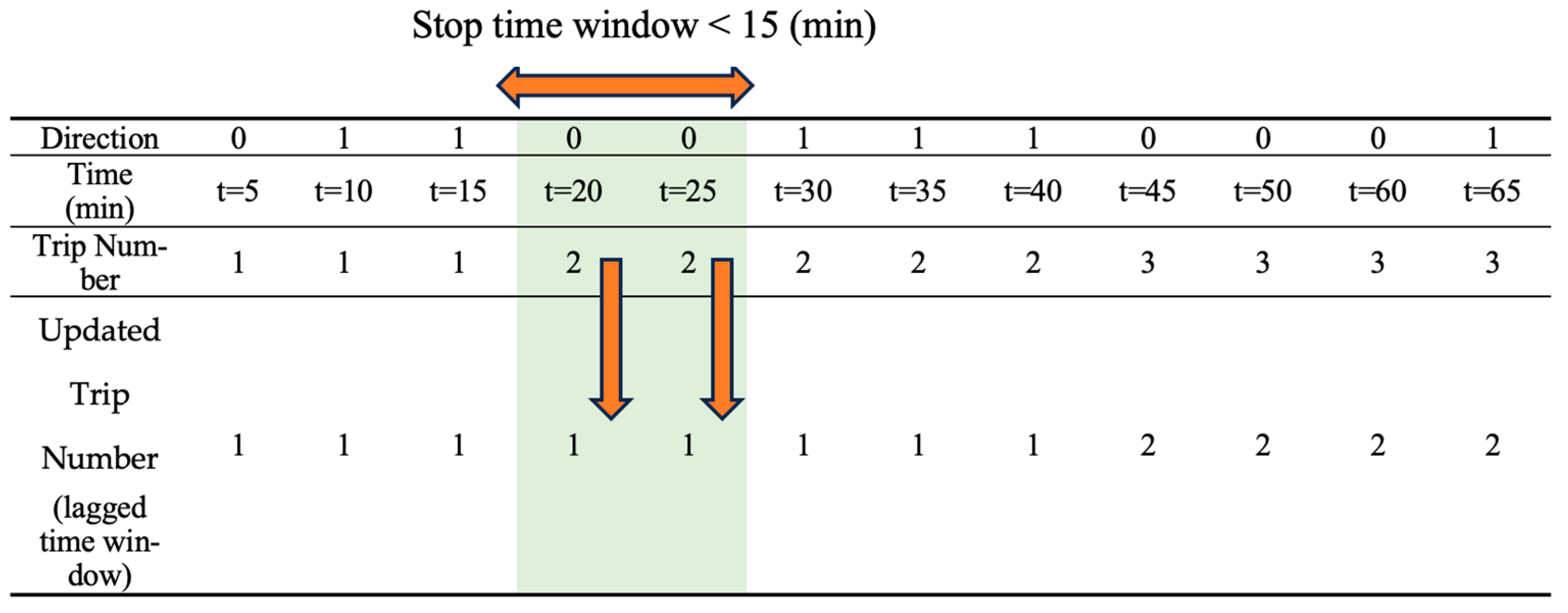
The proposed algorithm aims to determine trip numbers, considering every stop-to-stop interval as a separate trip. To determine the trip number, the code first checks if the new record’s direction is “stopped” and differs from the previous record’s direction. If this condition is met, it implies the start of a new trip. The code increments the trip number by one, assigning it as the previous record’s trip number plus one.

In instances where vessels initiate a trip and make stops during the journey, the algorithm tends to designate each stop as a new trip number, even if the vessel halts briefly and does not signify the initiation of a new trip. To address this, time-lagged windows have been implemented. For trips in which vessels stop during the journey, if the stop time is below a predefined threshold, the algorithm disregards the stop status, considering the trip number as the previous trip number and not initializing it as a new trip. Consequently, the algorithm updates the last vessel’s recorded trip number with a delay, ensuring that the stop status of the vessel is deemed negligible. For more clarification, in Figure 5, we have a record from an MMSI every five minutes, and the algorithm considers each stop to stop as a single trip. Therefore, before using a time-lagged window, the trip number for this specific vessel can increase to three, while in the movement of the vessel, it stops for about 5 min. If we predefine our threshold at 15 min, based on the time-lagged window, we must ignore the stop status and consider it to be the previous trip number. In this case, we have two trip numbers, since at the third stop, the vessel does not stay less than 15 min. Therefore, we initiate a new trip number.

3.3. Load the Processed Data

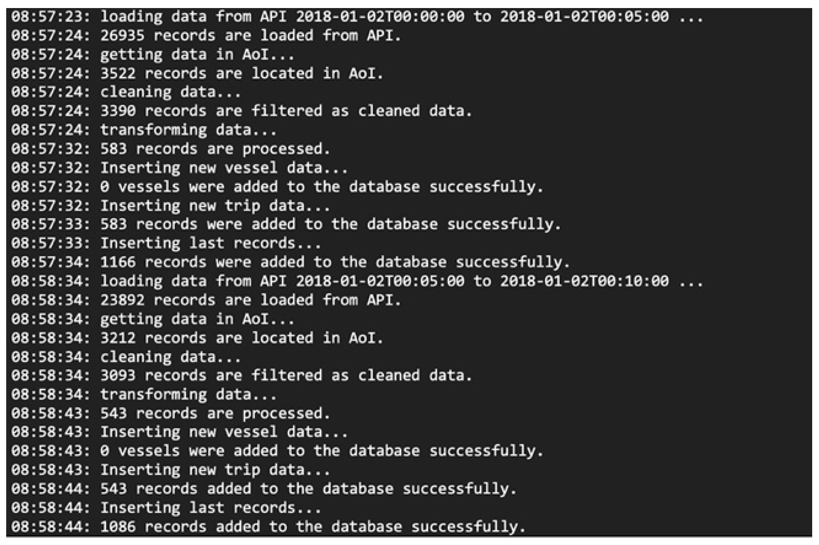
The final stage of the ETL pipeline involves the loading of processed data from the preceding section into a database. We have developed a comprehensive database to store the processed data obtained from the ETL pipeline output. This database incorporates a combination of static and dynamic tables to effectively organize the data. The static tables encompass vessel profile, segments, vessel status, and vessel type. On the other hand, the dynamic tables consist of trips and the last records, which are used for efficient tracking and analysis. As mentioned above, we developed a simulated API to replicate real-world operations of receiving a stream of AIS records. The API uses actual AIS data from 2018 to 2022 but releases them in 5 min time intervals. Then, we connect our pipeline to this API and set it running for all data. Figure 6 shows the log message when running the pipeline. As shown in log messages, the pipeline is highly efficient so that it can process 26,000 records in 10 s and compress them into 583 records.

3.4. Trajectory Prediction

This section discusses two distinct approaches used for predicting vessels’ trajectories. The first method is a traditional approach. In contrast, the second approach involves utilizing a sequence-to-sequence recurrent neural network model (RNN).

3.4.1. Dead Reckoning

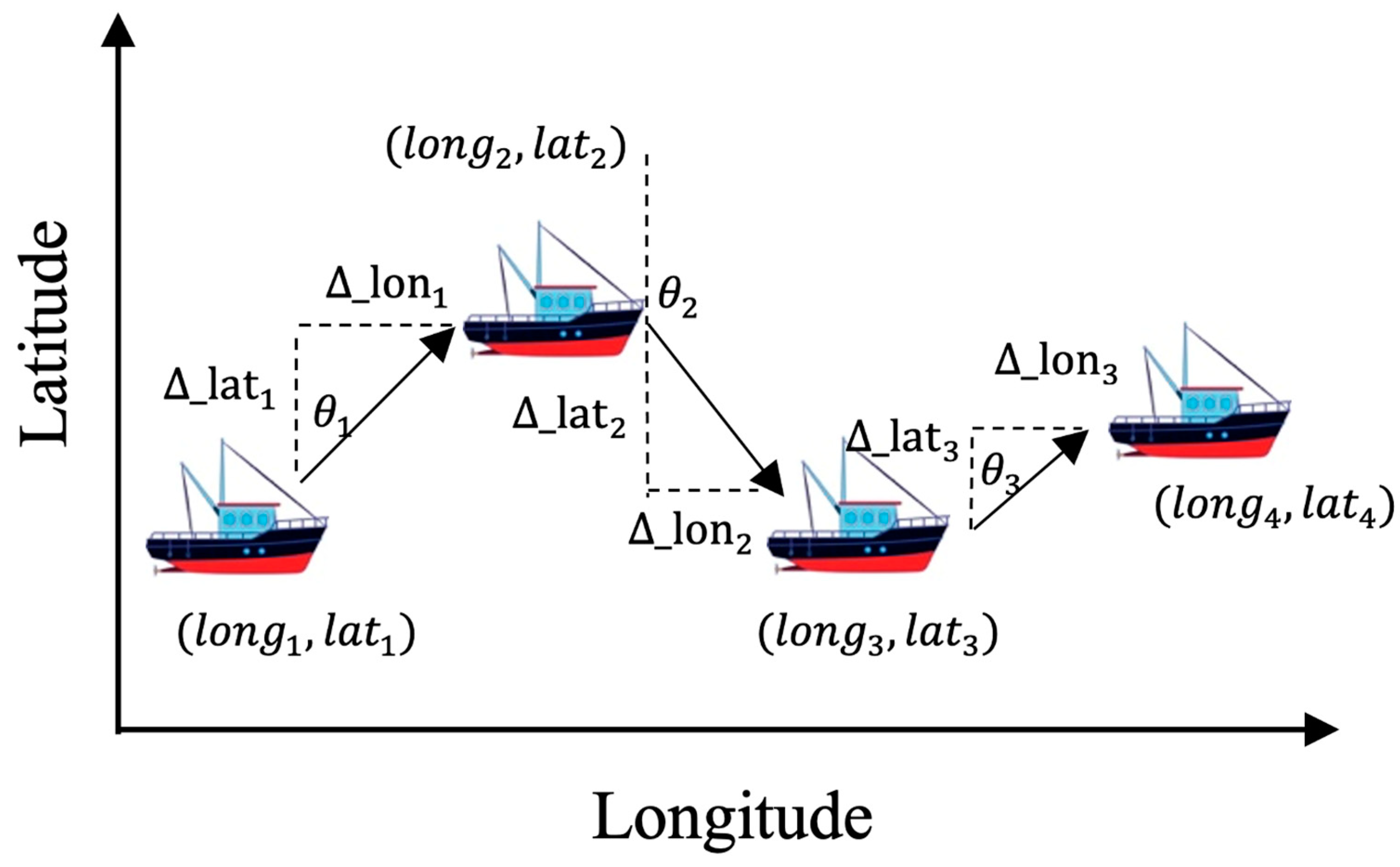
In the realm of vessel navigation, a traditional prediction method known as dead reckoning is employed to estimate the next position in a series of trajectory data using current and previous records. Dead reckoning allows us to estimate the next location of the vessel based on its past movements, even when real-time data, such as AIS data, are unavailable or disrupted. There are two scenarios in which dead reckoning comes into play. In Scenario I, we utilize the speed and course over ground obtained from the AIS record as an input to predict its next location. On the other hand, in Scenario II, we rely on the pre-record location of the vessel to find its next location. By extrapolating the vessel’s historical data, we can project its next position, assuming it maintains a consistent speed. To facilitate this prediction process, we undertake the following steps:

• Step 1. Preparing the inputs

To streamline the process, we retrieve relevant data from the database. In the trip table, we introduce two additional columns that showcase the pre-record and next-record locations of the vessels.

• Step 2. Dead reckoning method

Assuming our aim is to obtain predictions for each specific time interval, we apply Equation (3) to calculate the distance traveled by the vessel within the defined time interval, which is assumed to be 5 min (0.083 h). Regarding [34], in Equation (4) the angular distance is calculated by dividing the linear distance by the earth’s radius. In Equation (5), the latitude of the next point is calculated. To find the longitude of the next point, first we should calculate the projected latitude difference in Equation (6). The ratio n in Equation (7) is introduced to account for the fact that, as the vessel moves along a rhumb line, the meridional scale (change in latitude) is not equal to the zonal scale (change in longitude) due to the convergence of meridians toward the poles. Therefore, the term n is used to adjust for the variation in the size of a degree of the longitude with the latitude. We have the longitude difference and the longitude of the next point in Equations (8) and (9), respectively.

$$\mathrm{d}=1.15 \mathrm{s}·{∆}_t$$

(3)

$$\delta =\mathrm{d}/\mathrm{R}$$

(4)

$${\phi }_2={\phi }_1+\delta ·\cos \left(\mathsf{\theta }\right)$$

(5)

$$∆\psi =\ln (\mathit{tan}\left(\pi /4+{\phi }_2/2\right)/\mathit{tan}\left(\pi /4+{\phi }_1/2\right)$$

(6)

$$\mathrm{n}=∆\phi /∆\psi$$

(7)

$$∆\lambda =\delta ·\mathit{sin}(\mathsf{\theta })/\mathrm{n}$$

(8)

$${\lambda }_2={\lambda }_1+∆\lambda$$

(9)

• where
• d: distance in mile
• s: vessel’s current speed in knots
• ${∆}_t$: given time interval (5 min = 0.083 h)
• R: earth’s radius in miles (3958.80 miles)
• $\mathsf{\theta }$: vessel’s course over ground
• ${\phi }_1$: latitude of current point
• ${\phi }_2$: latitude of next point
• $∆\phi$: latitude difference
• $∆\psi$: projected latitude difference
• n: adjustment ratio for the variation in the size of a degree of longitude with latitude
• $∆\lambda$: longitude difference
• ${\lambda }_1$: longitude of current point
• ${\lambda }_2$: longitude of next point
• ${\phi }_0$: latitude of previous point
• ${\lambda }_0$: longitude of previous point

In scenario II, instead of using the course over the ground, as recorded in the AIS data, we calculate it by comparing the current record and the previous one. Figure 7 shows the dead reckoning method for finding the next location of the vessel using the pre-record and the new record.

3.4.2. RNN Method

The sequence-to-sequence recurrent neural network (RNN) method is a more advanced approach for predicting the vessel’s next timestamp location. This technique leverages the power of deep learning to model sequential data effectively. The RNN architecture is designed to handle sequential input data, such as a vessel’s position and timestamp over time. It is capable of capturing temporal dependencies and learning complex patterns from the historical trajectory of the vessel. However, standard RNNs have limitations in capturing long-term dependencies, making them less suitable for tasks requiring long-term memory [1]. Long Short-Term Memory (LSTM) is a powerful variant of RNNs that addresses the challenges of capturing long-term dependencies in sequential data, making it well-suited for tasks that require modeling complex sequential patterns, such as sequence-to-sequence learning and natural language processing.

3.4.3. LSTM Structure

LSTM is a type of recurrent neural network (RNN) architecture designed to address the vanishing gradient problem and capture long-term dependencies in sequential data. It is particularly effective in tasks involving sequences, such as time series prediction and natural language processing. The components include the following:

• Input Gate: Determines which information from the current input should be stored in the cell state;
• Forget Gate: Controls what information should be discarded from the cell state;
• Cell State updates: Maintains the long-term memory information;
• Output Gate: Determines the next hidden state based on the cell state.

3.4.4. Sequence-to-Sequence Model

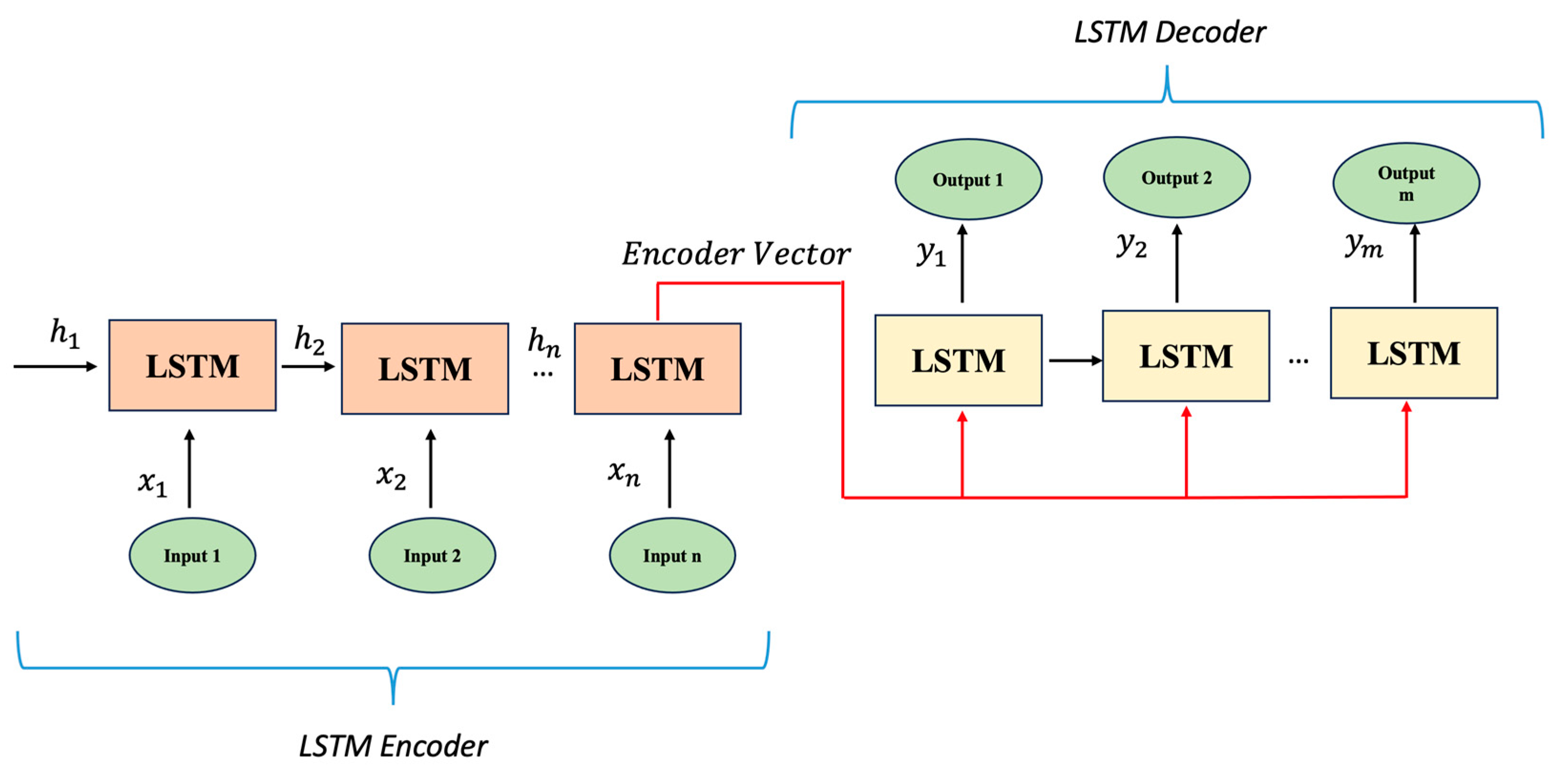
A sequence-to-sequence (Seq2Seq) model (Figure 8) is designed for tasks where the input and output are both sequences of varying lengths. Common applications include machine translation and text summarization. The components include the following:

• Encoder: Processes the input sequence and encodes it into a fixed-size context vector;
• Decoder: Generates the output sequence based on the context vector produced by the encoder.

In our case, we use different lengths to predict the points, so we use a Seq2Seq structure, which is structured as below:

• Step 1: Preparing the inputs;
  • First, we call processed AIS data from the database and store it as a dataset.
• Step 2: Feature selection and normalization.

Vessel latitude and longitude coordinates are essential for capturing the vessel’s movement patterns. Therefore, we use these two features as the input for the Seq2Seq model. Additionally, as shown in

Table 3. X and Y features.

Features	Speed over Ground	Course over Ground	Vessel Heading	Longitude	Latitude
X features	✓	✓	✓	✓	✓
Y features				✓	✓

, we add the vessel’s speed over the ground, the course over the ground, and the heading independent variables. Then we perform data normalization on the selected columns to bring them to a similar scale. This is crucial for ensuring that the LSTM model can effectively learn from the data and avoid numerical instabilities during training.

• Step 3: Converting data into tensors.

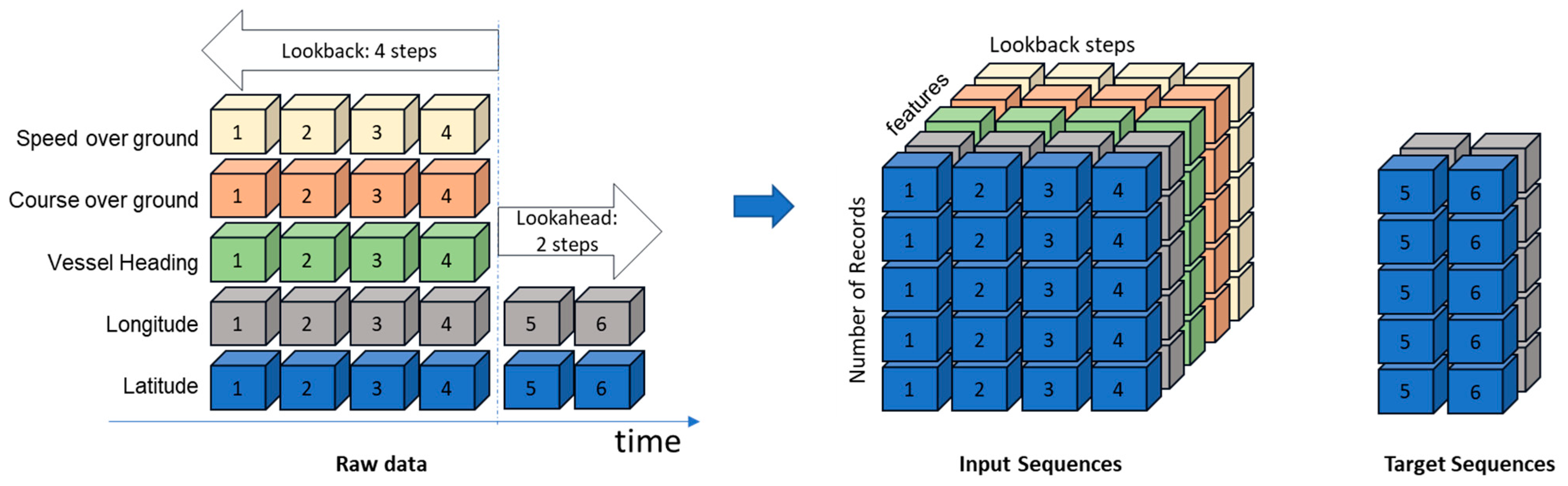
A sliding window method is applied to convert data tables into a three-dimensional matrix tensor. Figure 9 illustrates how the sequences, and their corresponding target values, have been selected. The output of this step is x and y tensors, which are the input sequence (here this is four sequences) and target sequence (here this is two sequences), respectively.

• Step 4: Training the Seq2Seq model.

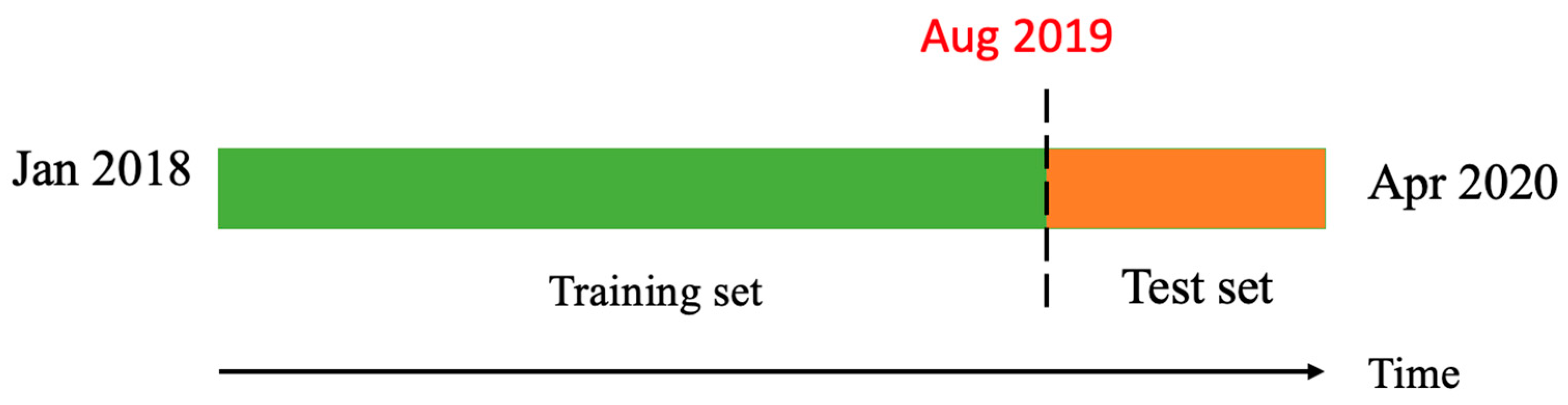
We split the data into 80% training and 20% validation sets. This operation does not require data shuffling and sorts data based on the record date and time to choose the first 80 percent of the data as the training dataset. As depicted in Figure 10, three years of data from January 2018 to April 2020 is selected and based on the chronological split, 80% of the data falls between Jan 2018 and Aug 2019.

• Step 5: Seq2Seq model architecture.

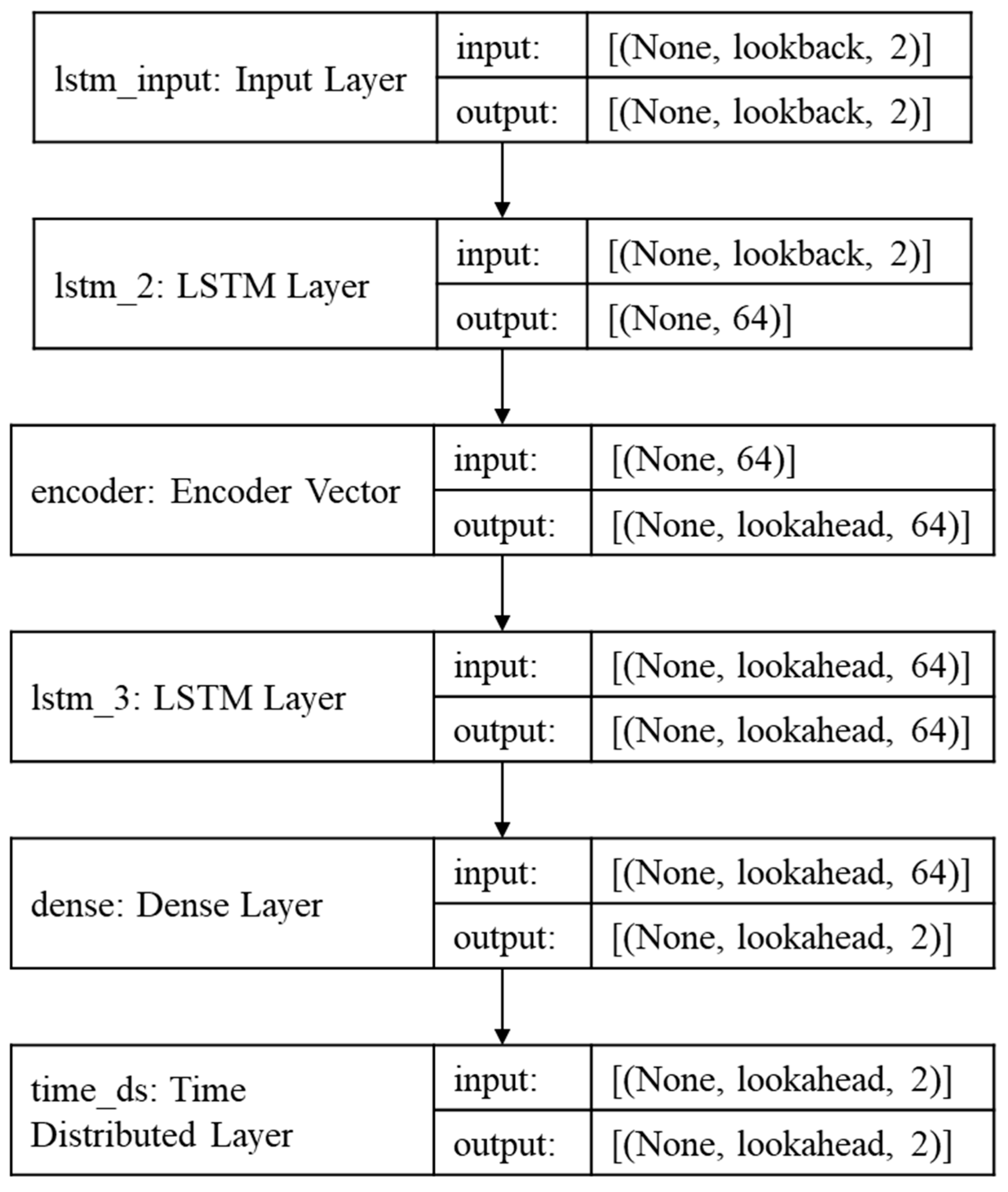
In the context discussed in Section 3.4.4, where input and target sequences vary in length, the model architecture, as illustrated in Figure 8, has been tailored accordingly. To accommodate diverse configurations for sensitivity analysis, the generalized format is presented in Figure 11. Using TensorFlow, we create a sequence model with 50 epochs and 64 hidden layers. The goal is to predict the vessel’s trajectory based on historical data using this model. The initial step involves selecting the input to the model with a specified lookback value of 5, where 5 denotes the number of features in the X dataset. This input is then fed into the LSTM layer, producing an output with a hidden layer of 64 units and a repeated vector, also known as the encoder vector. This fixed vector is generated ‘m’ times and serves as the input for the subsequent LSTM layer, utilizing the value (lookahead, 64). Consequently, the final output of the model is represented as a lookahead value of 2, where 2 signifies the number of features in the Y dataset. This architectural design enables the model to effectively handle varying lookback and lookahead values during the sensitivity analysis.

• Step 6: Model evaluation.
  • In order to evaluate the model performance, the following metrics are defined:
• R2

R-squared measures the proportion of the variance in the dependent variable (the actual next coordinates) that is explained by the independent variable (the predicted next coordinates). It ranges from 0 to 1, where 1 indicates a perfect fit, meaning that the model’s predictions perfectly match the actual data.

$$R^2=1-\frac{\sum _{i=1}^n{\left(y_i-\widetilde{y_i}\right)}^2}{\sum _{i=1}^n{\left(y_i-\overline{y_i}\right)}^2}$$

(10)

• Mean Square Error (MSE)

MSE calculates the average of the squared differences between the predicted and actual values. It penalizes large errors more heavily. A lower MSE indicates that the model’s predictions are closer to the actual values.

$$MSE=\frac{1}{n\sum _{i=1}^n{(y_i-\widetilde{y_i})}^2 }$$

(11)

• Mean Absolute Error (MAE)

MAE calculates the average of the absolute differences between the predicted and actual values. It provides a measure of the average magnitude of errors.

$$MAE=\frac{1}{n}\left|(y_i-\widetilde{y_i})\right|$$

(12)

• Mean Absolute Percentage Error (MAPE)

Aside from the conventional metrics, we calculate the distance between the predicted and actual coordination in miles and feet and take the average of the distance of all the predicted points.

$$MAPE=\frac{1}{n} \sum _{i=1}^n\left|\frac{(y_i-\widetilde{y_i})}{y_i}\right|\times 100$$

(13)

• Mean offset from Centerline (MFC)

We determine the mean offset from the channel centerline by measuring the distance between the predicted points and the centerline of the channel and then calculating the average of these distances. This helps us to have a better estimation of our model if it is predicting the point in the land rather than the waterway. The red circles in Figure 12 are predicted points and the dashed line is the centerline of the channel.

$$MFC=\frac{1}{n}\left|\overrightarrow{r}\right|· \sin (\mathsf{\theta })$$

(14)

4. Application

4.1. User Interface Dashboard

The proposed algorithm has been deployed for implementation in the Texas coastal lines region, specifically targeting the GIWW (Gulf Intracoastal Waterway). As part of the implementation, we simulate a continuous stream of AIS data from 2018. These data are then processed using an ETL pipeline and stored in a database. To provide an intuitive user interface, we have designed a dashboard that allows end users to retrieve the data they need. The dashboard initially displays real-time vessel traffic, as shown in Figure 13. In addition to real-time data, the dashboard provides access to historical information. Users can query various metrics such as traffic flow, dwell time, OD matrix, trip generation, trip attraction, and individual vessel trips. These queries can be filtered based on the vessel type and specific date ranges.

4.2. Data Processing Efficiency

The proposed ETL pipeline is highly efficient, processing data at a rate of 0.000001 s per record. For example, if we want to process ten million records, it will take just ten seconds using our algorithm. The speed of this method represents a notable advancement compared to traditional data processing. It allows for real-time monitoring of vessel traffic efficiently. Additionally, the ETL has been tested on a simulated environment and can work simultaneously with the current AIS collection systems. As a result, it does not require a high-end computer to process raw AIS data because it processes a chunk of the most recent data at each iteration.

4.3. Prediction Evaluation

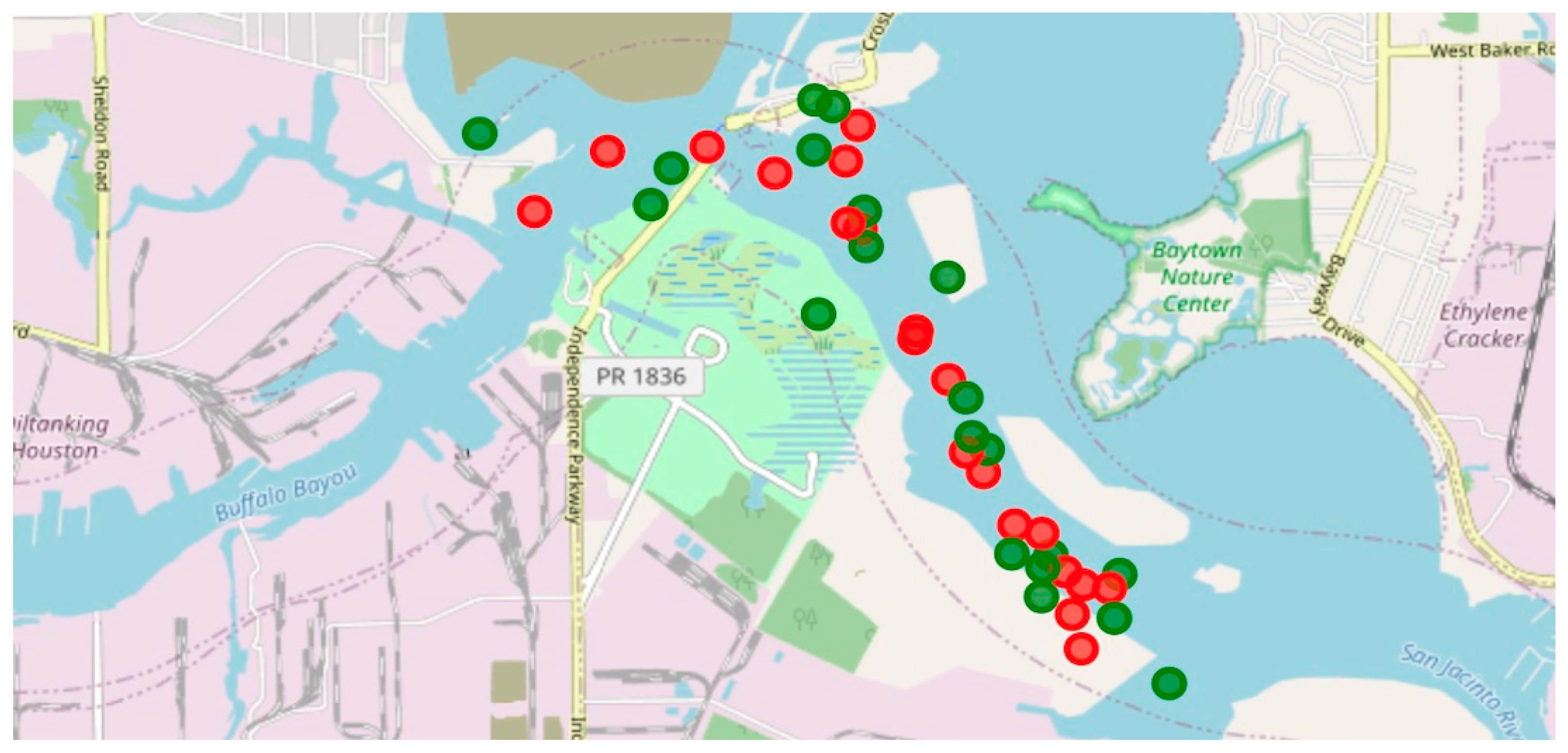
As discussed, in the previous section, the dead reckoning method and LSTM algorithms have been implemented to predict the next location of the vessel’s movement. To visualize the prediction of both methods, we use the folium library in Python. The real location and the predicted location of a single vessel using the dead reckoning II method are depicted in red and green colors, respectively, in Figure 14.

To evaluate the method in Scenarios I and II, the mean offset and other model evaluation metrics have been investigated, and the result is shown in

Table 4. Model evaluation results.

Metrics	Dead Reckoning I	Dead Reckoning II	Seq2Seq
r square	0.9996	0.9999	0.9999
mean absolute error	0.0111	0.0032	0.0028
mean square error	0.0149	0.0064	0.0046
mean absolute percent error (%)	2.3	0.68	0.59
mean offset (mile)	1.03	0.32	0.28
mean offset (ft)	5433	1674	1454
mean offset from centerline(mile)	---	---	0.12

. While the traditional method may be simple to implement, it may not capture complex patterns or account for irregularities in the vessel’s movement. Additionally, the first two approaches can only predict one location ahead of time, and they are not able to predict more than one step in the future. They also may not perform well in situations where the vessel’s trajectory is subject to sudden changes or nonlinear behavior.

4.4. Sensitivity Analysis

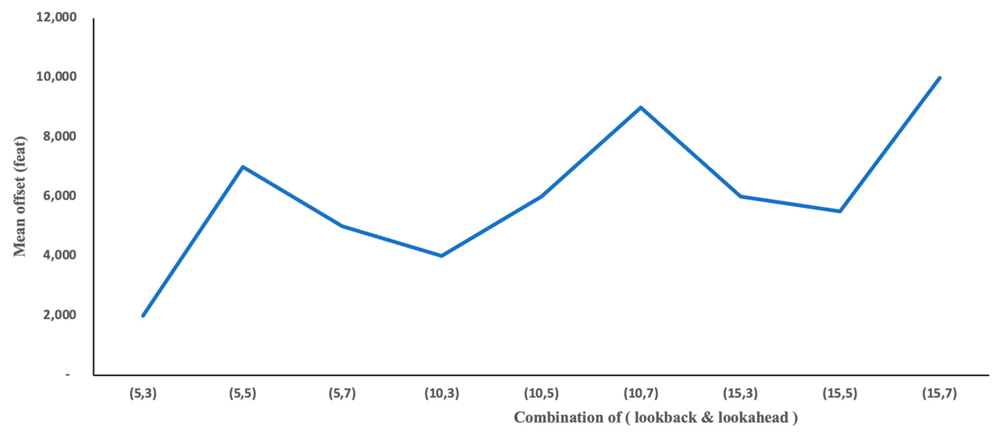
To gain deeper insights into the impact of the input sequence length on the predictions, various values were experimented with for both lookback and lookahead settings. Through a comprehensive analysis of these combinations, it was determined that the optimal configuration for lookback and lookahead is (5, 3) as shown in

Table 5. Sensitivity analysis with different combinations of lookback and lookahead.

Mean Offset (mile)		Lookahead Window
		3	5	7
Lookback window	5	4.03	4.72	5.25
	10	5.74	6.7	5.94
	15	6.27	7.02	7.86

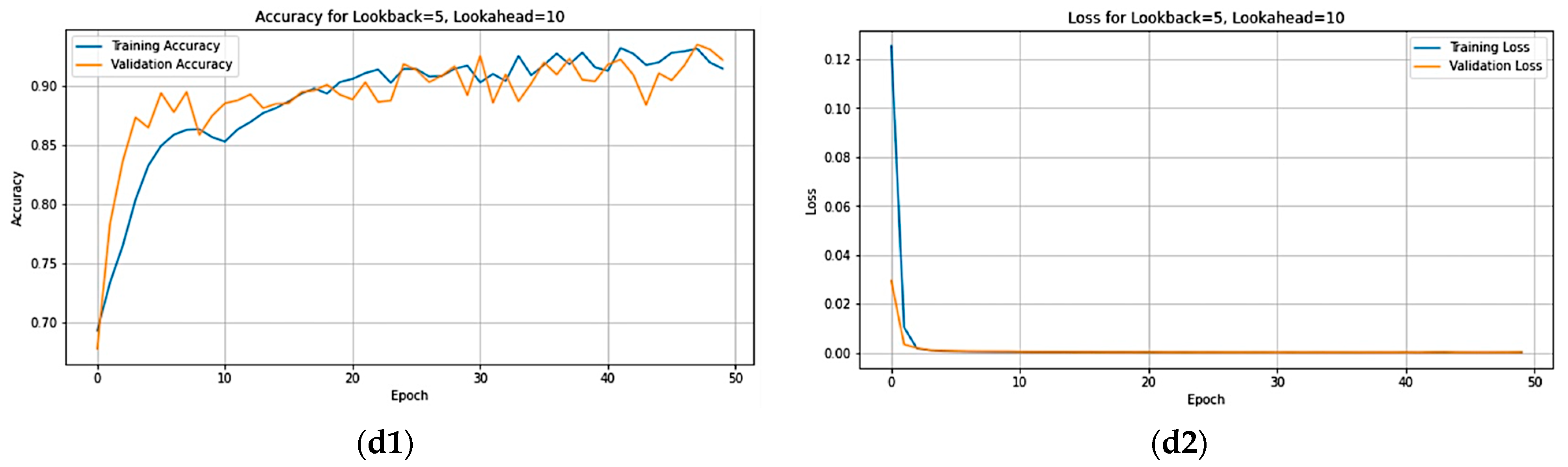
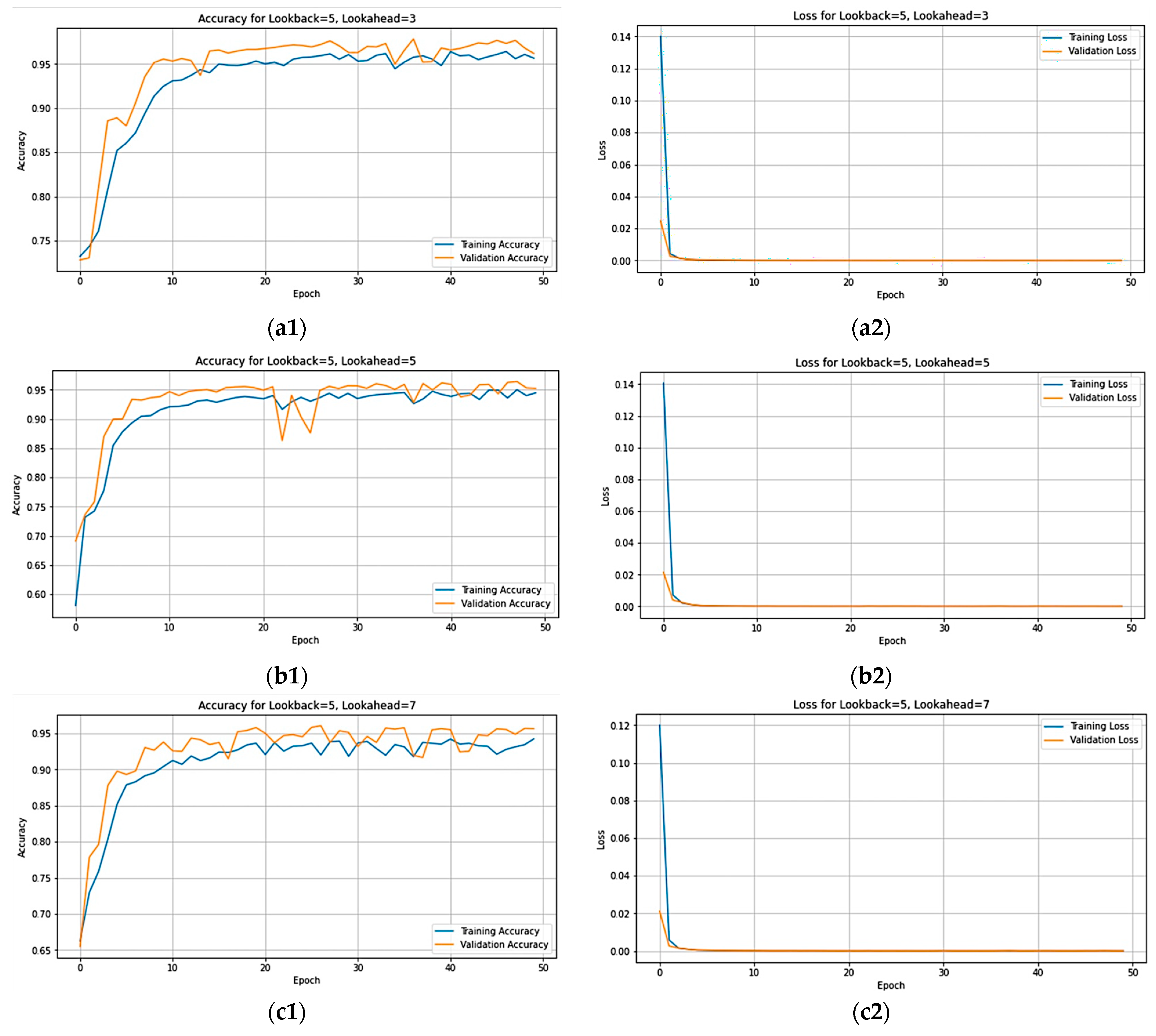
. This signifies that the model exhibits strong predictive performance when provided with five historical records to forecast the subsequent three records. The sensitivity analysis for different combinations of lookback and lookahead values is shown in Figure 15, which denotes that the combination (5, 3) shows better results in terms of the mean distance. Additionally, Figure 16 provides a visual representation of both accuracy and loss per epoch. The graphs on the right illustrate the loss per epoch, showcasing closely aligned training and validation curves, indicating that the model is not overfitting. On the left, the accuracy per epoch plots reveals consistently high values, approaching one, indicative of a positive trend. Notably, the a1 plot exhibits particularly promising results, suggesting that selecting a lookahead of three yields enhanced the accuracy. While other lookahead values display slightly decreased accuracy compared to lookahead three, the overall trend remains favorable. This indicates that opting for lookahead values of five, seven, and ten still maintains a satisfactory level of accuracy without a significant decline.

Note that it was impossible for us to capture weather data and merge them with AIS data based on time and location. Thus, we plotted our model’s error (mile offset between the predicted and actual point) versus the month of prediction to show the weather’s impact on our model’s performance. As shown in Figure 17, there is no pattern in different months.

Obviously, different vessel types show different maneuvers in channels and narrow waterways. Especially in channels that have width or depth limitations and put restrictions on vessels based on their type and dimensions, as shown in Figure 18, tug tows have the lowest error since their operations are hardly impacted by such restrictions. The average offset values of tankers and cargos are also low, which is a good sign, because, in practice, we care more about tankers and cargo’s locations in channels.

In Figure 19, the traffic density of the Galveston port with id segments of 18, 23, and 73 and the Houston ship channel with id segments of 43, 66, and 94 is illustrated.

5. Discussion

Looking forward, the research suggests two important future directions. Firstly, an examination of the system’s feasibility and its applicability to LSTM networks is essential. Evaluating the scalability and adaptability of the proposed framework under different operational conditions, such as high-traffic scenarios and diverse waterway characteristics, will provide valuable insights. Additionally, exploring the integration of advanced machine learning techniques beyond LSTM could enhance predictive capabilities. Secondly, the research lays the groundwork for autonomous vessel systems. The system’s ability to handle false or missing AIS records through dead reckoning and machine learning techniques sets the stage for developing intelligent, self-adjusting vessels. This evolution aligns with industry trends toward autonomy, particularly in navigating narrow waterways and channels, offering a potential solution to the challenges of pilot training and scheduling. Exploring these future directions will not only contribute to academic discourse but also offer practical insights for the ongoing digital transformation of maritime operations.

6. Conclusions

In the realm of maritime tracking systems, current platforms like Marine Traffic, VesselFinder, and AccessAIS serve as vital tools for monitoring vessel movements, providing real-time insights into vessel types, names, and directions. However, these systems face notable limitations, including the absence of detailed historical data and the cumbersome process of downloading raw information, hindering users seeking comprehensive insights. Additionally, these platforms lack features such as traffic information, mooring locations, and advanced predictive capabilities for estimated time of arrival (ETA). Our proposed model addresses these gaps by introducing innovative features and addressing existing drawbacks. Through real-time transformation, the model processes and analyzes data in smaller, more manageable chunks, optimizing time efficiency. Using a 5 min sample rate reduces unnecessary data volume and structures data for storage efficiency by converting repetitive columns into dimension tables. The model also introduces new features, including trip number, direction, travel miles, travel time, segments, and origin/destination, enhancing the depth of analysis. Furthermore, the model addresses issues of noise and missing records, ensuring a more reliable and comprehensive maritime tracking solution.

Our research introduces an inclusive and effective framework for the processing of maritime data, tracking vessel traffic, and predicting their next locations. Through the implementation of an Extract, Transform, and Load (ETL) pipeline, we have successfully processed raw AIS data, augmenting it with additional attributes like vessel direction and trip number. The utilization of an inner product context for defining vessel direction and a time-lagged window for trip estimation has proven highly effective, enabling the accurate processing of millions of data entries within seconds. The newly designed system, which eliminates the necessity for raw AIS data, exhibits the capacity to handle extensive information, rendering it a valuable tool for maritime applications. Processed data are stored in a database, and our user interface offers real-time visualizations of vessel traffic, providing port authorities with effective monitoring capabilities. In the prediction phase, we explored two distinct approaches: the conventional dead reckoning method and a deep learning technique using a decoder-encoder model. Our findings revealed that the second scenario of the dead reckoning method, considering the angle between the pre-record and the new record, resulted in lower prediction errors compared to the course of the ground-based approach. Furthermore, the Seq2Seq model demonstrated promising outcomes in predicting the trajectories of vessels based on historical data. Our algorithm is versatile and applicable to diverse maritime scenarios, offering valuable insights and facilitating improved decision-making processes. For this study, we applied the framework to the Gulf Intracoastal Waterway (GIWW) in the Texas region, simulating AIS APIs. The results underscore the system’s efficiency in processing large amounts of data and achieving precise vessel location predictions.