


Automatic Identification System-Based Prediction of Tanker and Cargo Estimated Time of Arrival in Narrow Waterways


Abstract
1. Introduction
2. Related Works
2.1. Path Finding/Other Methods
2.2. Machine Learning
2.2.1. Road Application
2.2.2. Waterway Application
3. Problem Definition
AIS Data
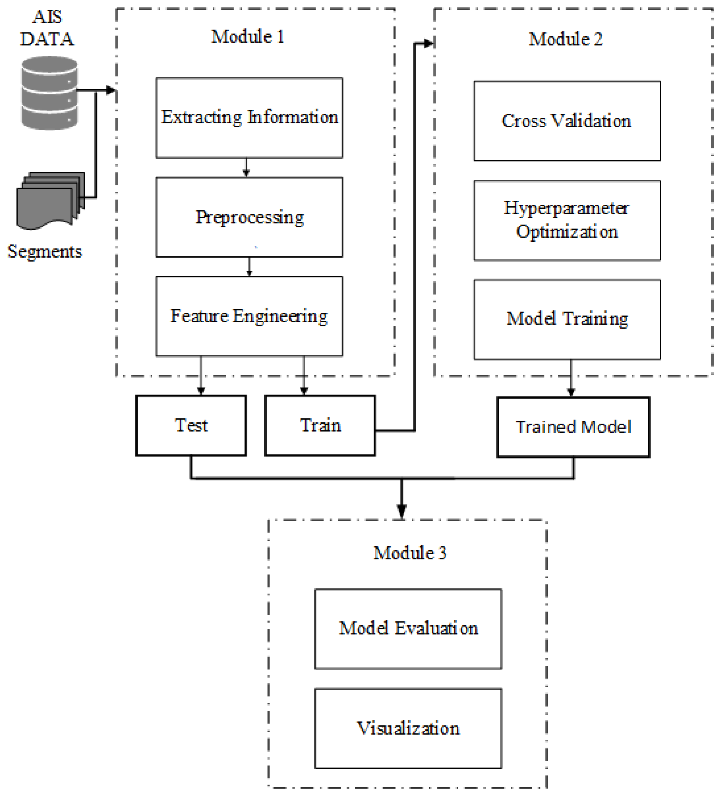
4. Methodology
4.1. Module 1: Preprocessing
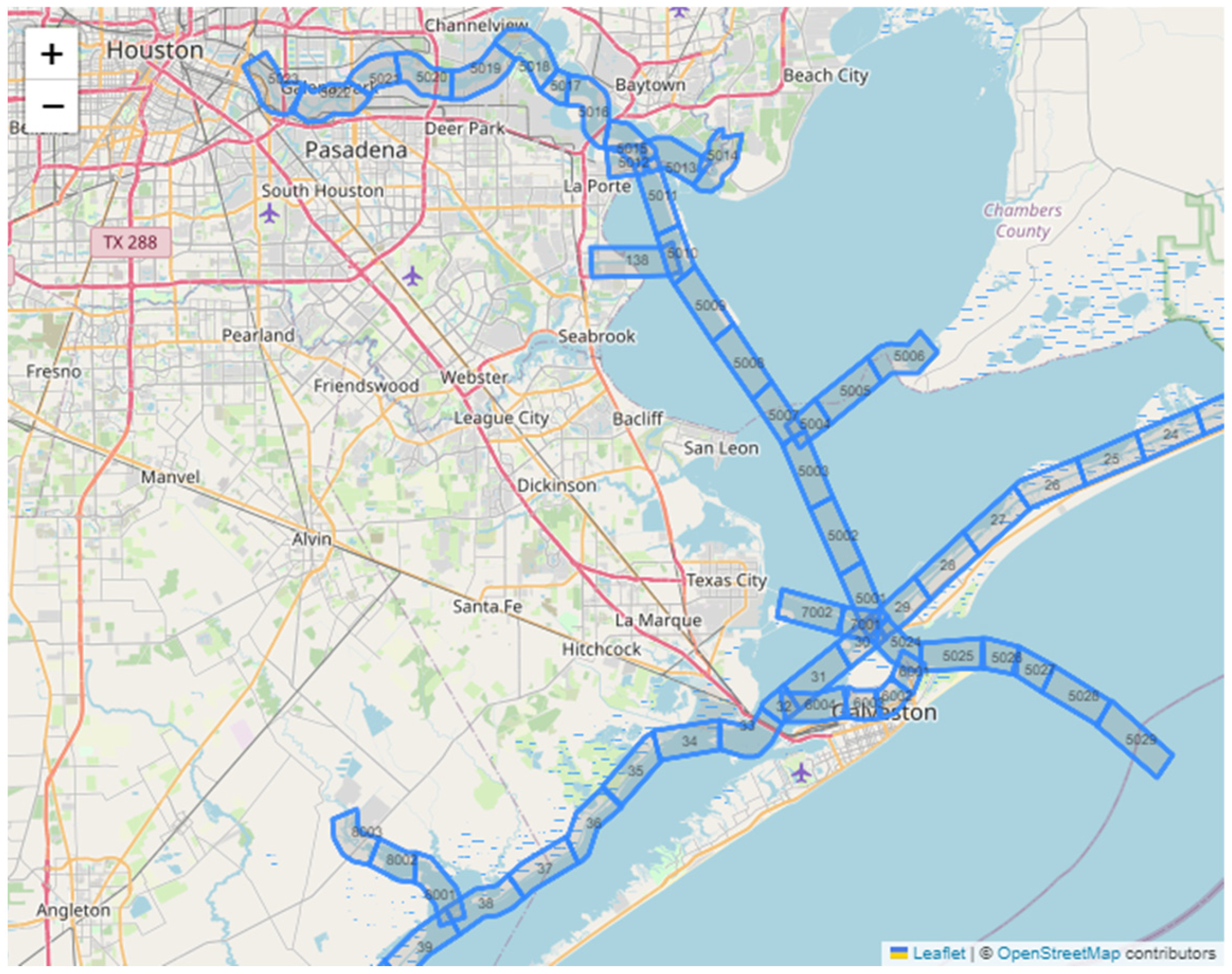
4.1.1. Segmentation of Area of Interest
4.1.2. Extracting Features from Raw AIS Data
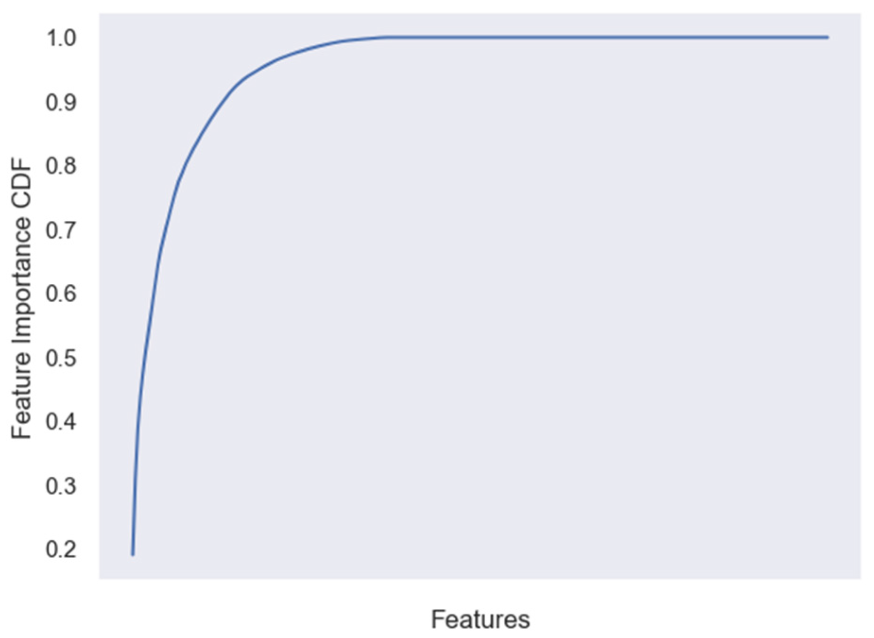
4.1.3. Principal Component Analysis
- is an orthogonal matrix containing the left singular vectors.
- is an diagonal matrix containing the singular values on the diagonal.
- is a orthogonal matrix containing the right singular vectors.
4.1.4. Feature Engineering
Vessel Segments Path
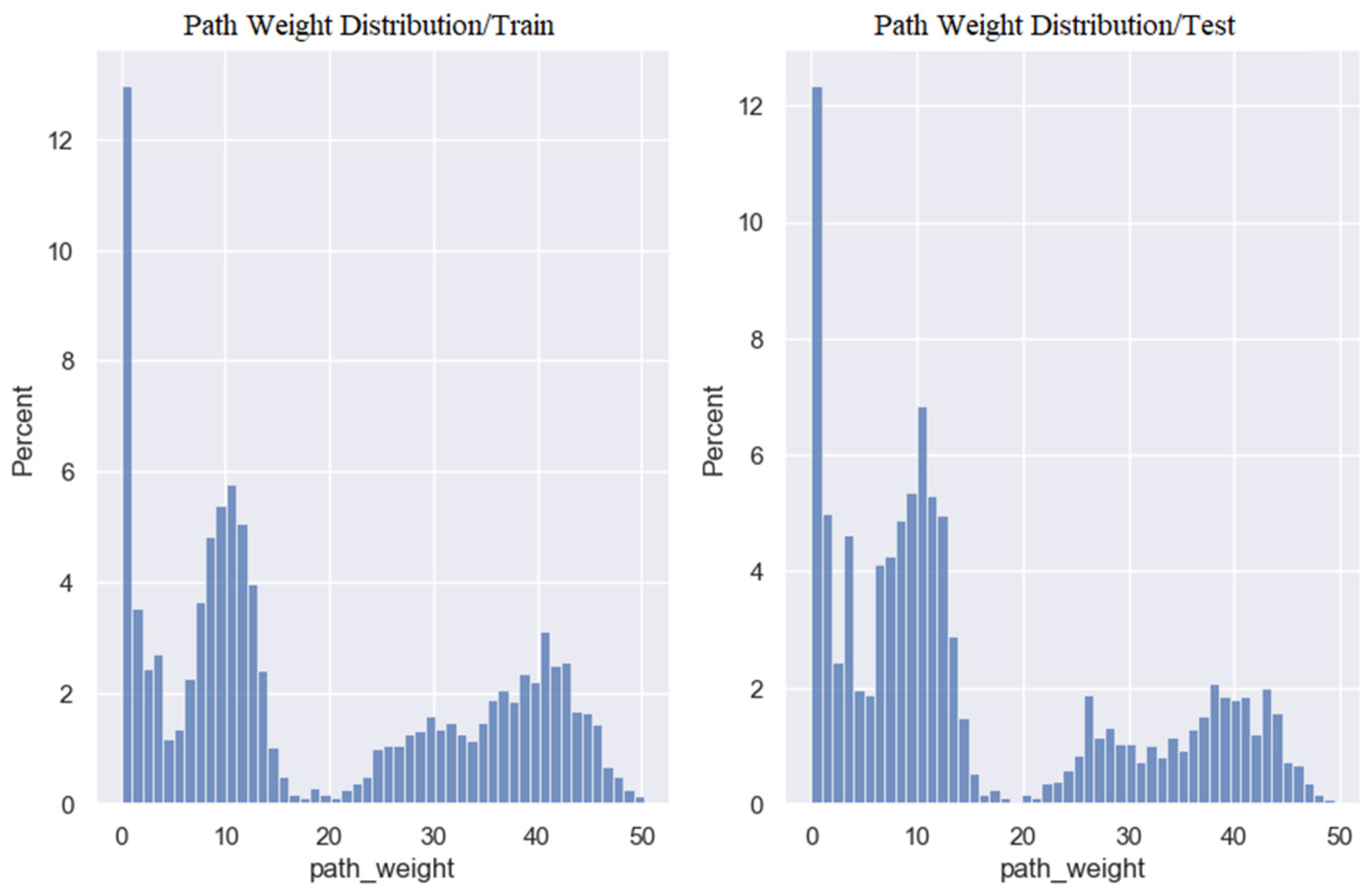
Path Weight
4.2. Module 2: Modeling
Metrics
4.3. Module 3: Apply Model
5. Experimental Study
5.1. Preprocessing Module
5.2. Modeling Module
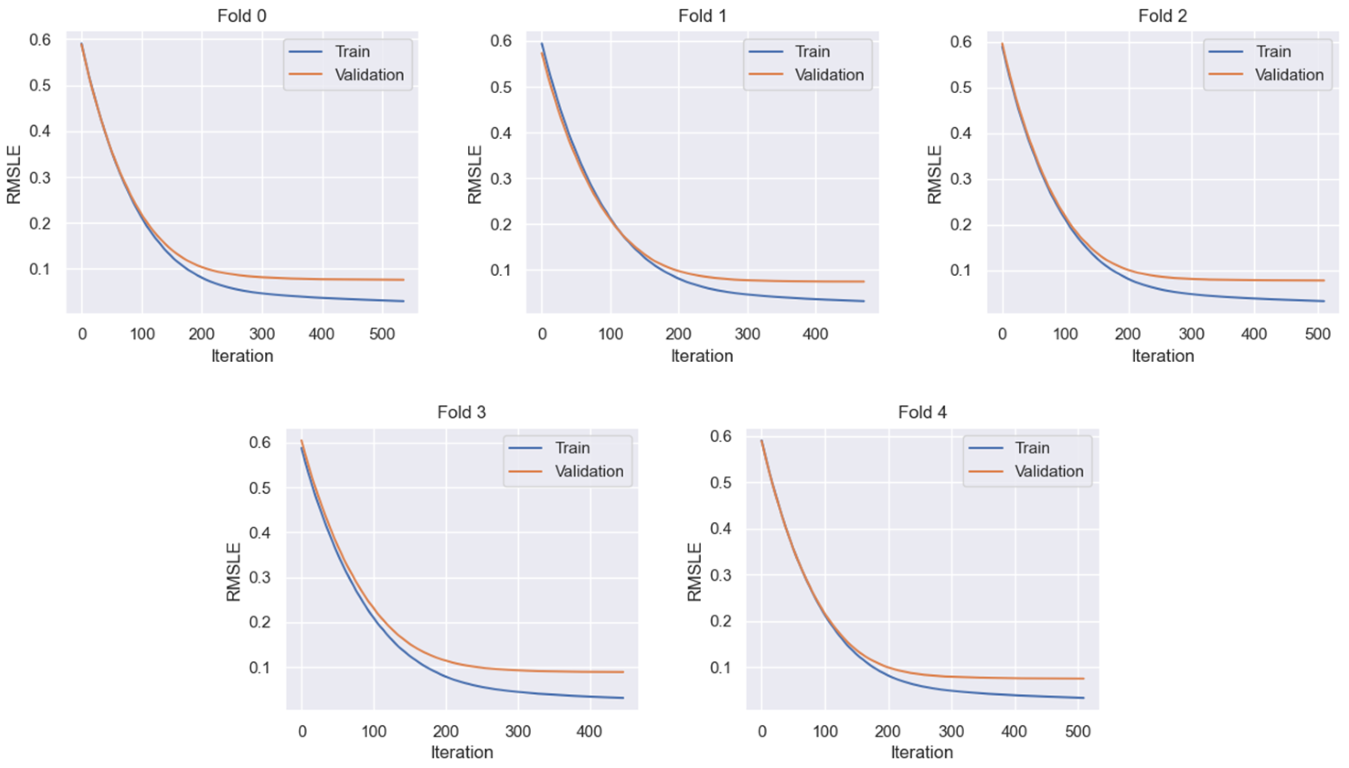
5.2.1. Hyperparameter Optimization
5.2.2. Model Training
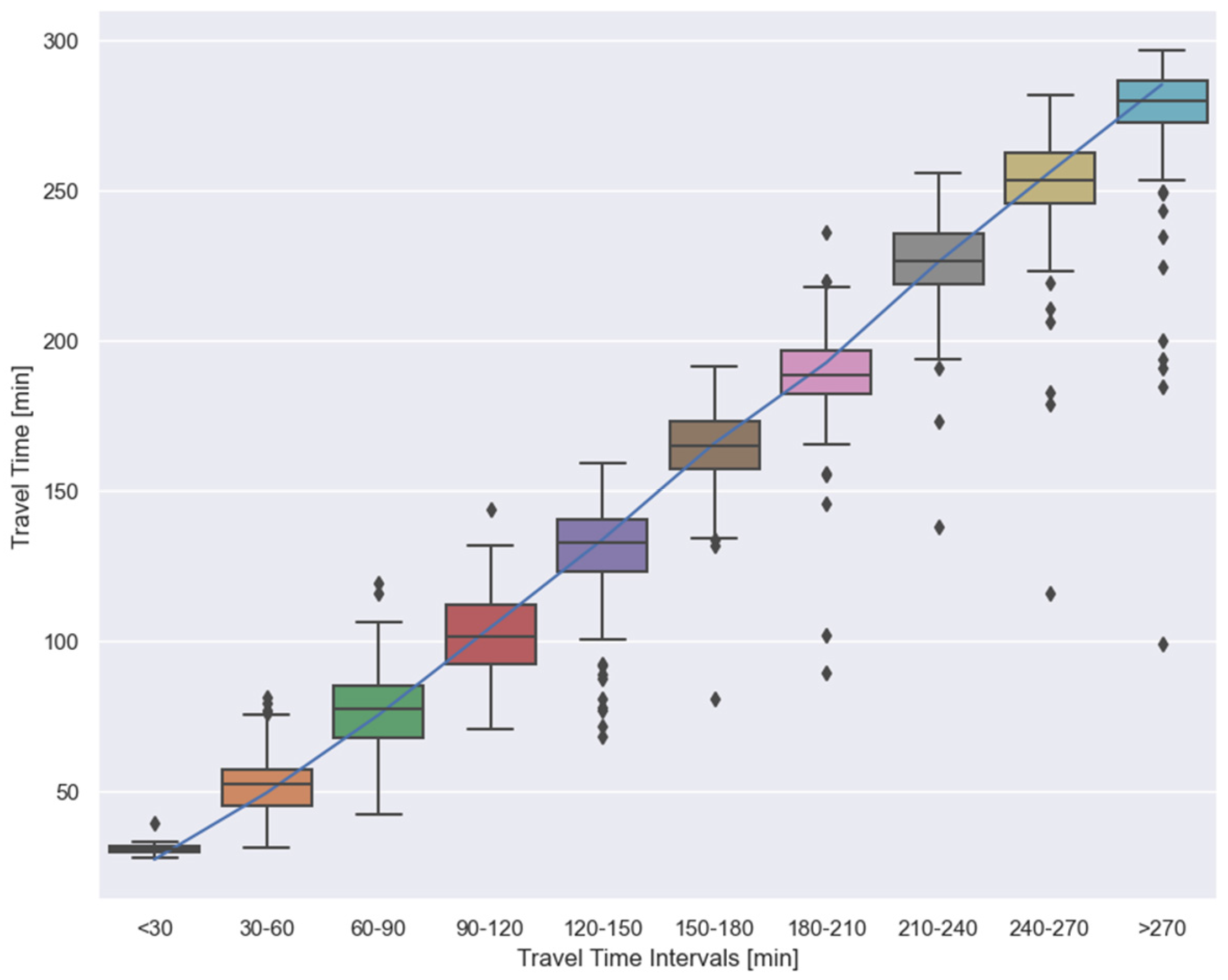
5.3. Apply Model
6. Conclusions
Author Contributions
Funding
Institutional Review Board Statement
Informed Consent Statement
Data Availability Statement
Conflicts of Interest
References
- Review of Maritime Transport; United Nations Publications: New York, NY, USA, 2022; ISBN 978-92-1-113073-7.
- Park, K.; Sim, S.; Bae, H. Vessel Estimated Time of Arrival Prediction System Based on a Path-Finding Algorithm. Marit. Transp. Res. 2021, 2, 100012. [Google Scholar] [CrossRef]
- Kang, M.J.; Hamidi, M. Quantifying and Predicting Waterway Traffic Conditions: A Case Study of Houston Ship Channel; Lamar University: Beaumont, TX, USA, 2021. [Google Scholar]
- Kabir, M.; Kang, M.J.; Wu, X.; Hamidi, M. Study on U-Turn Behavior of Vessels in Narrow Waterways Based on AIS Data. Ocean Eng. 2022, 246, 110608. [Google Scholar] [CrossRef]
- Cho, Y.; Park, J.; Kim, J.; Kim, J. Autonomous Ship Collision Avoidance in Restricted Waterways Considering Maritime Navigation Rules. IEEE J. Ocean. Eng. 2023, 48, 1009–1018. [Google Scholar] [CrossRef]
- Agafonov, A.; Yumaganov, A. Bus Arrival Time Prediction with LSTM Neural Network. In Proceedings of the Advances in Neural Networks—ISNN 2019; Lu, H., Tang, H., Wang, Z., Eds.; Springer International Publishing: Cham, Switzerland, 2019; pp. 11–18. [Google Scholar]
- Derrow-Pinion, A.; She, J.; Wong, D.; Lange, O.; Hester, T.; Perez, L.; Nunkesser, M.; Lee, S.; Guo, X.; Wiltshire, B.; et al. ETA Prediction with Graph Neural Networks in Google Maps. In Proceedings of the 30th ACM International Conference on Information & Knowledge Management, Gold Coast, QLD, Australia, 1–5 November 2021; Association for Computing Machinery: New York, NY, USA, 2021; pp. 3767–3776. [Google Scholar]
- Carr, G.C.; Erzberger, H.; Neuman, F. Fast-Time Study of Airline-Influenced Arrival Sequencing and Scheduling. J. Guid. Control Dyn. 2000, 23, 526–531. [Google Scholar] [CrossRef]
- Roy, K.; Levy, B.; Tomlin, C. Target Tracking and Estimated Time of Arrival (ETA) Prediction for Arrival Aircraft. In Proceedings of the AIAA Guidance, Navigation, and Control Conference and Exhibit; Guidance, Navigation, and Control and Co-located Conferences, Keystone, CO, USA, 21–24 August 2006; American Institute of Aeronautics and Astronautics: Reston, VA, USA, 2012. [Google Scholar]
- Lim, A.; Rodrigues, B.; Zhu, Y. Airport Gate Scheduling with Time Windows. Artif. Intell. Rev. 2005, 24, 5–31. [Google Scholar] [CrossRef]
- Narciso, M.E.; Piera, M.A. Robust Gate Assignment Procedures from an Airport Management Perspective. Omega 2015, 50, 82–95. [Google Scholar] [CrossRef]
- Yang, Z.; Wang, Y.; Li, J.; Liu, L.; Ma, J.; Zhong, Y. Airport Arrival Flow Prediction considering Meteorological Factors Based on Deep-Learning Methods. Complexity 2020, 2020, 6309272. [Google Scholar] [CrossRef]
- Ayhan, S.; Costas, P.; Samet, H. Predicting Estimated Time of Arrival for Commercial Flights. In Proceedings of the 24th ACM SIGKDD International Conference on Knowledge Discovery & Data Mining, London, UK, 19–23 August 2018; Association for Computing Machinery: New York, NY, USA; pp. 33–42. [Google Scholar]
- Karbassi, A.; Barth, M. Vehicle Route Prediction and Time of Arrival Estimation Techniques for Improved Transportation System Management. In Proceedings of the IEEE IV2003 Intelligent Vehicles Symposium. Proceedings (Cat. No.03TH8683), Columbus, OH, USA, 9–11 June 2003; pp. 511–516. [Google Scholar]
- Mazloumi, E.; Rose, G.; Currie, G.; Sarvi, M. An Integrated Framework to Predict Bus Travel Time and Its Variability Using Traffic Flow Data. J. Intell. Transp. Syst. 2011, 15, 75–90. [Google Scholar] [CrossRef]
- Achar, A.; Bharathi, D.; Kumar, B.A.; Vanajakshi, L. Bus Arrival Time Prediction: A Spatial Kalman Filter Approach. IEEE Trans. Intell. Transp. Syst. 2020, 21, 1298–1307. [Google Scholar] [CrossRef]
- Propp, D.A.; Rosenberg, C.A. A Comparison of Prehospital Estimated Time of Arrival and Actual Time of Arrival to an Emergency Department. Am. J. Emerg. Med. 1991, 9, 301–303. [Google Scholar] [CrossRef]
- Fleischman, R.J.; Lundquist, M.; Jui, J.; Newgard, C.D.; Warden, C. Predicting Ambulance Time of Arrival to the Emergency Department Using Global Positioning System and Google Maps. Prehospital Emerg. Care 2013, 17, 458–465. [Google Scholar] [CrossRef]
- Shmueli, G.; Bruce, P.C.; Patel, N.R. Data Mining for Business Analytics: Concepts, Techniques, and Applications with XLMiner; Wiley: Hoboken, NJ, USA, 2016; ISBN 9781118729137. [Google Scholar]
- Pani, C.; Vanelslander, T.; Fancello, G.; Cannas, M. Prediction of Late/Early Arrivals in Container Terminals—A Qualitative Approach. Eur. J. Transp. Infrastruct. Res. 2015, 15, 536–550. [Google Scholar] [CrossRef]
- Hart, P.E.; Nilsson, N.J.; Raphael, B. A Formal Basis for the Heuristic Determination of Minimum Cost Paths. IEEE Trans. Syst. Sci. Cybern. 1968, 4, 100–107. [Google Scholar] [CrossRef]
- Shin, Y.W.; Abebe, M.; Noh, Y.; Lee, S.; Lee, I.; Kim, D.; Bae, J.; Kim, K.C. Near-Optimal Weather Routing by Using Improved A* Algorithm. Appl. Sci. 2020, 10, 6010. [Google Scholar] [CrossRef]
- Alessandrini, A.; Mazzarella, F.; Vespe, M. Estimated Time of Arrival Using Historical Vessel Tracking Data. IEEE Trans. Intell. Transp. Syst. 2018, 20, 7–15. [Google Scholar] [CrossRef]
- Chen, X.; Wang, M.; Ling, J.; Wu, H.; Wu, B.; Li, C. Ship Imaging Trajectory Extraction Via an Aggregated you only Look once (YOLO) Model. Eng. Appl. Artif. Intell. 2024, 130, 107742. [Google Scholar] [CrossRef]
- Wu, X.; Roy, U.; Hamidi, M.; Craig, B.N. Estimate Travel Time of Ships in Narrow Channel Based on AIS Data. Ocean Eng. 2020, 202, 106790. [Google Scholar] [CrossRef]
- Wu, X.; Mehta, A.L.; Zaloom, V.A.; Craig, B.N. Analysis of Waterway Transportation in Southeast Texas Waterway Based on AIS Data. Ocean Eng. 2016, 121, 196–209. [Google Scholar] [CrossRef]
- Wu, X.; Rahman, A.; Zaloom, V.A. Study of Travel Behavior of Vessels in Narrow Waterways Using AIS Data—A CASE study in Sabine-Neches Waterways. Ocean Eng. 2018, 147, 399–413. [Google Scholar] [CrossRef]
- Roy, U.; Wu, X. Ais-data based vessel traffic’s characteristics and travel behaviour analysis: A case study at houston ship channel. J. Ocean Technol. 2019, 14, 58–74. [Google Scholar]
- Kang, L.; Meng, Q.; Liu, Q. Fundamental Diagram of Ship Traffic in the Singapore Strait. Ocean Eng. 2018, 147, 340–354. [Google Scholar] [CrossRef]
- Ghanim, M.S.; Shaaban, K.; Miqdad, M. An Artificial Intelligence Approach to Estimate Travel Time along Public Transportation Bus Lines. In Proceedings of the International Conference on Civil Infrastructure and Construction, Doha, Qatar, 2–5 February 2023. [Google Scholar]
- Liu, H.; Xu, H.; Yan, Y.; Cai, Z.; Sun, T.; Li, W. Bus Arrival Time Prediction Based on LSTM and Spatial-Temporal Feature Vector. IEEE Access 2020, 8, 11917–11929. [Google Scholar] [CrossRef]
- Petersen, N.C.; Rodrigues, F.; Pereira, F.C. Multi-Output Bus Travel Time Prediction with Convolutional LSTM Neural Network. Expert Syst. Appl. 2019, 120, 426–435. [Google Scholar] [CrossRef]
- Ranjitkar, P.; Tey, L.-S.; Chakravorty, E.; Hurley, K.L. Bus Arrival Time Modeling Based on Auckland Data. Transp. Res. Rec. J. Transp. Res. Board 2019, 2673, 1–9. [Google Scholar] [CrossRef]
- Larsen, G.H.; Yoshioka, L.R.; Marte, C.L. Bus Travel Times Prediction Based on Real-Time Traffic Data Forecast Using Artificial Neural Networks. In Proceedings of the 2020 International Conference on Electrical, Communication, and Computer Engineering (ICECCE), Istanbul, Turkey, 12–13 June 2020; pp. 1–6. [Google Scholar]
- Alam, O.; Kush, A.; Emami, A.; Pouladzadeh, P. Predicting Irregularities in Arrival Times for Transit Buses with Recurrent Neural Networks Using GPS Coordinates and Weather Data. J. Ambient. Intell. Humaniz. Comput. 2020, 12, 7813–7826. [Google Scholar] [CrossRef]
- Chondrodima, E.; Georgiou, H.; Pelekis, N.; Theodoridis, Y. Particle Swarm Optimization and RBF Neural Networks for Public Transport Arrival Time Prediction Using GTFS Data. Int. J. Inf. Manag. Data Insights 2022, 2, 100086. [Google Scholar] [CrossRef]
- Milenković, M.; Milosavljevic, N.; Bojović, N.; Val, S. Container Flow Forecasting through Neural Networks Based on Metaheuristics. Oper. Res. 2021, 21, 965–997. [Google Scholar] [CrossRef]
- Kourounioti, I.; Polydoropoulou, A.; Tsiklidis, C. Development of Models Predicting Dwell Time of Import Containers in Port Container Terminals—An Artificial Neural Networks Application. Transp. Res. Procedia 2016, 14, 243–252. [Google Scholar] [CrossRef]
- Gao, M.; Shi, G.; Li, S. Online Prediction of Ship Behavior with Automatic Identification System Sensor Data Using Bidirectional Long Short-Term Memory Recurrent Neural Network. Sensors 2018, 18, 4211. [Google Scholar] [CrossRef]
- Kim, J.; Lee, C.; Chung, D.; Kim, J. Navigable Area Detection and Perception-Guided Model Predictive Control for Autonomous Navigation in Narrow Waterways. IEEE Robot. Autom. Lett. 2023, 8, 5456–5463. [Google Scholar] [CrossRef]
- Fancello, G.; Pani, C.; Pisano, M.; Serra, P.; Zuddas, P.; Fadda, P. Prediction of Arrival Times and Human Resources Allocation for Container Terminal. Marit. Econ. Logist. 2011, 13, 142–173. [Google Scholar] [CrossRef]
- Pani, C.; Cannas, M.; Fadda, P.; Fancello, G.; Frigau, L.; Mola, F. Delay Prediction in Container Terminals: A Comparison of Machine Learning Methods. In Proceedings of the WCTR (World Conference on Transport Research), Rio de Janeiro, Brazil, 15–18 July 2013. [Google Scholar]
- Pani, C.; Fadda, P.; Fancello, G.; Frigau, L.; Mola, F. A data mining approach to forecast late arrivals in a transhipment container terminal. Transport 2014, 29, 175–184. [Google Scholar] [CrossRef]
- Pallotta, G.; Vespe, M.; Bryan, K. Vessel Pattern Knowledge Discovery from AIS Data: A Framework for Anomaly Detection and Route Prediction. Entropy 2013, 15, 2218–2245. [Google Scholar] [CrossRef]
- Parolas, I.; Tavasszy, L.; Kourounioti, I.; van Duin, R.; Cities, K. Prediction of Vessels’ Estimated Time of Arrival (ETA) Using Machine Learning–a Port of Rotterdam Case Study. In Proceedings of the 96th Annual Meeting of the Transportation Research, Washington, DC, USA, 8–12 January 2017; pp. 8–12. [Google Scholar]
- Noman, A.A.; Heuermann, A.; Wiesner, S.A.; Thoben, K.-D. Towards Data-Driven GRU based ETA Prediction Approach for Vessels on both Inland Natural and Artificial Waterways. In Proceedings of the 2021 IEEE International Intelligent Transportation Systems Conference (ITSC), Indianapolis, IN, USA, 19–22 September 2021; pp. 2286–2291. [Google Scholar]
- Yu, J.; Tang, G.; Song, X.; Yu, X.; Qi, Y.; Li, D.; Zhang, Y. Ship Arrival Prediction and Its Value on Daily Container Terminal Operation. Ocean Eng. 2018, 157, 73–86. [Google Scholar] [CrossRef]
- Notteboom, T.E. The Time Factor in Liner Shipping Services. Marit. Econ. Logist. 2006, 8, 19–39. [Google Scholar] [CrossRef]
- Available online: https://marinecadastre.gov/ (accessed on 1 January 2024).
- Sedaghat, A.; Kang, M.J.; Hamidi, M. A Heuristic ETL Process to Dynamically Separate and Compress AIS Data. In Proceedings of the 2023 Systems and Information Engineering Design Symposium (SIEDS), Charlottesville, VA, USA, 27–28 April 2023; pp. 159–164. [Google Scholar]
- Sedaghat, A.; Arbabkhah, H.; Kang, M.J.; Hamidi, M. Deep Learning Applications in Vessel Dead Reckoning to Deal with Missing Automatic Identification System Data. J. Mar. Sci. Eng. 2024, 12, 152. [Google Scholar] [CrossRef]
- Wold, S.; Esbensen, K.; Geladi, P. Principal component analysis. Chemom. Intell. Lab. Syst. 1987, 2, 37–52. [Google Scholar] [CrossRef]
- Chen, T.; Guestrin, C. XGBoost: A Scalable Tree Boosting System. In Proceedings of the 22nd ACM SIGKDD International Conference on Knowledge Discovery and Data Mining, San Francisco, CA, USA, 13–17 August 2016; Association for Computing Machinery: New York, NY, USA; pp. 785–794. [Google Scholar]


| Static Information | Dynamic Information |
|---|---|
| MMSI Number | Ship’s Position with Accuracy indication |
| IMO Number | Position timestamp (in UTC) |
| Name and Call Sign | Course Over Ground (COG) |
| Length and Beam | |
| Type of Ship | |
| Location of Position |
| Variable | Description |
|---|---|
| Data | AIS data of 4330 Cargo and Tankers |
| Historical Period | January 2018 to April 2020 |
| Features | MMSI, Vessel type, Date, Latitude, Longitude |
| Features | ||
|---|---|---|
| MMSI | Vessel Type | Trip Number |
| Direction | Date | Location |
| Segment id | ||
| Hyperparameter | Range | Increment Method | Optimal Value |
|---|---|---|---|
| (1 × 10⁻³, 10) | Loguniform | 0.009 | |
| (1 × 10−3,10) | Loguniform | 1.03 | |
| Colsample by tree | (0.3, 1.0) | 0.1 | 0.7 |
| Sub sample | (0.4, 1.0) | 0.1 | 0.4 |
| Learning rate | (0.008, 0.02) | 0.001 | 0.014 |
| Max depth | (10, 80) | 10 | 40 |
| Min child weight | (1, 300) | uniform | 5 |
| Metric | Tuned Full Model | Reduced Model |
|---|---|---|
| 0.99 | 0.98 | |
| 6.35 | 6.81 | |
| 95.01 | 105.21 | |
| 0.05 | 0.05 |
| Metric | Tuned Full Model | Reduced Model |
|---|---|---|
| 0.98 | 0.98 | |
| 6.49 | 6.41 | |
| 136.01 | 127.61 | |
| 0.05 | 0.05 |
Disclaimer/Publisher’s Note: The statements, opinions and data contained in all publications are solely those of the individual author(s) and contributor(s) and not of MDPI and/or the editor(s). MDPI and/or the editor(s) disclaim responsibility for any injury to people or property resulting from any ideas, methods, instructions or products referred to in the content. |
© 2024 by the authors. Licensee MDPI, Basel, Switzerland. This article is an open access article distributed under the terms and conditions of the Creative Commons Attribution (CC BY) license (https://creativecommons.org/licenses/by/4.0/).
Share and Cite
Arbabkhah, H.; Sedaghat, A.; Jafari Kang, M.; Hamidi, M. Automatic Identification System-Based Prediction of Tanker and Cargo Estimated Time of Arrival in Narrow Waterways. J. Mar. Sci. Eng. 2024, 12, 215. https://doi.org/10.3390/jmse12020215
Arbabkhah H, Sedaghat A, Jafari Kang M, Hamidi M. Automatic Identification System-Based Prediction of Tanker and Cargo Estimated Time of Arrival in Narrow Waterways. Journal of Marine Science and Engineering. 2024; 12(2):215. https://doi.org/10.3390/jmse12020215
Chicago/Turabian StyleArbabkhah, Homayoon, Atefe Sedaghat, Masood Jafari Kang, and Maryam Hamidi. 2024. "Automatic Identification System-Based Prediction of Tanker and Cargo Estimated Time of Arrival in Narrow Waterways" Journal of Marine Science and Engineering 12, no. 2: 215. https://doi.org/10.3390/jmse12020215
APA StyleArbabkhah, H., Sedaghat, A., Jafari Kang, M., & Hamidi, M. (2024). Automatic Identification System-Based Prediction of Tanker and Cargo Estimated Time of Arrival in Narrow Waterways. Journal of Marine Science and Engineering, 12(2), 215. https://doi.org/10.3390/jmse12020215