Enhancing Wave Energy Conversion Efficiency through Supervised Regression Machine Learning Models

Abstract

The incorporation of machine learning (ML) has yielded substantial benefits in detecting nonlinear patterns across a wide range of applications, including offshore engineering. Existing ML works, specifically supervised regression models, have not undergone exhaustive scrutiny, and there are no potential or concurrent models for improving the performance of wave energy converter (WEC) devices. This study employs supervised regression ML models, including multi-layer perceptron, support vector regression, and XGBoost, to optimize the geometric aspects of an asymmetric WEC inspired by Salter’s duck, based on key parameters. These important parameters, the ballast weight and its position, vary along a guided line within the available geometric resilience of the asymmetric WEC. Each supervised regression ML model was fine-tuned through hyperparameter optimization using Grid cross-validation. When evaluating the performance of each ML model, it became evident that the tuned hyperparameters of XGBoost led to predictions that strongly aligned with the actual values compared to other models. Furthermore, the study extended to assess the performance of the optimized WEC at the designated deployment test site location.

1. Introduction

In the current global context, the issue of global warming has taken on monumental proportions, prompting nations worldwide to actively seek out environmentally friendly alternatives to traditional fossil fuels [1,2,3]. This contemporary era witnesses a heightened urgency to address this crisis, far surpassing the urgency of earlier times. The exploration of alternative renewable energy sources has gained substantial momentum, with a notable focus on solar, wind, and ocean wave energy [4,5,6]. While solar and wind power have successfully advanced to a level of mature commercialization, the potential of ocean wave energy remains a compelling avenue to pursue. Despite its promise, the extraction of energy from waves continues to face various challenges. These hurdles encompass issues such as efficiency limitations and the high deployment costs associated with wave energy technologies [7,8,9]. Consequently, the commercial landscape lacks fully realized wave energy structures at present [10,11]. Nevertheless, a multitude of researchers hold the view that ocean wave energy represents an immensely promising sector for the development of sustainable, green energy solutions. This sentiment underscores the potential inherent in this field and encourages further exploration into unlocking its viability for widespread adoption [7,12,13].

Within the realm of ocean wave energy systems, a few researchers [14,15,16] have attempted to analyze the sustainability, reliability, and economic feasibility of real sea conditions for small islands. Nezhad et al. [14] employed numerical simulations and data analysis to find the performance metrics of different wave energy converter technologies (WEC), such as Wave Star, Oyster, Wave Dragon and Archimedes Wave Swing. Based on the capacity factor, rated capacity factor, and operation time, a best WEC has been selected among the alternatives. 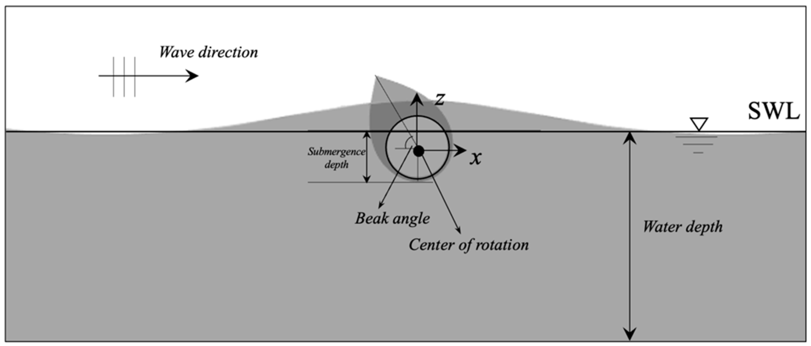But in 1975 and 1976, Salter [17,18] claimed that a nodding duck WEC was recorded as being a particularly efficient device within ocean wave energy systems, especially in the context of 2D regular wave conditions known as Salter’s duck (asymmetric WEC), which is a pitch-type device. Examining Figure 1, the arrival of the foreside of the WEC is grounded in the displacement of fluid particles, while the leeside is formed by a circular pattern, resulting in an asymmetric WEC shape. The basic concept of the asymmetric WEC centers on its ability to pitch in harmony with pressure-induced motions around the central axis of rotation. Along with the dynamic pressure, the variation in hydrostatic pressure further contributes to the rotation by causing the buoyant foreside near the beak to oscillate (as illustrated in Figure 1). This distinctive characteristic enhances overall performance, allowing for the successful conversion of both kinetic and potential energies generated by the waves into rotational mechanical energy. The evolutionary trajectory of the asymmetric WEC has witnessed the integration of experimental approaches [19,20,21] and numerical methods [22,23,24] to enhance its performance across a spectrum of sea states. Notably, the efficiency of this technology experiences a substantial decline when confronted with the intricate variations in incoming waves, encompassing factors such as high steep waves, 3D nonlinear effects, and the influence of waves breaking in the proximity of the WEC. These dynamic wave conditions can lead to a notable reduction in efficiency. In response to these challenges, numerous researchers have used nonlinear models to investigate the complex behavior of the asymmetric WEC, uncovering factors that contribute to its suboptimal performance [22,25]. To surmount these limitations, innovative strategies have been explored, including the incorporation of mechanisms such as negative stiffness, which have shown promising results in augmenting the device’s efficiency [26,27]. Studies have demonstrated that the introduction of negative stiffness mechanisms in both linear and nonlinear wave scenarios can lead to significant improvements in efficiency. However, it is important to acknowledge that existing models of asymmetric WECs have not undergone exhaustive scrutiny in terms of fundamental geometric design optimization, leading to performance fluctuations in varying wave environments. Recognizing this critical gap, recent research efforts have turned to machine learning (ML) to tackle the challenge of optimizing the performance of WECs [28,29,30]. By harnessing the power of machine learning strategies, researchers aim to enhance the predictability and adaptability of WECs, thereby paving the way for more consistent and efficient energy generation from ocean waves.

Machine learning methods offer a pivotal advantage in their capacity to identify and comprehend nonlinear patterns present within provided input data, enabling them to provide accurate approximations and adapt swiftly to evolving environments. This adaptability is especially pertinent given the inherent challenge of optimizing the performance of designed WECs in the face of constantly shifting environmental conditions [31]. Li et al. [32] harnessed the power of artificial neural networks (ANNs), employing real-time latching control to enhance the performance of a heaving point absorber in irregular waves. Their ANNs, built upon the backpropagation algorithm, demonstrated an impressive outcome—by manipulating the velocity phase through real-time control, they achieved energy extraction rates as high as 80%, a marked improvement facilitated by the intelligent controller. Building on this foundation, Li et al. [33] extended their research to address prediction deviations in this context. Liu et al. [34] conducted a comprehensive exploration employing smooth particle hydrodynamics to optimize surge-type WECs through distinct geometric design parameters. Leveraging a dataset comprising 379 input parameters—encompassing wave periods, wave heights, and water depths—they utilized an ANN model based on radial basis function neural networks. Their findings were significant, showcasing the versatility of the ANN model in not only optimizing WEC design but also tackling intricate technical optimization challenges. George et al. [35] adopted the potential of ANNs to maximize energy extraction from U-shaped oscillating water column (OWC) devices aided by a bottom-attached plate. By generating input data through a random assortment of 4000 cases—manipulating barrier height, interbarrier distance, and chamber wall submergence depth through analytical modeling—they trained their ANN model with 70% of this dataset and validated its performance using the remaining data. This approach yielded remarkable results, with the trained ANN model exhibiting a high R-squared (R²) score of 0.95, underscoring its efficacy. Poguluri et al. [30] took an innovative approach by employing an ANN-based multi-layer perceptron (MLP) regression model to optimize the design of asymmetric WECs. Demonstrating their technique’s potential, they achieved an 11% increase in extracted power compared to the original WEC model under design wave conditions, showcasing the practicality and benefits of their MLP regression algorithm.

The studies mentioned earlier emphasize the increasing importance of incorporating ML techniques to overcome the complex challenges associated with optimizing WECs and advancing ocean wave energy extraction. The focus of the present investigation centers around optimizing key design parameters, particularly within the context of the asymmetric WEC. Of significant importance are the ballast weight and its position, as these elements profoundly influence the natural frequency of the WEC. Altering both the position and weight of the ballast induces changes in the internal moment of inertia and overall weight, consequently leading to variations in the WEC’s response. This dynamic adjustment proves pivotal for achieving efficient operation and enhancing the performance of these specific WECs. The primary objective is to optimize the hyperparameters of these ML models while examining their impact on performance using the framework of the linear potential flow theory. The study involves analyzing 25 distinct asymmetric WEC configurations, with a detailed investigation of each design. The focus of the present investigation is the optimization of key design parameters, specifically the position and location of the ballast weight, which are crucial for the efficient operation of these WECs. Overall, previous research has laid a foundation by showcasing the potential of ML in WEC optimization. This present study takes an innovative approach by focusing on fine-tuning hyperparameters within various supervised regression ML models and their application to the asymmetric WEC, addressing a critical knowledge gap and contributing to the overarching endeavor of harnessing ocean wave energy more effectively.

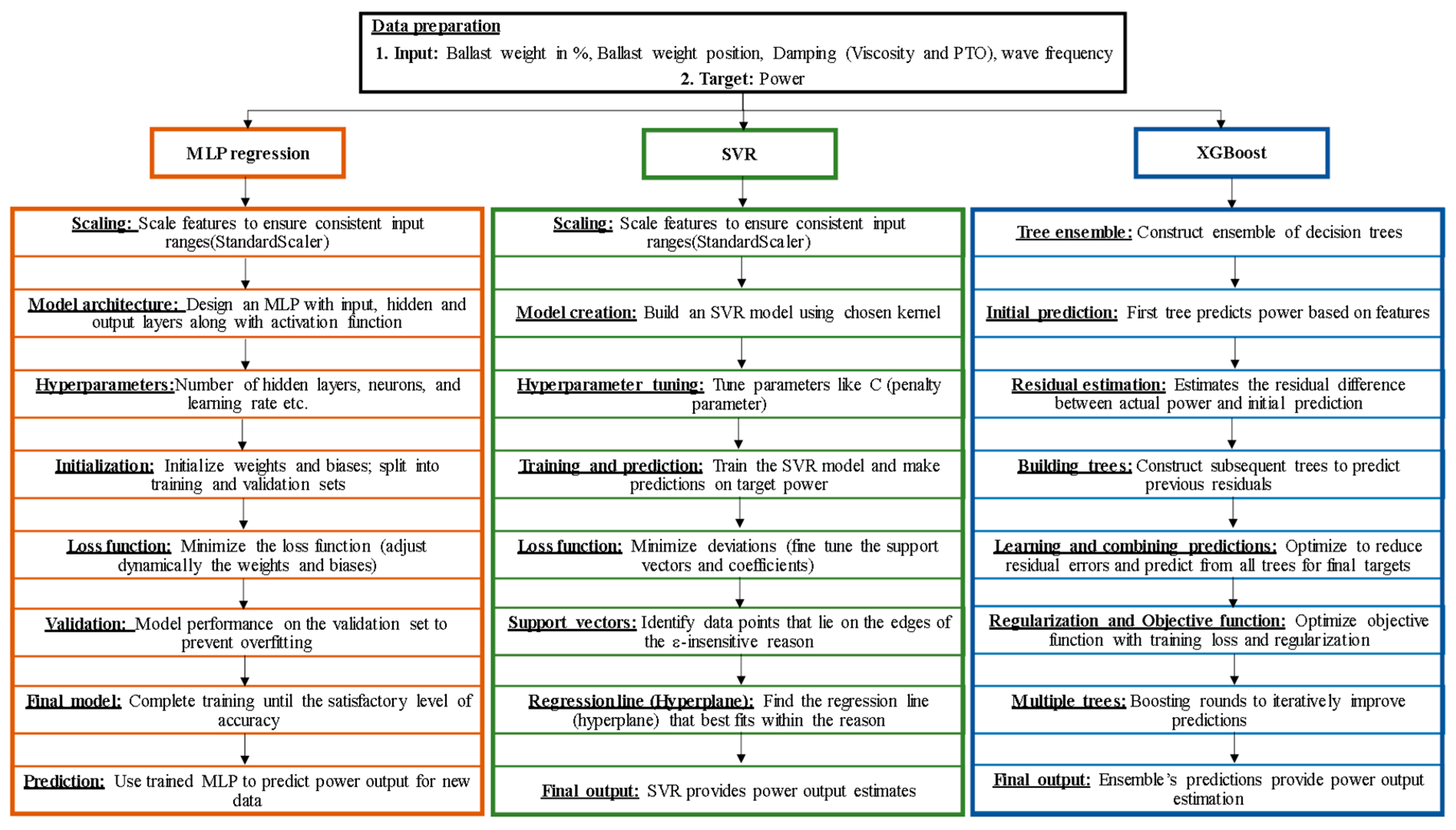
2. Supervised Machine Learning Models

ML models excel at identifying patterns within input data, even when presented randomly, and they adapt quickly to changing environments. Utilizing supervised learning among the ML models is advantageous, as these models comprehend the relationship, influence, and underlying patterns between input and target variables on a training set. The present study explores the supervised regression learning models (MLP, support vector regression and XGBoost) in optimizing the initial design of the asymmetric WEC. In this current study, Python 3.0 programming serves as the key tool for harnessing the potential of the supervised learning module offered by scikit-learn. The primary goal is to take full advantage of the diverse functionalities available in the open literature, optimizing and refining the application of these models specifically for investigating asymmetric WEC. By leveraging scikit-learn’s extensive capabilities, the coding implementation aims to enhance the efficiency and adaptability of these supervised learning models within the context of WEC analysis. This approach not only facilitates a more nuanced exploration of the complex dynamics associated with wave energy but also ensures a tailored and optimized utilization of machine learning techniques for the specific requirements of the study. The following methodology has been applied at various stages of the investigation and is summarized as detailed below.

• Data Preparation Stage #1:

In this initial stage, the dataset is prepared by considering 25 different WEC configurations. These configurations are achieved by systematically varying the ballast weight and its location, and the corresponding responses and power are obtained using Equations (4) and (7). The configurations are then exposed to a range of wave frequencies, resulting in a comprehensive input dataset consisting of 2850 data points.

• Training and Testing Stage #2:

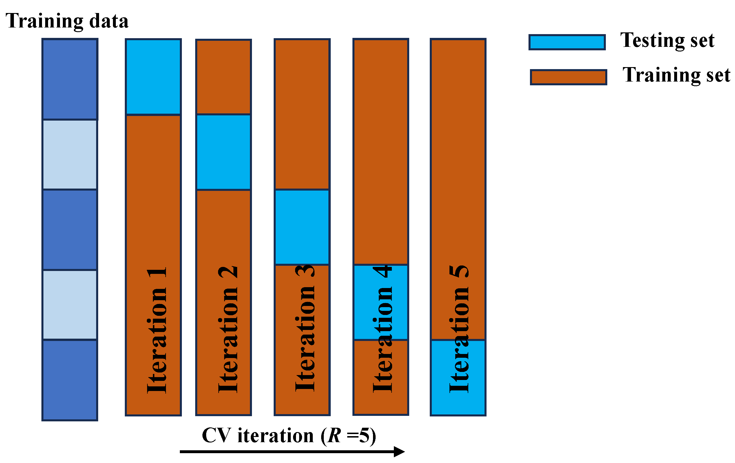
The generated input dataset is utilized for training and testing the supervised ML models. The process involves employing GridSearchCV in conjunction with five-fold cross-validation. This means that, for each set of hyperparameters associated with each supervised ML model, the training and evaluation processes are repeated five times. During each iteration, a distinct fold is designated for testing, while the remaining folds are used for training. The use of cross-validation enhances the robustness of the model evaluation, providing a more reliable assessment of each model’s performance.

The performance of each ML model is assessed against the input dataset, and a model with superior predictive capabilities is selected for further optimization.

• Optimization Stage #3:

In the optimization stage, a new dataset is generated, comprising 10,000 distinct WEC configurations. These configurations are created using a LHS model, which ensures a systematic and diverse selection of input parameters. The predetermined values of the input parameters are utilized to generate this expanded dataset. This newly created dataset serves as the basis for further optimization. The optimization stage aims to identify the optimum WEC configuration based on the trained ML model predictions.

2.1. Multi-Layer Perception Model

Within the context of pattern recognition, the MLP regression emerges as one of the most successful supervised models. This success can be attributed to its unique characteristics, where the number of basis functions (represented as ϕ_j(x)) corresponding to input variables is predetermined, yet the adaptability to fine tune these functions during the training phase is retained. This model, often referred to as a feed-forward neural network, operates by transmitting data unidirectionally from the input variables through to the target variables (Figure 2). Despite its intricate architecture, which encompasses multiple layers of logistic regression with continuous nonlinearities, the MLP model remains remarkably streamlined in practical application, leading to swifter computational processes. This study embarks on an expedition to assess and scrutinize the viability of implementing the MLP model in the context of the asymmetric WEC (Figure 2). The primary objectives of this evaluation revolve around the compactness of the model and its efficiency in computation. The core of the MLP model lies in its intricate web of interconnected neurons, each facilitating the exchange of information with its peers. Central to this information flow are the weights (denoted as w_j) assigned to the connections interlinking the various layers. The process of training the MLP model involves the dynamic adjustment of these weights in conjunction with the input variables, ultimately leading to a refined model capable of capturing intricate relationships within the data. The fundamental neural network model employs basis functions alongside a sigmoidal output unit activation function, which is expressed as [31,36]:

$$y_k\left(x,w\right) = \sigma \left({\displaystyle \sum _{j=1}^M{w}_{kj}^2{z}_j+w_{k0}^2}\right)\mathrm{where}{z}_j= h\left({\displaystyle \sum _{i=1}^D{w}_{ji}^{(1)}{x}_i+x_{j0}^{(1)}}\right)$$

(1)

w_jo, w_ko—bias parameters and j (1… M) has the linear combination of neutrons and (k = 1… K) is the total number of outputs. ‘h’ is the function of nonlinear activation function usually given by logistic sigmoid or tanh. The superscript represents the layer. x_i (i = 1… D) is the total number of input variables, y_k and both are controlled by vector.

2.2. Support Vector Regression

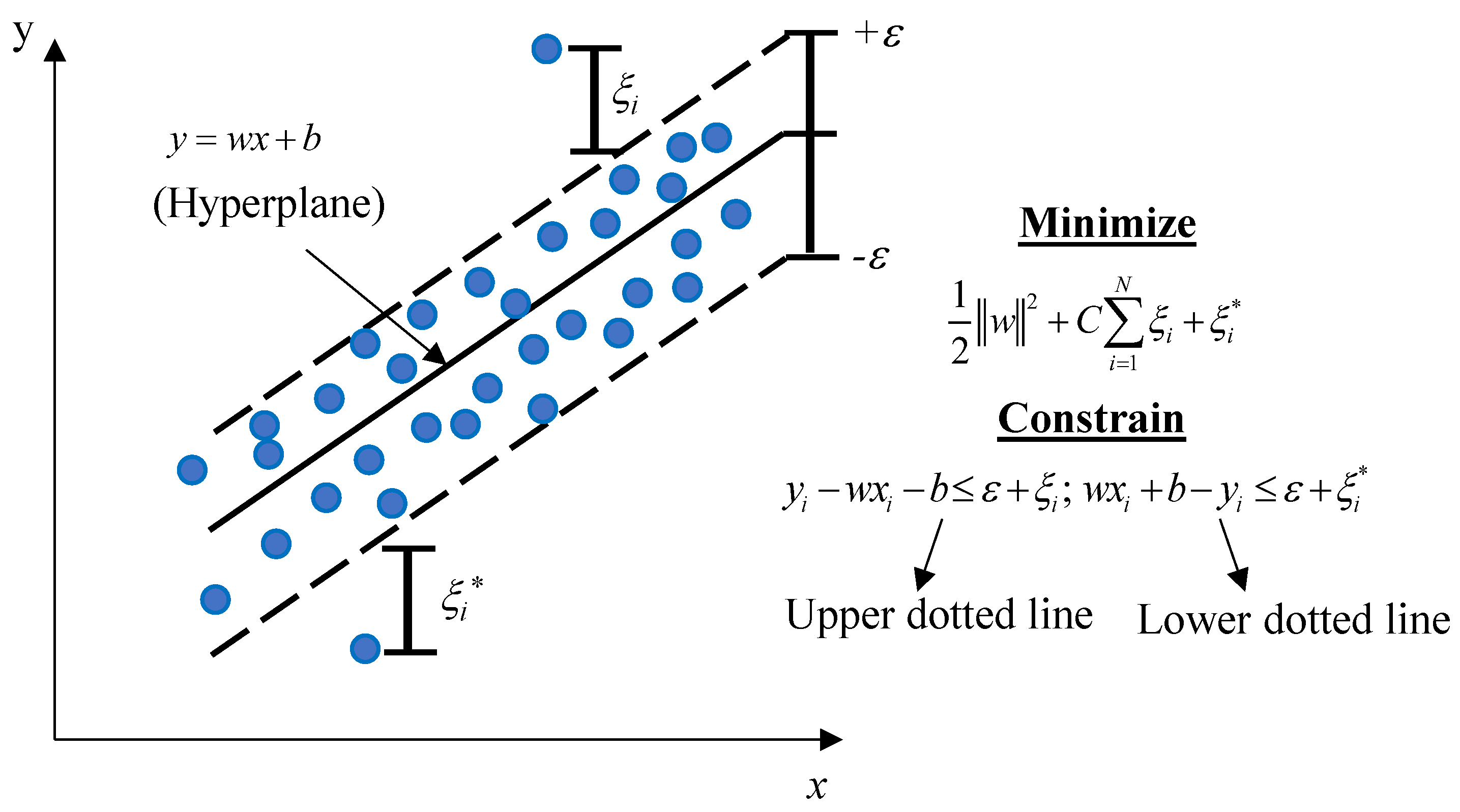
A support vector regression (SVR), which belongs to the broader category of support vector machines, is a sophisticated model employed in supervised learning scenarios. The essence of the SVR lies in its capacity to discern complex patterns within data. This is achieved through the fitting of a hyperplane, a multidimensional surface, that adeptly accommodates the largest attainable number of data points while adhering to a defined margin of tolerance, represented by the ε symbol (Figure 3). A visual representation of this concept can be found in Figure 3. Within the dataset that the SVR operates upon, there exist certain data points that fall outside the specified margin of tolerance. These points are referred to as slack variables, denoted as ξ_i and ξ_i*. They essentially signify the extent to which certain observations deviate from the idealized hyperplane. In order to refine the model’s accuracy, optimization techniques are employed. These techniques involve penalizing the aforementioned slack variables, effectively minimizing their impact on the overall model. The core objective of the optimization process is to maximize the margin, which in turn is tantamount to minimizing a carefully constructed monotonically decreasing function of weights. Accompanying this objective is a tuning parameter labeled as C. This parameter holds the dual role of being a hyperparameter and a key factor in the intricate balance between two vital components of the model: bias and variance (see Figure 3). The interplay of bias and variance significantly influences the model’s predictive capacity. In visualizing this interplay, the parameter C and its effect are also depicted in Figure 3. It is important to note that adjustments to the C parameter entail distinct outcomes. An augmentation of the C parameter results in a reduction of bias-a model’s tendency to oversimplify data at the cost of ignoring finer details. Conversely, this augmentation introduces a rise in variance-the model’s susceptibility to minor fluctuations within the training data. A decrease in the C parameter, on the other hand, tilts the balance toward higher bias and lower variance, potentially leading to an overly rigid model. Hence, the selection of the appropriate C value is a pivotal decision that encapsulates the model’s ability to find the optimal equilibrium between accuracy and generalizability.

2.3. XGBoost

XGBoost falls within the category of tree-based methods. These techniques offer numerous advantages, including high precision, user friendliness, and resilience to input scale variations. Furthermore, they exhibit impressive performance even with minimal tuning efforts see Chen et al. [37]. For a scenario with K trees, where the predictive outcome for each decision at the t-th step can be represented as:

$${\widehat{y}}_i^{(t)} = {\displaystyle \sum _{k=1}^t{f}_k\left(x_i\right)}$$

(2)

Here, f_k represents the prediction from an individual decision tree. The primary goal of the training process is to effectively optimize both the loss function (L) and the regularization term (Ω). This can be expressed as the objective function:

$$\mathrm{Objective}(Obj)=L+\Omega \mathrm{where}L = \frac{1}{N} {\displaystyle \sum _{i=1}^N{\left(y_i - {\widehat{y}}_i\right)}^2}\mathrm{and}\Omega = \gamma T+\frac{1}{2}\lambda {\displaystyle \sum _{j=1}^T{\left(w_j^2\right)}^2}$$

(3)

In this equation, T denotes the number of leaves, and $w_j^2$ signifies the score associated with the j-th leaf. The loss function governs the model’s predictive capacity, while the regularization term controls its simplicity, thereby preventing overfitting. To compute the gradient descent for optimizing the objective, an iterative technique is employed at each step, which is given by ${\partial }_{\widehat{y}}Obj\left(y,\widehat{y}\right)$. This technique adjusts the predicted outcome (denoted as $\widehat{y}$) along the gradient direction, aiming to minimize the overall objective. A prevailing challenge with these models is the tendency to encounter overfitting, which necessitates careful mitigation strategies. Expanding on this notion, proactive measures must be taken to avoid the detrimental effects of overfitting and ensure the model’s generalization capability.

3. Hyperparameter Optimization

As outlined in the preceding section, the core aim of a supervised regression ML model revolves around achieving optimal predictive performance when applied to new data. To effectively identify suitable values for intricate parameters within a model, it becomes imperative to thoroughly explore a range of hyperparameters and their potential combinations. This exploration is especially critical in the context of asymmetric WEC. While assessing the model’s performance on the training set holds importance, it may not consistently translate to accurate predictions for unseen data. To counteract the risk of overfitting, the inclusion of a distinct test set is recommended. Evaluating the chosen model’s performance benefits from the involvement of an independent validation set, comprising a substantial volume of data. This validation set, in conjunction with the training and testing sets, plays a pivotal role in pinpointing the model that offers the highest predictive proficiency. By allocating a fraction (R − 1)/R (R-fold) of the available data for training purposes while employing the entire dataset for performance assessment, the cross-validation (CV) strategy strikes a balance. To manage computational demands, it is essential to control the number of training runs, which tends to scale exponentially with R. The utilization of CV, visually depicted in Figure 4 with R = 5 and associated process. Efficiently navigating through various parameter configurations necessitates a strategy anchored solely in training data, impervious to overfitting biases. In the context of our specific problem, a set of supervised models has been cataloged, along with their corresponding hyperparameters and optimal combinations (as detailed in

Table 1. List of optimal hyperparameter combinations across various supervised regression ML models.

Supervised Models	Hyperparameters	Optimum Parameters
MLP Regression (Total number of fits 40320)	Number of layers:	Number of layers:
	(10, 10), (20, 10), (20, 20), (20, 30), (30, 30), (10, 10, 10), (20,20,20), (30, 30, 30)	(20, 20)
	Initial learning rate:	Initial learning rate:
	0.01, 0.005, 0.001	0.005
	Solver for weight optimization:	Solver for weight optimization:
	adam, lbfgs, sgd	adam
	Batch size:	Batch size:
	1, 20, 50, 100	20
	Alpha:	Alpha:
	10-1 to 101 with total of 7 values	0.316
	Activation function:	Activation function:
	identity, logistic, tanh, relu	Relu
SVR (Total number of fits 13440)	Kernel:	Kernel:
	linear, poly, rbf, sigmoid	rbf
	Degree:	Degree:
	2, 3, 4	3
	Gamma:	Gamma:
	Scale, auto with 10-3 to 102 with 6 values	1
	C:	C:
	10-3 to 103 with 7 values	1000
	Epsilon:	Epsilon:
	0.01, 0.1, 0.2, 0.5	0.1
XGBoost (Total number of fits 1500)	Gamma:	Gamma:
	0, 0.01, 0.1, 0.5, 1	0.01
	Learning:	Learning:
	0.01, 0.1, 0.2, 0.3	0.1
	Max. depth:	Max. depth:
	3, 4, 5, 6, 9	9
	n estimator:	n estimator:
	50, 100, 200	200
	Random state:	Random state:
	2021	2021

). This rigorous selection procedure aims to yield a robust and effective model configuration tailored to our asymmetric WEC application.

4. Data Preprocessing

In contrast to the prior approaches, the present study amalgamates sophisticated technical analysis with ML methodologies to extract nuanced insights into the optimal design of asymmetric WECs. By leveraging a broad spectrum of variables and scenarios, which strive to pave the way for highly efficient and adaptable WEC systems that can harness wave energy with unprecedented efficacy. The performance enhancement of asymmetric WECs hinges on a multitude of pivotal parameters that play a pivotal role. These parameters include the shape of the WEC, beak length, beak angle, depth of submergence, ballast weight distribution, and the damping aspects involving power take-off (PTO) mechanisms and viscosity effects. The illustration in Figure 5 provides an insightful depiction of the asymmetric WEC, highlighting its key parameters and its effect. In a study conducted by Poguluri et al. [38] utilizing a frequency domain solution, a systematic optimization of WEC parameters was undertaken. This optimization was tailored to align with the unique conditions around Jeju western island, encompassing both regular and irregular wave scenarios. Subsequent to these investigations, the scope was extended to encompass a computational fluid dynamics (CFD) analysis, thereby refining and expanding the understanding of asymmetric WECs. In this study, the foundational WEC design that stems from these investigations serves as the fundamental background for a novel approach. This approach involves the utilization of supervised regression ML models, as elaborated upon in Section 2, where the adopted final WEC is reminiscent of the work by Poguluri et al. [38]. This model-driven exploration for optimal design delves into various factors, notably the ballast weight associated with the asymmetric WEC and its spatial positioning, in conjunction with the externally influenced variables such as viscosity and PTO damping.

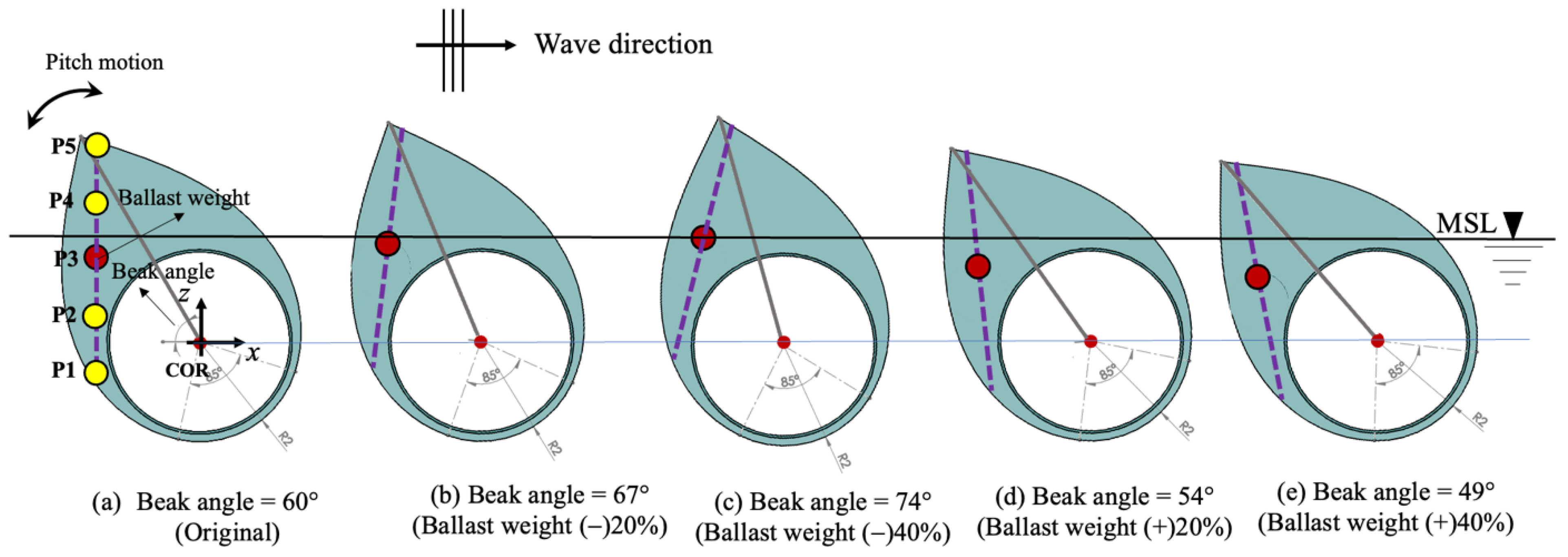
To examine the technical parameters, a 3D linear radiation–diffraction method is harnessed, coupled with potential flow theory, where the fluid flow is considered steady, incompressible, and inviscid. This approach relies on the widely recognized WAMIT framework, encapsulating the complexity of wave interactions with the WEC. The crux of the study lies in the design of 25 distinct WEC rotor configurations, featuring varying percentages of ballast weight: 0%, +20%, +40%, −20%, and −40%. With respect to the variation in ballast weight percentage, a weight of 0% signifies that no additional weight has been added, indicating the original weight remains unchanged. Conversely, when a ballast weight adjustment of +20% is mentioned, it indicates an increase of 20 percentage points from the original weight, as outlined in the second column of

Table 2. Total number of generated input data from 25 variants of designed asymmetric WECs.

S. No.	Ballast Weight	Ballast Position	Total Mass	Beak Angle	Center of Gravity (xg, zg)	Wave Frequency (ω)	Pitch Moment of Inertia About COR
Cases	[%]	[ m]	[kg]	[deg]	[m]	[rad/s]	[k·kg·m2]
0~569	0	P1 P2 P3 P4 P5	36,399.04	59	(−0.544, 0.952)	P1 <ω0… ω113> P2 <ω114… ω227> P3 <ω228… ω341> P4 <ω342… ω455> P5 <ω456… ω569>	205.88
				60	(−0.528, 0.774)		162.43
				60	(−0.528, 0.586)		133.24
				60	(−0.528, 0.399)		118.29
				60	(−0.528, 0.211)		117.59
570~1139	(−)20		35,080.13	114	(0.417, 0.887)	P1 <ω570… ω683> P2 <ω684… ω797> P3 <ω798… ω911> P4 <ω912… ω1025> P5 <ω1026… ω1139>	182.52
				69	(−0.357, 0.768)		147.82
				67	(−0.402, 0.601)		124.50
				65	(−0.436, 0.432)		112.56
				64	(−0.455, 0.269)		112.00
1140~1709	(−)40		33,761.22	98	(0.135, 0.843)	P1 <ω1140… ω1253> P2 <ω1254… ω1367> P3 <ω1368… ω1481> P4 <ω1482… ω1595> P5 <ω1596… ω1709>	159.16
				79	(−0.186, 0.727)		133.20
				74	(−0.278, 0.591)		115.76
				71	(−0.332, 0.457)		106.83
				69	(−0.366, 0.325)		106.41
1710~2279	(+)20		37,717.95	45	(−0.786, 0.914)	P1 <ω1710… ω1823> P2 <ω1824… ω1937> P3 <ω1938… ω2051> P4 <ω2052… ω2165> P5 <ω2166… ω2279>	229.23
				52	(−0.690, 0.751)		177.05
				54	(−0.641, 0.558)		141.98
				55	(−0.612, 0.3523)		124.03
				56	(−0.591, 0.146)		123.18
2280~2849	(+)40		39,036.85	41	(−0.966, 0.880)	P1 <ω2280… ω2393> P2 <ω2394… ω2507> P3 <ω2508… ω2621> P4 <ω2622… ω2735> P5 <ω2736… ωω2849>	252.59
				46	(−0.826, 0.723)		191.67
				49	(−0.746, 0.524)		150.72
				51	(−0.683, 0.307)		129.76
				53	(−0.642, 0.087)		128.78

and subsequent variations in ballast weight, following the same pattern. The positioning of these ballast weights is diversified across five distinct combinations, guided along with the reference points P1, P2, P3, P4, and P5, as shown in Figure 5. P3 designates the initial position, situated at the midpoint of the guided line. In contrast, P1, P2, and P4, P5 denote locations both above and below, evenly spaced along the guided line as indicated in Figure 5. Furthermore, Figure 5 illustrates the standard initial orientation of the asymmetric WEC rotor, depicting how it changes as the ballast weight percentage varies. This occurs while the rotor remains fixed at position P3. Consequently, these diverse configurations are subjected to a comprehensive array of wave frequencies spanning the range from 0.01 rad/s to 10 rad/s, with an incremental step of 0.01 rad/s. This exhaustive exploration yields a total of 2850 distinct scenarios, each serving as a valuable input for the adopted ML models.

The operational behavior of the asymmetric WEC revolves around a constrained pitch-type motion pivoting about its central rotation point. This movement is characterized by the interaction of a select set of pivotal forces, where the cumulative inertial forces are balanced by the reactive force system acting upon the WEC. These intricate total forces can be dissected into two primary categories: 1. hydrodynamic forces and hydrostatic forces and 2. external loads that collectively shape the dynamics of the system. The hydrodynamic forces encapsulate a range of elements, encompassing both excitation forces (Froude-Krylov and diffraction forces) and radiation forces. These forces, coupled with the hydrostatic restoring moment, manifest as pressures acting upon the asymmetric WEC. In a complementary manner, the reaction forces emanate from the PTO mechanism and the influence of viscosity. These forces further contribute to the holistic force equilibrium governing the behavior of the asymmetric WEC. Navigating through this intricate wave interactions yields an expression encapsulating the behavior of the WEC along the pitch mode. Expressed in complex amplitude, this comprehensive formulation captures the nuanced interplay of all contributing forces and moments, revealing the intricate dynamics of the asymmetric WEC’s pitch mode given by

$$\xi = F_E/\left(\left[-{\omega }^2(m+A) +K\right]+ i\omega (B_{rad} + B_{vis}+ B_{PTO}) \right)$$

(4)

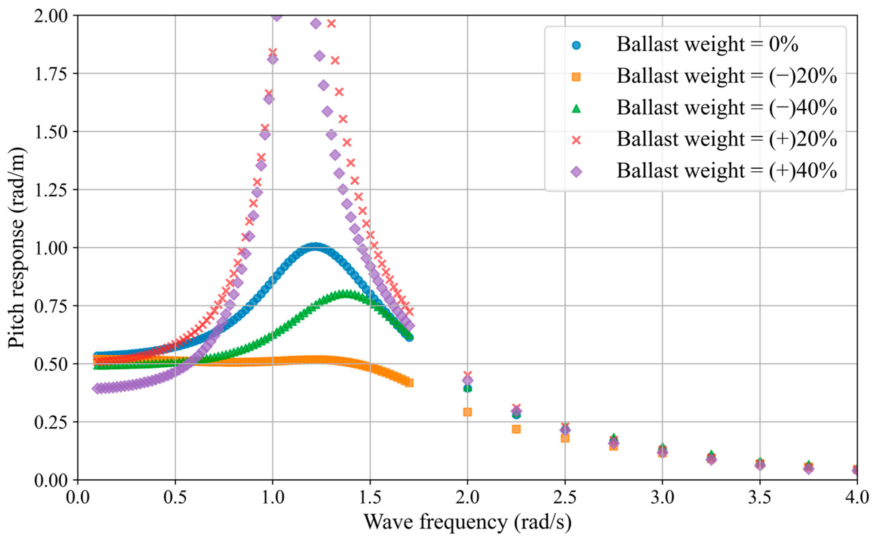
Commencing with the pitch response amplitude operator (RAO)—$\xi /a$, where ‘a’ signifies the wave amplitude, Figure 6 illustrates its variation across the designed WECs. The plot captures the changes in RAO as the wave frequency changes.

Utilizing the aforementioned equation, the nondimensional representation of the pitch response ($\xi /a$) is graphically presented for instances of the asymmetric WECs, typically for the P3 ballast position, as depicted in Figure 6. To ascertain the mean extracted power (P_avg), the following expression is invoked:

$$P_{avg}/a^2=\frac{1}{2}{\omega }^2{B}_{PTO}^{}{\left|\xi /a\right|}^2$$

(5)

where ‘ω’ denotes the wave frequency and ‘B_PTO’ is the parameter associated with the PTO mechanism. This equation encapsulates the essence of power extraction from the system, providing a metric for evaluating performance. The quest for optimal power extraction leads to the concept of the optimal PTO configuration (${\tilde{B}}_{PTO}^{}$) where the variation of B_PTO is depicted in Figure 7 only for the P3 ballast position of the WEC. In standard practice, the variable optimal PTO damping moment is frequently employed in the frequency domain solution to derive the optimal power output. However, for the sake of optimism, a fixed PTO damping moment is utilized, representing the minimum optimal PTO value obtained through Equation (6), as illustrated in Figure 7. This optimal PTO value is determined by setting the $\partial P_{avg}/\partial B_{PTO} = 0$ to achieve maximum power extraction, emphasizing a strategic approach to enhance power capture efficiency. Notably, this minimum point closely aligns with wave frequencies ranging from 0.5 rad/s to 1.3 rad/s. This interval appears to be the range where optimal PTO performance is anticipated. The optimal power extraction is attained when the derivative of the average extracted power with respect to the parameter B_PTO equals zero. This entails a thorough exploration of the system’s response to the PTO mechanism’s characteristics. Consequently, the expression for the optimal PTO parameter is given by

$${\tilde{B}}_{PTO}^{}=\sqrt{{({\omega }_N^2-{\omega }^2)}^2{(m+A)}^2 + {(B_{rad}^{} + B_{vis}^{})}^2{\omega }^2)},$$

(6)

and the corresponding optimum extracted power can be expressed as

$$\frac{ P_{opt}(\omega )}{a^2}=\frac{1}{2}{\omega }^2{\tilde{B}}_{PTO}^{}{\left|\xi /a\right|}^2$$

(7)

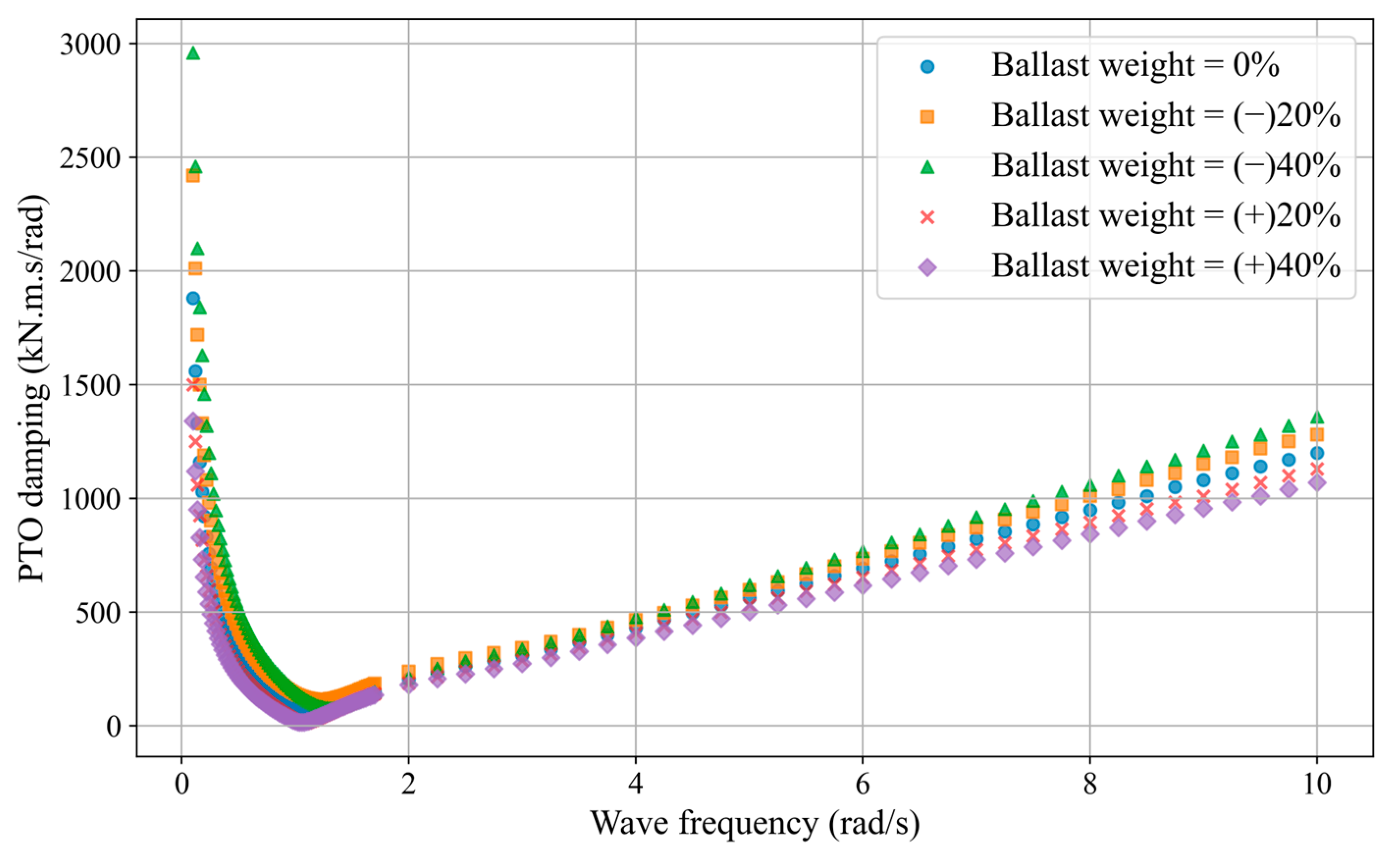
Since the current formulations rely on potential theory, they neglect viscous effects. The estimation of viscosity involves a free decay test conducted using CFD within the Star-ccm+ platform. In these CFD simulations, the fluid dynamics within the designated domain are governed by specific boundary conditions. A fixed domain size of 400 × 5 × 70 m has been chosen, where a 100 m zone on both ends serves as a wave forcing and absorbing zone, acting as a generator and absorber. The remaining part of the domain is designated as a computational zone. A finely detailed mesh is generated near the free surface and WEC rotor, with a gradual increase in mesh size from fine to coarse. A prism layer mesh, with a first cell size of 0.002 m, is created around the WEC rotor to accurately capture the viscous boundary layer. With the exception of the top, which functions as a pressure outlet, all other boundaries are specified as velocity inlets. The WEC rotor is initially positioned at an angle of −20 degrees and allows movement solely in the pitch direction. The mesh around the WEC rotor employs the overset mesh technique, allowing for dynamic mesh movement. For the calculation of turbulent viscosity, a standard low-Re k-ε turbulent model is employed. Temporal integration utilizes the second-order Euler implicit scheme. Through these free decay tests, the parameter kappa (κ) was acquired from successive peaks and obtained the viscosity damping with $2\kappa \rho g{K}_{55}/{\omega }_N$. Subsequently, the corresponding viscous damping values in kN·m·s/rad were calculated and are presented in Figure 8. A clear observation can be made from the figure that higher viscous damping is notably associated with asymmetric WECs possessing a higher ballast weight percentage. This correlation is evident in Figure 8.

5. Performance Evaluation of Supervised Regression ML Models

In this section, a comprehensive investigation into the performance evaluation of the asymmetric WEC with each supervised regression ML model has been conducted. As previously outlined in the data preparation (Section 4), the input dataset encompasses various parameters. These parameters include the variation in ballast weight percentage (ranging from 0%, (+)20%, (+)40%, (−)20%, and (−)40%), along with the positions of the ballast weight in the x- (X_p) and z-directions (Z_p), viscosity damping (B_vis), optimal PTO damping (${\tilde{B}}_{PTO}^{}$), and wave frequency (ω). For a comprehensive overview of the input data’s attributes, the details are succinctly summarized in Table 2. This table presents essential statistical measures, such as mean, standard deviation (STD), and minimum (Min.), as well as the 25th, 50th (median), and 75th percentiles. Notably, the mean and STD values of the optimal extracted power are approximately 25.723 and 38.035 kW/m², respectively, providing a fundamental baseline understanding. An insightful perspective emerges when delving into the percentiles associated with the input data parameters. The percentiles of 25%, 50%, and 75% in relation to the optimal extracted power delineate values of 3.921, 14.581, and 30.276, respectively, tabulated in

Table 3. Summary statistics of input data generated from various asymmetric WEC configurations.

	Ballast (%) Original Weight	xp (m)	zp (m)	Bvis (kN·m·s/rad)	${\tilde{\mathit{B}}}_{\mathit{P}\mathit{T}\mathit{O}}^{}$(kN·m·s/rad)	ω (rad/s)	Power (kW/m2)
Count	2850
Mean	0.00	−1.7790	1.5845	72.930	61.010	2.376	25.723
STD	28.29	0.9879	1.4572	48.308	40.383	2.674	38.035
Min.	(−)40.00	−3.0937	−0.7100	8.813	6.953	0.100	0.001
25%	(−)20.00	−2.0630	0.3962	27.640	18.810	0.660	3.921
50%	0.00	−1.9980	1.6150	57.079	46.043	1.230	14.581
75%	(+)20.00	−1.8521	2.8479	114.850	100.710	3.000	30.276

. These percentile values provide a context for understanding the distribution and variability of the input parameters concerning the optimal power extraction, paving the way for a comprehensive performance evaluation of the adopted ML models.

To assess the hyperparameters of the supervised regression ML models and their impact, the present study considers two scenarios: the first involves the model without hyperparameter tuning (means default values), and the second scenario integrates hyperparameter tuning, as elaborated in Section 3. The essential hyperparameters corresponding to each supervised regression ML model have been detailed in Table 1. In this study, the methodology employs GridSearchCV in conjunction with a five-fold CV. This implies that for each set of hyperparameters associated with each supervised model, the training and evaluation process will be repeated five times. During each iteration, a distinct fold will be designated for testing, while the remaining folds will serve for training. The performance metrics for every combination of hyperparameters will be averaged across the five rounds, as detailed and illustrated in Figure 4. This meticulous strategy ensures that the selection of hyperparameters is not influenced by the performance of a single test set. Instead, it relies on a more consistent and broad evaluation encompassing different data folds. This approach is particularly effective in minimizing the impact of random discrepancies in data division. By incorporating cross-validation, the risk of overfitting to specific dataset partitions is mitigated, enhancing the reliability of assessing how effectively your model generalizes to unseen data. Ultimately, the optimal combinations of hyperparameters that yield favorable scores are given in Table 1.

In the context of the present study, one of the most crucial steps involves the evaluation of ML models to assess their performance on unseen or generalized data. This evaluation is carried out both with and without (default) hyperparameter tuning, as detailed in Table 1. To gain insights into the ML models’ performance, we utilize true vs. predicted curves, as illustrated in Figure 9. Upon a qualitative examination of these figures, a clear pattern emerges: the models with tuned hyperparameters consistently outperform their counterparts without tuning, regardless of the specific ML model being considered. For instance, the SVR model with default hyperparameter settings exhibits comparatively poorer performance, as depicted in Figure 9b left. Within the context of the provided data for the asymmetric WEC, it is evident that the hyperplane identification described in Section 2.2 performs poorly, regardless of whether or not hyperparameters are tuned. The kernel, degree, gamma, C, and ε hyperparameter values of the SVR model exhibit the highest and lowest RMSE and R² values when compared to other ML models. Upon a closer examination of the hyperparameter-tuned ML and XGBoost models, it becomes clear that they demonstrate significantly enhanced performance compared to those with default hyperparameter values. Notably, a visual inspection of the results indicates that the XGBoost model consistently performs exceptionally well in comparison to the other two models. In addition to qualitative observations, we employ quantitative metrics, specifically mean absolute error (MAE), root mean squared error (RMSE), and R², to comprehensively assess the performance of the three models. Detailed quantitative results are presented in

Table 4. Performance quantification of the ML models.

Hyperparameters/ML Models	Supervised Regression ML Models
	MLP	SVR	XGBoost
Default	RMSE: 152.44	RMSE: 152.288	RMSE: 205.9426
	R2: 0.8779	R2: 0.7095	R2: 0.8524
	MAE: 6.529	MAE: 7.9252	MAE: 9.023
Tunned	RMSE: 128.9498	RMSE: 190.1399	RMSE: 5.758
	R2: 0.921576	R2: 0.85170	R2: 0.995106
	MAE: 5.150179	MAE: 4.75838	MAE: 1.21736

. These metrics provide a numerical perspective on the models’ accuracy, error magnitude, and ability to explain variance in the data. The bold text in Table 4 indicates the superior performance among the selected ML models.

Table 4 provides a comprehensive overview of the performance of the ML models in the context of the asymmetric WEC studied here. When considering the default hyperparameter settings, it is evident that the RMSE values are notably higher than the MAE values for all ML models. This discrepancy suggests that predictions made by the MLP, SVR, and XGBoost models tend to have larger errors, with RMSE highlighting these errors more prominently. In terms of the R² score, the MLP model stands out with a high value close to 0.878, indicating a relatively good ability to explain variance in the data compared to the other models. However, when examining the ML models with tuned hyperparameters, a different picture emerges. XGBoost stands out as the superior performer, demonstrating impressive results with an RMSE of 5.758, MAE of 1.217, and an R² score of 0.995. The notably lower difference between RMSE and MAE for XGBoost compared to the other models suggests that it provides more consistent and accurate predictions. Furthermore, it is worth noting that the total number of fits executed using various combinations of hyperparameters for XGBoost amounts to 1500, which is significantly less than the other two ML and SVR models, both of which involve more than 13,440 and 40,320 fits, respectively (Table 1). Also, the high R² score for XGBoost indicates that its predicted values exhibit less variance compared to the true values. This observation aligns with what can be visually confirmed in Figure 9c right, where the predictive performance of XGBoost is evident.

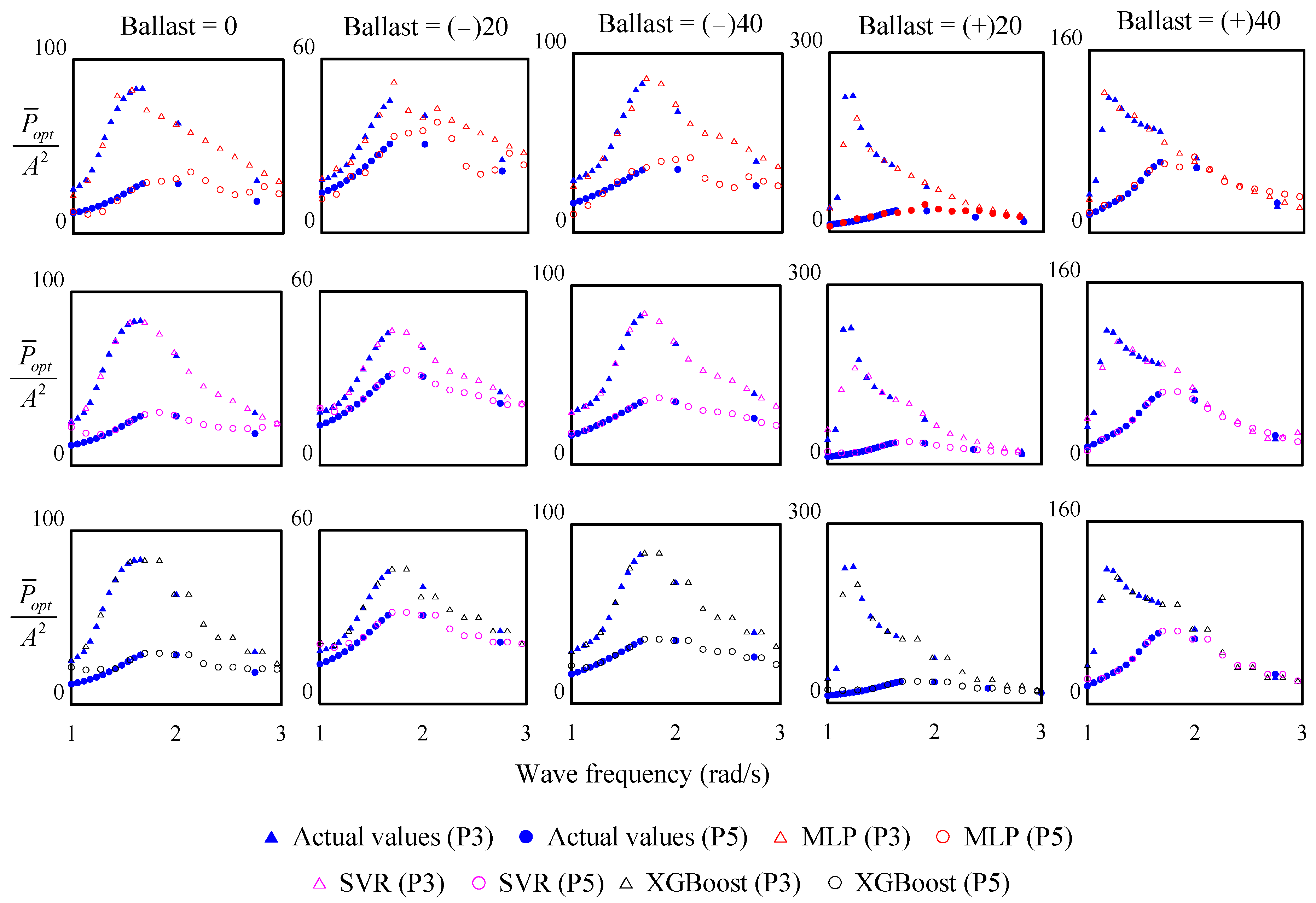
A direct comparison between the actual and predicted (ML models—with tuned hyperparameters) values of optimal power extracted from the WEC is also presented in Figure 10. It is evident that the XGBoost predictions closely align with the actual values derived from the potential model. The required trends, peak values, and low values by the actual model show strong agreement with the predicted values. In light of these findings, it is reasonable to conclude that, based on this study, XGBoost with tuned hyperparameters emerges as the superior choice for predicting the performance of the asymmetric WEC. Furthermore, it is proposed that XGBoost be employed for further investigations, particularly for optimizing the performance of the asymmetric WEC, given its demonstrated strength in this context.

5.1. XGBoost Driven WEC Design Optimization

The trained XGBoost model is now used to investigate for the purpose of optimizing the asymmetric WEC, focusing on the essential parameters detailed in Section 4. To expand this analysis, the study has transitioned from a limited dataset of WECs to employing Latin Hypercube Sampling (LHS), a method designed to efficiently generate a representative set of parameter values from a multidimensional probability distribution. In this endeavor, LHS has been utilized to create 10,000 distinct WECs, encompassing a wide spectrum of extreme input variable values (Ballast weight %: −40 to 40 m; X_P: −3.094 to 1.819 m; Z_P: −0.71 to 4.146 m; B_Vis: 8.813 to 143.690 kN·m·s/rad; ${\tilde{B}}_{PTO}^{}$: 6.953 to 124.750 kN·m·s/rad; and ω : 0.1 to 4 rad/s). An integral feature of LHS is its ability to ensure diversity and an even distribution of sampled values among the generated WECs. Unlike traditional random sampling, where each parameter is selected randomly and independently from a uniform distribution, LHS addresses this limitation by dividing the parameter space into equally likely intervals across each dimension. This stratified approach allows for the creation of bins, with the number of bins aligning with the specified sample size.

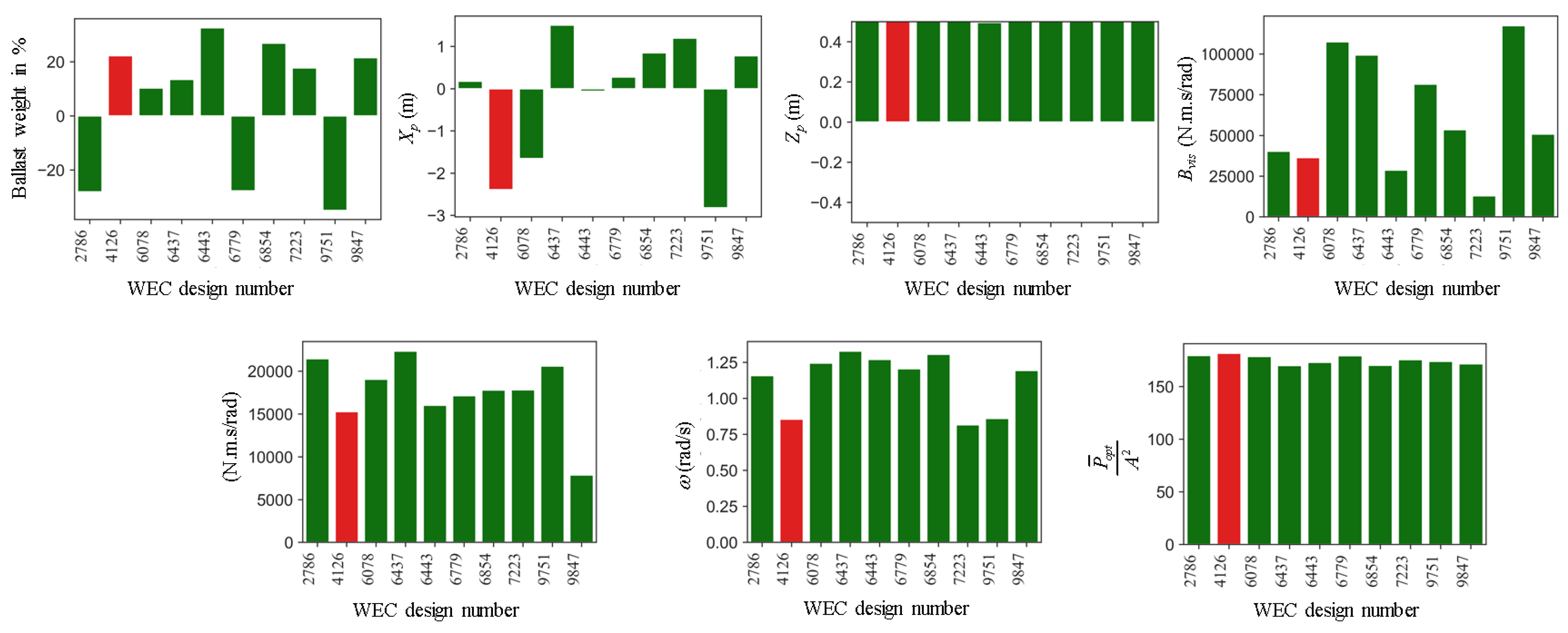
Figure 11 presents the optimal combination of design parameters for the asymmetric WEC, which has been highlighted in red. This optimal configuration is characterized by a ballast weight set at 22.27% of the original, positioned at coordinates of −2.39 m in the x-direction and 3.82 m in the z-direction. Additionally, the viscosity parameter is optimized to 36.437 kN·m·s/rad, and the ideal PTO value is determined to be 15.281 kN·m·s/rad. These parameters are calibrated for a wave frequency of 0.856 rad/s, resulting in an optimal extracted power of 181.603 kW/m². To assess the performance of the asymmetric WEC under these optimized conditions, further simulations are conducted using the potential model, specifically tailored for the desired test site location.

5.2. Irregular Wave Analysis

The test site is located on the western coast of Jeju, South Korea, with coordinates at Latitude 33°19’40.7” N and Longitude 126°08’08.9” E. The wave conditions at this test site have been meticulously characterized using open-source data available on wink.go.kr. These wave conditions, spanning from 1 January 1979 to 9 September 2008, are succinctly constructed in a wave scatter diagram. In this wave scatter diagram, each data point corresponds to specific wave conditions observed at distinct locations and times. These data points are a result of combining two critical parameters: significant wave height (H_s) and peak wave period (T_p). 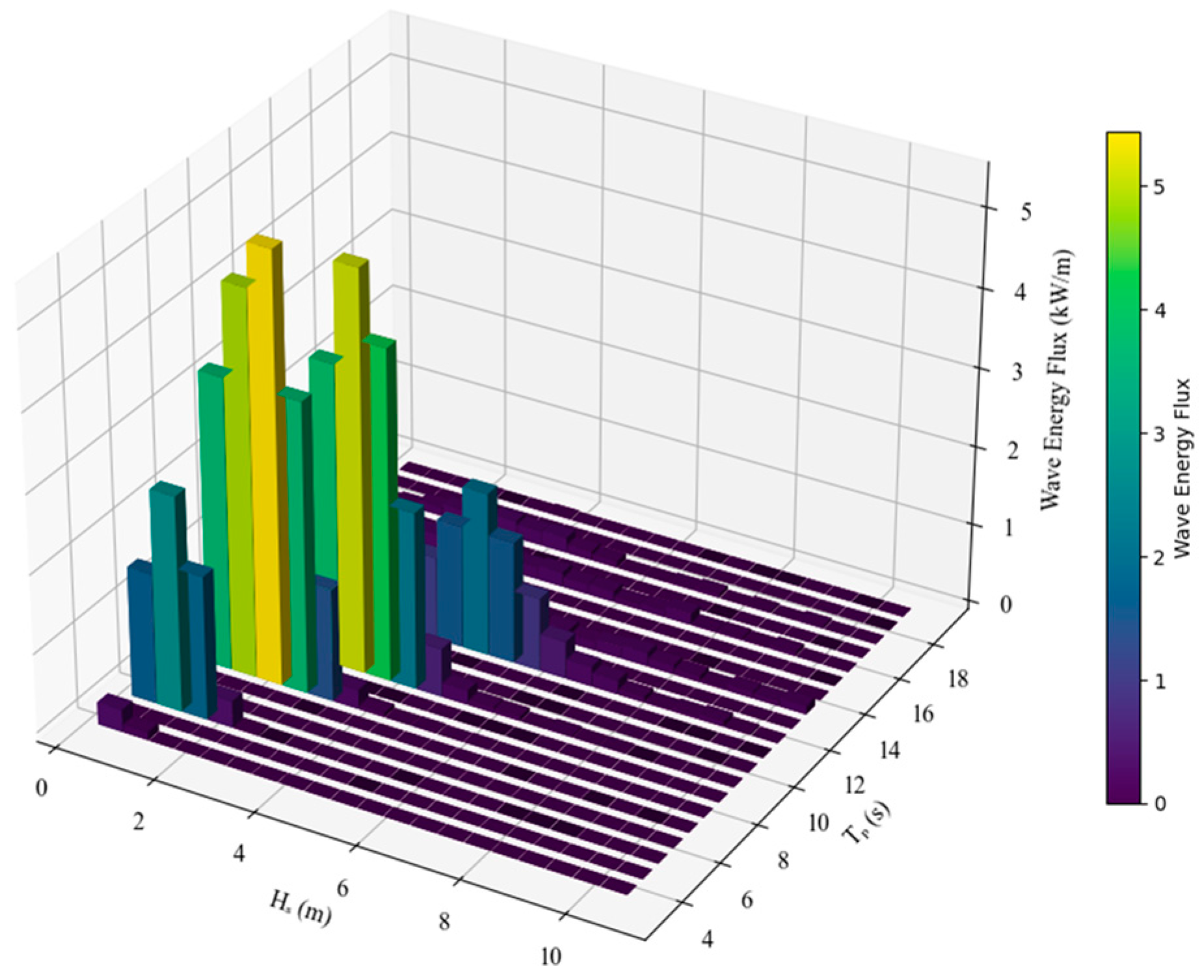Figure 12 supplements this by showcasing the wave energy flux, expressed in watts per meter (W/m) of wavefront, calculated using the formula ($0.5\rho g{H}_s^2{T}_p$), where ρ represents density, and g stands for gravitational acceleration. The wave energy flux is depicted over a range of H_s values from 0.5 m to 10 m, with increments of 0.5 m, including 0.125 m, and T_p ranging from 3 s to 19 s, incremented by 2 s. Notably, Figure 12 reveals a concentrated distribution of wave energy flux within the specific range of H_s from 0.125 m to 2 m and T_p from 3 s to 13 s. This range encompasses 99% of the entire dataset, signifying its significance in the analysis. Consequently, for in-depth investigations, only wave conditions falling within the H_s range of 0.125 m to 2 m and the T_p range of 3 s to 13 s are considered. These selected conditions serve as the basis for estimating the annual power output utilizing the optimized asymmetric WEC, providing a more focused and relevant dataset for further study.

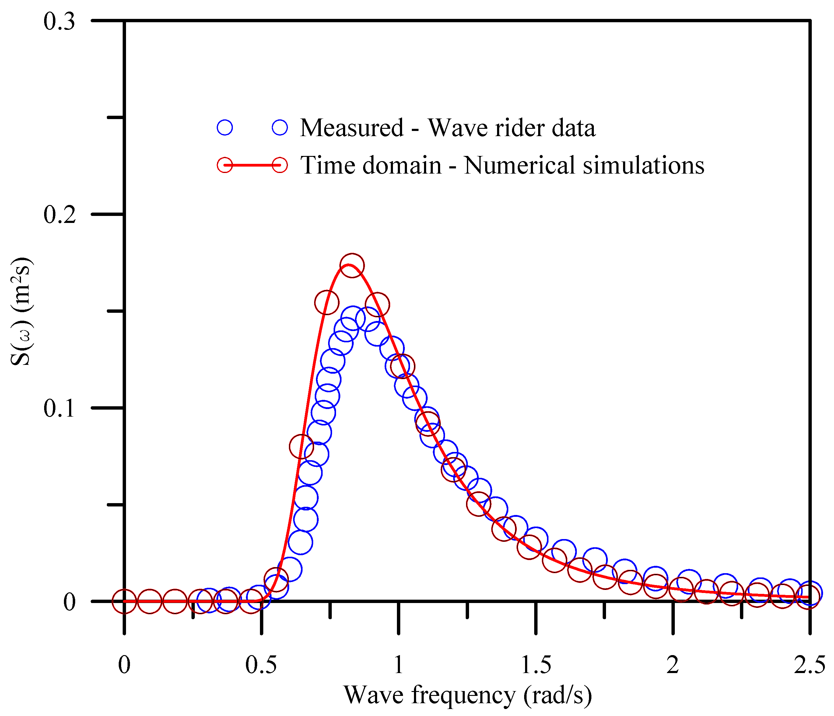
To appropriately model the generation of irregular waves, we have selected specific wave conditions corresponding to a significant wave height (H_s) of 1.26 s and a peak wave period (T_p) of 7.69 s. These conditions were observed during the period from 9 February 2018 to 30 May 2018, at our test location. For simulation purposes, we have used the JONSWAP spectrum with a peakedness factor of one. This simulated results of the WEC whose spectral density (S(ω)) was compared with measured data, and the comparison yielded satisfactory results (see Figure 13). For all other sea state conditions, we have maintained a constant peakedness value of one in the analytical model. This ensures consistency in the simulations. 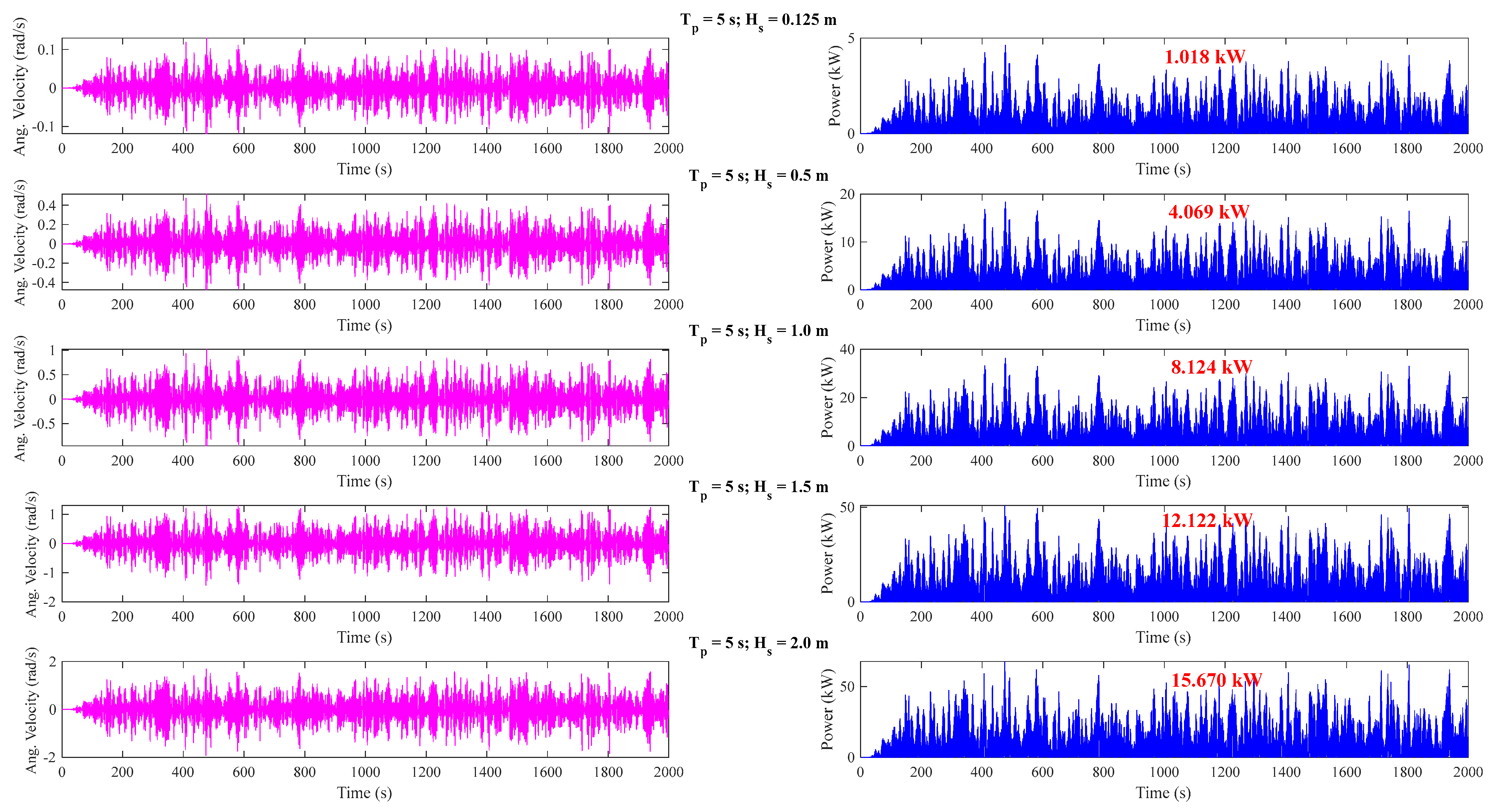When analyzing simulations with varying H_s (from 0.125 m to 2.0 m) and a fixed T_p of 5 s, as depicted in Figure 14, it becomes evident from the figure that as H_s increases, the extracted power also increases rapidly. Specifically, at H_s = 0.125 m, the extracted power reaches 1.018 kW, while at H_s = 2.0 m, it reaches 15.670 kW. 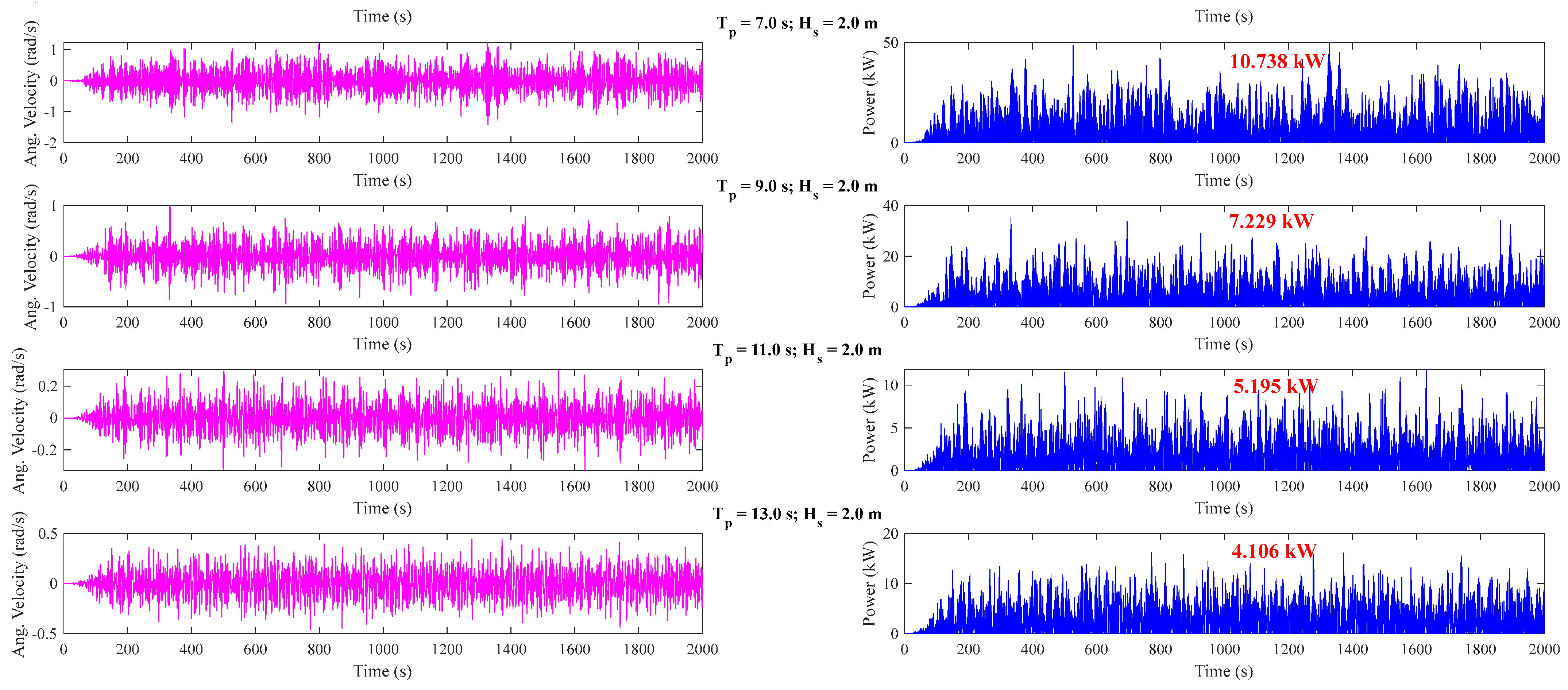Furthermore, in Figure 15, the estimated angular velocity and power for a fixed H_s and T_p variation from 7.0 s to 13 s are shown. Here, as T_p increases, the extracted power decreases. The minimum power of 4.106 kW occurs at T_p = 13 s, while it is 10.738 kW at T_p = 7 s.

Table 5. Mechanical power extraction (kW) from the asymmetric WEC at the test site location.

	Hs (m)	0.125	0.5	1	1.5	2	2.5	3	3.5	4	Sum	Prop. [%]
Tp (s)
13		0.000	0.002	0.006	0.007	0.006	0.007	0.006	0.003	0.002	0.040	0.72
11		0.000	0.007	0.014	0.017	0.010	0.008	0.009	0.014	0.018	0.098	1.78
9		0.001	0.025	0.041	0.068	0.088	0.121	0.134	0.093	0.042	0.613	11.16
7		0.006	0.252	0.568	0.500	0.415	0.221	0.069	0.010	0.002	2.042	37.21
5		0.031	1.059	0.880	0.390	0.053	0.002				2.414	44.00
3		0.017	0.224	0.041	0.000						0.281	5.13
Sum		0.054	1.569	1.550	0.982	0.572	0.360	0.218	0.119	0.065	5.487
Prop. [%]		0.98	28.59	28.25	17.89	10.42	6.56	3.97	2.17	1.18

provides the average mechanical power, which is determined by multiplying the extracted average power with the frequency of occurrence for each sea state. Notably, over 91% of the total energy is concentrated in the range of H_s from 0.5 m to 2.5 m, with corresponding T_p values ranging from 5 s to 9 s. The total mechanical extracted power for the selected wave conditions is found to be 5.487 kW (represented in red color see Table 5). In order to obtain the average extracted power output from the wave scatter diagram, it is necessary to multiply it by a conversion efficiency factor of 0.8. Furthermore, for estimating the annual energy production (AEP), we use a Julian year with 8766 h, an operational efficiency of 0.95, and a transmission efficiency of 0.98. The calculated AEP is found to be 35.83 MW. These results provide crucial insights into the power generation potential of the optimum asymmetric WEC system under different sea state conditions, aiding in the assessment of its overall performance and feasibility.

6. Conclusions

This paper investigates the significance of employing supervised regression ML models in optimizing the design of an asymmetric WEC, aimed at enhancing the WEC’s performance. The WEC design optimization utilizes ML models, including MLP regression, SVR, and XGBoost methods. To identify the optimal parameters for each ML model, hyperparameter optimization is conducted, and the results are compared across the models. To find the optimal asymmetric WEC, LHS is employed to generate 10,000 distinct WEC configurations, encompassing a wide range of extreme input variable values while ensuring diversity and even distribution among the sampled values. Furthermore, a supplementary analysis is carried out to evaluate the WEC’s performance at the designated deployment site. The following conclusions drawn from this study are listed below:

• Default hyperparameters in asymmetric WEC ML models yield higher RMSE values compared to MAE values, with MLP model outperforming other models with an R² score of approximately 0.878.
• Tuned hyperparameters reveal XGBoost as superior in performance with an RMSE of 5.758, MAE of 1.217, and an R² score of 0.995. Predicted XGBoost results align well with actual values.
• Within the tested range of input conditions, the optimal configuration for the asymmetric WEC was identified, featuring a ballast weight set at 22.27%, coordinates at −2.39 m (x-direction) and 3.82 m (z-direction), a viscosity parameter of 36.437 kN·m·s/rad, and an optimal PTO value of 15.281 kN·m·s/rad. This configuration resulted in an optimal power extraction of 181.603 kW/m².
• When observed in irregular waves, the extracted average power increases as H_s increases for a fixed T_p, and conversely, it decreases with a fixed H_s as T_p increases.
• The optimized asymmetric WEC at the test site location achieves an estimated AEP of 35.83 MW.

This study offers essential insights into the power generation potential of the optimized asymmetric WEC system, designed using supervised regression ML models. These insights contribute to assessing the system’s overall performance and feasibility in regular and irregular waves. Future research will extend the application of these ML models to evaluate their performance on multiple WECs on a floating platform.