
An Improved A-Star Ship Path-Planning Algorithm Considering Current, Water Depth, and Traffic Separation Rules


Abstract
1. Introduction
- (1)
- By analyzing the key factors that impact the safe navigation of ships, this paper establishes a risk model that comprehensively considers factors such as water current, water depths, and obstacle distances. The model aims to reduce the risk of collision with obstacles and prevent grounding.
- (2)
- This paper quantifies the traffic separation rules to establish a traffic model. The model enables the ship to adhere to traffic separation rules, reducing the risk of collision with incoming ships.
- (3)
- This paper proposes a turn model and a smooth method to enhance the smoothness of the path. The model optimizes the path on the basis of the ship’s minimum turning radius to make it easier for the ship to track.
2. Literature Review
2.1. Research Progress of Ship Path Planning
2.2. Research Progress of A-Star Algorithm
3. Model Design
3.1. Overview of the Model
3.2. Risk Model
3.3. Traffic Model
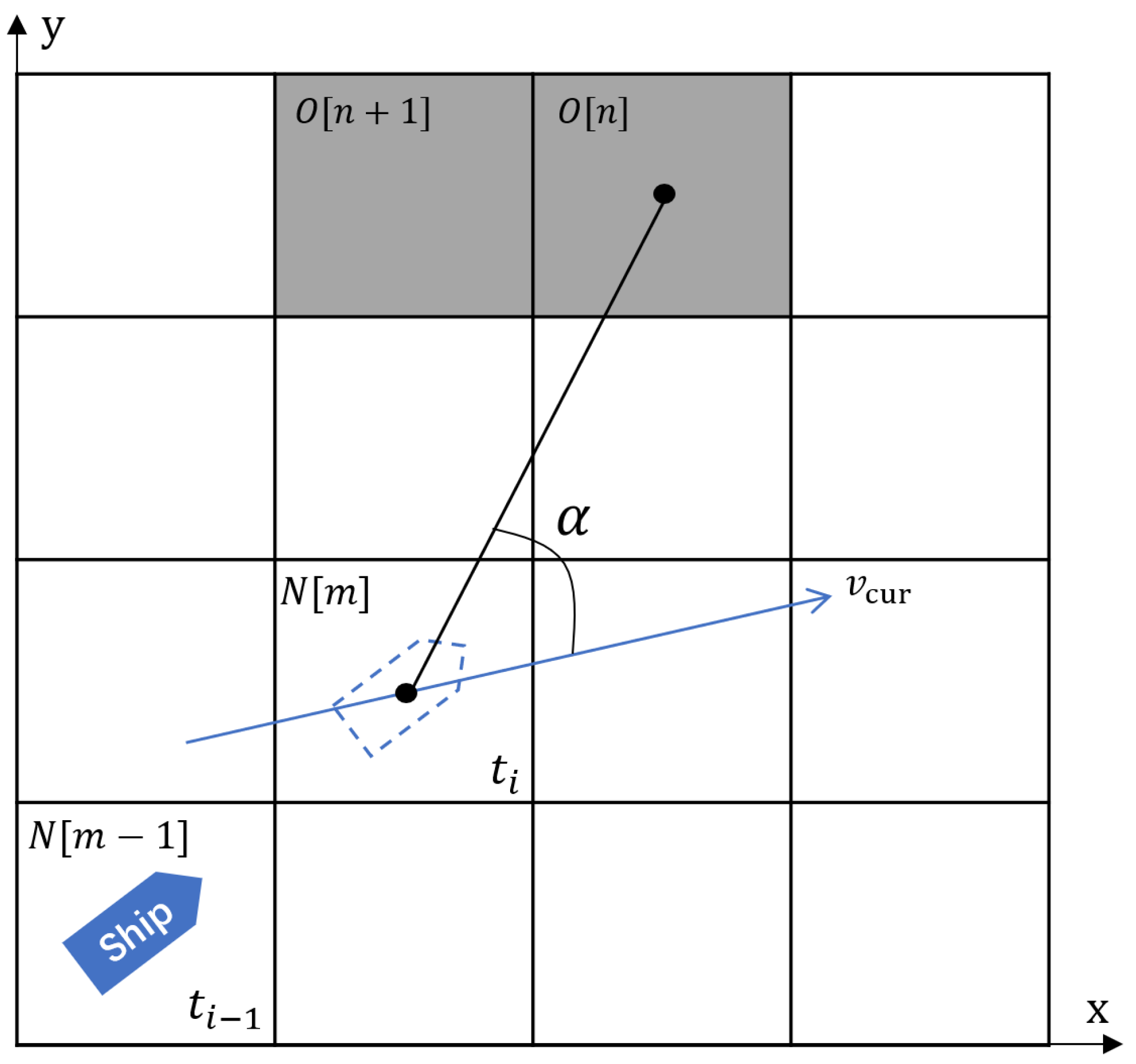
3.4. Turn Model
4. A-Star Algorithm and Improvements
4.1. Environment Modeling
- (1)
- Water area and water depth division standard
- (2)
- Movement rules of ships in the grid environment
4.2. Improved A-Star Algorithm
4.2.1. Traditional A-Star Algorithm
4.2.2. Improved A-Star Algorithm
| Algorithm 1: Improved A-star algorithm | |
| 1: | Mark N[start] as openlist |
| 2: | if not traffic separation rule then |
| 3: | rtra = 0 at any time |
| 4: | While openlist do |
| 5: | Select openlist N[i] whose value of Fn[i] is the smallest |
| 6: | if N[i]=N[goal] then |
| 7: | return “path Pn is found” |
| 8: | else |
| 9: | Mark N[i] as closelist |
| 10: | if successor Ni[j] of N[i] not in closelist or openlist then |
| 11: | Mark Ni[j] as openlist |
| 12: | Calculate rs(j), rtra(j), rturn(j) by (1), (7), and (8), respectively. |
| 13: | if Ni[j] in openlist and Fnew(Ni[j]) is smaller than Fold(Ni[j]) then |
| 14: | Fold(Ni[j]) = Fnew(Ni[j]) and set parent node of N[j] as N[i] |
| 15: | return “path Pn is not found” |
4.2.3. Smooth Paths with Geometry
5. Case Study
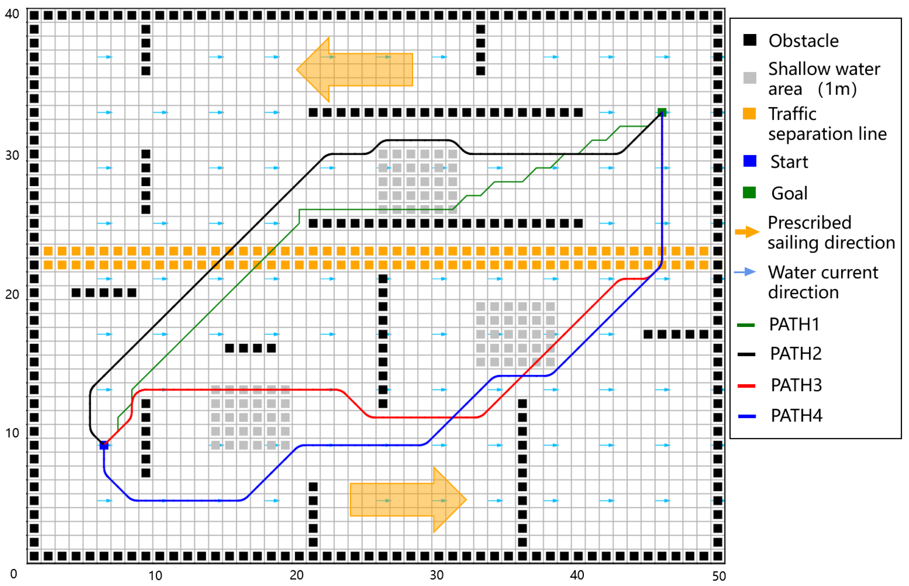
5.1. Case 1: Path Planning in Complex Simulation Environment
5.1.1. Setup
5.1.2. Results
5.2. Case 2: Path Planning in Real Scenes in Zhoushan Port
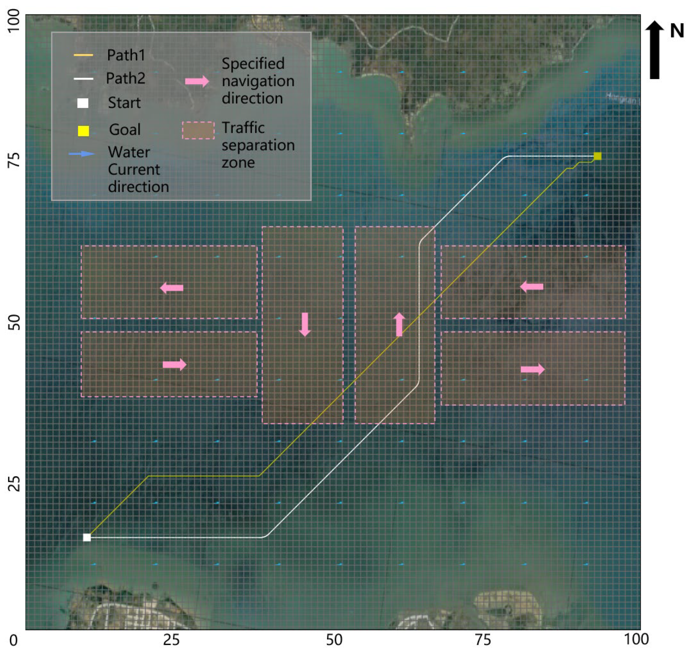
5.3. Case 3: Path Planning in Real Scenes in Hainan Port
6. Conclusions
Author Contributions
Funding
Institutional Review Board Statement
Informed Consent Statement
Data Availability Statement
Conflicts of Interest
References
- Silveira, P.; Teixeira, A.; Figueira, J.R.; Soares, C.G. A multicriteria outranking approach for ship collision risk assessment. Reliab. Eng. Syst. Saf. 2021, 214, 107789. [Google Scholar] [CrossRef]
- Liu, J.; Yan, X.; Liu, C.; Fan, A.; Ma, F. Developments and Applications of Green and Intelligent Inland Vessels in China. J. Mar. Sci. Eng. 2023, 11, 318. [Google Scholar] [CrossRef]
- Jorge, V.A.M.; Granada, R.; Maidana, R.G.; Jurak, D.A.; Heck, G.; Negreiros, A.P.F.; dos Santos, D.H.; Goncalves, L.M.G.; Amory, A.M. A Survey on Unmanned Surface Vehicles for Disaster Robotics: Main Challenges and Directions. Sensors 2019, 19, 702. [Google Scholar] [CrossRef] [PubMed]
- Wang, L.; Li, S.; Liu, J.; Hu, Y.; Wu, Q. Design and implementation of a testing platform for ship control: A case study on the optimal switching controller for ship motion. Adv. Eng. Softw. 2023, 178, 103427. [Google Scholar] [CrossRef]
- Felski, A.; Zwolak, K. The ocean-going autonomous ship—Challenges and threats. J. Mar. Sci. Eng. 2020, 8, 41. [Google Scholar] [CrossRef]
- Zhen, R.; Shi, Z.; Liu, J.; Shao, Z. A novel arena-based regional collision risk assessment method of multi-ship encounter situation in complex waters. Ocean Eng. 2022, 246, 110531. [Google Scholar] [CrossRef]
- Wang, N.; Sun, Z.; Yin, J.; Zou, Z.; Su, S.-F. Fuzzy unknown observer-based robust adaptive path following control of underactuated surface vehicles subject to multiple unknowns. Ocean Eng. 2019, 176, 57–64. [Google Scholar] [CrossRef]
- Zhen, R.; Shi, Z.; Shao, Z.; Liu, J. A novel regional collision risk assessment method considering aggregation density under multi-ship encounter situations. J. Navig. 2022, 75, 76–94. [Google Scholar] [CrossRef]
- Zhou, C.; Gu, S.; Wen, Y.; Du, Z.; Xiao, C.; Huang, L.; Zhu, M. The review unmanned surface vehicle path planning: Based on multi-modality constraint. Ocean Eng. 2020, 200, 107043. [Google Scholar] [CrossRef]
- Li, S.; Xu, C.; Liu, J.; Han, B. Data-driven docking control of autonomous double-ended ferries based on iterative learning model predictive control. Ocean Eng. 2023, 273, 113994. [Google Scholar] [CrossRef]
- Liu, J.; Wang, J. Overview of obstacle avoidance path planning algorithms for unmanned surface vehicle. Comput. Appl. Softw. 2020, 37, 1–10+20. [Google Scholar]
- Cheng, T.; Utne, I.B.; Wu, B.; Wu, Q. A novel system-theoretic approach for human-system collaboration safety: Case studies on two degrees of autonomy for autonomous ships. Reliab. Eng. Syst. Saf. 2023, 237, 109388. [Google Scholar] [CrossRef]
- Chen, X.; Liu, S.; Liu, R.W.; Wu, H.; Han, B.; Zhao, J. Quantifying Arctic oil spilling event risk by integrating an analytic network process and a fuzzy comprehensive evaluation model. Ocean Coast. Manag. 2022, 228, 106326. [Google Scholar] [CrossRef]
- Liu, Z.; Zhang, Y.; Yu, X.; Yuan, C. Unmanned surface vehicles: An overview of developments and challenges. Annu. Rev. Control 2016, 41, 71–93. [Google Scholar] [CrossRef]
- Chen, X.; Wu, S.; Shi, C.; Huang, Y.; Yang, Y.; Ke, R.; Zhao, J. Sensing data supported traffic flow prediction via denoising schemes and ANN: A comparison. IEEE Sens. J. 2020, 20, 14317–14328. [Google Scholar] [CrossRef]
- Liu, Y.C.; Bucknall, R. Path planning algorithm for unmanned surface vehicle formations in a practical maritime environment. Ocean Eng. 2015, 97, 126–144. [Google Scholar] [CrossRef]
- Singh, Y.; Sharma, S.; Sutton, R.; Hatton, D.; Khan, A. Feasibility study of a constrained Dijkstra approach for optimal path planning of an unmanned surface vehicle in a dynamic maritime environment. In Proceedings of the 2018 IEEE International Conference on Autonomous Robot Systems and Competitions (ICARSC), Torres Vedras, Portugal, 25–27 April 2018; pp. 117–122. [Google Scholar]
- Liang, C.L.; Zhang, X.K.; Watanabe, Y.; Deng, Y.J. Autonomous Collision Avoidance of Unmanned Surface Vehicles Based on Improved a Star and Minimum Course Alteration Algorithms. Appl. Ocean Res. 2021, 113, 102755. [Google Scholar] [CrossRef]
- Gu, Q.; Zhen, R.; Liu, J.; Li, C. An improved RRT algorithm based on prior AIS information and DP compression for ship path planning. Ocean Eng. 2023, 279, 114595. [Google Scholar] [CrossRef]
- Chi, W.; Ding, Z.; Wang, J.; Chen, G.; Sun, L. A Generalized Voronoi Diagram-Based Efficient Heuristic Path Planning Method for RRTs in Mobile Robots. IEEE Trans. Ind. Electron. 2021, 69, 4926–4937. [Google Scholar] [CrossRef]
- Dong, Y.; Camci, E.; Kayacan, E. Faster RRT-based nonholonomic path planning in 2D building environments using skeleton-constrained path biasing. J. Intell. Robot. Syst. 2018, 89, 387–401. [Google Scholar] [CrossRef]
- Cao, S.; Fan, P.; Yan, T.; Xie, C.; Deng, J.; Xu, F.; Shu, Y. Inland waterway ship path planning based on improved RRT algorithm. J. Mar. Sci. Eng. 2022, 10, 1460. [Google Scholar] [CrossRef]
- Öztürk, Ü.; Akdağ, M.; Ayabakan, T. A review of path planning algorithms in maritime autonomous surface ships: Navigation safety perspective. Ocean Eng. 2022, 251, 111010. [Google Scholar] [CrossRef]
- Lin, H.X.; Xiang, D.; Ou, Y.J.; Lan, X.D. Review of Path Planning Algorithms for Mobile Robots. Comput. Eng. Appl. 2021, 57, 38–48. [Google Scholar]
- Long, Y.; Su, Y.; Zhang, H.; Li, M. Application of improved genetic algorithm to unmanned surface vehicle path planning. In Proceedings of the 2018 IEEE 7th Data Driven Control and Learning Systems Conference (DDCLS), Enshi, China, 25–27 May 2018; pp. 209–212. [Google Scholar]
- Zhang, J.; Chen, X.; Hu, H.; Zhang, J.; Wang, L. Global path planning algorithm based on the IPSO algorithm for USVs. In Proceedings of the 2018 Chinese Control and Decision Conference (CCDC), Shenyang, China, 9–11 June 2018; pp. 4901–4906. [Google Scholar]
- Woo, J.; Kim, N. Collision avoidance for an unmanned surface vehicle using deep reinforcement learning. Ocean Eng. 2020, 199, 107001. [Google Scholar] [CrossRef]
- Li, L.; Wu, D.; Huang, Y.; Yuan, Z.-M. A path planning strategy unified with a COLREGS collision avoidance function based on deep reinforcement learning and artificial potential field. Appl. Ocean Res. 2021, 113, 102759. [Google Scholar] [CrossRef]
- Liu, Z.; Zhou, Z.Z.; Zhang, M.Y.; Liu, J.X. A Twin Delayed Deep Deterministic Policy Gradient Method for Collision Avoidance of Autonomous Ships. J. Transp. Inf. Saf. 2022, 40, 60–74. [Google Scholar]
- Ayawli, B.B.K.; Chellali, R.; Appiah, A.Y.; Kyeremeh, F. An Overview of Nature-Inspired, Conventional, and Hybrid Methods of Autonomous Vehicle Path Planning. J. Adv. Transp. 2018, 8269698. [Google Scholar] [CrossRef]
- Guo, B.; Kuang, Z.; Guan, J.; Hu, M.; Rao, L.; Sun, X. An Improved A-Star Algorithm for Complete Coverage Path Planning of Unmanned Ships. Int. J. Pattern Recognit. Artif. Intell. 2022, 36, 2259009. [Google Scholar] [CrossRef]
- Duchon, F.; Babinec, A.; Kajan, M.; Beno, P.; Florek, M.; Fico, T.; Jurisica, L. Path planning with modified A star algorithm for a mobile robot. In Proceedings of the 6th Conference on Modelling of Mechanical and Mechatronic Systems (MMaMS), Vysoke Tatry, Slovakia, 25–27 November 2014; pp. 59–69. [Google Scholar]
- Chen, D.T.; Liu, X.D.; Liu, S.W. Improved A* algorithm based on two-way search for path planning of automated guided vehicle. J. Comput. Appl. 2021, 41, 309–313. [Google Scholar]
- Fernandes, E.; Costa, P.; Lima, J.; Veiga, G. Towards an Orientation Enhanced A star Algorithm for Robotic Navigation. In Proceedings of the IEEE International Conference on Industrial Technology (ICIT), Seville, Spain, 17–19 March 2015; pp. 3320–3325. [Google Scholar]
- Zhang, J.G.; Zhang, F.; Chen, L.G.; Jiang, Q.; Zhu, W. Path planning of automatic guided vehicle based on improved A* algorithm. Foreign Electron. Meas. Technol. 2022, 41, 123–128. [Google Scholar] [CrossRef]
- Zhang, Y.; Li, L.-l.; Lin, H.-C.; Ma, Z.; Zhao, J. Development of Path Planning Approach Based on Improved A-Star Algorithm in AGV System. In Proceedings of the 3rd European-Alliance-for-Innovation (EAI) International Conference on IoT as a Service (IoTaaS), Taichung, Taiwan, 20–22 September 2017; pp. 276–279. [Google Scholar]
- Nayl, T.; Mohammed, M.Q.; Muhamed, S.Q. Obstacles Avoidance for an Articulated Robot Using Modified Smooth Path Planning. In Proceedings of the International Conference on Computer and Applications (ICCA), Doha, United Arab Emirates, 6–7 September 2017; pp. 185–189. [Google Scholar]
- Lu, W.L.; Lei, J.S.; Shao, Y. Path Planning for Mobile Robot Based on an Improved A* Algorithm. J. Ordnance Equip. Eng. 2019, 40, 197–201. [Google Scholar]
- Gunawan, S.A.; Pratama, G.N.; Cahyadi, A.I.; Winduratna, B.; Yuwono, Y.C.; Wahyunggoro, O. Smoothed A-star algorithm for nonholonomic mobile robot path planning. In Proceedings of the 2019 International Conference on Information and Communications Technology (ICOIACT), Yogyakarta, Indonesia, 24–25 July 2019; pp. 654–658. [Google Scholar]
- Sun, J.G.; Sun, T. Research on UAV path planning based on fusion A* algorithm. Electron. Meas. Technol. 2022, 45, 82–91. [Google Scholar] [CrossRef]
- Shu, W.N.; Zhao, J.S.; Xie, Z.X.; Zhang, X.S.; Ma, X. Path planning for unmanned surface vessels based on improved A* algorithm. J. Shanghai Marit. Univ. 2022, 43, 1–6. [Google Scholar] [CrossRef]
- Liu, C.G.; Mao, Q.Z.; Chu, X.M.; Xie, S. An Improved A-Star Algorithm Considering Water Current, Traffic Separation and Berthing for Vessel Path Planning. Appl. Sci. 2019, 9, 1057. [Google Scholar] [CrossRef]
- Liu, S. Study on the Path Planning Algorithm of Unmanned Surface Vehicles in Complex Marine Environment. Master’s Thesis, Tianjin University, Tianjin, China, 2019. [Google Scholar]
- Lee, T.; Kim, H.; Chung, H.; Bang, Y.; Myung, H. Energy efficient path planning for a marine surface vehicle considering heading angle. Ocean Eng. 2015, 107, 118–131. [Google Scholar] [CrossRef]
- Razgallah, I.; Kaidi, S.; Smaoui, H.; Sergent, P. The impact of free surface modelling on hydrodynamic forces for ship navigating in inland waterways: Water depth, drift angle, and ship speed effect. J. Mar. Sci. Technol. 2019, 24, 620–641. [Google Scholar] [CrossRef]
- Zhang, X.; Zhang, Q.; Yang, J.; Cong, Z.; Luo, J.; Chen, H. Safety Risk Analysis of Unmanned Ships in Inland Rivers Based on a Fuzzy Bayesian Network. J. Adv. Transp. 2019, 2019, 4057195. [Google Scholar] [CrossRef]
- Andersen, P. Ship motions and sea loads in restricted water depth. Ocean Eng. 1979, 6, 557–569. [Google Scholar] [CrossRef]
- Bai, X.E.; Jiang, M.Z.; Xu, X.F.; Sun, D.Y. Ship route planning based on improved ant colony algorithm of two-way search. China Navig. 2022, 45, 13–20. [Google Scholar]
- Wang, Y.; Liang, X.; Li, B.; Yu, X. Research and implementation of global path planning for unmanned surface vehicle based on electronic chart. In Recent Developments in Mechatronics and Intelligent Robotics: Proceedings of the International Conference on Mechatronics and Intelligent Robotics (ICMIR2017); Springer: Berlin/Heidelberg, Germany, 2018; Volume 1, pp. 534–539. [Google Scholar]


| Parameters | Value |
|---|---|
| Ship length | 12.86 m |
| Ship width | 3.8 m |
| Design maximum draft | 1 m |
| Minimum turning radius | 36 m |
| Design velocity | 8 knots |
| Parameters | Value |
|---|---|
| Node range of x-axis | [1, 50] |
| Node range of y-axis | [1, 40] |
| Grid length | 20 m |
| Minimum radius of ship | 36 m |
| 0.2 | |
| 0.5 |
| Path Length (m) | Collision Risk | Turn Times (n) | Compliance with Traffic Separation Rules | |
|---|---|---|---|---|
| Path1 | 516.9 | 30.11 | 19 | No |
| Path2 | 545.2 | 13.53 | 7 | No |
| Path3 | 592.1 | 18.58 | 8 | Yes |
| Path4 | 608.7 | 9.39 | 8 | Yes |
| Path Length (miles) | Turn Times (n) | ||
|---|---|---|---|
| Path1 | 0.52 | inf | 16 |
| Path2 | 0.65 | 21.8 | 4 |
| Path Length (miles) | Turn Times (n) | Compliance with Traffic Separation Rules | ||
|---|---|---|---|---|
| Path1 | 17.38 | inf | 6 | No |
| Path2 | 19.54 | 25.8 | 4 | Yes |
Disclaimer/Publisher’s Note: The statements, opinions and data contained in all publications are solely those of the individual author(s) and contributor(s) and not of MDPI and/or the editor(s). MDPI and/or the editor(s) disclaim responsibility for any injury to people or property resulting from any ideas, methods, instructions or products referred to in the content. |
© 2023 by the authors. Licensee MDPI, Basel, Switzerland. This article is an open access article distributed under the terms and conditions of the Creative Commons Attribution (CC BY) license (https://creativecommons.org/licenses/by/4.0/).
Share and Cite
Zhen, R.; Gu, Q.; Shi, Z.; Suo, Y. An Improved A-Star Ship Path-Planning Algorithm Considering Current, Water Depth, and Traffic Separation Rules. J. Mar. Sci. Eng. 2023, 11, 1439. https://doi.org/10.3390/jmse11071439
Zhen R, Gu Q, Shi Z, Suo Y. An Improved A-Star Ship Path-Planning Algorithm Considering Current, Water Depth, and Traffic Separation Rules. Journal of Marine Science and Engineering. 2023; 11(7):1439. https://doi.org/10.3390/jmse11071439
Chicago/Turabian StyleZhen, Rong, Qiyong Gu, Ziqiang Shi, and Yongfeng Suo. 2023. "An Improved A-Star Ship Path-Planning Algorithm Considering Current, Water Depth, and Traffic Separation Rules" Journal of Marine Science and Engineering 11, no. 7: 1439. https://doi.org/10.3390/jmse11071439
APA StyleZhen, R., Gu, Q., Shi, Z., & Suo, Y. (2023). An Improved A-Star Ship Path-Planning Algorithm Considering Current, Water Depth, and Traffic Separation Rules. Journal of Marine Science and Engineering, 11(7), 1439. https://doi.org/10.3390/jmse11071439