Ship Autonomous Berthing Simulation Based on Covariance Matrix Adaptation Evolution Strategy

Abstract

Existing research on auto-berthing of ships has mainly focused on the design and implementation of controllers for automatic berthing. For the real automatic docking processes, not only do external environmental perturbations need to be taken into account but also motion paths, docking strategies and ship mechanical constraints, which are important influential factors to measure autonomous docking methods. Through a literature review of ship path planning and motion control for automatic berthing, it is found that many studies ignore the interference of the actual navigational environment, especially for ships sailing at slow speed when berthing, or do not consider the physical constraints of the steering gear and the main engine. In this paper, we propose a hybrid approach for autonomous berthing control systems based on a Linear Quadratic Regulator (LQR) and Covariance Matrix Adaptation Evolution Strategy (CMA-ES), which systematically addresses the problems involved in the berthing process, such as path planning, optimal control, adaptive berthing strategies, dynamic environmental perturbations and physically enforced structural constraints. The berthing control system based on the LQR and modified LQR-CMA-ES have been validated by simulation work. The simulation results show that the proposed method is able to achieve the automatic docking of the ship well and the system is robust and well adapted to environmental disturbances at slow speed when docking.

1. Introduction

Accelerating the construction of intelligent, efficient and green marine transportation vessels is one of the methods for developing the marine economy. Unmanned Surface Vehicle (USV) refers to an intelligent ship that can sail autonomously on the water without the participation of crew. Elevated velocity, diminutive dimensions, reduced cost and the ability for autonomous navigation constitute the salient attributes possessed by this kind of watercraft, rendering USVs preferred in manifold scenarios such as open sea search and rescue and military maneuvers. In virtue of the intrinsic properties surrounding the hull, watercraft of such small size are readily maneuvered yet easily affected by disturbances from ambient conditions, thereby imposing relatively strict requirements on the robustness of the kinetic control system.

In 1987, Kose et al. [1] first realized the automatic berthing and unberthing of ships by means of computer-aided control and tug assistance. In 2015, Mizuno et al. [2] proposed a quasi-real-time automatic berthing control method based on a multiple shooting method, which can give a solution in a short time. In 2017, Zhang et al. [3] promulgated a nonlinear feedback algorithm predicated upon a bipolar S-PID, based on the MMG vessel model, which suppressed perturbations and extraneous disturbances during the docking process to maintain the ideal heading for the watercraft and the safety of the berthing procedure. In 2020, Xu et al. [4] proposed a robust adaptive control algorithm to address the perturbations engendered by the bank effect on the berthing control of a vessel and eliminate the oscillatory manifestations in the control outputs. Han [5] promulgated a disturbance rejection control algorithm based on neural networks to accomplish the heading control of vessels with minimal overshoot and effectuate berthing control maneuvers. In 2021, Jia et al. [6] retrained the controller by using an ANN, which improved the accuracy of the output and solved the problem of yaw deviation during berthing. Wang et al. [7] designed the Linear Quadratic Regulator (LQR) controller combined with a GA, which reduced the additional resistance of the system caused by pitch and heave motion.

In 2019, Yang [8] proposed an accelerated evolutionary algorithm based on the Covariance Matrix Adaptation Evolution Strategy (CMA-ES), which reduced the time complexity of the algorithm and solved the issue of premature convergence of multi-objective optimization. In 2020, Maki et al. [9] applied CMA-ES to the optimization of control parameters of an automatic berthing system, and the deviations between the actual trajectory and the predetermined reference path during the berthing maneuver were minimized. In 2021, Maniyappan et al. [10] used the CMA-ES to carry out PD optimal control on the time series of rudder angle change, and the experiments showed that the optimized controller improved the yaw check effectively. In 2022, Miyauchi et al. [11] used the CMA-ES algorithm to optimize the parameters of the Nomoto model which described the ship’s kinematic behavior in the process of berthing and obtained a better control effect by enhanced accuracy.

In

Table 1. Comparison of research on berthing-related papers in recent years.

Core Method	Researchers	Outcome	Experiment
LQR control	Yazdanpanah et al. [12]	The feedback gain of the system was calibrated through the combination of LQR and fuzzy logical control.	Simulation
	Brasel [13]	The heading angle and velocity of the vessel were modulated under disparate operating conditions via LQR.	Simulation
	Shao [14]	The kinetics of an oil tanker was governed within the limited boundary of the channel through an LQR controller.	Simulation
	Farzanegan et al. [15]	The heaving motions of a ship were damped using an LQR regulator.	Simulation
	Tian [16]	The yaw-checking maneuver was optimized under the straight sailing condition by an LQR controller.	Simulation
	Zhao et al. [17]	Based on the LQR, a controller without static error was utilized to achieve heading stabilization.	Simulation
CMA-ES optimization	Chen [18]	The ambulatory kinetics of the robot were optimized.	Simulation
	Maki et al. [9,19,20]	The frequent rudder, propeller operation and control objective function during the berthing process were optimized.	Simulation
	Maniyappan et al. [10]	Global optimization of the rudder control for the yaw checking.	Simulation
	Liu et al. [21]	A synopsis of the technology for automated docking and undocking at the current stage was given.	Simulation
	Akimoto et al. [22]	Antagonistic CMA-ES was used for automatic berthing control with uncertainty.	Simulation
	Miyauchi et al. [23]	A systematic berthing model was constructed and the berthing trajectory was optimized.	Simulation
Other	Jia et al. [6]	The issue of excessive heading deviation was addressed through neural networks by berthing training data.	Simulation
	Homburger et al. [24]	MPPI methodology was utilized to implement berthing control and achieve optimal control in a nonlinear system.	Simulation
	Sawada et al. [25]	An automated berthing control system was propounded and trajectory tracking was performed through numerical simulation.	Simulation
	Zhang et al. [26]	Reinforcement learning based on demonstration data was used for auto-berthing control.	Simulation
	Kamil et al. [27]	An ANN-based controller was proposed to simulate a human brain’s activity during the execution phase.	Simulation
	Xu et al. [28]	A three-phase guidance algorithm was devised to ensure stable operation of the vessel when transient and during berthing.	Simulation

, a synopsis of the research on kinetic control mechanisms and optimization thereof for watercraft, undertaken by a selection of scholars, has been compiled, to serve as the theoretical foundation for subsequent study in this paper.

Automated berthing of vessels has always been an important area in the research of ship navigation automation. Since the automatic berthing of a ship is low-speed maneuvering motion in restricted waters, the interference from the external environment on the maneuver control system cannot be ignored. Although a series of automated measures have been basically realized, including autonomous collision avoidance and route planning, autonomous ship berthing remains a major challenge in the development of intelligent ships at present. The “final one mile” problem of autonomous ships has not yet been well solved, and much research work remains to be carried out.

According to the summation shown in Table 1, LQR demonstrates propitious compatibility which has great facilities in the MIMO control domain, providing a new way to control the complicated docking process of ships. Moreover, the CMA-ES has exhibited efficacious effects on model parameter and control law optimization. The essence of the research is combining a controller with effective compatibility and a robustly effectual optimizer to accomplish autonomous berthing of ships.

The autonomous berthing system architecture proposed in this paper based on the current status of research on automatic berthing of ships is depicted in Figure 1. It encompasses the path planning, optimal control, power distribution and other indicators required for ship intellectualization and can achieve the “final one mile” motion control objective of automatic ship berthing. In

Table 2. Inadequacies in current research and corresponding solutions.

Problems in Current Research	Solutions Given in This Paper
The disturbances of wind and currents are not considered.	The interference with the berthing process is considered.
The mechanical constraints of ship motion are not considered.	The mechanical constraint of rudder and propeller is added to the whole process of ship motion.
PID, robust and fuzzy control are inconspicuous in the MIMO field.	The LQR control method with good performance in MIMO is selected.
The difference in ship mathematical motion models (large drift angle) in the low-speed domain is not considered.	The low-speed large drift angle motion correction model is introduced in the berthing stage.
The overall optimization of the berthing process is not considered.	An architecture of the berthing control system is proposed.

, the problems that have been disregarded or not thoroughly explored in the studies above are summarized, and the corresponding solutions are provided in this paper.

In order to solve the problems existing in the current research, this paper uses the Linear Quadratic Regulator (LQR) as the fundamental control model for the controller according to the requirements of the ship’s auto-berthing in the “Guide to Autonomous Cargo Ships” [29] issued by the China Classification Society in 2018. The output of an LQR controller and the path of ship berthing are optimized by using the Covariance Adaptive Adjustment Evolutionary Strategy (CMA-ES) algorithm. The kinematic modeling of the vessel included the low-speed and high-drift angle ship maneuvering emendation model proposed by Yoshimura Yasuo [30]. To fulfill the real situation during the berthing process, disturbances caused by the wind and current were introduced in the experiments in this paper and a simple navigational chart with isometric scaling was introduced as the test environment.

The organizational structure of this paper is as follows: The first section delineates the relevant research on autonomous ship berthing technology. In the second part, the fundamental ship handling maneuvering model used in this paper is characterized. The third section articulates the LQR controller and CMA-ES optimization strategy, introducing the berthing approach based on the CMA-ES and LQR algorithms. This section also introduces the modified model for low-speed and large drift angle motility to suit authentic simulation experiments on a vessel. In the fourth section, several simulation experiments are described, implementing and validating the efficiency of the proposed methodology and analyzing control effects under different simulation scenarios, while two berthing strategies for different berthing conditions are proposed. Finally, in the fifth part, an encapsulation of the research expounded is summarized.

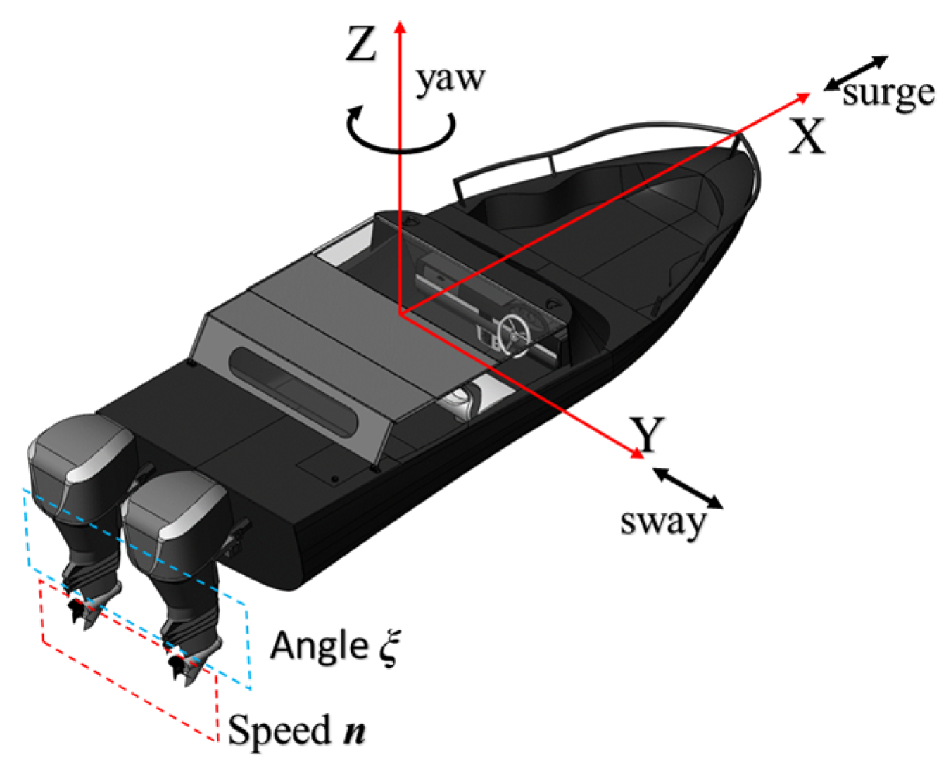
2. Ship Kinematics Model

According to the ship state space model proposed by Fossen [31], the dynamic model of a USV is described in Equation (1), where $\mathbf{\nu }$ and $\eta$ are defined as state vectors describing the linear velocity (or angular velocity) and position (or Euler angle) of the ship in three degrees of freedom, $\tau ={[X,Y,N]}^T$ is the force or moment acting on the ship, $\omega$ is the force or moment acting on the ship by wind and current induced by the environment and $J_{\mathrm{\Theta }}(\eta )$ is the Euler angle rotation matrix. The parameters relevant to this model have been explicated in detail in [31].

$$\begin{array}{r}\mathit{M}\dot{\mathit{\nu }}+\mathit{C}(\mathit{\nu })\mathit{\nu }+\mathit{D}(\mathit{\nu })\mathit{\nu }+\mathit{G}(\eta )=\tau +\omega (t)\\ \dot{\eta }=J_{\mathrm{\Theta }}(\eta )\mathit{\nu }\hspace{1em}\end{array}$$

(1)

For the facilitation of the research endeavors herein, the conventional three degrees of freedom (surge, sway and yaw) ship handling maneuvering model was adopted. Figure 2 delineates the schematic representation of the three degrees of freedom model of the ship utilized. The simplified three degrees of freedom do not consider the restoring force, thus,$G(\eta )=0$. At the same time, the influence of wind and current is added to the model, and the three degrees of freedom ship model is finally expressed as Equation (2), where ${\mathit{\tau }}_{\mathrm{wind}}$ and ${\mathit{\tau }}_{\mathrm{current}}$ correspond to the force or moment of wind and current acting on the ship, respectively, ${\mathit{V}}_c=J_{\mathrm{\Theta }}(\eta ){\mathit{\nu }}_c$ is the current speed in the navigation coordinate system (NED coordinate system), ${\mathit{\nu }}_r$ is the ship’s Speed Through Water (STW) and $\mathit{\nu }={\mathit{\nu }}_r+{\mathit{\nu }}_c$ is the Speed Over Ground (SOG).

$$\begin{array}{r}\mathit{M}{\dot{\mathit{\nu }}}_r+\mathit{C}({\mathit{\nu }}_r){\mathit{\nu }}_r+\mathit{D}({\mathit{\nu }}_r){\mathit{\nu }}_r=\mathit{\tau }+{\mathit{\tau }}_{\mathrm{wind}}+{\mathit{\tau }}_{\mathrm{current}}\\ \dot{\eta }=J_{\mathrm{\Theta }}(\eta ){\mathit{\nu }}_r+{\mathit{V}}_c\hspace{1em}\hspace{1em}\end{array}$$

(2)

$$\upsilon ={[u,\nu ,r]}^T,\eta ={[x,y,\phi ]}^T$$

(3)

The propellers p1 and p2 constitute the twin actuators upon the vessel utilized in this work, which can be controlled by revolution n and angle $\xi$. The thrust generated by the propeller for the USV is expressed as Equation (4) and, for simplicity, the heaving motion of the ship is not considered in this paper, thus $F_{\omega }=0$.

Equation (5) is obtained by decomposing the thrust generated by propeller P in the normal and tangent direction separately, where $t_p$ is the thrust generated by each propeller, $F_p$ is the resultant force and ${\xi }_p$ represents the instant angle of each propeller.

$$F={[F_u,F_{\nu },F_{\omega }]}^T$$

(4)

$$F_p=\left[\begin{array}{c}\cos \left({\xi }_p\right)\\ \sin \left({\xi }_p\right)\\ 0\end{array}\right]·t_p=\left[\begin{array}{c}\cos \left(atan2\left(F_{\nu },F_u\right)\right)\\ \sin \left(atan2\left(F_{\nu },F_u\right)\right)\\ 0\end{array}\right]·\parallel F_p\parallel$$

(5)

The force $\tau$ acting on the ship is decomposed into linear force and torque, where ${\tau }_{\mathrm{linear}}$ is the total translational force generated by each propeller, ${\tau }_{\mathrm{torque}}$ is the cross product sum of the translational force and the corresponding torque of each propeller, where $r_p$ represents the position vector of the propeller and $S\left(r_p\right)$ is the skew symmetric matrix of the vector.

$$\tau =\left[\begin{array}{c}{\tau }_{\mathrm{linear}}\\ {\tau }_{\mathrm{torque}}\end{array}\right]={\left[{\displaystyle \sum }^P{F}_p,{\displaystyle \sum }^{P}S\left(r_p\right)F_p\right]}^T=\left[\begin{array}{c}{F}_1+F_2\\ S\left(r_1\right)F_1+S\left(r_2\right)F_2\end{array}\right]$$

(6)

According to Fossen [31], Formula (7), of the thrust generated by the propeller and its rotational speed, is derived, where the propeller has the physical parameters $T_{nn}$ and $T_{n\nu }$, the corresponding rotational speed is defined as $n_p$ and the localized velocity to the near propulsive is defined as $V_A$. Combined with Formula (5), the control outputs of the two propellers are calculated and expressed as Equation (8), where $\mathit{\xi }$ is the angle of the propeller and the rotational speed of the propeller is defined as $\mathit{n}$.

$$\begin{array}{l}{t}_p=T_{nn}{n}_p^2+T_{n\nu }{V}_A{n}_p\hspace{1em},\hspace{1em}{T}_{nn}>0>T_{n\nu }\\ n_p=\mathrm{sgn}\left(t_p\right)\frac{\sqrt{Tn{\nu }^2{V}_A^2+4T_{nn}\left|t_p\right|}-T_{n\nu }{V}_A}{2T_{nn}}\end{array}$$

(7)

$$\mathit{\xi }={[{\xi }_1,{\xi }_2]}^T,\mathit{n}={[n_1,n_2]}^T$$

(8)

Ship motion is affected by wind and current when sailing. According to “the Manual of Ship Fluid Dynamics and Motion Control” [31], the superimposed force ${\tau }_{\mathrm{wind}}$ of wind is expressed as Equation (9) and the superimposed force ${\tau }_{\mathrm{current}}$ of current is described in Equation (10).

$${\tau }_{\mathrm{wind}}=\frac{1}{2}{\rho }_a{V}_a^2\left[\begin{array}{l}{C}_X\left({\mu }_{wd}\right)A_T\hfill \\ C_Y\left({\mu }_{wd}\right)A_L\hfill \\ L{C}_N\left({\mu }_{wd}\right)A_L\hfill \end{array}\right]$$

(9)

$${\tau }_{\mathrm{current}}=\frac{1}{2}\rho V_{cd}^2\left[\begin{array}{c}{C}_{XC}\left({\mu }_{cd}\right)A_{TC}\\ C_{YC}\left({\mu }_{cd}\right)A_{LC}\\ C_{NC}\left({\mu }_{cd}\right)A_{LC}\end{array}\right]$$

(10)

3. Mathematical Modeling

3.1. LQR Control Model

Some researchers [14] implemented ship motion control of a large cruise ship based on the LQR, and the simulation experiments show that the ship handling experimental effect is good under certain wind conditions. The advantages of the LQR in ship motion control is confirmed by simulation experiments in some studies [13,15,16,17]. Liu et al. summarized the main automatic berthing control algorithms at the current stage and showed the inadequacies of various algorithms in actual control. For instance, algorithms such as neural networks and fuzzy logic for the precise control of berthing often do not work well anymore. Meanwhile, rather high requirements are placed on both the computational real-time capability and model accuracy by the Model Predictive Control (MPC) controller [21].

However, these disadvantages mentioned above can be overcome by the LQR which in fact is the core of MPC. Otherwise, excellent generalization capability over disparate models is possessed by the LQR controller, without particular utility functions needing to be specified for different scenario requirements. In this paper, a Linear Quadratic Regulator (LQR) controller is chosen for the motion control of a USV.

In order to realize the ship LQR control, firstly, it is necessary to determine the state space model of the ship and, secondly, design the control gain of the controller according to the corresponding performance index. According to the control model of Micha Brasel [13], the state space equation of the system is expressed as Equation (11), and the performance index $J$ is defined as Equation (12).

The system state and control vector, respectively, are defined as x and u, A is the state matrix of the controlled object, B is the linear control matrix representing u to x, H is the interference matrix of the system, C is the system output matrix, Q is a semi-positive definite symmetric weighted matrix of x and R is a weighted positive definite symmetric matrix of u.

$$\begin{array}{l}\dot{x}=\mathit{A}x+\mathit{B}u+\mathit{H}\\ y=\mathit{C}x\end{array}$$

(11)

$$J=\frac{1}{2}{{\displaystyle \int }}_0^T\left(x^{\mathrm{T}}\mathit{Q}x+u^{\mathrm{T}}\mathit{R}u\right)dt$$

(12)

Equation (12) shows that when the performance index $J$ reaches the minimum value, the corresponding $u(t)$ is the optimal control $u^{*}(t)$ of the controller output. According to the “the optimal control theory” [32], it is proved that $u^{*}(t)$, that enables $J$ to reach the minimum value, can be obtained by Equation (13), where K represents the optimal feedback coefficient matrix and P is the solution to the Riccati equation.

$$\begin{array}{ll}\hfill u^{*}& =-{\mathit{R}}^{-1}{\mathit{B}}^{\mathrm{T}}\mathit{P}x=-\mathit{K}x\\ \hfill 0& =\mathit{P}\mathit{A}+{\mathit{A}}^{\mathrm{T}}\mathit{P}-PB{R}^{-1}{B}^{\mathrm{T}}\mathit{P}+\mathit{Q}\end{array}$$

(13)

The optimal solution of the LQR has a standard analytical form, whereby optimal feedback control can be conveniently obtained. The LQR controller possesses excellent stability performance when the control system is able to maximize both system robustness and responsiveness to the greatest extent possible, subject to various disturbances.

3.2. CMA-ES Algorithm

The CMA-ES, an evolutionary computation method for global optimization, was given by Hansen et al. [33] from evolutionary strategy algorithms, which can find the global optimal solution for both nonlinear and nonconvex problems. CMA-ES algorithm has good search capability. Compared with the traditional linear programming method, no gradient calculation is needed by this method, thereby computational cost is reduced.

Some studies have achieved good experimental results in the optimization of ship lateral motion control by using CMA-ES [9,10,19,20]. The CMA-ES optimization method is adopted for berthing control under model uncertainty [22]. This method has also been used to optimize the berthing trajectory and improve the robustness and flexibility of navigation control [23]. The CMA-ES method can automatically optimize the search space by adaptively adjusting the covariance matrix, thus achieving an efficient global search, which can play a good role in path planning and motion control.

The computational process of the CMA-ES algorithm for auto-berthing is as the following:

Step 1. Parameter initialization. According to the search space, the evolutionary path is set, and the initial algebra is defined as g = 0.

Step 2. The population mutation is controlled by using the mean value $m^g$, the step size ${\sigma }^g$ and the covariance matrix $C^g$ in Equation (14), where g represents the population algebra.

$$x_k^{g+1}=m^g+{\sigma }^{g}N(0,C^g),k=1,\dots ,\lambda$$

(14)

Step 3. According to the fitness function, the offspring are selected, and the first $\mu$ individuals with the smallest fitness value are regarded as the new generation population. Equation (15) realizes truncated selection by $\mu <\lambda$ and takes different weights as the selection mechanism.

$$\begin{array}{l}{m}^{g+1}=m^g+{\displaystyle \sum _{i=1}^{\mu }{\omega }_i(x_{i:\lambda }^{g+1}-m^g)}\\ {\displaystyle {\displaystyle \sum }_{i=1}^{\mu }}{\omega }_i=1,{\omega }_1\ge {\omega }_2\ge \cdots \ge {\omega }_{\mu }\ge 0\end{array}$$

(15)

Step 4. The parameter update method is described as Equation (15), while the definition of the covariance matrix, the explanation of the evolution path and the description of the control step are given in Equation (16) to Equation (18), respectively. The proportion coefficient of new population individuals is represented by ${\omega }_i$. The learning rate and effective selection quality of covariance matrix C are represented as $c_{\mu }$ and ${\mu }_{eff}$. The learning rate of the step length is represented by $c_{\sigma }$. $p_c$ and $p_{\sigma }$ are conjugated and the damping factor is represented by $d_{\sigma }$.

$$\begin{array}{ll}\hfill C^{g+1}& =(1-c_{\mu })C^g+c_{\mu }{\displaystyle \sum _{i=1}^{\mu }{\omega }_i}{y}_{i:\lambda }^{g+1}{(y_{i:\lambda }^{g+1})}^T\\ \hfill y_{i:\lambda }^{g+1}& =\frac{\left(x_{i:\lambda }^{g+1}-m^g\right)}{{\sigma }^g},c_{\mu }=\min (1,\frac{{\mu }_{eff}}{n^2})\end{array}$$

(16)

$$\begin{array}{l}{p}_c^{g+1}=\left(1-c_c\right)p_c^g+\sqrt{c_c\left(2-c_c\right){\mu }_{eff}}\frac{m^{g+1}-m^g}{{\sigma }^g}\\ p_{\sigma }^{g+1}=\left(1-c_{\sigma }\right)p_{\sigma }^g+\sqrt{c_{\sigma }\left(2-c_{\sigma }\right){\mu }_{eff}}{C}^{-\frac{1}{2}}\frac{m^{g+1}-m^g}{{\sigma }^g}\end{array}$$

(17)

$${\sigma }^{g+1}={\sigma }^g\exp \left(\frac{c_{\sigma }}{d_{\sigma }}\left(\frac{\parallel p_{\sigma }^{g+1}\parallel }{E(\parallel N(0,I)\parallel )}-1\right)\right)$$

(18)

Step 5. Conditional judgment. When the set threshold condition is satisfied, the iterative output result is obtained.

The CMA-ES algorithm is suitable for auto-berthing control for a USV owing to its inherent advantage. The basic architecture of a ship’s autonomous berthing system including path planning and the LQR combined with the CMA-ES is shown in Figure 1.

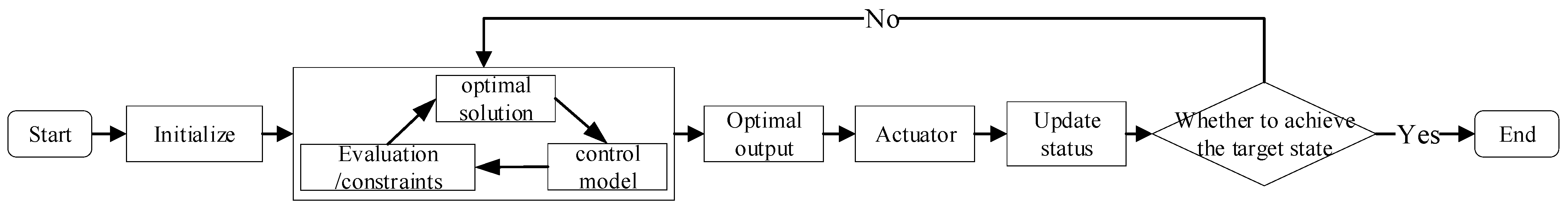
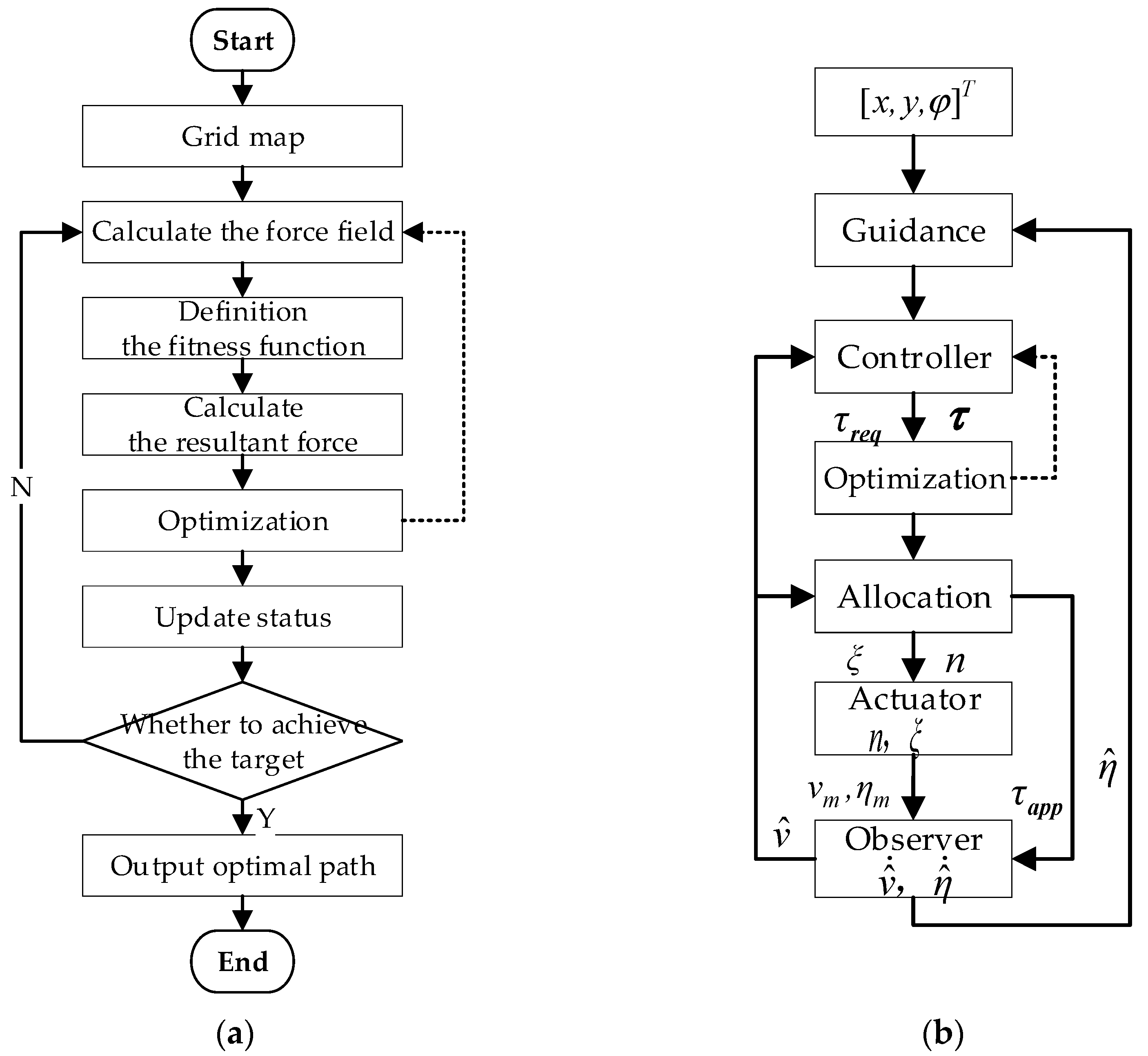
3.3. Autonomous Berthing Model of USV Based on CMA-ES

For ship motion control, in fact, it is difficult to accurately establish the ship mathematical model as it is a strong coupling nonlinear system. Fossen [34], Zhang [35] and other scholars have made some achievements in large ship motion control. As the ship usually navigates at a slow speed with a large drift angle when moving alongside the berth, there is a great difference from a ship sailing at normal speed. The current research concentrates primarily upon the minimization of path length and time expenditure. External environmental perturbations, physical constraints and restrictions to ship maneuvering are neglected although such factors would also exert great influence upon the ship handling characteristics of a vessel.

Aiming at the inadequacies of the algorithms employed in the current phase of ship control, the optimization of the berthing control system in this paper can primarily encompass two aspects: on the one hand, the constrained optimization of the ship’s navigation path is undertaken. According to the relevant navigation rules and constraints, a search and evaluation of all viable paths are performed and the optimal initialization path is selected, as delineated in Figure 3a. On the other hand, the optimization of the performance indices of the LQR controller is carried out, such as the optimization of the motion or amplitude stability indices.

As shown in Figure 3b, based on the CMA-ES algorithm, the objective function and constraints considering ship actuators like engine and steering gear for the optimizer are constructed and the improved LQR controller is given for the auto-berthing control problem.

The framework of the path planning algorithm selected for this work, the Artificial Potential Field (APF) method, is depicted in Figure 3a. The crux of the APF path planning method constitutes the construction of potential fields by computing the gravitation of the destination and the repulsion of obstacles, with the potential field gradient descent direction harnessed to instigate updates in movement. The process of CMA-ES optimization is to calculate whether the fitness function belongs to the threshold interval, otherwise, the weight is changed again to calculate the gravitation and repulsion. In the process of path planning using the APF algorithm [36], the resultant field is represented by $U(q)$, $U_{att}(q)$ is the gravitational field and $U_{rep}(q)$ is the repulsive field.

$$U(q)=U_{att}(q)+U_{rep}(q)$$

(19)

The framework schematic of the LQR control algorithm employed within this paper is delineated in Figure 3b. The optimizer CMA-ES calculates and finds the optimal value that meets the constraint conditions by adjusting the weight matrix parameters of state variables and control variables.

According to Formulas (2) and (11), Formula (20) is obtained, where the state matrix is $\mathit{A}({\nu }_r)=-{\mathit{M}}^{-1}(\mathit{C}({\nu }_r)+\mathit{D}({\nu }_r))$ and the control matrix is $\mathit{B}={\mathit{M}}^{-1}$.

$$\begin{array}{ll}\hfill {\dot{\nu }}_r& =\mathit{A}({\nu }_r){\nu }_r+\mathit{B}(\tau +{\tau }_{wind}+{\tau }_{current})\\ \hfill \dot{\eta }& =J_{\mathrm{\Theta }}(\eta ){\nu }_r+V_c\end{array}$$

(20)

According to the hydrodynamic model with large drift angle proposed by Yoshimura Yasuo, the ship model navigating at slow speed, especially when moving alongside the berth, is revised as (21), and the detailed derivation process and parameter explanation are shown in references [30,31]. The modified model is decomposed into (22) after being brought into the damping matrix D, where d is the original static constant, $\mathsf{\Phi }({\nu }_r)$ is a regression function and $\vartheta$ is an error parameter.

$$\{\begin{array}{l}{X}_{\mathrm{H}}=X_{\mathrm{H}}(r=0)+X_{\nu r}\nu r+X_{rr}{r}^2\\ Y_{\mathrm{H}}=Y_{\mathrm{H}}(r=0)+Y_r|u|r+\frac{1}{2}\rho d{C}_d\left(L\nu |\nu |-{\displaystyle {\int }_{-L/2}^{L/2}\left(\nu +C_{ry}xr\right)}|\nu +C_{ry}xr|\mathrm{d}x\right)\\ N_{\mathrm{H}}=N_{\mathrm{H}}(r=0)+N_r|u|r+\frac{1}{2}\rho d{C}_d{\displaystyle {\int }_{-L/2}^{L/2}\left(\nu +C_{rr}xr\right)}|\nu +C_{rn}xr|x\mathrm{d}x\end{array}$$

(21)

$$\begin{array}{ll}\hfill \mathit{D}({\nu }_r){\nu }_r& =-d{\nu }_r-\mathsf{\Phi }({\nu }_r)\vartheta :\\ \hfill d& =-diag([X_u,Y_{\nu },N_r])\\ \hfill \vartheta & ={[X_{\left|u\right|u},X_{uuu},Y_{\nu },Y_r,Y_{\left|\nu \right|\nu },Y_{\left|r\right|\nu },Y_{\left|\nu \right|r},Y_{\left|r\right|r},N_{\nu },N_{\left|\nu \right|\nu },N_{\left|r\right|\nu },N_{\left|\nu \right|r},N_{\left|r\right|r}]}^T\end{array}$$

(22)

Combining Equations (12) and (22), the control law, Equation (23), is obtained, where $R(\psi )$ is the rotation matrix about the Z axis.

$$\begin{array}{l}{\dot{\nu }}_r={\mathit{M}}^{-1}(\tau +{\tau }_{wind}+{\tau }_{current}-\mathit{C}({\nu }_r){\nu }_r+d{\nu }_r+\mathsf{\Phi }({\nu }_r)\vartheta )\\ \dot{\eta }=\mathit{R}(\psi ){\nu }_r+V_c\end{array}$$

(23)

$$\mathit{R}(\psi )=\left[\begin{array}{ccc}\cos \psi & -\sin \psi & 0\\ \sin \psi & \cos \psi & 0\\ 0& 0& 1\end{array}\right]$$

(24)

3.3.1. Constraint Condition

Basic state constraints (25) are to be satisfied when the ship berths, where $P_1={\left(x_1,y_1,{\psi }_1\right)}^T$ denotes the prescribed desired berthing state, $P1={\left(x1,y1,\psi 1\right)}^T$ is the motion state of the ship in actual motion control, $d\_ref$ and $\psi \_ref$ are the maximum allowable errors.

$$P1-P_1\le {[d\_ref,d\_ref,\psi \_ref]}^T$$

(25)

Position constraint is to reduce the optimized search space and stabilize the ship’s docking position more efficiently. The set berth area is ${Ⅱ}_C$ when the ship is within ${Ⅱ}_C$, and it is considered that the ship has entered the berth area. $p_i$ is the four points of the ship’s safety rectangle, and $C_{berth}$ represents the berth area.

As shown in Figure 4, The waters proximate to the berth are demarcated into three zones: Zone I (the outer stabilizing region beyond the berth), Zone II (the berth per se) and Zone III (the quayside wharf). The berthing process is likewise demarcated into three stages: Stage 1 (the approaching phase, arriving at the outer stabilizing region far from the berth), Stage 2 (outer stabilizing, adjusting the orientation of the ship’s head) and Stage 3 (berthing).

$${Ⅱ}_C={\displaystyle \sum }_{i=1}^4{{\displaystyle \int }}_{p_i\in C_{\mathrm{berth}}}\left|Y_i-Y_{\mathrm{berth}}\right|\mathrm{d}t$$

(26)

The control mechanism of a USV is composed of propellers and steering gear system and is limited by its own physical characteristics. This paper mainly considers the mechanical constraint $[C_{min},C_{max}]$ composed of rudder angle $\delta$ and propeller speed $n$ of the USV. The constraint $[C_{min}^{\prime },C_{max}^{\prime }]$ of rudder angle change rate ${\delta }^{\prime }$ and rotational speed change rate $n^{\prime }$ are also considered.

$$\begin{array}{c}{C}_{min}={[{\delta }_{\min },n_{\min }]}^T,C_{min}^{\prime }={[{\delta }_{\min }^{\prime },n_{\min }^{\prime }]}^T\\ C_{max}={[{\delta }_{\max },n_{\max }]}^T,C_{max}^{\prime }={[{\delta }_{\max }^{\prime },n_{\max }^{\prime }]}^T\end{array}$$

(27)

The ship berthing speed is restricted as per Equation (28), and $u_t$ and ${\nu }_t$ represent the longitudinal and lateral velocity of the ship at time $t$

$$\left|u_t\right|\le u_{\max },\left|{\nu }_t\right|\le {\nu }_{\max }$$

(28)

The constraint on the ship’s course is described in Equation (29), ${\psi }_t$ is the ship’s heading at time t and rot is the ship’s turn rate, that is, the course change rate.

$$\left|rot\right|=\left|\frac{\Delta \psi }{\Delta t}\ast \frac{180}{pi}\right|\le RO{T}_{\max }$$

(29)

3.3.2. Objective Function

The initial state of the system is defined as $x(0)$. The optimal control vector u* can be obtained by the LQR, and the state vector x at the next moment can be obtained by motion control of the ship. As the initial sample of the CMA-ES, the optimal state $x_i$ at the next moment can be obtained.

Suppose that the system state vector $x={(x,y,\psi )}^T$ and the control vector $\dot{u}={(n,\delta )}^T$, then Formula (23) is simplified to obtain the system state described in Equation (30), where the interference matrix $\mathit{H}={\mathit{M}}^{-1}({\tau }_{\mathrm{wind}}+{\tau }_{\mathrm{current}})$, $\mathit{f}(·)$ is the system state matrix.

$$\begin{array}{ll}\hfill \dot{x}& ={\mathit{M}}^{-1}(\mathit{d}x-\mathit{C}x)+{\mathit{M}}^{-1}(u+\mathsf{\Phi }\left(x\right)\vartheta )+{\mathit{M}}^{-1}({\tau }_{\mathrm{wind}}+{\tau }_{\mathrm{current}})\\ & =\mathit{f}\left(x\right)+{\mathit{M}}^{-1}\left(u+\mathsf{\Phi }\left(x\right)\vartheta \right)+\mathit{H}\\ \hfill y& =\mathit{R}(\psi )x+V_c\end{array}$$

(30)

The desired ideal output is set to ${\eta }^{*}(t)$ and $y(t)$ is the actual control output. $e(t)=y(t)-{\eta }^{*}(t)$ is the deviation, and the index functional of the control system is expressed as $J$.

$$J=\frac{1}{2}{e}^T(T)Se(T)+\frac{1}{2}{{\displaystyle \int }}_0^T\left(e^T(t)Q(t)e(t)+u^{\mathrm{T}}(t)R(t)u(t)\right)dt$$

(31)

In order to simplify the study of energy consumption of the ship power system, within this work, the control variables for the rudder and propellers during the ship berthing process are adopted as the energy consumption indices for the system. $n_t$ and ${\delta }_t$ are the sampling values at the corresponding time, ${\lambda }_1$ and ${\lambda }_2$ are the weight coefficients of the corresponding control variables. According to Formula (32), $F(n,\delta )$ [37] is calculated as the energy consumption index during the ship’s navigation.

$$F(n,\delta )={\displaystyle \sum }_{t=0}^{T-1}({\lambda }_1{n}_t^2+{\lambda }_2{\delta }_t^2)$$

(32)

The control objective function of the system can be written as Equation (33), where $K_J$ and $K_F$ are the corresponding weight parameters, the value is determined according to the actual situation and the value is [0.75, 0.25] in the experiment. Combined with Formula (19), the objective function of path planning is expressed as Equation (34), $H_U$ and $H_F$ are the corresponding weight functions and the values in the experiment are [0.25, 0.75].

$$K_J\ast J+K_F\ast F$$

(33)

$$H_U\ast U+H_F\ast F$$

(34)

In summary, the optimization objective function and constraint conditions of the berthing system can be described as Formulas (35) and (36).

$$\min \{\begin{array}{l}{H}_U\ast U+H_F\ast F\\ K_J\ast J(P,C)+K_F\ast F(n,\delta )\end{array}$$

(35)

$$s.t.\{\begin{array}{ll}\hfill P1-P_1& \le {[d\_ref,d\_ref,\psi \_ref]}^T\\ \hfill \left|u_t\right|& \le u_{\max }\\ \hfill \left|{\nu }_t\right|& \le {\nu }_{\max }\\ \hfill \left|rot\right|& \le RO{T}_{\max }\\ \hfill C_{\min }& \le C\le C_{\max }\\ \hfill C_{\min }^{\prime }& \le C^{\prime }\le C_{\max }^{\prime }\end{array}$$

(36)

Upon the actual berthing process, external environmental disturbance and the intrinsic physical maneuverability properties of the hull exert considerable influence on the behaviors of the vessel. In accordance with the actual hydrodynamic environments and maneuvering constraints inherent to the ship itself, corresponding constraints have been incorporated into the overall control process. An optimization strategy predicated upon the CMA-ES effects adaptive optimization of the safety and smoothness of the ship’s berthing trajectory as well as the outputs of the controller.

4. Simulation Analysis

The ship adopted in this experiment is a fully actuated ship, and the hydrodynamic coefficient of the model refers to the Otter ship model given by Fossen [31]. In this paper, two groups of simulation experiments are set up: group 1 implements automatic berthing of the vessel in external environments with no consideration of wind and current through employment of the LQR. The second group is the automatic berthing simulation experiment with consideration of wind and current environments by using the LQR and the integrated control system proposed in this paper.

No dynamic obstacles are set in the two sets of experiments in this paper. The configuration of the simulation environment of the experiment is shown in Table 2, the parameters of the simulated ship model used in the experiment are shown in

Table 3. Experimental environment.

Parameters	Configuration
System environment	Win11 Intel (R) Core (TM) i5-9500 CPU @3.00GHz 16G RAM

and the values of the relevant parameters of the experiment are shown in

Table 4. USV experimental ship model parameters.

Parameters	Value
Length (m)	2.00
Width B (m)	1.08
Draft (m)	0.1951
Mass m (kg)	55
Rotation radius (m)	0.432
Square coefficient	0.4
Rudder angle δ range (°)	[−35, 35]
Propeller speed n range (r/s)	[−50, 50]

and

Table 5. USV experimental simulation parameters.

Parameters	Value
Simulation map	100 m × 100 m
Initial point state	[90, 10, 120°]
Berthing point status	[7, 61, 0°]
$[u_{approah},u_{dock}]$	[3 m/s, 0.075 m/s]
$[d_{ref},{\psi }_{ref}]$	[0.01 m, 3°]
$[u_{\max },{\nu }_{\max }]$	[0.075 m/s, 0.075 m/s]
$RO{T}_{\max }$	2.5 °/s2
$[K_J,K_F,H_U,H_F]$	[0.75, 0.25, 0.25, 0.75]

.

4.1. Automatic Berthing of USV Based on LQR

In circumstances where the waters proximate to the berth do not show disturbances from a northerly or easterly wind or current, a static calm water condition is assumed, ${\mathit{\tau }}_{\mathrm{wind}}=[0,0]$, ${\mathit{\tau }}_{\mathrm{current}}=[0,0]$ (the unit is m/s). Granted the port berth articulates no particular stipulations regarding ship berthing, the testing shows that the vessel can be capable of directly affecting berthing. Through experimental simulation, the berthing process is delineated in Figure 5.

For the secondary berthing phase depicted in Figure 5b, with the ship stabilized outside of the berth, the lateral berthing maneuver is executed based on distance detection data from shipborne sensors indicating proximity to the berth terminal. In this process, the ship’s posture must adjust flexibly according to the optimal control outputs generated by the LQR controller to facilitate lateral berthing of the ship and, ultimately, automatic berthing is completed.

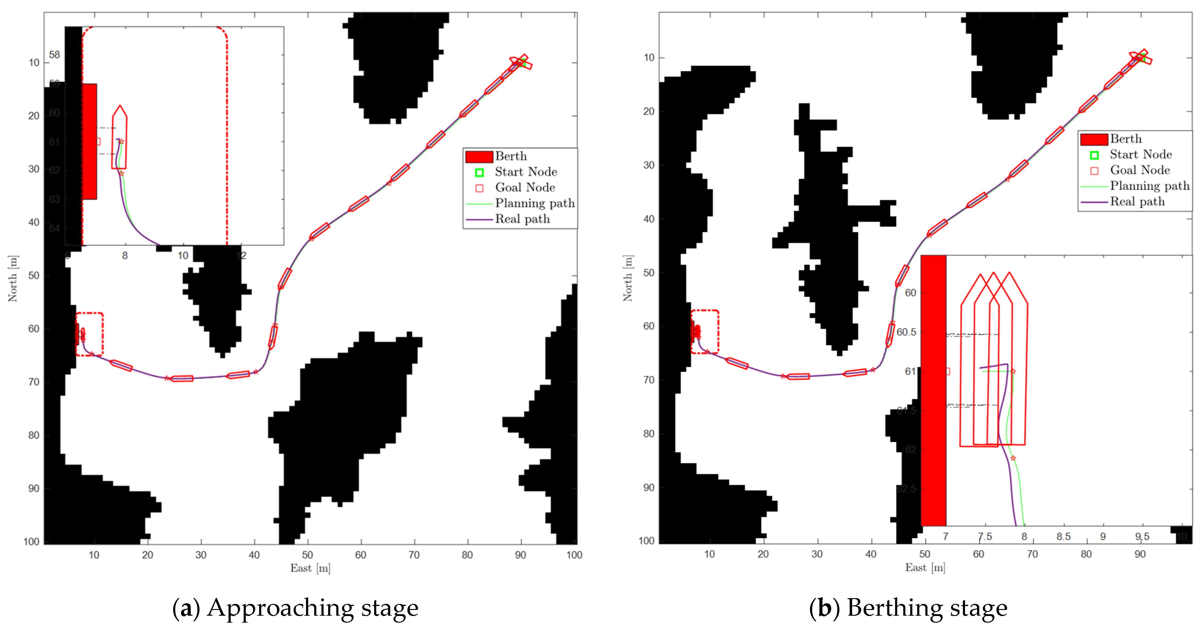
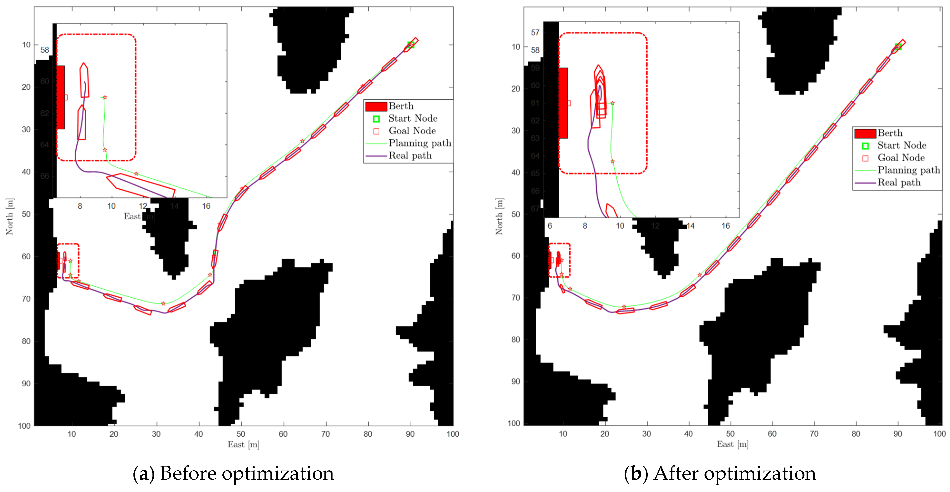
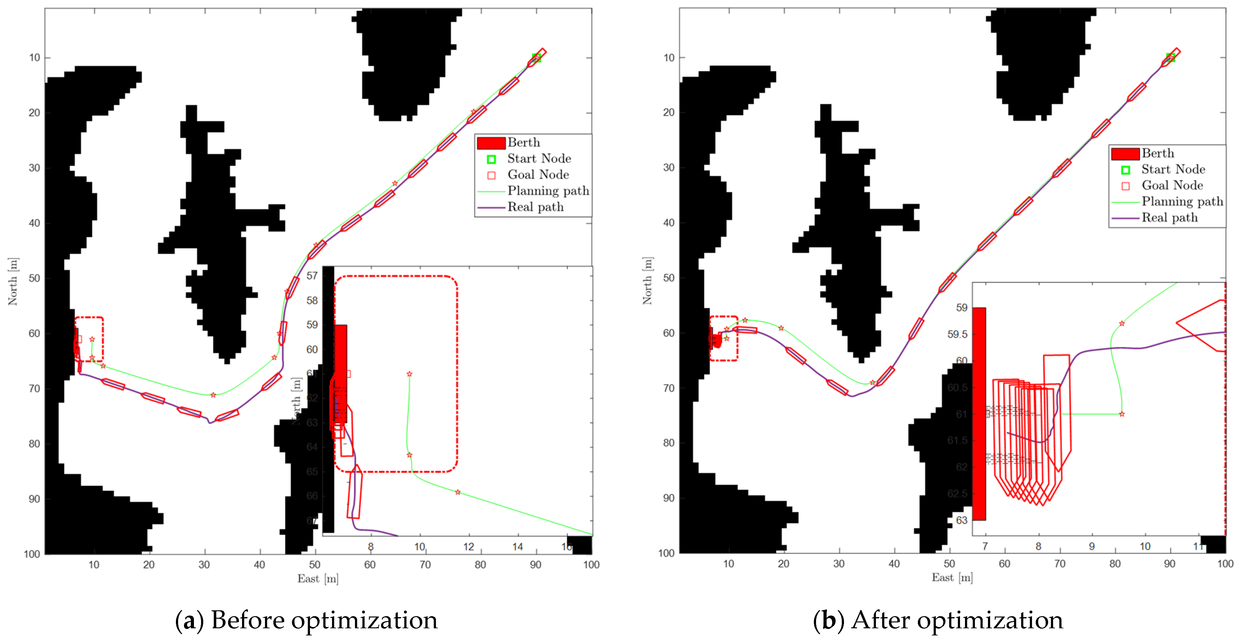
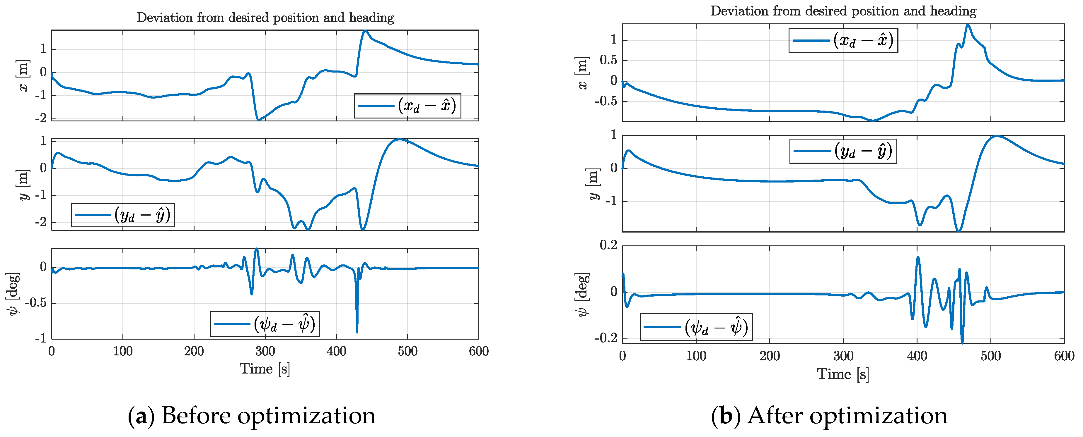
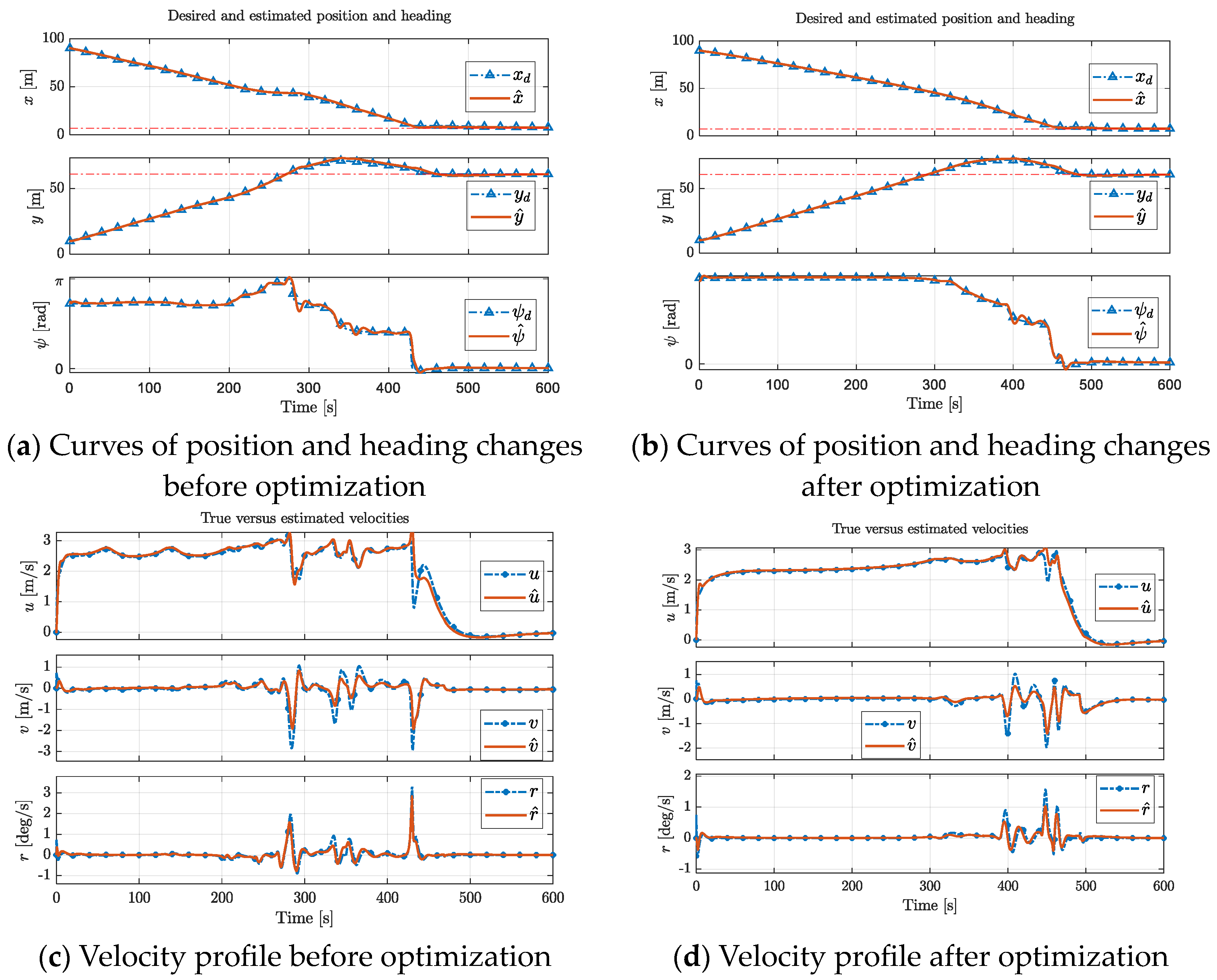
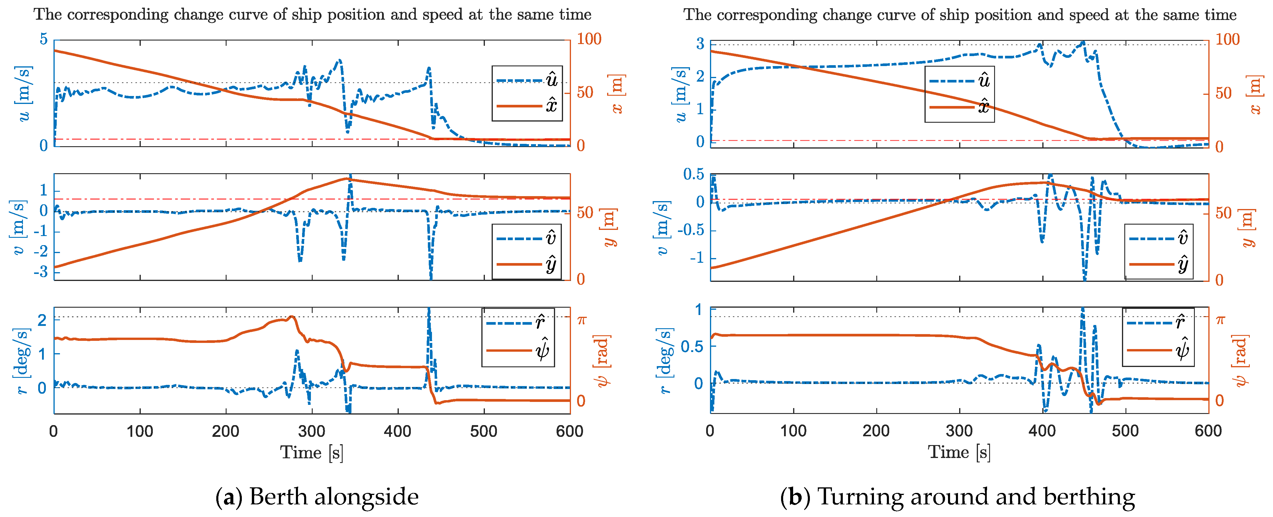
4.2. Automatic Berthing of USV Based on CMA-ES Optimization

The USV approaches the berth with perturbations from northerly and easterly winds and currents, ${\mathit{\tau }}_{\mathrm{wind}}=[1.5,-2.5]$, ${\mathit{\tau }}_{\mathrm{current}}=[-0.2572,-0.0514]$ (the unit is m/s). Compared with the ideal environment of group 1, group 2 considers the environmental perturbations from wind and current, which shows effective validation of the algorithm’s robustness under simulation conditions and they are also much closer to the real situation during ship berthing.

In accordance with the framework of the auto-berthing control system shown in Figure 3, during the path planning phase the CMA-ES algorithm optimizes the APF berthing path planning, rendering the ship’s motion path safer and smoother. By fully considering the maneuvering constraints intrinsic to the ship itself and the frequency and amplitude of changes in the ship’s rotational velocity and rudder angle, all those constraints ensure the actual ship motion dynamics are as close as possible to the real berthing process. In Figure 6, the simulation results with CMA-ES optimization at the initial berthing stage are illustrated.

For the second berthing stage illustrated in Figure 7, motion constraints imposed on the ship’s steering gear and propeller aim to exclude high-frequency control inputs to the steering gear during the berthing process. The performance metrics of the controller are optimized via the CMA-ES method, enabling its rapid and stable convergence to the desired state and completing the berthing task.

Ships get as close to the berth against the wind and current as possible in tidal harbors of China, as mentioned in reference [38]. In actual berthing operations, choosing a strategy of berthing against the wind and current can prevent the ship from being pushed away by the current and wind. The experimental water area is subject to wind and current interference in the north and east directions (${\mathit{\tau }}_{\mathrm{wind}}=[2,-3.5]$,${\mathit{\tau }}_{\mathrm{current}}=[-1.0289,0.514]$, the unit is m/s), as shown in Figure 8.

Hence, Figure 8a delineates the outcome of the berthing methodology being adopted under the identical experimental conditions. Owing to the substantial current, the drifting motion of the vessel is rather conspicuous. A considerably large inertial residual velocity is still maintained adjacent to the berth, which poses a grave peril to the execution of the vessel’s berthing operation. By executing a turning maneuver, the collision risk imposed by the drifting motion when the vessel comes to a stop adjacent to the berth is averted, as shown in Figure 8b.

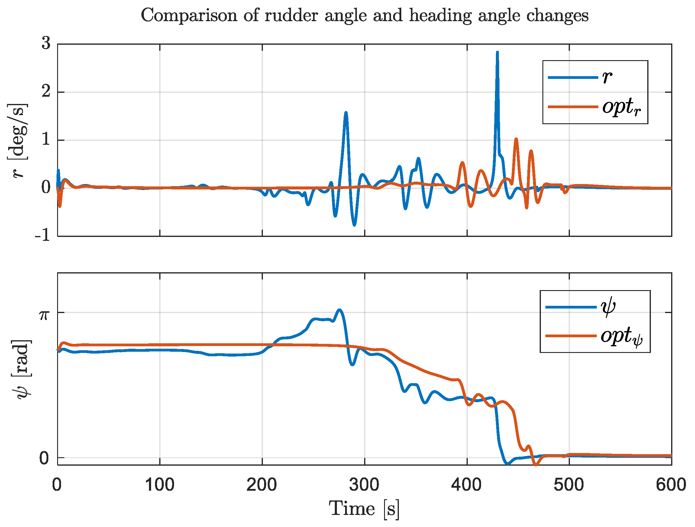
4.3. Result Analysis

By comparing Figure 5, Figure 6 and Figure 7, it is shown that the wind and current have a great influence on the ship’s motion. From the berthing stages in Figure 5b and Figure 7a, we can find the influence of wind and current on the ship’s low-speed motion: the wind interference will cause ships, especially small ships, to deviate greatly from the planned trajectory at low speed.

Figure 6 and Figure 7 delineate the autonomous berthing process of a USV under specific wind and current interference conditions (stabilization outside the berth followed by parallel berthing). Figure 6a and Figure 7a represent the nonoptimized scenarios. Figure 6b and Figure 7b display the optimal control profiles obtained through the CMA-ES optimization approach. A comparative analysis between Figure 7a,b reveals that even with wind and current, the CMA-ES optimized control system still shows competence in mitigating abrupt fluctuations in the ship’s motion and amplitude.

Specifically, in the berthing path planning in Figure 6, the left side of Figure 6a is without optimization processing. In the middle part of the figure, the path planned by the APF algorithm has many waypoints. After optimization processing, Figure 6b has much less twisting and turning, and the overall path becomes smoother. This smoothed path can effectively reduce the rudder angle changes of the ship during sailing and reduce the number of manipulations, and this change can be verified in the curve of the ship’s rudder angle changes in Figure 9.

The enlarged part of Figure 7 shows the final berthing process of the ship. The left figure shows the result of LQR control without optimization, and the right figure shows the result after optimization. Comparison shows that the process shown in the optimized Figure 7b is more acceptable. From the evaluation of the berthing effect, the berthing error after optimization is better, and the error curve in Figure 10 can support this result.

Through the comparison of the optimization of the whole control process in Figure 6 and Figure 7, it is found that the optimized effect of the CMA-ES is significant.

A comparison between Figure 9a,b demonstrates that the incorporation of path optimization significantly alleviates the abrupt changes in the ship’s heading during navigation. Within the simulation time span of 0 to 400 s, the optimized path results in smoother motion. During the 400 to 600 s period when the ship proceeds to the second docking stage, the path optimization enables the ship to make minimal attitude adjustments to satisfy the target state with smoother changes in heading angle and position, eliminating any instantaneous mutations. Meanwhile, it can be observed that the optimized path is more amenable as the input for the controller, yielding higher consistency between the actual ship motion and the planned path.

A comparison between Figure 9c,d indicates that the path optimization augments the fault tolerance of the ship’s output control during the first docking stage. The speed profile in Figure 9c exhibits frequent fluctuations with evident instantaneous reversals in polarity, which are undoubtedly deleterious to the ship’s steering control. In contrast, Figure 9d does not show such issues. Meanwhile, it can be observed that incorporating the optimization function in the second docking stage renders the output of the LQR controller more stable. Compared to the sharp increases and decreases in Figure 9c, the curve in Figure 9d demonstrates that the overall process does not incur rapid changes in either speed or rudder angle, cohering with the actual operation of ship berthing maneuvers.

Obviously, it can also be found from Figure 9c,d that even if the frequency and amplitude of the rudder angle change are reduced as a whole, the optimized rudder angle is more frequent than before in the docking stage during the 400 to 600 s, which may be caused by the high accuracy setting.

In contrast, the control system optimized by the CMA-ES demonstrates higher accuracy in control effect and greater energy saving of the system, as evidenced by the heading variation frequency and amplitude illustrated in Figure 10.

According to the simulation results of the two berthing strategies under the same environment in Figure 8, it can be analyzed that: when there are strong wind and current disturbances to the ship’s berthing motion, the control difficulty of the ship increases in Figure 8a when berthing directly, and the probability of collision with the berth is increased; the turning strategy in Figure 8b can effectively offset the strong wind and current interference to the ship and ensure the safety of ship berthing. Choosing a suitable berthing strategy is also a way to reduce the risk of berthing collision and ensure the safety of ship berthing. The motion process curves of the two different berthing strategies are shown in Figure 11.

Analysis of Figure 12 indicates that the optimized rudder angle profile displays significantly reduced fluctuations with lower magnitude of changes; the abrupt shifts in heading angle have been eliminated, resulting in a smoother curve. By comparing the simulation results of the two berthing strategies, the optimized path (we understand it as strategy 2, that is, turning around is required under the current environment) appears generally smoother, decreasing the frequency of steering gear operation during ship berthing. Within the experimental setting of this study and given the berthing maneuver strategy employed, it warrants attention that the conditions should entail a relatively stable state of wind and current; more substantial marine environmental interferences can compromise the stability of the ship’s autonomous berthing process.

5. Conclusions

In this paper, a complete framework of a berthing control system is proposed, and the berthing control system based on an LQR controller is optimized by the CMA-ES. During the experiment, the dynamic factors of the ship, the interference of the natural environment and the energy consumption of motion are fully considered. The results show that the berthing process of the ship can be well controlled, which is in line with the experimental expectation. The simulation results show that the automatic berthing system based on the CMA-ES proposed in this paper is feasible. However, in the current experimental process, there are still some shortcomings, such as the shallow water bank effect of the ship not being considered and the gain parameters of the controller cannot fully adapt to the model changes. In the future, we will continue to carry out in-depth research on the autonomous berthing of USVs and complete the algorithm test in a real environment in combination with a real testing ship.

References

1. Kose, K.; Fukudo, J.; Sugano, K.; Akagi, S.; Harada, M. Study on a Computer Aided Manoeuvring System in Harbours. Nav. Archit. Ocean. Eng. 1987, 25, 105–113. [Google Scholar]
2. Mizuno, N.; Uchida, Y.; Okazaki, T. Quasi Real-Time Optimal Control Scheme for Automatic Berthing. IFAC Pap. Line 2015, 48, 305–312. [Google Scholar] [CrossRef]
3. Zhang, Q.; Zhang, X.; Im, N. Ship nonlinear-feedback course keeping algorithm based on MMG model driven by bipolar sigmoid function for berthing. Int. J. Nav. Archit. Ocean. Eng. 2017, 9, 525–536. [Google Scholar] [CrossRef]
4. Xu, H.X.; Zhu, M.F.; Yu, W.Z. Robust adaptive control for automatic berthing of intelligent ships. J. Huazhong Univ. Sci. Technol. (Nat. Sci. Ed.) 2020, 48, 25–29. [Google Scholar]
5. Han, Z.Z. Simulation Study on Automatic Berthing of Ships Based on Active Disturbance Rejection Neural Network Control. Master’s thesis, Dalian Maritime University, Dalian, China, 2020. [Google Scholar]
6. Jia, Y.P.; Shen, H.L.; Yin, Y.; Zhang, X.F. Simulation of autonomous berthing of unmanned ships based on neural network. China Navig. 2021, 44, 107–111. [Google Scholar]
7. Wang, S.; Jin, H.; Meng, L.; Li, C. Optimize motion energy of AUV based on LQR control strategy. In Proceedings of the 2016 35th Chinese Control Conference (CCC), Chengdu, China, 27–29 July 2016; IEEE: Piscataway, NJ, USA, 2016; pp. 4615–4620. [Google Scholar]
8. Yang, S.F. Research on Multi-Objective Optimization Based on Adaptive Learning Mechanism of Covariance Matrix. Master’s thesis, Guizhou University, Guiyang, China, 2019. [Google Scholar]
9. Maki, A.; Sakamoto, N.; Akimoto, Y.; Nishikawa, H.; Umeda, N. Application of optimal control theory based on the evolution strategy (CMA-ES) to automatic berthing. J. Mar. Sci. Technol. 2020, 25, 221–233. [Google Scholar] [CrossRef]
10. Maniyappan, S.; Umeda, N.; Maki, A.; Akimoto, Y. Effectiveness and mechanism of broaching-to prevention using global optimal control with evolution strategy (CMA-ES). J. Mar. Sci. Technol. 2021, 26, 382–394. [Google Scholar] [CrossRef]
11. Miyauchi, Y.; Maki, A.; Umeda, N.; Rachman, D.M.; Akimoto, Y. System parameter exploration of ship maneuvering model for automatic docking/berthing using CMA-ES. J. Mar. Sci. Technol. 2022, 27, 1065–1083. [Google Scholar] [CrossRef]
12. Yazdanpanah, R.; Mahjoob, M.J.; Abbasi, E. Fuzzy LQR controller for heading control of an unmanned surface vessel. In Proceedings of the International Conference in Electrical and Electronics Engineering, Selangor, Malaysia, 4–5 December 2013; pp. 73–78. [Google Scholar]
13. Brasel, M. Adatpive LQR control system for the nonlinear 4-DoF model of a container vessel. In Proceedings of the 2013 18th International Conference on Methods & Models in Automation & Robotics (MMAR), Miedzyzdroje, Poland, 26–29 August 2013; IEEE: Piscataway, NJ, USA, 2013; pp. 711–716. [Google Scholar]
14. Shao, C. Research on Large Ship Maneuvering Motion Control Based on LQR. Master’s thesis, Shanghai Jiao Tong University, Shanghai, China, 2017. [Google Scholar]
15. Esmailian, E.; Farzanegan, B.; Malekizadeh, H.; Ghassemi, H.; Ardestani, M.F.; Menhaj, M.B. Control System Design for a Surface Effect Ship by Linear-Quadratic Regulator Method. J. Mar. Eng. 2017, 13, 47–56. [Google Scholar]
16. Tian, T. Research on Rudder Roll Stabilization Control System Based on Robust Optimal Control. Master’s thesis, Harbin Engineering University, Harbin, China, 2021. [Google Scholar]
17. Zhao, Y.; Zhang, Z.; Wang, J.; Wang, H. Fin-Rudder Joint Control Based on Improved Linear-Quadratic-Regulator Algorithm. IEEE Access 2022, 10, 111105–111114. [Google Scholar] [CrossRef]
18. Chen, J.Y. Walking Optimization of Simulated Soccer Robot Based on Improved CMA-ES. Master’s thesis, Nanjing University of Posts and Telecommunications, Nanjing, China, 2020. [Google Scholar]
19. Maki, A.; Sakamoto, N.; Akimoto, Y.; Banno, Y.; Maniyappan, S.; Umeda, N. On broaching-to prevention using optimal control theory with evolution strategy (CMA-ES). J. Mar. Sci. Technol. 2021, 26, 71–87. [Google Scholar] [CrossRef]
20. Maki, A.; Akimoto, Y.; Naoya, U. Application of optimal control theory based on the evolution strategy (CMA-ES) to automatic berthing (part: 2). J. Mar. Sci. Technol. 2021, 26, 835–845. [Google Scholar] [CrossRef]
21. Liu, Z.L.; Yuan, S.Z.; Zheng, L.H.; Jiang, J.Y.; Sun, Y.X. The development status and trend of ship automatic berthing technology. China Shipbuild. 2021, 62, 293–304. [Google Scholar]
22. Akimoto, Y.; Miyauchi, Y.; Maki, A. Saddle Point Optimization with Approximate Minimization Oracle and Its Application to Robust Berthing Control. ACM Trans. Evol. Learn. Optim. 2022, 2, 1–32. [Google Scholar] [CrossRef]
23. Miyauchi, Y.; Sawada, R.; Akimoto, Y.; Umeda, N.; Maki, A. Optimization on planning of trajectory and control of autonomous berthing and unberthing for the realistic port geometry. Ocean. Eng. 2022, 245, 110390. [Google Scholar] [CrossRef]
24. Homburger, H.; Wirtensohn, S.; Reuter, J. Docking control of a fully-actuated autonomous vessel using model predictive path integral control. In Proceedings of the 2022 European Control Conference (ECC), London, UK, 12–15 July 2022; IEEE: Piscataway, NJ, USA, 2022; pp. 755–760. [Google Scholar]
25. Sawada, R.; Hirata, K.; Kitagawa, Y.; Saito, E.; Ueno, M.; Tanizawa, K.; Fukuto, J. Path following algorithm application to automatic berthing control. J. Mar. Sci. Technol. 2021, 26, 541–554. [Google Scholar] [CrossRef]
26. Zhang, H.; Yin, C.; Zhang, Y.; Jin, S.; Li, Z. Reinforcement Learning from Demonstrations by Novel Interactive Expert and Application to Automatic Berthing Control Systems for Unmanned Surface Vessel. arXiv 2022, arXiv:2202.113252022. [Google Scholar]
27. Kamil, A.; Melhaoui, Y.; Mansouri, K.; Rachik, M. Artificial neural network and mathematical modeling of automatic ship berthing. Commun. Math. Biol. Neurosci. 2022, 2022, 113. [Google Scholar]
28. Xu, Z.; Galeazzi, R. Guidance and Motion Control for Automated Berthing of Twin-waterjet Propelled Vessels. IFAC-Pap. Line 2022, 55, 58–63. [Google Scholar] [CrossRef]
29. China Classification Society. Guidelines for Autonomous Cargo Ships (2018) Released. Ship Stand. Eng. 2018, 51, 53. [Google Scholar]
30. Yoshimura, Y. Study on Mathematical Model of Steering Motion in Shallow Water (Part 2): Fluid Forces Acting on Main Hull during Low-speed Steering. J. Kansai Shipbuild. Ocean. Eng. 1988, 77–84. [Google Scholar]
31. Fossen, T.I. Handbook of Marine Craft Hydrodynamics and Motion Control; John Wiley & Sons: Hoboken, NJ, USA, 2011. [Google Scholar]
32. Sun, B.D. Theoretical Basis of Modern Control, 4rd ed; Mechanical Industry Press: Beijing, China, 2018. [Google Scholar]
33. Hansen, N.; Kern, S. Evaluating the CMA evolution strategy on multimodal test functions. In Proceedings of the PPSN 2004: Parallel Problem Solving from Nature—PPSN VIII, Birmingham, UK, 18–22 September 2004; Springer: Berlin/Heidelberg, Germany, 2004; Volume 8, pp. 282–291. [Google Scholar]
34. Fossen, T.I. A nonlinear unified state-space model for ship maneuvering and control in a seaway. Int. J. Bifurc. Chaos 2005, 15, 2717–2746. [Google Scholar] [CrossRef]
35. Zhang, X.K.; Zhang, G.Q. Simple and Robust Control of Ship Maneuvering in Port. China Navig. 2014, 37, 31–34. [Google Scholar]
36. Khatib, O. Real-Time Obstacle Avoidance for Manipulators and Mobile Robots. Int. J. Robot. Res. 1986, 5, 90–98. [Google Scholar] [CrossRef]
37. Liu, X.Z. Research on Automatic Berthing Control of Ships Based on Optimal Trajectory Planning. Master’s thesis, Dalian Maritime University, Dalian, China, 2020. [Google Scholar]
38. Fu, Z.-Y. Self-reliant berthing and unberthing operation of small and medium-sized ships in restricted waters of tidal ports. China. Water Transport. (First Half Mon.) 2019, 56–58. [Google Scholar] [CrossRef]
Figure 1. Architecture of ship autonomous berthing system.
Jmse 11 01400 g001
Figure 2. A schematic of USV’s three degrees of freedom.
Jmse 11 01400 g002
Figure 3. System control optimization strategy. (a) Path planning; (b) LQR controller.
Jmse 11 01400 g003
Figure 4. Berthing area.
Jmse 11 01400 g004
Figure 5. USV auto-berthing process based on LQR without wind or current. (Black indicates the non-navigable area of the map, and the red dashed line indicates the berth area Ⅰ mentioned in Figure 4, the same as below.)
Jmse 11 01400 g005
Figure 6. The approaching process before and after optimization with wind and current.
Jmse 11 01400 g006
Figure 7. The auto-berthing process before and after optimization with wind and current.
Jmse 11 01400 g007
Figure 8. Two berthing methods with wind and current.
Jmse 11 01400 g008
Figure 9. Comparison of motion parameters in the approaching stage. (The red represents the actual, and the blue curve is the predicted.)
Jmse 11 01400 g009
Figure 10. Location and heading error values.
Jmse 11 01400 g010
Figure 11. Comparison of motion process parameters of different berthing strategies. (The blue dotted line on the left axis represents the speed change curve of the movement, and the red solid line on the right axis represents the position change curve.)
Jmse 11 01400 g011
Figure 12. Changes in ship heading and heading angle before and after optimization.
Jmse 11 01400 g012