
Quantifying Mechanisms Responsible for Extreme Coastal Water Levels and Flooding during Severe Tropical Cyclone Harold in Tonga, Southwest Pacific

 , , ,
, , ,  , and
, and
Abstract
1. Introduction
2. Method and Data
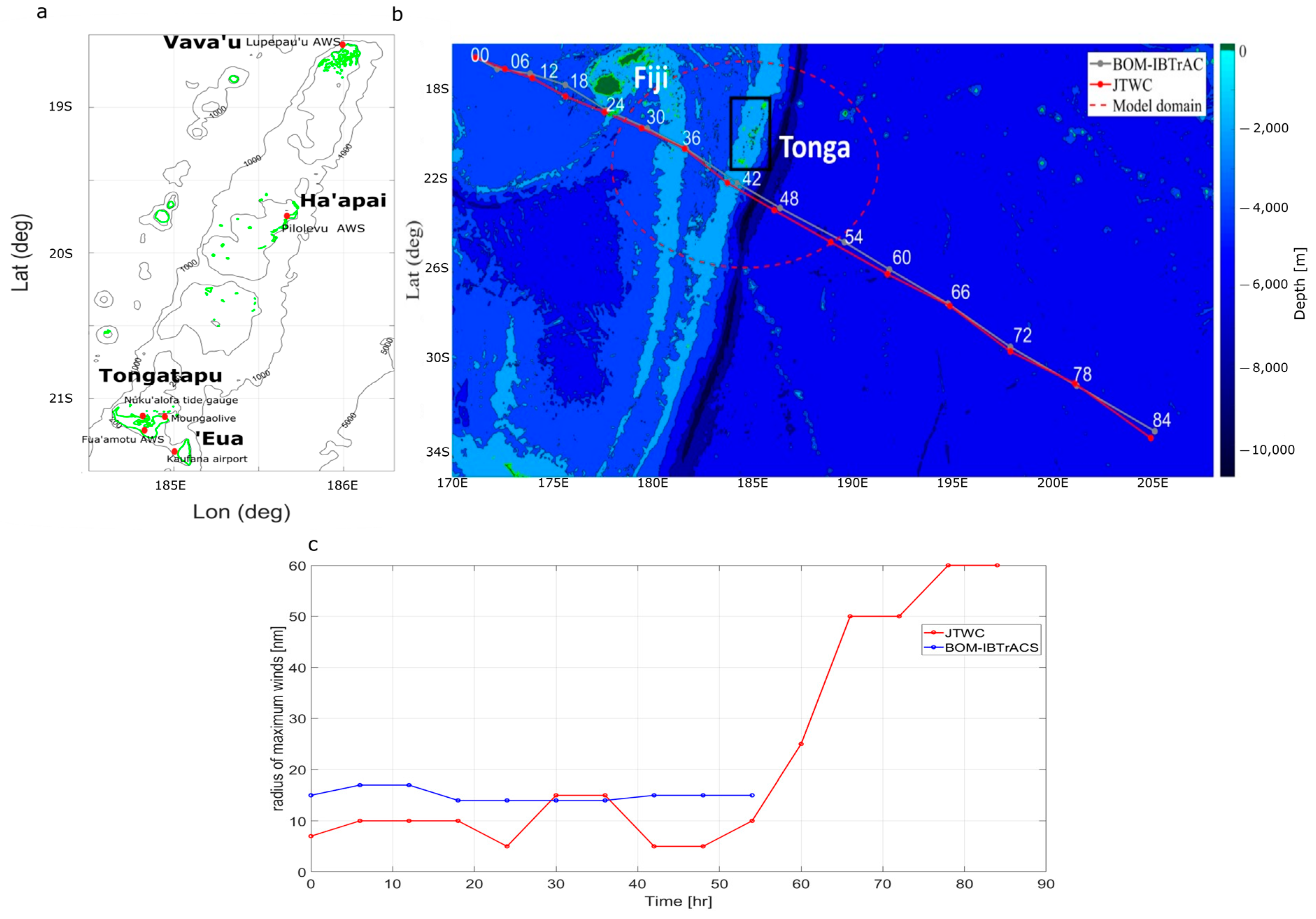
2.1. Study Site
2.2. Met-Ocean Measurements
2.3. TC Track Data
2.4. Atmospheric Forcing—Dynamic Holland Model
2.5. Model Setup
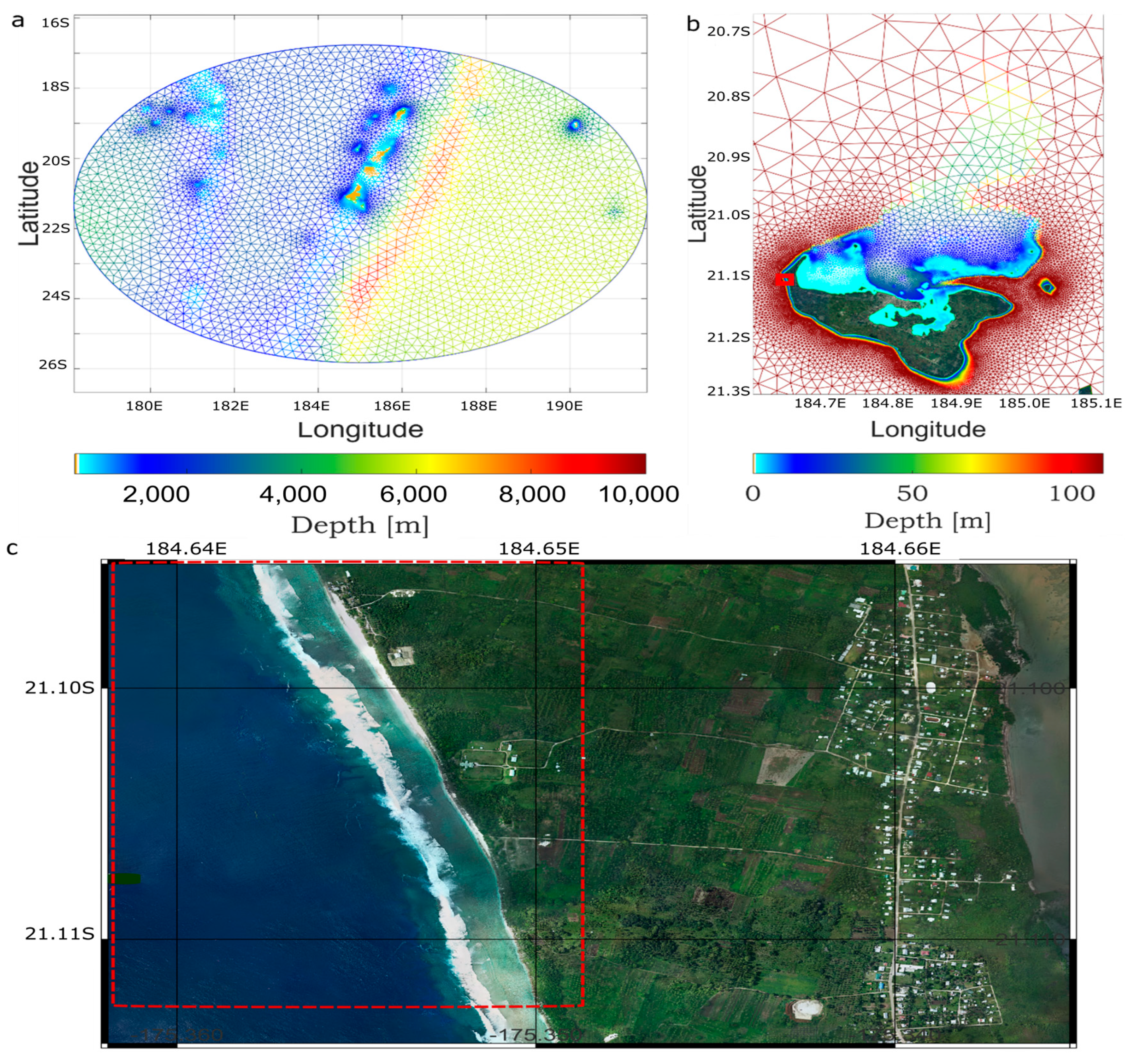
2.5.1. ADCIRC and SWAN Model Domain
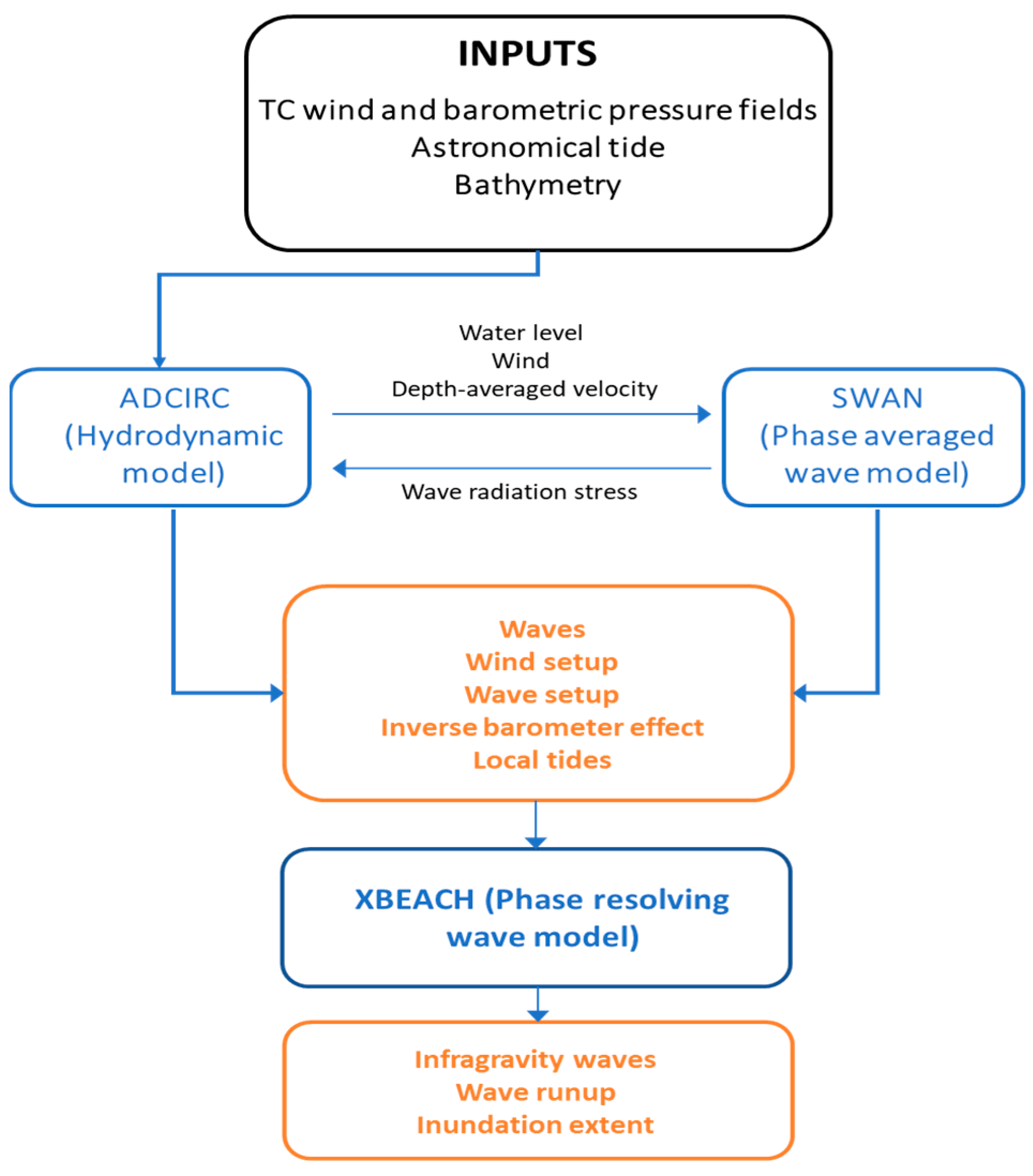
2.5.2. ADCIRC and SWAN Models
2.5.3. XBEACH
2.6. Experiment Design
3. Results and Discussions
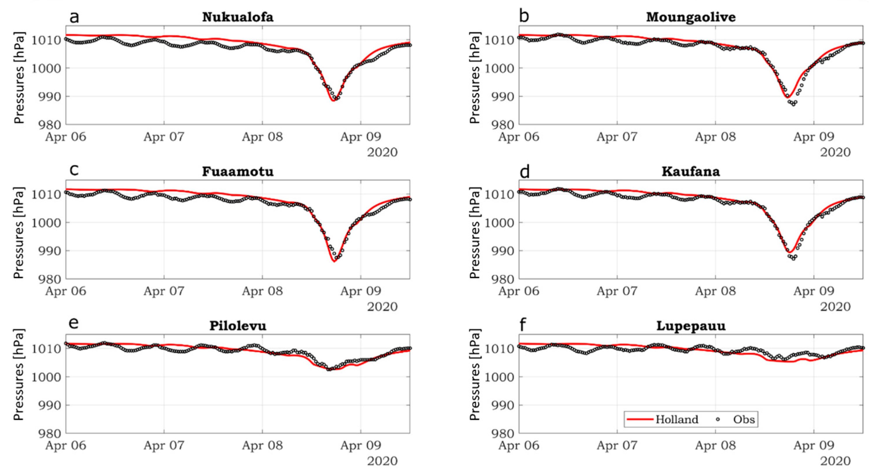
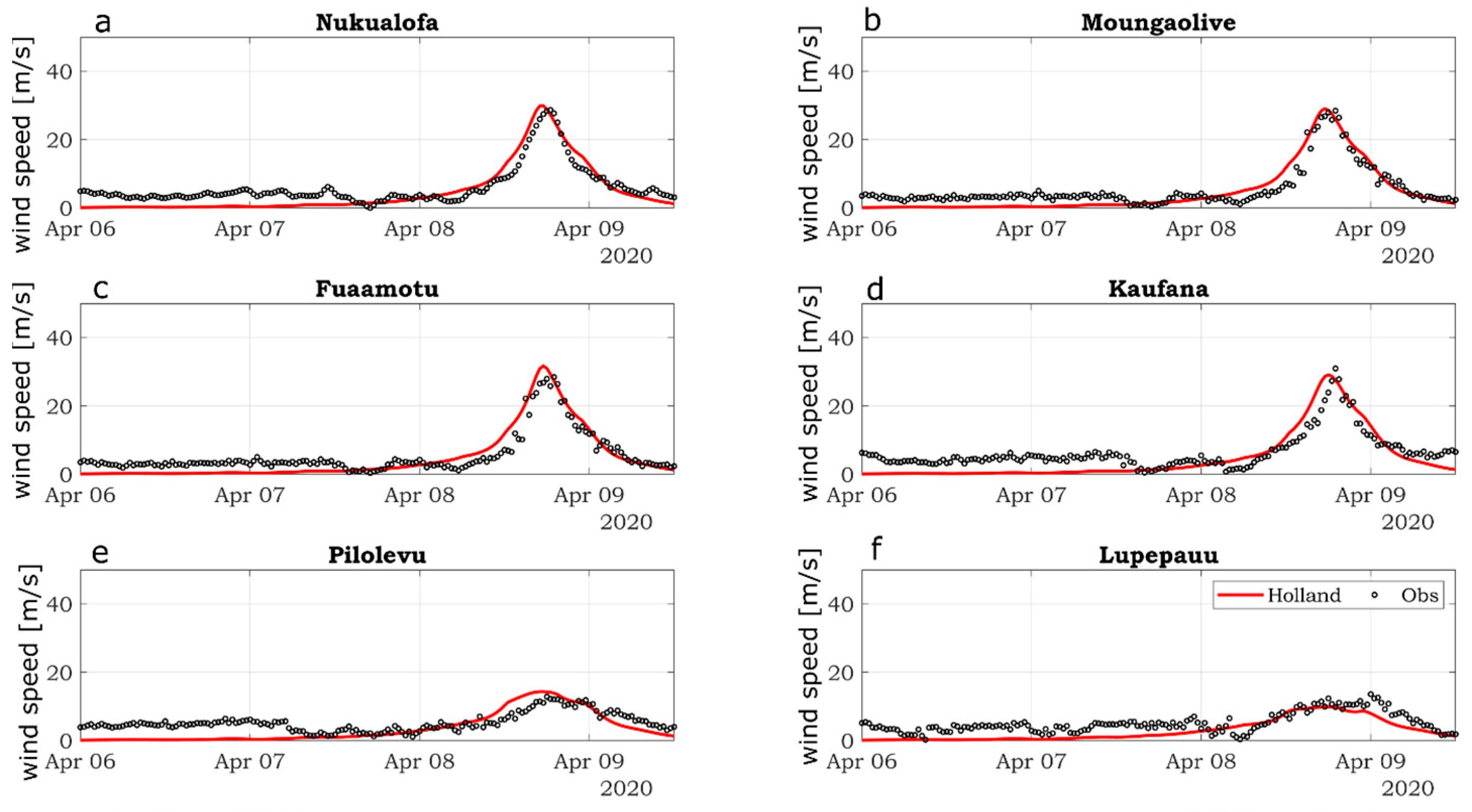
3.1. Validating the Dynamic Holland Model Performance
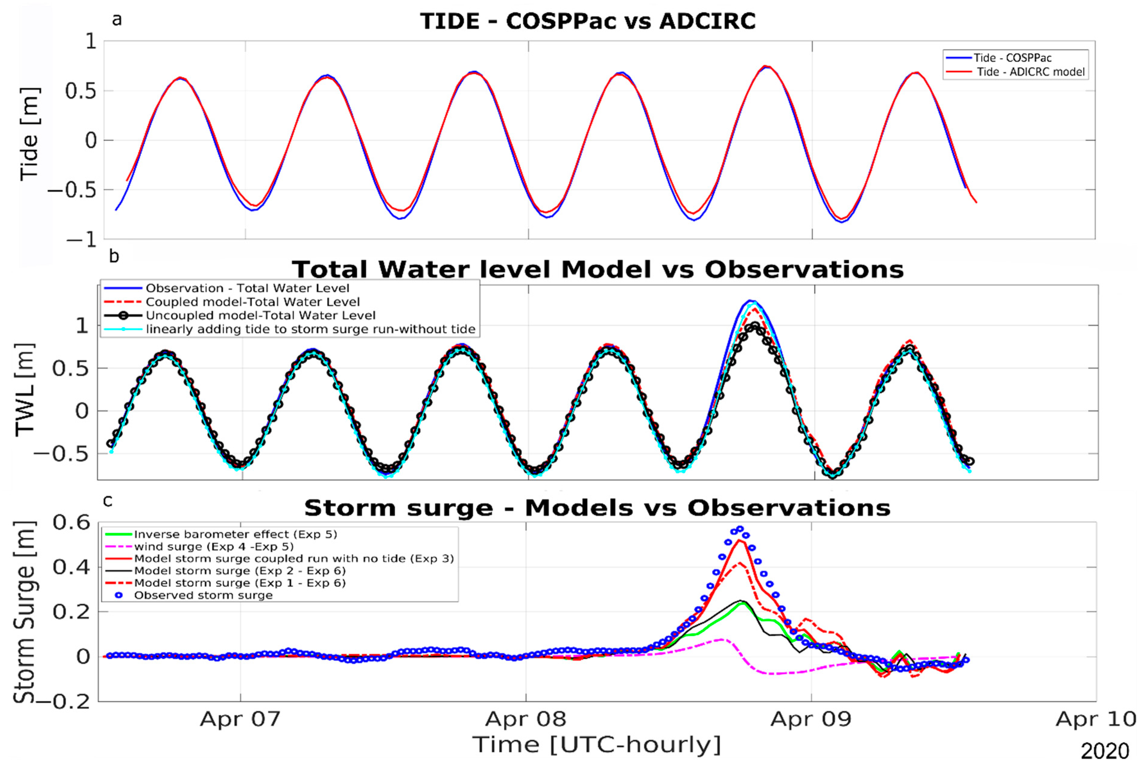
3.2. Astronomical Tide
3.3. Total Water Level (TWL) and Storm Surge Validation
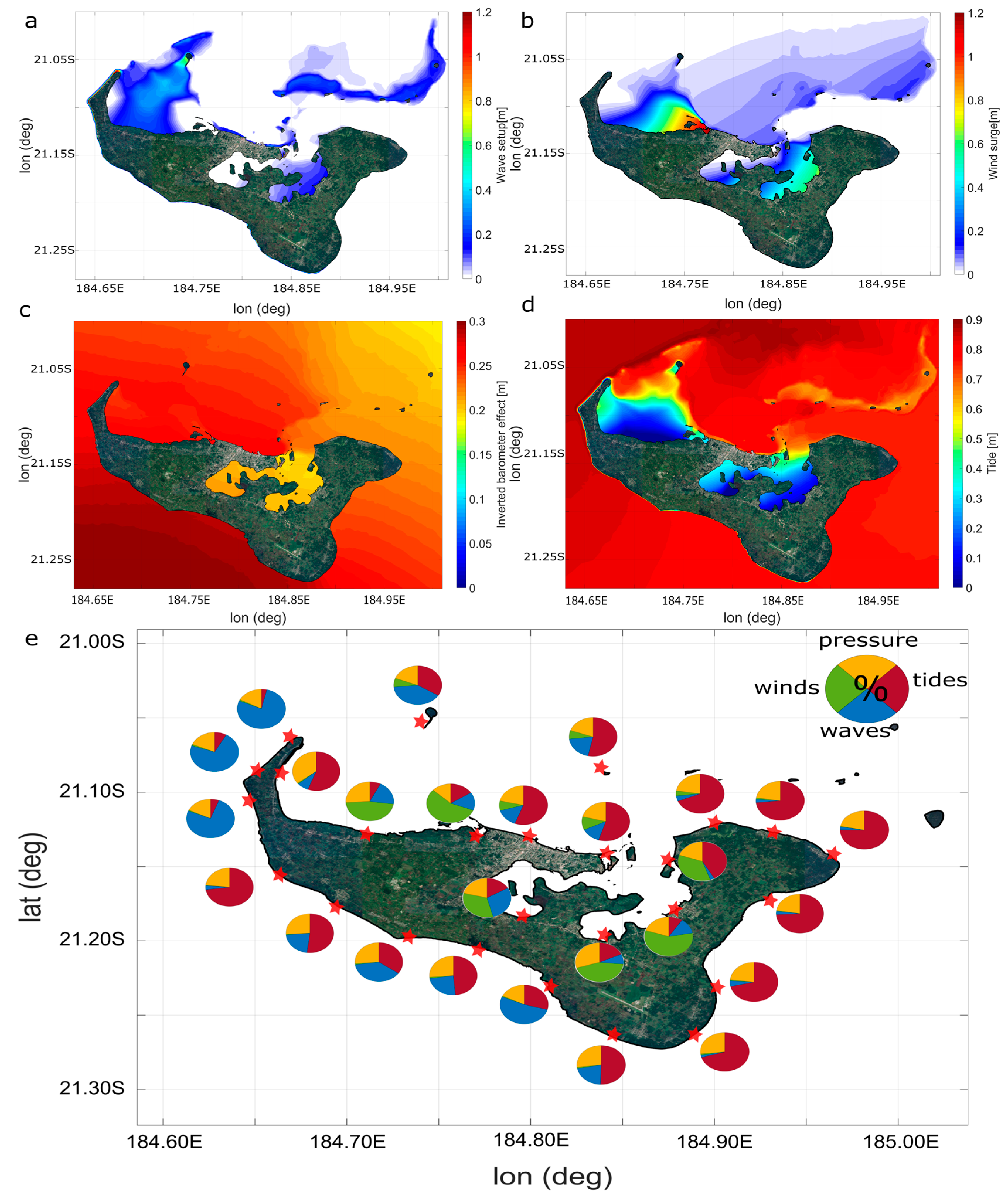
3.4. Relative Contributions of Different Forcings to the Total Water Levels
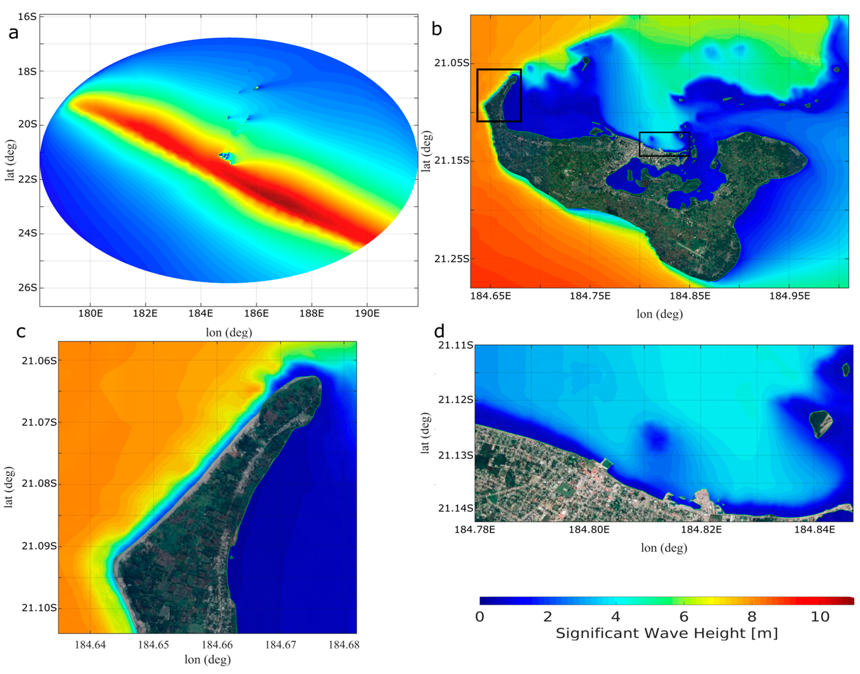
3.4.1. Wave Setup
3.4.2. Wind Setup
3.4.3. Atmospheric Pressures
3.4.4. Tides
3.5. Storm Surge—With and without Tides
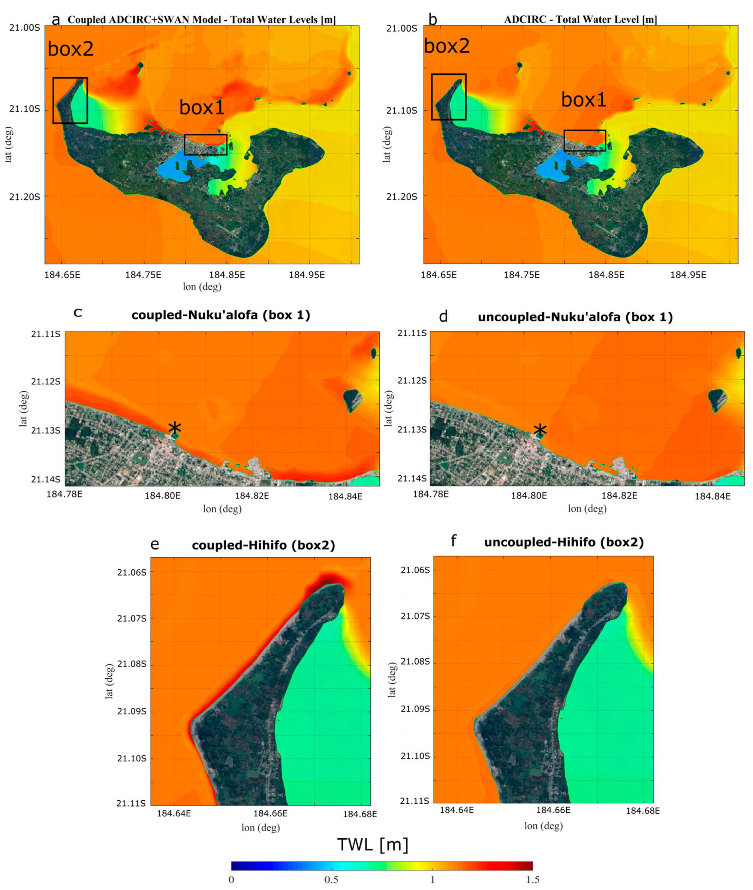
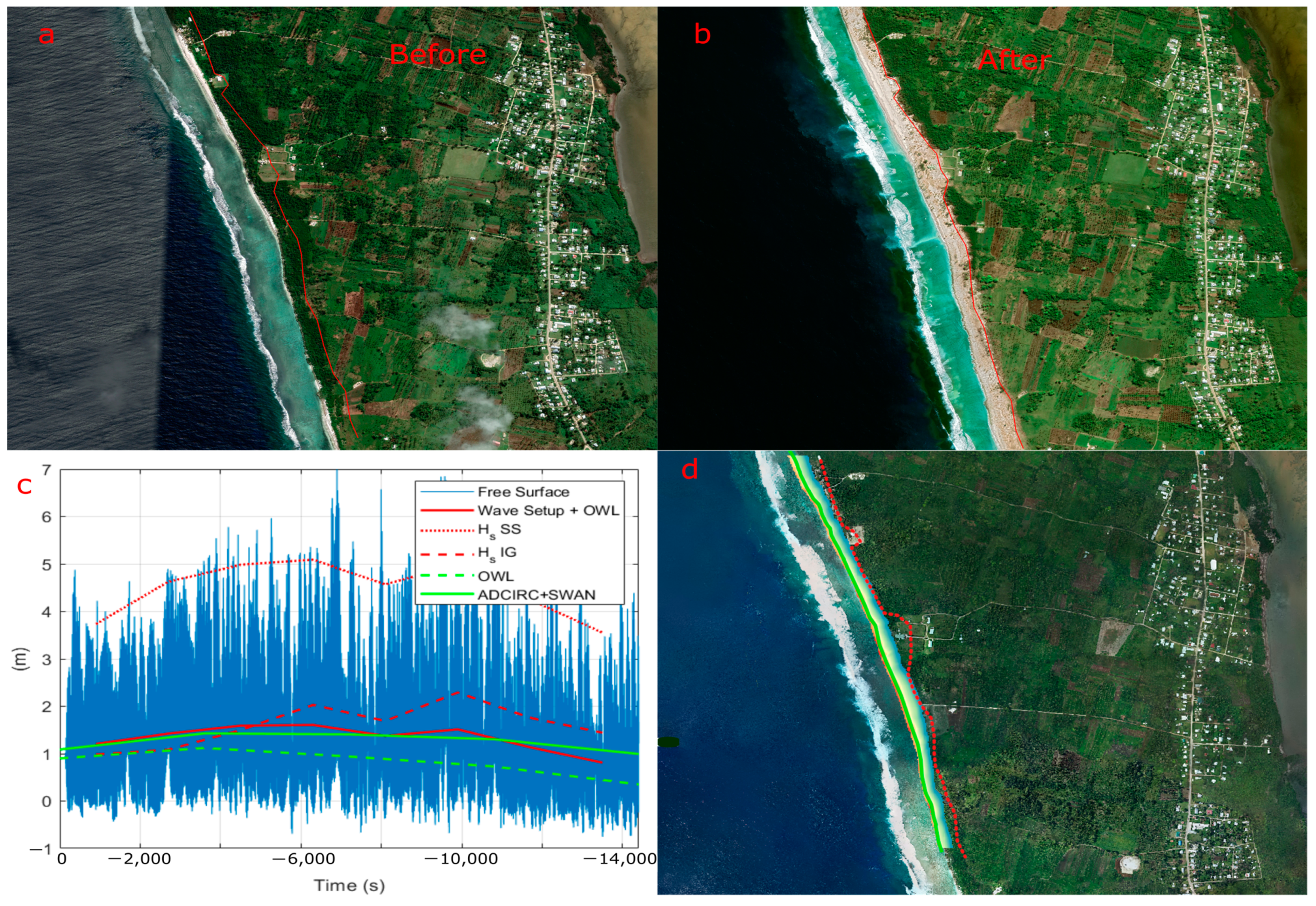
3.6. Total Water Level and Coastal Inundation
4. Conclusions
Author Contributions
Funding
Institutional Review Board Statement
Informed Consent Statement
Data Availability Statement
Acknowledgments
Conflicts of Interest
| 1 | Storm surge is the elevation in sea levels due to the combined effects of inverted barometric pressures and wind stress associated with a passage of a TC. |
| 2 | Storm tide is the water level that results from the combination of the storm surge and the astronomical tide. |
References
- World Bank. Pacific Catastrophe Risk. Assessment and Financing Initiative (PCRAFI) Project. 2007. Available online: https://documents1.worldbank.org/curated/en/251921468291332622/pdf/949860WP0Box38000Country0Note0Tonga.pdf (accessed on 20 April 2022).
- Terry, J.P. Tropical Cyclones: Climatology and Impacts in the South Pacific; Springer Science & Business Media: New York, NY, USA, 2007. [Google Scholar]
- Chand, S.S.; Walsh, K.J. Tropical cyclone activity in the Fiji region: Spatial patterns and relationship to large-scale circulation. J. Clim. 2009, 22, 3877–3893. [Google Scholar] [CrossRef]
- Needham, H.F.; Keim, B.D.; Sathiaraj, D. A review of tropical cyclone-generated storm surges: Global data sources, observations, and impacts. Rev. Geophys. 2015, 53, 545–591. [Google Scholar] [CrossRef]
- Quataert, E.; Storlazzi, C.; van Rooijen, A.; Cheriton, O.; van Dongeren, A. The Influence of Coral Reefs and Climate Change on Wave-Driven Flooding of Tropical Coastlines. Geophys. Res. Lett. 2015, 42, 6407–6415. [Google Scholar] [CrossRef]
- Vitousek, S.; Barnard, P.L.; Fletcher, C.H.; Frazer, N.; Erikson, L.; Storlazzi, C.D. Doubling of Coastal Flooding Frequency within Decades due to Sea-Level Rise. Sci. Rep. 2017, 7, 1399. [Google Scholar] [CrossRef] [PubMed]
- Church, J.A.; White, N.J.; Hunter, J.R. Sea-Level Rise at Tropical Pacific and Indian Ocean Islands. Glob. Planet. Chang. 2006, 53, 155–168. [Google Scholar] [CrossRef]
- Nurse, L.A.; McLean, R.F.; Agard, J.; Briguglio, L.P.; Duvat-Magnan, V.; Pelesikoti, N.; Tompkins, E.; Webb, A. Small islands. In Climate Change 2014: Impacts, Adaptation, and Vulnerability. Part B: Regional Aspects. Contribution of Working Group II to the Fifth Assessment Report of the Intergovernmental Panel on Climate Change; Cambridge University Press: Cambridge, UK, 2014; pp. 1613–1654. [Google Scholar]
- Nerem, R.S.; Beckley, B.D.; Fasullo, J.T.; Hamlington, B.D.; Masters, D.; Mitchum, G.T. Climate-change–driven accelerated sea-level rise detected in the altimeter era. Proc. Natl. Acad. Sci. USA 2018, 115, 2022–2025. [Google Scholar] [CrossRef]
- Begg, Z.; Damlamian, H. COSPPac Wave Climate Reports; Pacific Community (SPC): Nuku’alofa, Tonga, 2022; Available online: https://oceanportal.spc.int/portal/library/ (accessed on 20 April 2022).
- WMO. State of the Climate in the South-West Pacific 2021; WMO-No. 1302; World Meteorological Organization: Geneva, Switzerland, 2022. [Google Scholar]
- von Schuckmann, K.; Le Traon, P.Y.; Smith, N.; Pascual, A.; Djavidnia, S.; Gattuso, J.P.; Grégoire, M.; Aaboe, S.; Alari, V.; Alexander, B.E.; et al. Copernicus marine service ocean state report, issue 5. J. Oper. Oceanogr. 2021, 14 (Suppl. 1), 1–185. [Google Scholar] [CrossRef]
- Kuleshov, Y.; Qi, L.; Fawcett, R.; Jones, D. On tropical cyclone activity in the Southern Hemisphere: Trends and the ENSO connection. Geophys. Res. Lett. 2008, 35, 1–5. [Google Scholar] [CrossRef]
- Murakami, H.; Delworth, T.L.; Cooke, W.F.; Zhao, M.; Xiang, B.; Hsu, P.C. Detected climatic change in global distribution of tropical cyclones. Proc. Natl. Acad. Sci. USA 2020, 117, 10706–10714. [Google Scholar] [CrossRef]
- Knutson, T.R.; Chung, M.V.; Vecchi, G.; Sun, J.; Hsieh, T.L.; Smith, A.J. Climate change is probably increasing the intensity of tropical cyclones. Crit. Issues Clim. Chang. Sci. Sci. Brief Rev. 2021. [Google Scholar] [CrossRef]
- Andrew, N.L.; Bright, P.; de la Rua, L.; Teoh, S.J.; Vickers, M. Coastal proximity of populations in 22 Pacific Island Countries and Territories. PLoS ONE 2019, 14, e0223249. [Google Scholar] [CrossRef] [PubMed]
- Kumar, L.; Taylor, S. Exposure of coastal built assets in the South Pacific to climate risks. Nat. Clim. Change 2015, 5, 992–996. [Google Scholar] [CrossRef]
- Christensen, J.H.; Kanikicharla, K.K.; Aldrian, E.; An, S.I.; Cavalcanti, I.F.A.; de Castro, M.; Dong, W.; Goswami, P.; Hall, A.; Kanyanga, J.K.; et al. Climate phenomena and their relevance for future regional climate change. In Climate Change 2013 the Physical Science Basis: Working Group I Contribution to the Fifth Assessment Report of the Intergovernmental Panel on Climate Change; Cambridge University Press: Cambridge, UK, 2013; pp. 1217–11308. [Google Scholar]
- Walsh, K.J.; McBride, J.L.; Klotzbach, P.J.; Balachandran, S.; Camargo, S.J.; Holland, G.; Knutson, T.R.; Kossin, J.P.; Lee, T.C.; Sobel, A.; et al. Tropical cyclones and climate change. Wiley Interdiscip. Rev. Clim. Chang. 2016, 7, 65–89. [Google Scholar] [CrossRef]
- Knutson, T.; Camargo, S.J.; Chan, J.C.; Emanuel, K.; Ho, C.H.; Kossin, J.; Mohapatra, M.; Satoh, M.; Sugi, M.; Walsh, K.; et al. Tropical cyclones and climate change assessment: Part II: Projected response to anthropogenic warming. Bull. Am. Meteorol. Soc. 2020, 101, E303–E322. [Google Scholar] [CrossRef]
- Kohno, N.; Dube, S.K.; Entel, M.; Fakhruddin, S.H.M.; Greenslade, D.; Leroux, M.D.; Rhome, J.; Thuy, N.B. Recent progress in storm surge forecasting. Trop. Cyclone Res. Rev. 2018, 7, 128–139. [Google Scholar]
- Winter, G.; Storlazzi, C.; Vitousek, S.; van Dongeren, A.; McCall, R.; Hoeke, R.; Skirving, W.; Marra, J.; Reyns, J.; Aucan, J.; et al. Steps to Develop Early Warning Systems and Future Scenarios of Storm Wave-Driven Flooding Along Coral Reef-Lined Coasts. Front. Mar. Sci. 2020, 7, 1–8. [Google Scholar] [CrossRef]
- Zheng, L.; Weisberg, R.H. Modeling the west Florida coastal ocean by downscaling from the deep ocean, across the continental shelf and into the estuaries. Ocean Model. 2012, 48, 10–29. [Google Scholar] [CrossRef]
- Kerr, P.C.; Martyr, R.C.; Donahue, A.S.; Hope, M.E.; Westerink, J.J.; Luettich, R.A., Jr.; Kennedy, A.B.; Dietrich, J.C.; Dawson, C.; Westerink, H.J. US IOOS coastal and ocean modeling testbed: Evaluation of tide, wave, and hurricane surge response sensitivities to mesh resolution and friction in the Gulf of Mexico. J. Geophys. Res. Ocean. 2013, 118, 4633–4661. [Google Scholar] [CrossRef]
- Kennedy, A.B.; Westerink, J.J.; Smith, J.M.; Hope, M.E.; Hartman, M.; Taflanidis, A.A.; Tanaka, S.; Westerink, H.; Cheung, K.F.; Smith, T.; et al. Tropical cyclone inundation potential on the Hawaiian Islands of Oahu and Kauai. Ocean Model. 2012, 52, 54–68. [Google Scholar] [CrossRef]
- Hoeke, R.K.; McInnes, K.L.; O’Grady, J.; Lipkin, F.; Colberg, F. High Resolution Met-Ocean Modelling for Storm Surge Risk Analysis in Apia, Samoa. In CAWCR Technical Report. 071; The Centre for Australian Weather and Climate Research: Melbourne, Australia, 2014. Available online: https://www.cawcr.gov.au/technical-reports/CTR_071.pdf (accessed on 20 June 2021).
- Joyce, B.R.; Gonzalez-Lopez, J.; Van der Westhuysen, A.J.; Yang, D.; Pringle, W.J.; Westerink, J.J.; Cox, A.T. US IOOS coastal and ocean modeling testbed: Hurricane-induced winds, waves, and surge for deep ocean, reef-fringed islands in the Caribbean. J. Geophys. Res. Ocean. 2019, 124, 2876–2907. [Google Scholar] [CrossRef]
- Luettich, R.A.; Westerink, J.J.; Scheffner, N.W. ADCIRC: An advanced three-dimensional circulation model for shelves, coasts, and estuaries. Report 1. In Theory and Methodology of ADCIRC-2DDI and ADCIRC-3DL; Coastal Engineering Research Center: Vicksburg, MS, USA, 1992. [Google Scholar]
- Booij, N.; Holthuijsen, L.H.; Ris, R.C. The “SWAN” wave model for shallow water. Coast. Eng. Proc. 1996, 1, 668–676. [Google Scholar]
- Fleming, J.G.; Fulcher, C.W.; Luettich, R.A.; Estrade, B.D.; Allen, G.D.; Winer, H.S. A Real Time Storm Surge Forecasting System using ADCIRC. In Proceedings of the 10th International Conference on Estuarine and Coastal Modeling, Reston, VA, USA, 5–7 November 2007; pp. 893–912. [Google Scholar]
- Dietrich, J.C.; Tanaka, S.; Westerink, J.J.; Dawson, C.N.; Luettich, R.A.; Zijlema, M.; Holthuijsen, L.H.; Smith, J.M.; Westerink, L.G.; Westerink, H.J. Performance of the unstructured-mesh, SWAN ADCIRC model in computing hurricane waves and surge. J. Sci. Comput. 2012, 52, 468–497. [Google Scholar] [CrossRef]
- Ferreira, C.M.; Irish, J.L.; Olivera, F. Uncertainty in hurricane surge simulation due to land cover specification. J. Geophys. Res. Ocean. 2014, 119, 1812–1827. [Google Scholar] [CrossRef]
- Deb, M.; Ferreira, C.M. Potential impacts of the Sunderban mangrove degradation on future coastal flooding in Bangladesh. J. Hydro-Environ. Res. 2017, 17, 30–46. [Google Scholar] [CrossRef]
- Dietrich, J.C.; Bunya, S.; Westerink, J.J.; Ebersole, B.A.; Smith, J.M.; Atkinson, J.H.; Jensen, R.; Resio, D.T.; Luettich, R.A.; Dawson, C.; et al. A high-resolution coupled riverine flow, tide, wind, wind wave, and storm surge model for southern Louisiana and Mississippi. Part II: Synoptic description and analysis of Hurricanes Katrina and Rita. Mon. Weather Rev. 2010, 138, 378–404. [Google Scholar] [CrossRef]
- Reddy, M.S.D. TROPICAL CYCLONE ‘ISAAC’, 28 FEBRUARY-3 MARCH 1982. Weather Clim. 1983, 3, 32–35. [Google Scholar] [CrossRef]
- Hoeke, R.K.; McInnes, K.L.; Kruger, J.C.; McNaught, R.J.; Hunter, J.R.; Smithers, S.G. Widespread Inundation of Pacific Islands Triggered by Distant-Source Wind-Waves. Glob. Planet. Change 2013, 108, 128–138. [Google Scholar] [CrossRef]
- McInnes, K.L.; Walsh, K.J.; Hoeke, R.K.; O’Grady, J.G.; Colberg, F.; Hubbert, G.D. Quantifying storm tide risk in Fiji due to climate variability and change. Glob. Planet. Change 2014, 116, 115–129. [Google Scholar] [CrossRef]
- Mattocks, C.; Forbes, C. A real-time, event-triggered storm surge forecasting system for the state of North Carolina. Ocean Model. 2008, 25, 95–119. [Google Scholar] [CrossRef]
- Lakshmi, D.D.; Murty, P.; Bhaskaran, P.K.; Sahoo, B.; Kumar, T.S.; Shenoi, S.; Srikanth, A. Performance of WRF-ARW winds on computed storm surge using hydrodynamic model for Phailin and Hudhud Cyclones. Ocean Eng. 2017, 131, 135–148. [Google Scholar] [CrossRef]
- Ao, J.C.; Muhammad, A.; Curcic, M.; Fathi, A.; Dawson, C.N.; Chen, S.S.; Luettich, R.A., Jr. Sensitivity of storm surge predictions to atmospheric forcing during Hurricane Isaac. J. Waterw. Port Coast. Ocean Eng. 2018, 144, 04017035. [Google Scholar]
- Holland, R.W. An analytic model of the wind and pressure profiles in hurricanes. Mon. Weather Rev. 1980, 108, 1212–1218. [Google Scholar] [CrossRef]
- Gao, J. On the Surface wind Stress for Storm Surge Modeling. Doctoral Dissertation, The University of North Carolina at Chapel Hill, Chapel Hill, NC, USA, 2018. [Google Scholar]
- Ramos Valle, A.N.; Curchitser, E.N.; Bruyere, C.L.; Fossell, K.R. Simulating storm surge impacts with a coupled atmosphere-inundation model with varying meteorological forcing. J. Mar. Sci. Eng. 2018, 6, 35. [Google Scholar] [CrossRef]
- Powell, M.D.; Murillo, S.; Dodge, P.; Uhlhorn, E.; Gamache, J.; Cardone, V.; Cox, A.; Otero, S.; Carrasco, N.; Annane, B.; et al. Reconstruction of Hurricane Katrina’s wind fields for storm surge and wave hindcasting. Ocean. Eng. 2010, 37, 26–36. [Google Scholar] [CrossRef]
- Yin, J.; Lin, N.; Yu, D.P. Coupled modeling of storm surge and coastal inundation: A case study in New York city during hurricane sandy. Water Resour. Res. 2016, 52, 8685–8699. [Google Scholar] [CrossRef]
- Velissariou, P.; Moghimi, S. Parametric Hurricane Modeling System (PaHM) Manual; NOAA: Washington, DC, USA, 2022.
- Reardon, G.F.; Oliver, J. Report on Damage Caused by Cyclone Isaac in Tonga; Department of Civil & Systems Engineering, James Cook University: Townsville, Australia, 1982. [Google Scholar]
- Mimura, N.; Pelesikoti, N. Vulnerability of Tonga to future sea-level rise. J. Coast. Res. 1997, 24, 117–132. Available online: http://www.jstor.org/stable/25736091 (accessed on 30 July 2022).
- Department of Foreign Affairs and Trade. Crisis Hub-TC Harold. 2020. Available online: https://www.dfat.gov.au/crisis-hub/tropical-cyclone-harold (accessed on 25 May 2023).
- Tonga Meteorological Service. Meteorological Report on Severe Tropical Cyclone “Harold” (Category 4) 7th–9th April 2020; Nuku’alofa, Tonga, 2020. Available online: https://met.gov.to/wp-content/uploads/2021/11/TC_HAROLD-REPORT.pdf (accessed on 30 June 2022).
- Cylone Harold. 2020. Available online: https://en.wikipedia.org/wiki/Cyclone_Harold#:~:text=On%20April%2023%2C%20Tonga’s%20Minister,excess%20of%20US%24111%20million (accessed on 20 April 2022).
- Merrifield, M.A.; Becker, J.M.; Ford, M.; Yao, Y. Observations and estimates of wave-driven water level extremes at the Marshall Islands. Geophys. Res. Lett. 2014, 41, 7245–7253. [Google Scholar] [CrossRef]
- Wandres, M.; Aucan, J.; Espejo, A.; Jackson, N.; De Ramon N’Yeurt, A.; Damlamian, H. Distant-source swells cause coastal inundation on Fiji’s Coral Coast. Front. Mar. Sci. 2020, 7, 546. [Google Scholar] [CrossRef]
- Hoeke, R.K.; Damlamian, H.; Aucan, J.; Wandres, M. Severe flooding in the atoll nations of Tuvalu and Kiribati triggered by a distant tropical cyclone pam. Front. Mar. Sci. 2021, 7, 539646. [Google Scholar] [CrossRef]
- Tu’uholoaki, M.; Singh, A.; Espejo, A.; Chand, S.; Damlamian, H. Tropical cyclone climatology, variability, and trends in the Tonga region, Southwest Pacific. Weather Clim. Extrem. 2022, 37, 100483. [Google Scholar] [CrossRef]
- Roelvink, D.; Reniers, A.; van Dongeren, A.; van Thiel de Vries, J.; McCall, R.; Lescinski, J. Modelling storm impacts on beaches, dunes and barrier islands. Coast. Eng. 2009, 56, 1133–1152. [Google Scholar] [CrossRef]
- Luick, J.L.; Henry, R.F. Tides in the Tongan region of the pacific ocean. Mar. Geod. 2000, 23, 17–29. [Google Scholar] [CrossRef]
- Bosserelle, C.; Reddy, S.; Lal, D. Waves and Coast in the Pacific (WACOP) Wave Climate Reports; Pacific Community: Suva, Fiji, 2015. [Google Scholar]
- Stephens, S.A.; Ramsay, D.L. Extreme cyclone wave climate in the Southwest Pacific Ocean: Influence of the El Niño Southern Oscillation and projected climate change. Glob. Planet. Chang. 2014, 123, 13–26. [Google Scholar] [CrossRef]
- Knapp, K.R.; Diamond, H.J.; Kossin, J.P.; Kruk, M.C.; Schreck, C.J. International Best Track Archive for Climate Stewardship (IBTrACS) Project, Version 4. [Indicate Subset Used]; NOAA National Centers for Environmental Information: Kiln, MS, USA, 2018. [CrossRef]
- Diamond, H.J.; Lorrey, A.M.; Knapp, K.R.; Levinson, D.H. Development of an enhanced tropical cyclone tracks database for the southwest Pacific from 1840 to 2010. Int. J. Climatol. 2012, 32, 2240–2250. [Google Scholar] [CrossRef]
- Roberts, K.J.; Pringle, W.J.; Westerink, J.J. OceanMesh2D 1.0: MATLAB-based software for two-dimensional unstructured mesh generation in coastal ocean modeling. Geosci. Model Dev. 2019, 12, 1847–1868. [Google Scholar] [CrossRef]
- Tozer, B.; Sandwell, D.T.; Smith, W.H.F.; Olson, C.; Beale, J.R.; Wessel, P. Global Bathymetry and Topography at 15 Arc Sec: SRTM15+. Earth Space Sci. 2019, 6, 1847–1864. [Google Scholar] [CrossRef]
- Aydoğan, B.; Ayat, B. Performance evaluation of SWAN ST6 physics forced by ERA5 wind fields for wave prediction in an enclosed basin. Ocean. Eng. 2021, 240, 109936. [Google Scholar] [CrossRef]
- Rogers, W.E.; Hwang, P.A.; Wang, D.W. Investigation of wave growth and decay in the SWAN model: Three regional-scale applications. J. Phys. Oceanogr. 2003, 33, 366–389. [Google Scholar] [CrossRef]
- Nelson, R.C. Depth limited design wave heights in very flat regions. Coast. Eng. 1994, 23, 43–59. [Google Scholar] [CrossRef]
- Madsen, O.S.; Rosengaus, M.M. Spectral wave attenuation by bottom friction: Experiments. In Coastal Engineering; American Society of Civil Engineers: Reston, VA, USA, 1988; pp. 849–857. [Google Scholar]
- Hasselmann, K.; Barnett, T.P.; Bouws, E.; Carlson, H.; Cartwright, D.E.; Enke, K.; Ewing, J.A.; Gienapp, A.; Hasselmann, D.E.; Kruseman, P.; et al. Measurements of wind-wave growth and swell decay during the Joint North Sea Wave Project (JONSWAP). Ergaenzungsheft Zur Dtsch. Hydrogr. Z. Reihe A 1973. Available online: http://resolver.tudelft.nl/uuid:f204e188-13b9-49d8-a6dc-4fb7c20562fc (accessed on 19 July 2022).
- Garratt, J.R. Review of drag coefficients over oceans and continents. Mon. Weather Rev. 1977, 105, 915–929. [Google Scholar] [CrossRef]
- Lashley, C.H.; Roelvink, D.; van Dongeren, A.; Buckley, M.L.; Lowe, R.J. Nonhydrostatic and surfbeat model predictions of extreme wave run-up in fringing reef environments. Coast. Eng. 2018, 137, 11–27. [Google Scholar] [CrossRef]
- Ford, M.; Merrifield, M.A.; Becker, J.M. Inundation of a low-lying urban atoll island: Majuro, Marshall Islands. Nat. Hazards 2018, 91, 1273–1297. [Google Scholar] [CrossRef]
- Funakoshi, Y.; Hagen, S.C.; Bacopoulos, P. Coupling of hydrody- namic and wave models: Case study for Hurricane Floyd (1999) hindcast. ASCE J. Waterw. Port Coast. Ocean Eng 2008, 134, 321–335. [Google Scholar] [CrossRef]
- Cyclone Harold. 2020. Available online: https://matangitonga.to/2020/04/15/satellite-tc-harold (accessed on 6 April 2023).
- Akbar, M.K.; Kanjanda, S.; Musinguzi, A. Effect of Bottom Friction, Wind Drag Coefficient, and Meteorological Forcing in Hindcast of Hurricane Rita Storm Surge Using SWAN + ADCIRC Model. J. Mar. Sci. Eng. 2017, 5, 38. [Google Scholar] [CrossRef]
- Camus, P.; Mendez, F.J.; Medina, R. A hybrid efficient method to downscale wave climate to coastal areas. Coast. Eng. 2011, 58, 851–862. [Google Scholar] [CrossRef]
- Rueda, A.; Cagigal, L.; Pearson, S.; Antolínez, J.A.; Storlazzi, C.; van Dongeren, A.; Camus, P.; Mendez, F.J. HyCReWW: A hybrid coral reef wave and water level metamodel. Comput. Geosci. 2019, 127, 85–90. [Google Scholar] [CrossRef]
- van Vloten, S.O.; Cagigal, L.; Rueda, A.; Ripoll, N.; Méndez, F.J. HyTCWaves: A Hybrid model for downscaling Tropical Cyclone induced extreme Waves climate. Ocean Model. 2022, 178, 102100. [Google Scholar] [CrossRef]


| Experiment (Exp.) | Model Description |
|---|---|
| 1 | ADCIRC + SWAN (astronomical tide and atmospheric forcings) |
| 2 | ADCIRC standalone (astronomical tide and atmospheric forcings) |
| 3 | ADCIR + SWAN (atmospheric forcing plus wave gradient forcing) |
| 4 | ADCIRC standalone (atmospheric forcing only) |
| 5 | ADCIRC standalone (air pressure only) |
| 6 | ADCIRC standalone (astronomical tide forcing only) |
| 7 | XBEACH to test the influence of waves on the inundation |
| Model vs. Observations | RMSE | |
|---|---|---|
| 1 | Model pressures—Figure 4 | 3.03 hPa (overall) |
| 2 | Model winds—Figure 5 | 2.84 m/s (overall) |
| 3 | Tide (COSPPac vs. ADCIRC)—Figure 6a | 0.30 cm |
| 4 | Coupled model TWL (Exp. 1)—Figure 6b | 6.7 cm |
| 5 | Uncoupled model TWL (Exp. 2)—Figure 6b | 8.9 cm |
| 6 | Model storm surge coupled run with no tide (Exp. 3)—Figure 6c | 3.5 cm |
| 7 | Model storm surge (Exp. 2–Exp. 6)—Figure 6c | 7.8 cm |
| 8 | Model storm surge (Exp. 1–Exp. 6)—Figure 6c | 4.6 cm |
| 9 | Linearly adding tide to the storm surge run without tide (Exp. 6 + Exp. 3)—Figure 6b | 7.03 cm (overall) |
Disclaimer/Publisher’s Note: The statements, opinions and data contained in all publications are solely those of the individual author(s) and contributor(s) and not of MDPI and/or the editor(s). MDPI and/or the editor(s) disclaim responsibility for any injury to people or property resulting from any ideas, methods, instructions or products referred to in the content. |
© 2023 by the authors. Licensee MDPI, Basel, Switzerland. This article is an open access article distributed under the terms and conditions of the Creative Commons Attribution (CC BY) license (https://creativecommons.org/licenses/by/4.0/).
Share and Cite
Tu’uholoaki, M.; Espejo, A.; Wandres, M.; Singh, A.; Damlamian, H.; Begg, Z. Quantifying Mechanisms Responsible for Extreme Coastal Water Levels and Flooding during Severe Tropical Cyclone Harold in Tonga, Southwest Pacific. J. Mar. Sci. Eng. 2023, 11, 1217. https://doi.org/10.3390/jmse11061217
Tu’uholoaki M, Espejo A, Wandres M, Singh A, Damlamian H, Begg Z. Quantifying Mechanisms Responsible for Extreme Coastal Water Levels and Flooding during Severe Tropical Cyclone Harold in Tonga, Southwest Pacific. Journal of Marine Science and Engineering. 2023; 11(6):1217. https://doi.org/10.3390/jmse11061217
Chicago/Turabian StyleTu’uholoaki, Moleni, Antonio Espejo, Moritz Wandres, Awnesh Singh, Herve Damlamian, and Zulfikar Begg. 2023. "Quantifying Mechanisms Responsible for Extreme Coastal Water Levels and Flooding during Severe Tropical Cyclone Harold in Tonga, Southwest Pacific" Journal of Marine Science and Engineering 11, no. 6: 1217. https://doi.org/10.3390/jmse11061217
APA StyleTu’uholoaki, M., Espejo, A., Wandres, M., Singh, A., Damlamian, H., & Begg, Z. (2023). Quantifying Mechanisms Responsible for Extreme Coastal Water Levels and Flooding during Severe Tropical Cyclone Harold in Tonga, Southwest Pacific. Journal of Marine Science and Engineering, 11(6), 1217. https://doi.org/10.3390/jmse11061217