Coastal Flood at Gâvres (Brittany, France): A Simulated Dataset to Support Risk Management and Metamodels Development

Abstract

Given recent scientific advances, coastal flooding events can be modelled even in complex environments. However, such models are computationally expensive, preventing their use for forecasting. At the same time, metamodelling techniques have been explored for coastal hydrodynamics, showing promising results. Developing such techniques for predicting coastal flood information (e.g., inland water depths) requires large enough learning datasets providing such inland information. However, detailed inland coastal flood observations are scarce and—when available—only correspond to a limited number of events. This paper aims at demonstrating how we can fill this gap by introducing a publicly available dataset, presenting its setup, and providing examples of use and recommendations. It has been built for the site of Gâvres (France), relying on the joint use of spectral wave (WW3) and non-hydrostatic wave-flow (SWASH) models, accounting for wave overtopping. It compiles 250 scenarios (defined by time-varying forcing conditions; including real and stochastically generated events) and the resulting maximal flooded areas and water depths (on 64,618 inland points). Its construction required the equivalent of 2 years of simulations on 48 cores. The examples of use of the dataset focus on method developments (metamodelling, forecast), local knowledge, and risk management.

1. Introduction

Coastal flooding is characterised by the complexity of the processes leading to flood events but also by a lack of observations inland (such as water depths, for instance). Indeed, coastal flooding is generally caused by a combination of high water levels—which may be caused by tides and storm surges—together with waves, which can lead to the overtopping of coastal defences and inundation of low-lying areas, potentially causing damage to life and property [1]. In addition, along most coastal areas, detailed flood information (e.g., flooded surface or inland water depths) is very scarce, and it is available only for a limited number of events. However, given recent scientific advances, coastal flooding events can now be properly modelled, even in complex environments and under the action of wave overtopping [2,3,4]. Such progress opens the perspective of improving our processes’ understanding (see, e.g., [2,5] for nearshore and inland processes, respectively) but also several steps of the risk management cycle, from prevention to crisis preparation, including forecasts and early warning systems (FEWSs). However, these numerical models are computationally expensive, limiting their use for early warning systems, one instrument for crisis preparation. At the same time, metamodelling techniques (also named surrogate modelling in the literature) have been explored for coastal hydrodynamics and coastal water level predictions [6,7,8,9] and have shown promising results. They are based on approaches such as kriging (see, e.g., [6]) or artificial neural networks, for instance (see, e.g., [9]). Metamodels are functions that aim to reproduce the behaviour of a “true” model (e.g., a numerical hydrodynamic model) for given input variables (for instance, offshore conditions). Their main advantage is their reduced computation time, which may be of a few seconds to minutes instead of several days for the “true” model, even using high-performance computing [10]. However, their setup requires the availability of learning datasets, datasets that are presently missing, especially when aiming to predict inland information (e.g., flooded surface, map of inland water depth).

To fill this gap, a method has been designed, allowing the construction of a simulated flood dataset (named CFMDG for Coastal Flood Modeling Dataset in Gâvres) for the site of Gâvres (Brittany, France) within the RISCOPE research project (see [10] for an overview). It relies on the joint use of a spectral wave model named WW3 [11], a non-hydrostatic wave-flow model named SWASH [12], historical data, and statistical methods.

The objective of the current paper is threefold: (1) provide a detailed description of the developed method used to build this flood dataset for the sake of application to other sites; (2) provide an accessible dataset of use for method developments (metamodelling, forecast), site-specific process knowledge, and risk management purposes; (3) provide examples of use. The CFMDG dataset is publicly available at https://zenodo.org/record/7533336#.Y-3j8XbMKUk, accessed on 13 June 2023 [13].

It should be noted that previous non-publicly available versions of the CFMDG dataset have been already used to develop a forecast and early warning prototype, relying on metamodelling approaches [10]. However, no extensive description of the dataset and the method developed to build it was provided. In addition, as illustrated in the present manuscript, such datasets can be useful for other types of investigations. To provide a broad illustration of examples of use, the examples presented in this paper include this previous work (Section 3.3) but also new analyses (Section 3.2).

2. The Dataset and Methods

In this section, we first briefly describe the site and introduce the dataset (Section 2.1). Then, the method is presented (Section 2.2), and the main steps are described in more detail in the following subsections.

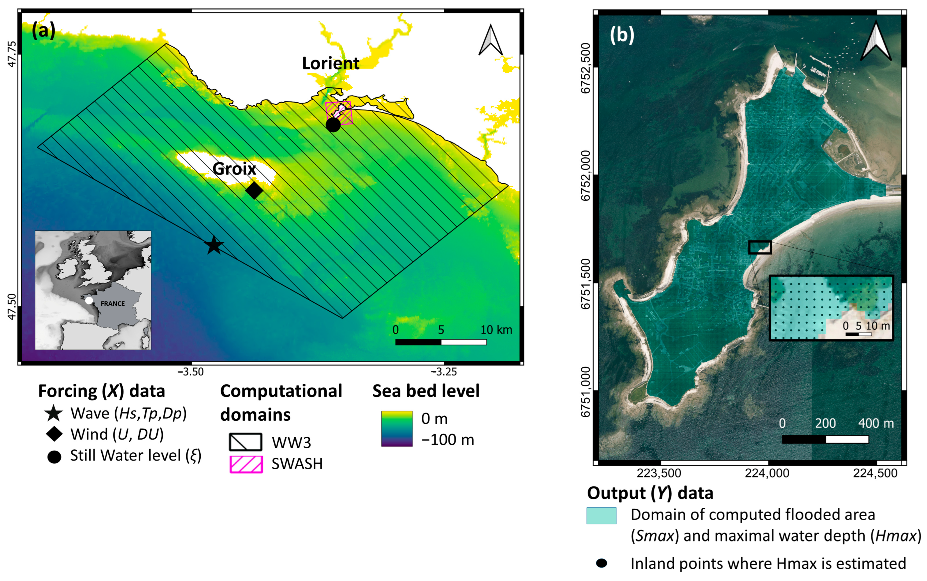
2.1. The Site and Dataset

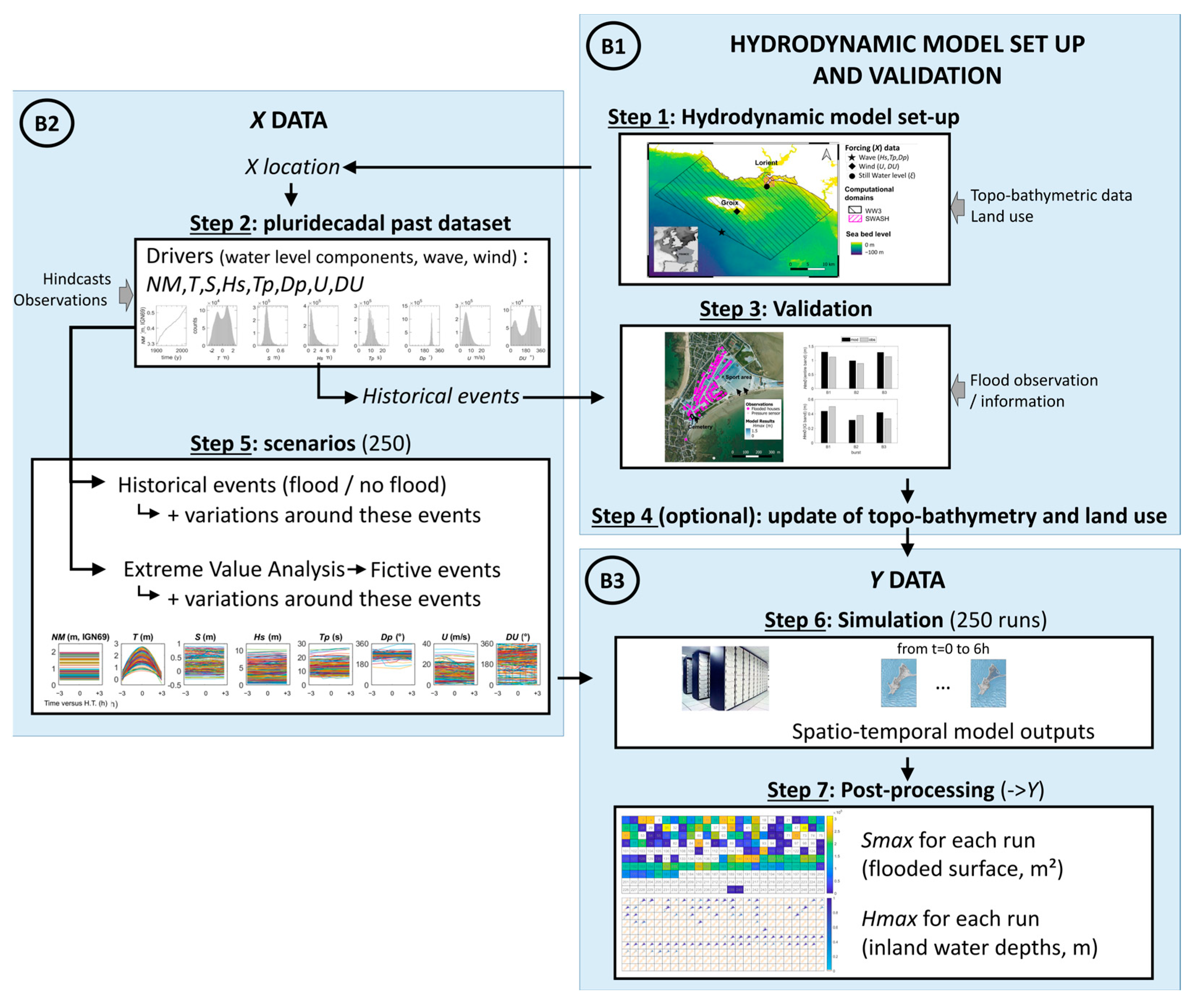
Gâvres is representative of towns presently subject to wave overtopping and presents the advantage to be a small territory (2 km²) for exploration needs. Located on the French Atlantic coast (Figure 1a), it has experienced five significant past flood events since 1900 (see [3] for a detailed analysis for the period from 1900–2010). The last major flood occurred on March 10th of 2008 (windstorm Johanna), in which approximately 120 houses were flooded (Figure 2a, purple dots).

The CFMDG dataset compiles a set of 250 scenarios and related post-processed coastal flood simulations (Figure 1a) for a digital elevation model representative of the 2018 coastal defence configuration. Each scenario is defined by a 6 h time series centred on high tide, with one time series per forcing variable. The forcing variables are: local relative mean sea level (NM), tide (T), atmospheric storm surge (S), offshore wave characteristics (significant height, Hs; peak period, Tp; peak direction, Dp), and offshore wind (speed, U; direction, DU). These scenarios combine past real events with extreme statistics-based events and some complementary fictive events. The post-processed outputs include, for each scenario, the maximal flooded area (Smax) and the maximal water depth (Hmax) in each inland model grid point (grid cell size of 3 m). The data described here were partly used in previous publications to develop metamodels, allowing the prediction of inland flood information, such as flooded areas [14,15] or maps of inland water depths [16], and the construction of a forecast and early warning prototype [10].

Table 1. Dataset fields for each scenario.

Variable Name	Description and Unit	Comment
sc	Number of the scenario.
INPUTS (X)
NM	Relative mean sea level, referenced to the French vertical datum (m, IGN69)	Time series over 6 h Input for the numerical simulations
T	Tidal water level (m), referenced to the relative mean sea level
S	Atmospheric storm surge (m)
Hs	Significant wave height (m)
Tp	Wave peak period (s)
Dp	Wave peak direction (° in nautical convention)
U	Wind speed (m/s)
DU	Wind direction (° in nautical convention)
t	Relative time centred on the high tide of each event (min)
High Tide date	UTC date for scenarios corresponding to past real events
OUTPUTS (Y)
Smax	Maximum flooded area during the event (m²)	Post-processed scalar output
Hmax	Maximum water depth reached during the event (m), provided for each inland location	Post-processed functional (map) output
longitude	Longitude (°, WGS84)	For each inland location point
latitude	Latitude (°, WGS84)
XL93	Longitude (m, Lambert 93)
YL93	Latitude (m, Lambert 93)

lists the fields of the dataset for each scenario. For each scenario, the following complementary information is provided in the dataset: the type of scenario (past real event, variation around a past real event, statistical event, variation around a statistical event; when the type of scenario corresponds to a variation around an event, the n° of the scenario corresponding to the concerned event is given), the date of the high tide (UTC; for past real flood), the source of the data. A detailed description of the various types of scenarios is provided in Section 2.4.

2.2. Method

Figure 2 describes the method used to build the dataset. It relies on the following 7 main steps:

• Step 1: Hydrodynamic model setup.
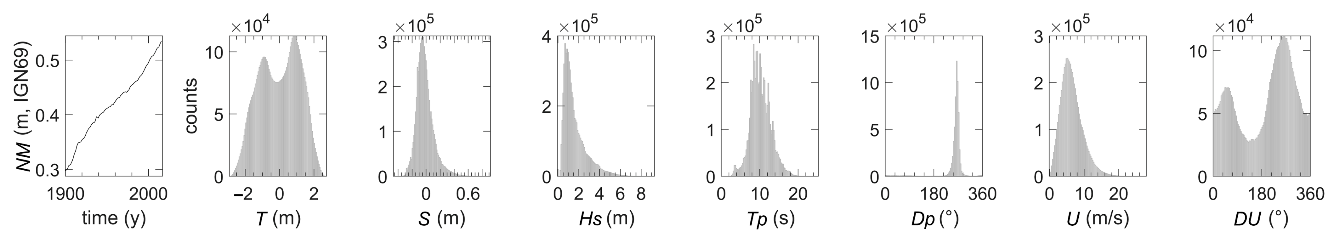
• Step 2: Constitution of a pluri-decadal past time series of the drivers (NM, T, S, Hs, Tp, Dp, U, DU) at the locations of forcing for the modelling chain.
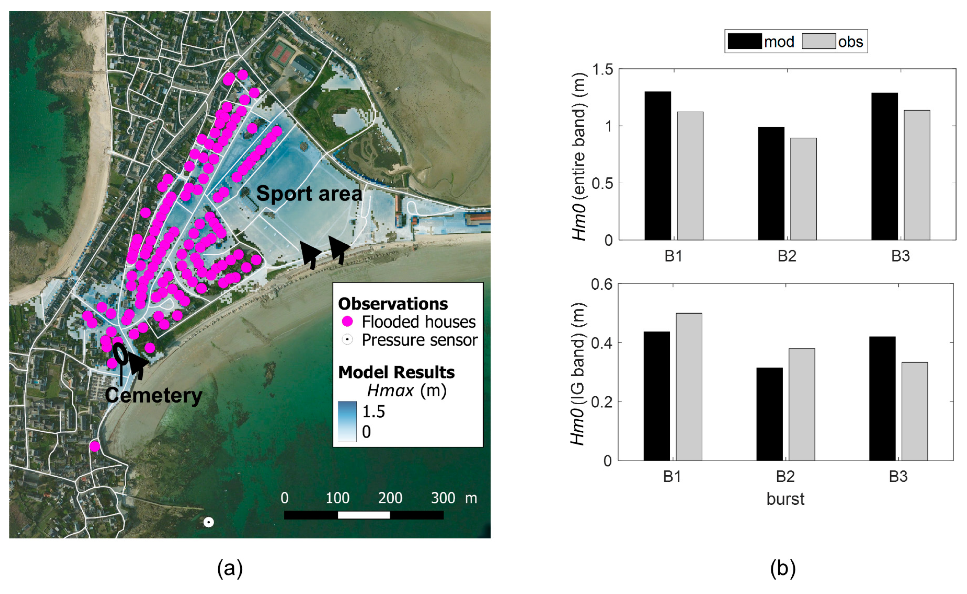
• Step 3: Validation of the modelling chain on past real events.
• Step 4 (optional): Update of the topo-bathymetry and land use in the model.
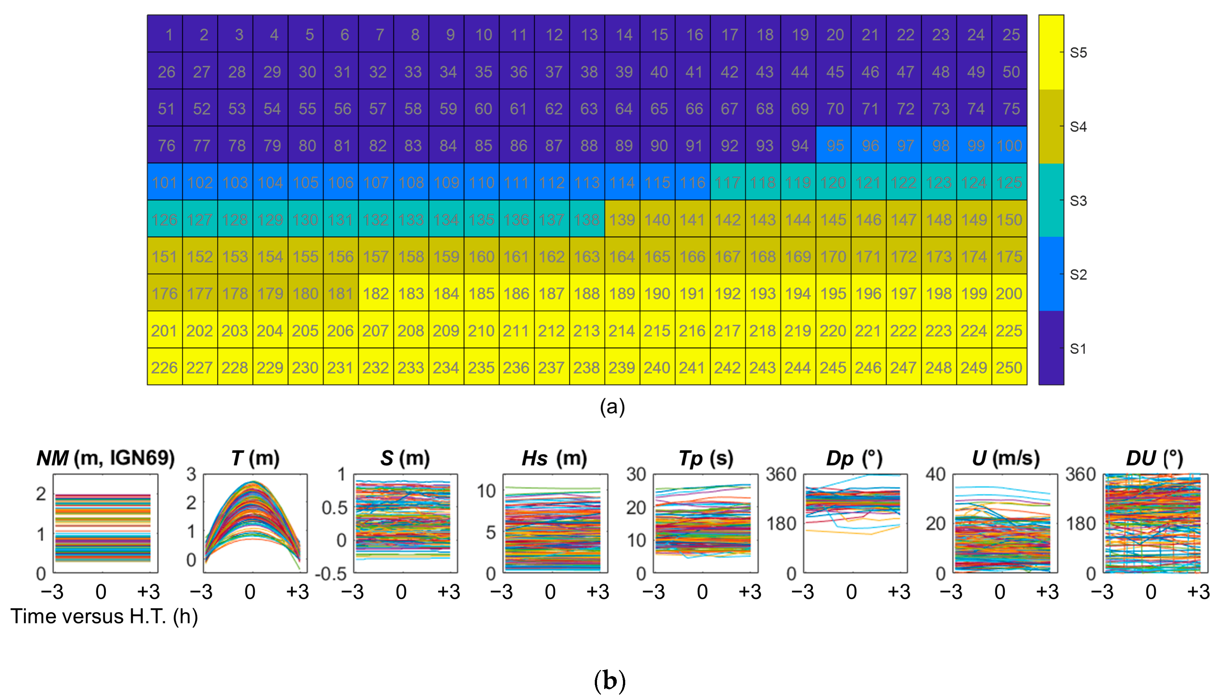
• Step 5: Definition of the scenarios (here, 250) of forcing conditions (X).
• Step 6: Simulation with the hydrodynamic modelling chain for the 250 scenarios.
• Step 7: Post-processing to provide the synthetic outputs (Y).

These steps are part of the following three main blocks:

• Block 1: The hydrodynamic model setup, validation (and update).
• Block 2: The X data and design of the scenarios to be used in the simulations.
• Block 3: The Y data, obtained by simulations and post-processing of the model outputs.

The next subsections describe in more detail these three blocks.

2.3. Block 1: Coastal Flood Model Setup and Validation

To produce the CFMDG dataset, we used the non-hydrostatic phase-resolving model SWASH [12] to model floods at the study site. The modelling chain was previously set up by Idier et al. [3,4]. We briefly summarise the key elements here. First, the wave conditions offshore of Groix (Hs, Tp, Dp) are downscaled to the boundaries of the SWASH model (Figure 1) using the WW3 spectral wave model [11] by adopting the Jonswap wave spectrum with a directional spread of 30° and taking into account the local wind (U, DU) and still water level (named ξ, with ξ = NM + T + S). The WW3 computational domain is shown in Figure 1a (in black). SWASH is run with non-uniform wave boundary conditions and spatially uniform still water levels (ξ, resulting from spatially uniform mean sea level, tides, and atmospheric surges) and wind (U, DU). The spatial and temporal resolutions of SWASH are 3 m and more than 10 Hz, respectively. In the vertical direction, a two-layer discretisation is used. The spatial variability in the bottom roughness (related to land use) is taken into account following the same approach as in [2]. This model chain was validated in terms of the flooded area observed during the 10th March 2008 storm event [3]. For this validation (Step 3, Figure 2), the model was run for a digital elevation model (DEM) representative of the 2008 period (denoted DEM2008) over a 6 h window (centred on high tide) using simulated water level data produced by Le Roy et al. [2] and wave and wind conditions extracted from a hydro-meteorological dataset covering the 1900–2016 period and built using post-processing (correcting) surge, wave, and meteorological hindcasts ([3], Step 2 of the method, see Section 2.4). Figure 3a shows the reasonable agreement between the modelled maximal inland water depths during the event and the observed counterpart (flooded houses in purple). As a complement, the ability of the same modelling chain to detect past flooding/non-flooding events over the 1900–2010 period was demonstrated by Idier et al. [3]. Validation of the simulated nearshore high-frequency (f > 1 Hz) water levels was also performed under more moderate conditions (2018–2019), showing good agreement with in situ measurements for both gravity and infragravity bands (Figure 3b; [17]).

For the needs of the RISCOPE project (forecast), as the topo-bathymetry has significantly changed since 2008 due to—among other factors—beach nourishment and the heightening of some coastal defences, we used the above-mentioned model chain, but we included a DEM that better represents the present-day configuration (Step 4, Figure 2). From the available bathymetric surveys (provided by the French Hydrographic Hydrographic and Oceanographic Office (SHOM) and the Danish Hydraulic Institute (DHI)), LiDAR data (public RGE ALTI^® IGN product—https://www.data.gouv.fr/fr/datasets/rge-alti/, accessed on 13 June 2023; limited access data of Lorient Agglomeration), and Global Positioning System (GPS) survey of the coastal defences, Idier et al. [10] have constructed a DEM (denoted DEM2018) that is representative of the 2015 bathymetry (winter) and 2018 coastal defences. All the simulations used to build the CFMDG dataset are performed with this DEM2018. It should be noted that Step 4 is optional, as it depends on the local evolution of the topo-bathymetry and coastal defences as well as the objective of the dataset.

2.4. Block 2: X Data and Grid Experiment Design

Table 2. Description of the types of 250 scenarios (i.e., forcing events).

Name	Type	Number of Scenarios	Scenario n°
S1	Fictive, based on extreme value analysis	94	1 to 94
S2	Past real event, inside the damage database of [3]	22	95 to 116
S3	Fictive, based on variations around real past forcing event	22	117 to 138
S4	Fictive, based on variations around an extreme-value-analysis-based event	44	139 to 182
S5	Past real event, outside the damage database of [3]	68	183 to 250

summarizes the types of scenarios (forcing conditions X) included in the CFMDG dataset. As highlighted above and detailed in Section 2.5, the computation time related to the hydrodynamic modelling limits the number of possible simulations. In the present work, the total number of simulations was initially limited to about 130. Analysing the preliminary results, other additional simulations were carried out to reach 250 scenarios.

To design realistic scenarios, we require data covering past periods (ideally several decades). This is Step 2 of the method. In the present work, we rely on the database (named HM) of hydro-meteorological data (at the X locations, Figure 1a) set up in [3] over the period from 1900–2016, with a 10 min time step resolution (Figure 4). Here, we remind briefly the method used to set up this HM dataset. As there is no tide gauge measurement close enough to the site and covering the entire study period to estimate still water levels (ξ), each component of the still water level (NM, T, S) has been estimated over the 1900–2016 period based on different types of data. For the mean sea level (relative to the land), regional tide gauge data and the 3 nearest GPS stations data have been combined to account for the vertical land motion. For the tide, it has been reconstructed using the tidal component database FES2014 [18]. For the atmospheric storm surge, waves, and wind, datasets of different qualities have been combined, and a method has been applied to reduce the bias (based on a quantile–quantile method). Appendix A provides more details on the datasets and processing used to build the HM dataset. Figure 4 shows the distribution of this continuous HM dataset over the 1900–2016 period. This dataset is used for two purposes: (1) to provide forcing conditions to the numerical model on past events for validation purposes (Step 3) and (2) to design the X scenarios (Step 5).

The first set of scenarios (Figure 2, step 5) was built as follows. First, a combination of Monte Carlo random sampling and multivariate extreme value analysis is performed on the HM dataset to provide a large dataset of extreme conditions (here, ~150,000). Then, we start by selecting a limited number of 100 offshore meteo-oceanic scalar conditions; X_S = (ξ, Hs, Tp, Dp, U, DU), as was performed by Rohmer et al. [19]. This selection is designed by applying the clustering procedure described by Gouldby et al. [20]. This approach ensures that the selected X_S input conditions are sufficiently extreme to lead to flooding but are also realistic. Then, using this first selection of X_S conditions and the 1900–2016 hydro-meteorological dataset [3], a probabilistic classifier is used to locate the time instants of these maximum values (based on quadratic discriminant analysis; [21]), and a multivariate truncated Gaussian-Monte-Carlo-based sampling procedure is applied to generate the 100 corresponding time series—i.e., functional inputs X = (NM (t), T (t), S (t), Hs (t), Tp (t), Dp (t), U (t), DU (t)), over 6 h, with 10 min time steps. Keeping in mind that SWASH is a research code, spurious numerical oscillations may sometimes affect the solutions in very tough applications and lead to simulation crashes. Thus, running the modelling chain for the 100 scenarios leads to a set of 94 usable model simulations (scenarios S1, Table 2). This first set of scenarios is completed with 21 historical forcing events (scenarios S2, Table 2) including the 9 known to have led to flooding at the study site (see [3]). It should be noted that two different scenarios—sc100 and sc116—correspond to the historical event Johanna 10/03/2008, the difference being related to the data source, leading finally to 22 scenarios pf type S2. The first set of scenario is also completed by 16 scenarios simulated from variations of the forcing conditions of the 9 historical flood events (part of scenarios S3, Table 2). This first set of time-varying forcing conditions contains 133 scenarios.

Based on a preliminary analysis of the simulations performed for the above 133 scenarios, the following complementary scenarios were designed:

• Variations around one additional given real event (thus, one additional scenario in group S3).
• Variations around fictive events, focussing on events (group S1) for which an improvement of the multi-outputs metamodels of [16] was pursued. These scenarios correspond to the scenario group S4.
• Real past conditions not having led to flood or damage events (after [3,10]), extracted from the 1900–2016 HM database of [4]) and from complementary source data (MARC/LOPS and Meteo-France for events occurring after 2016). This scenario type is denoted as S5 in Table 2.

Finally, 250 scenarios are designed (summarized in Table 2 and Figure 5a). For each X scenario, in addition to the information provided in Table 2, the following complementary information is provided: data source and scenario of reference when the considered scenario corresponds to a variation around another scenario (e.g., a past real event or a fictive event).

2.5. Block 3: Simulations and Post-Processing

Regarding Step 6 (Figure 2), all the simulations used to build the Y dataset were performed on 2.6 GHz MD Abu Dhabi and 2.4 GHz AMD Interlagos processors. The entire modelling chain (WW3-SWASH) was run on 48 cores. A single scenario run requires a computation time of 3 days to simulate 6 h on 48 cores, with SWASH representing 97% of the computation. The total computation time to build the dataset represents about 2 years of computations (3 days × 250 scenarios) on 48 cores.

Our simulations provide spatiotemporal grids of water depth over the entire SWASH domain (Figure 1a, pink box) at resolutions of 3 m and 1 min over a 6 h period. In step 7, these model outputs are post-processed in the following way: (1) computation of the maximum water depth (Hmax) in each pixel of the SWASH domain (i.e., every 3 m); (2) extraction of Hmax value and the centre of each grid cell over the inland domain of interest (Figure 1b, blue domain). This directly provides the Hmax outputs (i.e., Hmax value in Np = 64,618 points, all located inland and distributed on a regular grid, see zoom in Figure 1b). Smax is computed as the sum of inland points at which Hmax > 0, multiplied by the grid cell dimension (i.e., 3 × 3 = 9 m²).

3. Results and Examples of Use

3.1. Results: Synthetic View of the Dataset

This subsection provides a synthetic view of the built CFMDG dataset. The dataset is made of input data (X, with X = (NM, T, S, Hs, Tp, Dp, U, DU) (t)) and output data (Y, with Y = (Smax; Hmax (longitude, latitude) for the Np points)). Figure 5 and Figure 6 show a synthetic view of the X time series and Y outputs for the 250 scenarios.

To complete the synthetic view of the Hmax maps dataset, Figure 7 shows the distribution of the flood intensity (using Smax as an intensity indicator and considering 5 classes, from Smax = 0 to Smax larger than 30% of the studied area, Stot) as well as a map that shows, for each pixel, the ratio (rp) defined as the number of scenarios in which the pixel is flooded (npf) to the total number of simulations (denoted npt, with here npt = 250).

3.2. Examples of Analyses of the CFMDG Dataset

The examples provided in this subsection have been designed specifically for the present paper.

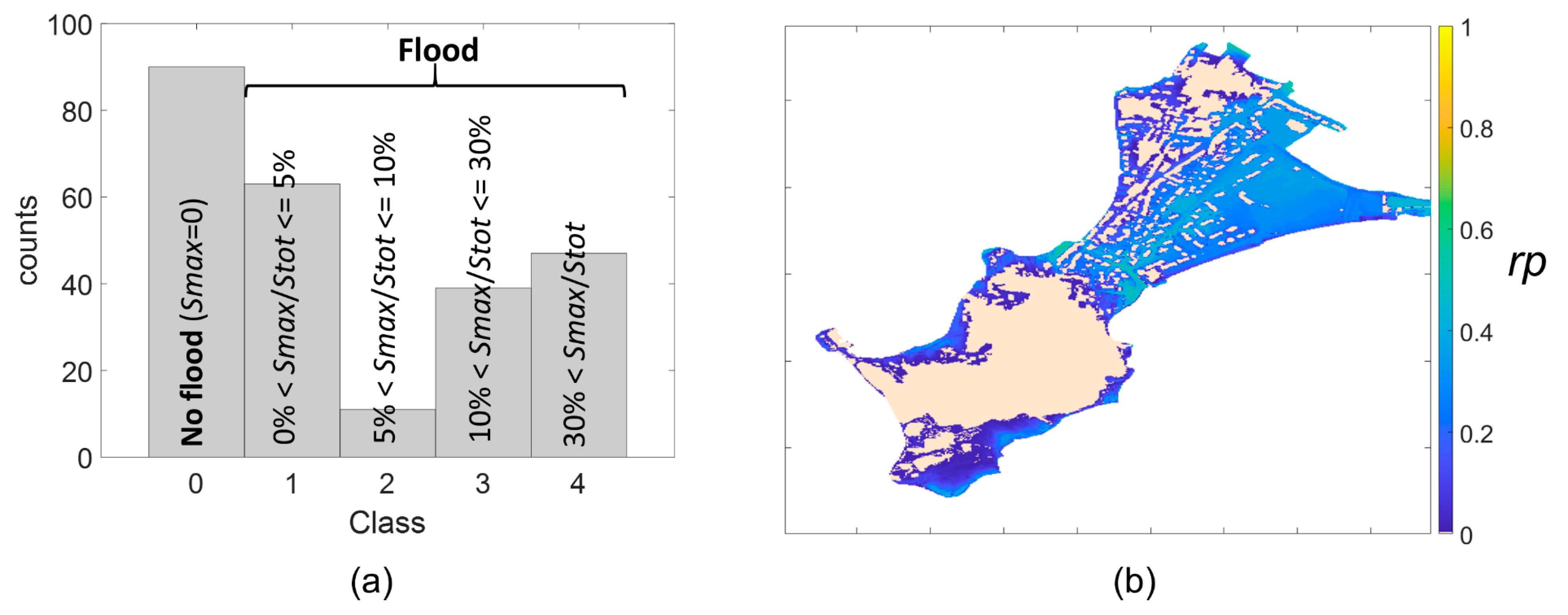
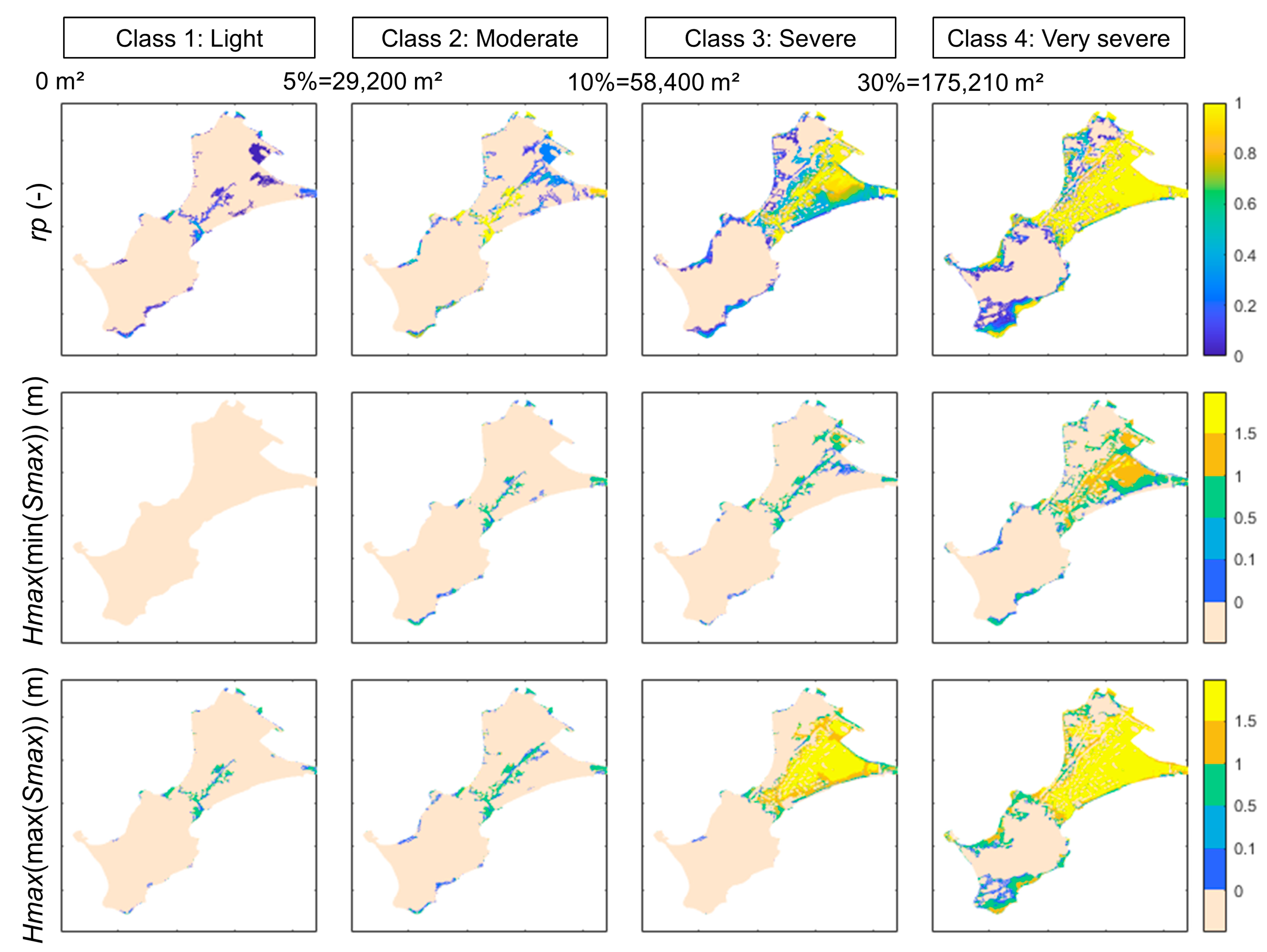
3.2.1. Flood Intensity and Spatial Flood Patterns

Here, we provide examples of statistical analysis of Smax and Hmax of use for knowledge of physical processes (e.g., water pathways), risk prevention (e.g., preferential flooded areas), and risk preparation (e.g., preferential routes and shelters for emergency operations).

First, the integrated map of rp values (Figure 7b) allows a preliminary identification of the preferential water pathways and of the areas which may have the largest chances to be flooded (the chance is as large as the rp value). We can distinguish two preferential water pathways (largest rp values), which are the root of the tombolo and the area close to the cemetery (location: Figure 3a) together with the road starting from the cemetery and running northeast. It should be noted that rp is calculated without considering the occurrence probability of each scenario. This means that rp can only be considered as an indicator of “chance of flooding”, but it does not quantify the flooding probability per se as rigorously as in a full probabilistic analysis. One key to doing so is to assess the responses of a large set of stochastically generated forcing conditions. Several difficulties exist, however, namely accounting for the dependence of forcings, randomly generating events of low probability, and rapidly predicting flood maps. Rohmer et al. [22] provided an example of flooding probability using a scalar flooding indicator. More advanced metamodelling techniques like those of Lopez-Lopera et al. [16], however, must be used to extend this analysis to maps of flooding probability (i.e., assess coastal flood hazard for risk prevention).

Keeping in mind this limitation, such types of analyses can be refined by analysing the flooded surface and water depth for different classes of flood intensity. Within the RISCOPE project, classes in the flooded area (m²) have been set up for the needs of the FEWS. The thresholds between the classes have been defined (in concertation with final users) based on a progressive increase in the proportion of flooded area, (0, 5, 10, and 30% of the study area, i.e., the blue area in Figure 1b), leading to null light, moderate, severe, and very severe flood intensity, respectively. In this classification, the past observed Johanna flood event falls in the “severe” class. Similarly to Figure 7b, which shows the ratio rp between the number of scenarios in which the pixel is flooded and the total number of scenarios for each pixel and accounting for all the scenarios, we can estimate rp specifically for each of the four severity classes, accounting only for the subset of scenarios falling in each class (Figure 8). These rp plots allow refining the preliminary analysis of the preferential water pathways and flooded areas depending on flood intensity. For light and moderate flood events (Classes 1 and 2), the two preferential water pathways are the root of the tombolo and the area close to the cemetery (location: Figure 3a) together with the road starting from the cemetery. Indeed, in case of light flood, the waves overtop the coastal defences in front of the cemetery (location: Figure 3a, confirmed by local in situ observations), and then the water propagates via the road network (road location: Figure 3a). As the water volume is small, the propagation does not extend too much. For the severe floods (class 3), additional areas with high rp values are the sports area (location: Figure 3a) and its surroundings. Indeed, in this case, there is much more wave overtopping in front of the sports area, and, as this terrain is a lowland (topographic depression), all the water overtopping the seafront converges toward these zones. Such information may be of use in supporting crisis preparation by indicating the preferential routes for emergency operations but also by highlighting the safest areas (rp = 0) to support/validate the selection of shelters and the location of the crisis management unit.

The CFMDG dataset can also be used to analyse the maximum water depth (reached over each simulation in each location) depending on the classes: Figure 8 (second and third rows) shows the Hmax maps corresponding to the simulations that led to the minimum and maximum Smax values within each Smax class. The colour scale of Hmax is designed based on the needs of local users (see [10]; for instance, the threshold of 0.1 m is important for emergency services). Such information, associated with the Smax class, may be of use during crisis management to quickly identify areas potentially exceeding this threshold and also areas subject to the greatest water depth. For the present Smax classification, we can see that Class 1 covers events leading to almost no flood (first column, second row: a single inland pixel is flooded, and Hmax < 0.1 m), to a more significant flood extent (but still limited), and to Hmax values locally reaching the class “0.5 to 1 m”. We may notice that the flood extent of the class (first column, first row) differs from the extent of the most penalizing event (first column, third row). Indeed, we should keep in mind that the rp maps integrate a variety of scenarios, which induce different flooded locations. Considering Class 2, the Hmax maps corresponding to the events minimising and maximising the Smax value indicate a larger extent (still concentrated in the cemetery and neighbouring roads) of Hmax values falling in the range “0.5 to 1 m”. For Classes 3 and 4, significant water depths are reached. Most of the flooded areas are now subject to water depths greater than 0.1 m, while large areas are subject to several tens of centimetres, exceeding 1.5 m in some cases.

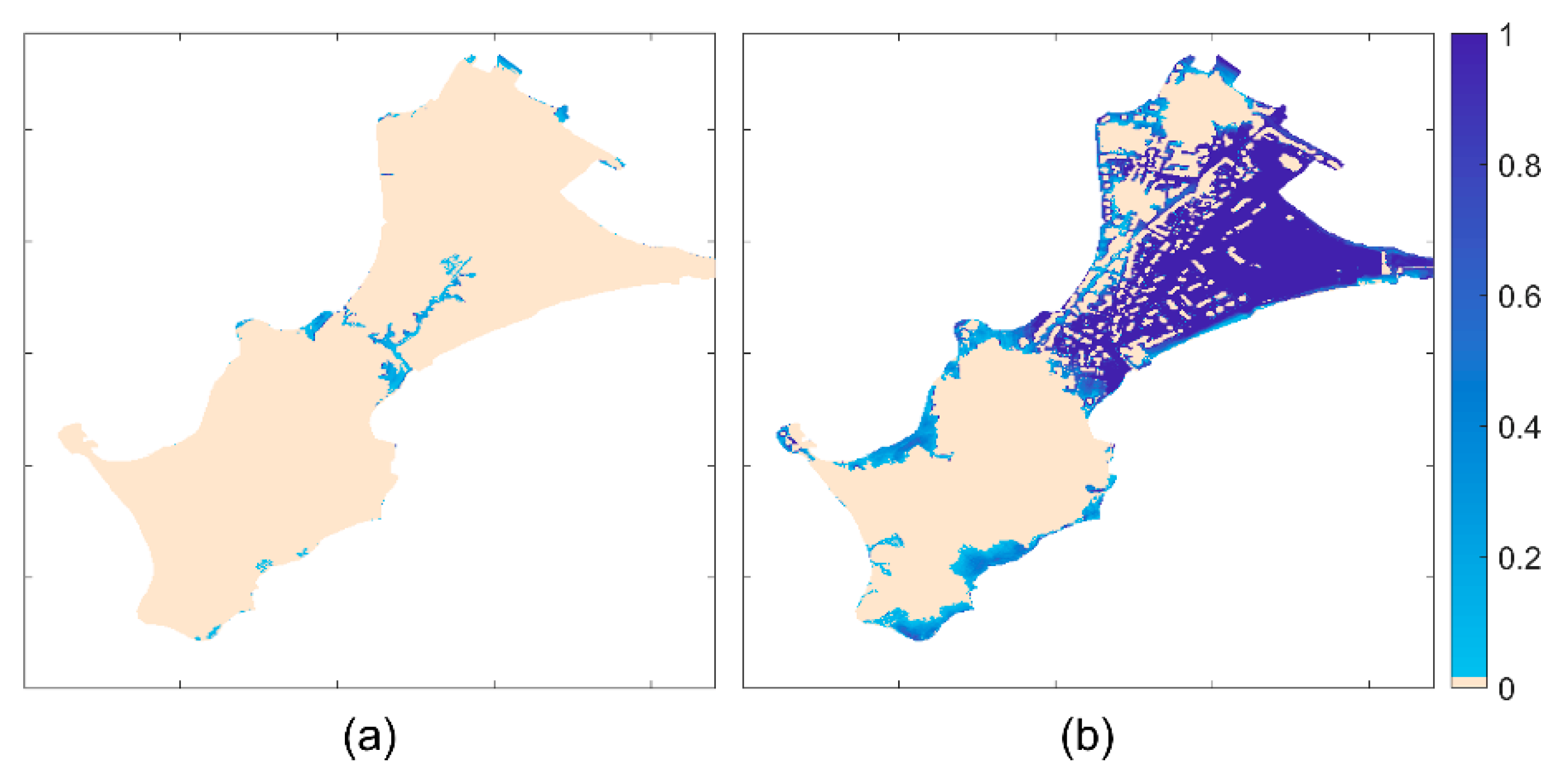
3.2.2. Present and Future Effect of Past Hydro-Meteorological Events

Past flood events are often used as a reference for flood hazard assessment. However, the first issue when investigating historical flood events is to have access to the forcing conditions corresponding to these events. The present dataset allows access to these forcing conditions for the following nine known past flood events (five major and four minor): 02/02/1904 04:00 (sc110), 09/01/1924 05:30 (sc95), 26/02/1978 05:30 (sc96), 10/01/2001 03:40 (sc98), 07/02/2001 15:20 (sc106), 27/10/2004 15:20 (sc99), 10/03/2008 05:20 (sc100 and sc116), 10/02/2009 04:00 (sc101), 28/02/2010 03:10 (sc108). For the 10/03/2008 event, there are two scenarios: sc100 is extracted from the continuous forcing conditions over the 1900–2016 period built by Idier et al. [3], while for sc116, the storm surge component is estimated based on the simulations performed by Le Roy et al. [2].

The CFMDG dataset can be used to estimate the effect that such past forcing conditions would have on the territory. We should keep in mind that the territory, topography, and coastal defences may have significantly changed such that the same forcing conditions (X) may lead to different flooding (Y). This is the case for the territory of Gâvres [3], where, for the same forcing conditions, the flood (obtained with our modelling approach for a digital elevation model and coastal defence configuration representative of 2018) should be smaller than the past observed floods (see [3]). Indeed, Figure 6a (sc95 to sc116, Group S1) illustrates that these past forcing conditions would lead to smaller flood intensity, with events leading to no flooding or light flooding (from sc = 95 to 116, the maximal value of Smax is 16,839 m² for sc = 116). This is even better illustrated when focussing on the most recent major flood event, which occurred in 2008 (Johanna storm, forcing conditions corresponding to sc116): the present topography and coastal defences (DEM2018, Figure 9a) appear much more protective against floods than those of 2008 (DEM2008, Figure 3a).

The CFMDG dataset also includes scenarios of sea level rise (the present mean sea level–NM–is 0.532 m in the IGN datum, while the NM values of the dataset range from 0.3 to ~2 m) and thus may provide knowledge on future floods and hazards. Among the scenarios of variations around past real forcing conditions, scenario N° 118 corresponds to scenario N° 116 (Johanna, best estimate), but with a sea level rise of +1 m (i.e., NM (sc = 118) = NM (sc = 116) + 1). Figure 9 illustrates the significant effect that such a sea level rise of 1 m would have if the Johanna forcing conditions occurred again in the future, assuming an unchanged DEM (DEM2018). Such types of figures/information are also useful in raising local risk awareness and triggering risk mitigation and adaptation.

3.3. Examples of Use of the CFMDG Dataset for Methods Development and Forecast

The dataset introduced here is directly of use to develop, test and compare metamodelling techniques, especially regarding problems of functional input (i.e., time-varying forcing conditions) and scalar (i.e., a single value) or functional (i.e., time and/or space varying) outputs (in general).

One part of this dataset has, for instance, already been used to develop and train metamodels aiming at predicting either the flooded area (Smax) or maps of water depths inland (Hmax). These developments rely on Gaussian processes (GP) and allow prediction in a few seconds and a few minutes, respectively, instead of the 3 days of computations on 48 cores.

First, a GP-based metamodelling approach was developed by Betancourt [14] to predict Smax. To reduce both the memory and the processing requirements of the metamodel, B-spline [23] and principal component analysis (PCA, [24]) dimension reduction techniques were used, as was thoroughly explained in [19]. In many studies, the structural characteristics of the metamodels are chosen beforehand (e.g., PCA decomposition in [25], B-spline decomposition in [26], the partial least square decomposition in [27]) without a specific sensitivity analysis or benchmarking. In the work of Betancourt [14], the ant-colony-based optimisation algorithm named “ACO-Gp” is used (see further technical details in [15,28]). It allows for the optimisation of the prediction quality while efficiently exploring the space of potential metamodel configurations, such as the set of inputs to use for prediction and the type of kernel function of the model. Implementations for functional input GP-based metamodelling and structural optimisation supported on ACO-Gp are available through the funGp R package [15], freely accessible from CRAN at https://cran.r-project.org/package=funGp, accessed on 13 June 2023 and GitHub at https://github.com/djbetancourt-gh/funGp, accessed on 13 June 2023. Betancourt et al. [15] and Idier et al. [10] used the above approach and a subset of 174 scenarios (sc1 to sc117, sc119 to sc132, sc139 to sc178, sc180 to sc182; Table 2) to train and cross-validate a metamodel predicting Smax. The obtained metamodel exhibits high predictive skills with a coefficient of determination value, denoted Q² (in a leave-one-out LOO cross-validation procedure) of 0.958, but with some weaknesses to properly detect the zero cases (no flood).

Regarding the water depth inland, López-Lopera et al. [16] developed a metamodelling technique that provided the ability to account not only for the functional inputs (time series) but also for functional (spatial) outputs. Implementations in both Python and R are freely available at https://github.com/anfelopera/spatfGPs, accessed on 13 June 2023. They applied this method to predict Hmax in each inland point at Gâvres using a subset of 131 scenarios (sc1 to sc118 and sc120 to sc132) and different subsets of the inland points (103 and 1003 points) to train the metamodel. Considering for instance the predictions for the 131 LOO tests and the 103 points subset, they resulted in Q² and CA (coverage accuracy of the predictive intervals defined at ±2 standard deviation) median values of approximately 95.8% and 99%, respectively (when analysing the prediction on the 103 points). The results appearing to be promising, this is finally a subset of 174 scenarios (sc1 to sc117, sc119 to sc132, sc139 to sc178, sc180 to sc182) which was used to train the metamodel before its implementation in a FEWS prototype [10].

As highlighted in [10,15,16], both metamodels exhibit lower predictive power in the discrimination between flood (Smax > 0, Hmax > 0) and no flood (Smax = 0, Hmax = 0). To limit the errors in the FEWS prototype, a pragmatic approach was used in [10] by combining these metamodels with another one [29], fundamentally different, which uses scalar inputs and focuses on the water volume entering inland in 20 min time spans (and thus does not provide any explicit information on the flooded area or the water depth inland). Although operative in the RISCOPE application case, this approach could be replaced by alternative techniques of wider theoretical ground. One way to improve the metamodel prediction relying on the GP-based metamodels close to 0 is to increase the number of learning scenarios providing no flood (Y = 0). This strategy was tested by adding 40 non-flood event scenarios (sc183 to sc222) to the existing 174 scenarios used in the learning dataset, but no significant improvement was found. A more promising perspective of improvement is to use refinements of GP models that are tailored for modelling positive functions and may provide more accurate metamodel predictions of output values close to 0. Two examples of these refinements are truncated GP models [30] and constrained GP models [31,32]. If metamodels other than GPs are considered, then it would also be possible to have an interaction between the classification problem of zero outputs and the regression problem of non-zero outputs (as tested in [29]). By making the present dataset available, we expect and facilitate future investigation/progress around this topic.

4. Discussion

4.1. Use of the Dataset for Method Development and Forecasting

For the flood forecast, the added value of the present dataset is twofold: (1) local forecast to the Gâvres site (i.e., site-specific, as in [10]); (2) development of forecasting methods. As highlighted in [10], the need of the users is to know if there will be a flood event or not, and if so, of which intensity. The need of spatial maps only appears in the second phase. Such maps allow better predicting where there will be a flood and thus support risk prevention or crisis preparation and management actions. Thus, an alternative to prototypes that are fully based on metamodels (as in [10]), is to estimate the primary information of interest (flooded surface based on a metamodel predicting Smax) and then to use the associated rp maps (see, e.g., Figure 8 for the flood intensity classes defined in Section 4.1) to estimate the envelope of potential flooded zones (map) corresponding to any Smax classes defined by the user of the dataset depending on its specific need. In addition, the FEWS prototype developed by Idier et al. [10] is determinist (i.e., metamodel simulations are performed for single meteo-oceanic forcing condition X). The next step would be to use such a metamodelling approach (fast running) to move from deterministic to probabilistic forecast using as inputs the outputs of Ensemble meteo-oceanic prediction systems.

A second approach for forecasting floods is to rely on a lookup table method. Such a method consists, for each desired input condition (e.g., forecasted 6 h time series for the next tide), of identifying in a pre-existing computed database (here, the CFMDG dataset) which existing scenario (scenarios) is (are) the closest to the desired conditions, i.e., based on a distance (or similarity) measure in the input domain of variation. This approach has, for instance, been used in many applications when the inputs and outputs are treated as scalar continuous variables; for instance, for transforming wave characteristics from deep to shallow water conditions (see, e.g., [33] along the Long Beach peninsula in the US) or for fast prediction of a hurricane-induced surge in coastal Mississippi [34]. When the inputs are functions (e.g., time series such as in the Gâvres case), more advanced distance functions must be defined (see [15] and references therein). Thus, the present dataset may be of use in developing and testing methods to compute the distances in the X space (when X is made of time series) and the uncertainty associated with the selected scenario of the dataset. It may also be used to develop any other alternative methods requiring a learning dataset.

4.2. The limits of a Steady Topo-Bathymetry

In addition to hydro-meteorological forcing, floods are also related to topo-bathymetry and especially to the coastal defences in place. The present dataset has been built for a constant topo-bathymetry (and coastal defences) representative of the 2018 winter. In case of significant change in this topo-bathymetry and coastal defences in the future, the present dataset for local applied studies aiming at investigating coastal hazards should be used with caution. For instance, based on the analyses of the DEM differences, the user may estimate if the new configuration should lead to more (or less) flooding for the same hydro-meteorological forcing conditions and thus should be able to stress if the use of the present dataset for such a new site configuration should under- or over-predict the flooding.

4.3. Recommendations for Generating Similar Datasets in Other Locations

As guidelines to support the development of similar training datasets for flood investigations in another location, our recommendations are as follows. A preliminary step is to identify if flood events occurred in the past, and, in this case, if they result mainly from overflow or wave overtopping processes. This will support the choice of the numerical modelling approach. Then, the availability and quality of local topo-bathymetric data (and coastal defences) should be analysed. In case of too-low vertical precision (e.g., errors larger than 10 cm), data should be acquired to obtain a precise enough DEM. Then, following the method described in Figure 2, the locations in which forcing conditions are needed should be identified. At these locations, a long enough set of past forcing conditions (e.g., 10 years) should be built. It can be built based on observations (if available) or reanalysis. Then, a hydrodynamic model should be set up and validated in front of quantitative or qualitative data. It is at this stage that scenarios must be designed. Depending on the environment (macro-tidal/micro-tidal) and the modelling strategy, the scenarios can be time-varying (as in the present manuscript) or steady (as in [9]). When the number of affordable scenarios is limited in comparison to the number of drivers, we recommend combining past events and fictive events designed based on extreme value analysis. When this number is large in comparison to the number of main drivers, the design may rely on more pragmatic approaches which do not require skills in extreme value analysis (see, e.g., [9], which considered a regular discretisation of the driver space but applied filtering based on the analysis of the distribution of these drivers in the past). Depending on the specific use of the dataset, attention should also be paid to including cases in which no flood is expected (such scenarios are needed both for metamodel development and for lookup table approaches). Then, the hydrodynamic simulations can be performed for scenarios including specific past conditions and fictive conditions (and, when needed, scenarios in which no floods are expected). Finally, as in the present dataset, the model outputs may be post-processed to ease the dataset diffusion (light files) and the analysis of the final dataset.

One recommendation we may provide when the total number of simulations is imposed would be to build the dataset iteratively, especially when the aim is to develop metamodels for fast prediction. This is particularly interesting when using kriging metamodelling techniques, as they provide uncertainty information in the prediction such that in the next iteration, we may want to add additional scenarios in areas of high interest and large prediction uncertainty (see, e.g., [6] for an example of such iterative sampling).

5. Conclusions

The CFMDG dataset compiles a set of 250 scenarios of forcing conditions and induced flooded surfaces (Smax) and water depths inland (Hmax), obtained via hydrodynamic modelling and post-processing. Each scenario is a combination of 6 h long time series of the different forcing variables, centred on high tide. The dataset covers a wide range of coastal flood intensities. Several examples of past and future potential use of this dataset have been provided, from direct analysis for site-specific knowledge (processes, hazard, prevention) to method development (metamodels, forecast). We hope that making this dataset publicly accessible will trigger further methodological developments in machine-learning/metamodel-based techniques to support flood prediction.

The procedure we used was adapted to the characteristics of the site (e.g., macro-tidal, complex seafronts) and the modelling choices (here, a quasi-3D modelling accounting for the nearshore and inland dynamics, including wave overtopping processes). In the case of micro-tidal sites—and depending on the selected modelling approach—while the main steps remain valid, the design of the scenarios may be adapted (as illustrated in this paper, it may be indeed simpler).

In terms of practice, especially when the number of simulations is limited, we recommend building such datasets iteratively to ensure that the final dataset is as optimal as possible regarding the initial need.

For specific studies related to the site of Gâvres, the dataset presents the limit to have been built for topo-bathymetry and coastal defences representative of the 2018 situation, restricting the validity domain. Generating such a dataset for different digital elevation models may be one perspective which is also relevant for the development of metamodels treating the DEM as an input.

References

1. Wolf, J. Coastal Flooding: Impacts of Coupled Wave–Surge–Tide Models. Nat. Hazards 2009, 49, 241–260. [Google Scholar] [CrossRef] [Green Version]
2. Le Roy, S.; Pedreros, R.; André, C.; Paris, F.; Lecacheux, S.; Marche, F.; Vinchon, C. Coastal Flooding of Urban Areas by Overtopping: Dynamic Modelling Application to the Johanna Storm (2008) in Gâvres (France). Nat. Hazards Earth Syst. Sci. 2015, 15, 2497–2510. [Google Scholar] [CrossRef] [Green Version]
3. Idier, D.; Rohmer, J.; Pedreros, R.; Le Roy, S.; Lambert, J.; Louisor, J.; Le Cozannet, G.; Le Cornec, E. Coastal Flood: A Composite Method for Past Events Characterisation Providing Insights in Past, Present and Future Hazards—Joining Historical, Statistical and Modelling Approaches. Nat. Hazards 2020, 101, 465–501. [Google Scholar] [CrossRef] [Green Version]
4. Idier, D.; Pedreros, R.; Rohmer, J.; Le Cozannet, G. The Effect of Stochasticity of Waves on Coastal Flood and Its Variations with Sea-Level Rise. J. Mar. Sci. Eng. 2020, 8, 798. [Google Scholar] [CrossRef]
5. Gao, J.; Ma, X.; Zang, J.; Dong, G.; Ma, X.; Zhu, Y.; Zhou, L. Numerical Investigation of Harbor Oscillations Induced by Focused Transient Wave Groups. Coast. Eng. 2020, 158, 103670. [Google Scholar] [CrossRef]
6. Rohmer, J.; Idier, D. A Meta-Modelling Strategy to Identify the Critical Offshore Conditions for Coastal Flooding. Nat. Hazards Earth Syst. Sci. 2012, 12, 2943–2955. [Google Scholar] [CrossRef]
7. Rohmer, J.; Lecacheux, S.; Pedreros, R.; Quetelard, H.; Bonnardot, F.; Idier, D. Dynamic Parameter Sensitivity in Numerical Modelling of Cyclone-Induced Waves: A Multi-Look Approach Using Advanced Meta-Modelling Techniques. Nat. Hazards 2016, 84, 1765–1792. [Google Scholar] [CrossRef]
8. Jia, G.; Taflanidis, A.A. Kriging Metamodeling for Approximation of High-Dimensional Wave and Surge Responses in Real-Time Storm/Hurricane Risk Assessment. Comput. Methods Appl. Mech. Eng. 2013, 261–262, 24–38. [Google Scholar] [CrossRef]
9. Chondros, M.; Metallinos, A.; Papadimitriou, A.; Memos, C.; Tsoukala, V. A Coastal Flood Early-Warning System Based on Offshore Sea State Forecasts and Artificial Neural Networks. J. Mar. Sci. Eng. 2021, 9, 1272. [Google Scholar] [CrossRef]
10. Idier, D.; Aurouet, A.; Bachoc, F.; Baills, A.; Betancourt, J.; Gamboa, F.; Klein, T.; López-Lopera, A.F.; Pedreros, R.; Rohmer, J.; et al. A User-Oriented Local Coastal Flooding Early Warning System Using Metamodelling Techniques. J. Mar. Sci. Eng. 2021, 9, 1191. [Google Scholar] [CrossRef]
11. Ardhuin, F.; Rogers, W.E.; Babanin, A.V.; Filipot, J.; Magne, R.; Roland, A.; Van der Westhuysen, A.; Queffelou, P.; Lefevre, J.; Aouf, L.; et al. Semiempirical Dissipation Source Functions for Ocean Waves. Part I: Definition, Calibration, and Validation. J. Phys. Oceanogr. 2010, 40, 917–941. [Google Scholar] [CrossRef] [Green Version]
12. Zijlema, M.; Stelling, G.; Smit, P. SWASH: An Operational Public Domain Code for Simulating Wave Fields and Rapidly Varied Flows in Coastal Waters. Coast. Eng. 2011, 58, 992–1012. [Google Scholar] [CrossRef]
13. Idier, D.; Rohmer, J.; Pedreros, R.; Le Roy, S.; Betancourt, J. CFMDG: A Coastal Flood Modelling Dataset in Gâvres (France) to Support Risk Prevention and Metamodels Development. 2023. Available online: https://www.fatcat.wiki/release/co4mxdvhvzbtbiqhujwkri55tm (accessed on 13 June 2023).
14. Betancourt, J.D. Functional-Input Metamodeling: An Application to Coastal Flood Early Warning. Ph.D. Thesis, Université Paul Sabatier—Toulouse III, Toulouse, France, 2020. [Google Scholar]
15. Betancourt, J.; Bachoc, F.; Klein, T.; Idier, D.; Rohmer, J.; Deville, Y. FunGp: An R Package for Gaussian Process Regression with Scalar and Functional Inputs; Archive Ouverte HAL: Lyon, France, 2022. [Google Scholar]
16. López-Lopera, A.F.; Idier, D.; Rohmer, J.; Bachoc, F. Multioutput Gaussian Processes with Functional Data: A Study on Coastal Flood Hazard Assessment. Reliab. Eng. Syst. Saf. 2022, 218, 108139. [Google Scholar] [CrossRef]
17. Pedreros, R.; Idier, D.; Roy, S.L.; David, A.; Schaeffer, C.; Durand, J.; Desmazes, F. Infragravity waves in a complex macro-tidal environment: High frequency hydrodynamic measurements and modelling. Global Coastal Issues of 2020. J. Coast. Res. 2020, 95, 1235–1239. [Google Scholar] [CrossRef]
18. Lyard, F.H.; Allain, D.J.; Cancet, M.; Carrère, L.; Picot, N. FES2014 Global Ocean Tide Atlas: Design and Performance. Ocean Sci. 2021, 17, 615–649. [Google Scholar] [CrossRef]
19. Betancourt, J.; Bachoc, F.; Klein, T.; Idier, D.; Pedreros, R.; Rohmer, J. Gaussian Process Metamodeling of Functional-Input Code for Coastal Flood Hazard Assessment. Reliab. Eng. Syst. Saf. 2020, 198, 106870. [Google Scholar] [CrossRef] [Green Version]
20. Gouldby, B.; Méndez, F.J.; Guanche, Y.; Rueda, A.; Mínguez, R. A Methodology for Deriving Extreme Nearshore Sea Conditions for Structural Design and Flood Risk Analysis. Coast. Eng. 2014, 88, 15–26. [Google Scholar] [CrossRef] [Green Version]
21. Tharwat, A. Linear vs. Quadratic Discriminant Analysis Classifier: A Tutorial. Int. J. Appl. Pattern Recognit. 2016, 3, 145–180. [Google Scholar] [CrossRef]
22. Rohmer, J.; Idier, D.; Thieblemont, R.; Le Cozannet, G.; Bachoc, F. Partitioning the Contributions of Dependent Offshore Forcing Conditions in the Probabilistic Assessment of Future Coastal Flooding. Nat. Hazards Earth Syst. Sci. 2022, 22, 3167–3182. [Google Scholar] [CrossRef]
23. De Boor, C. A Practical Guide to Splines; Springer: New York, NY, USA, 1978; ISBN 978-0-38795-366-3. [Google Scholar]
24. Jolliffe, I.T. Principal Component Analysis, 2nd ed.; Springer: New York, NY, USA; Berlin/Heidelberg, Germany, 2002; ISBN 978-0-38795-442-4. [Google Scholar]
25. Antoniadis, A.; Helbert, C.; Prieur, C.; Viry, L. Spatio-Temporal Metamodeling for West African Monsoon. Environmetrics 2012, 23, 24–36. [Google Scholar] [CrossRef] [Green Version]
26. Muehlenstaedt, T.; Fruth, J.; Roustant, O. Computer Experiments with Functional Inputs and Scalar Outputs by a Norm-Based Approach. Stat. Comput. 2017, 27, 1083–1097. [Google Scholar] [CrossRef] [Green Version]
27. Nanty, S.; Helbert, C.; Marrel, A.; Pérot, N.; Prieur, C. Sampling, Metamodeling, and Sensitivity Analysis of Numerical Simulators with Functional Stochastic Inputs. SIAMASA J. Uncertain. Quantif. 2016, 4, 636–659. [Google Scholar] [CrossRef]
28. Betancourt, J.D.; Bachoc, F.; Klein, T.; Gamboa, F. Ant Colony Based Model Selection for Functional-Input Gaussian Process Regression; Research Report D3.b; Institut de Mathématiques de Toulouse & Institut Universitaire de France, UMR 5219, Université de Toulouse, CNRS, UPS IMT; HAL: Lyon, France, 2020; Available online: https://hal-enac.archives-ouvertes.fr/hal-02532713 (accessed on 13 June 2023).
29. Rohmer, J.; Idier, D.; Pedreros, R. A Nuanced Quantile Random Forest Approach for Fast Prediction of a Stochastic Marine Flooding Simulator Applied to a Macrotidal Coastal Site. Stoch. Environ. Res. Risk Assess. 2020, 34, 867–890. [Google Scholar] [CrossRef]
30. Stein, M.L. Prediction and Inference for Truncated Spatial Data. J. Comput. Graph. Stat. 1992, 1, 91–110. [Google Scholar] [CrossRef]
31. López-Lopera, A.F.; Bachoc, F.; Durrande, N.; Roustant, O. Finite-Dimensional Gaussian Approximation with Linear Inequality Constraints. SIAMASA J. Uncertain. Quantif. 2018, 6, 1224–1255. [Google Scholar] [CrossRef]
32. Vanhatalo, J.; Vehtari, A. Sparse Log Gaussian Processes via MCMC for Spatial Epidemiology. In Proceedings of the Gaussian Processes in Practice, PMLR, Bletchley Park, UK, 2–13 June 2006; pp. 73–89. [Google Scholar]
33. Ruggiero, P.; List, J.; Hanes, D.; Eshleman, J. Probabilistic Shoreline Change Modeling. In Coastal Engineering 2006; World Scientific Publishing Company: Singapore, 2007; pp. 3417–3429. ISBN 978-9-81270-636-2. [Google Scholar]
34. Das, H.S.; Jung, H.; Ebersole, B.; Wamsley, T.; Whalin, R.W. An Efficient Storm Surge Forecasting Tool for Coastal Mississippi. Coast. Eng. Proc. 2010, 32, 21. [Google Scholar] [CrossRef] [Green Version]
35. Rohmer, J.; Cozannet, G.L. Dominance of the Mean Sea Level in the High-Percentile Sea Levels Time Evolution with Respect to Large-Scale Climate Variability: A Bayesian Statistical Approach. Environ. Res. Lett. 2019, 14, 014008. [Google Scholar] [CrossRef]
36. Santamaría-Gómez, A.; Gravelle, M.; Dangendorf, S.; Marcos, M.; Spada, G.; Wöppelmann, G. Uncertainty of the 20th Century Sea-Level Rise Due to Vertical Land Motion Errors. Earth Planet. Sci. Lett. 2017, 473, 24–32. [Google Scholar] [CrossRef]
37. Compo, G.P.; Whitaker, J.S.; Sardeshmukh, P.D.; Allan, R.J.; McColl, C.; Yin, X.; Giese, B.S.; Vose, R.S.; Matsui, N.; Ashcroft, L.; et al. NOAA/CIRES Twentieth Century Global Reanalysis Version 2c 2015, 11.170 Tbytes. Available online: https://rda.ucar.edu/datasets/ds131.2/ (accessed on 13 June 2023).
38. Dee, D.P.; Balmaseda, M.; Balsamo, G.; Engelen, R.; Simmons, A.J.; Thépaut, J.-N. Toward a Consistent Reanalysis of the Cli-mate System. Bull. Am. Meteorol. Soc. 2014, 95, 1235–1248. [Google Scholar] [CrossRef] [Green Version]
39. Muller, H.; Pineau-Guillou, L.; Idier, D.; Ardhuin, F. Atmospheric Storm Surge Modeling Methodology along the French (Atlantic and English Channel) Coast. Ocean Dyn. 2014, 64, 1671–1692. [Google Scholar] [CrossRef] [Green Version]
40. Bertin, X.; Prouteau, E.; Letetrel, C. A Significant Increase in Wave Height in the North Atlantic Ocean over the 20th Century. Glob. Planet. Change 2013, 106, 77–83. [Google Scholar] [CrossRef]
41. Charles, E.; Idier, D.; Thiebot, J.; Le Cozannet, G.; Pedreros, R.; Ardhuin, F.; Planton, S. Present Wave Climate in the Bay of Biscay: Spatiotemporal Variability and Trends from 1958 to 2001. J. Clim. 2012, 25, 2020–2039. [Google Scholar] [CrossRef]
42. Boudière, E.; Maisondieu, C.; Ardhuin, F.; Accensi, M.; Pineau-Guillou, L.; Lepesqueur, J. A Suitable Metocean Hindcast Data-base for the Design of Marine Energy Converters. Int. J. Mar. Energy 2013, 3–4, e40–e52. [Google Scholar] [CrossRef] [Green Version]
Figure 1. Location of input (scenarios) and output (post-processed model outputs) datasets. (a) Location of input data and computational domain of the numerical models WW3 and SWASH (coordinates in WGS84, °). The coordinates of the input variables are: (−3.36° E, 47.68° N) for ξ, with ξ = NM + T + S; (−3.48° E, 47.56° N) for Hs, Tp and Dp; (−3.44° E, 47.62° N) for U and DU. (b) Location of output data (coordinates projected in the local system Lambert 93, m), overlapped on ortho-photographies provided by the French National Institute of Geographic and Forest Information (IGN).
Jmse 11 01314 g001
Figure 2. Method used to build the CFMDG dataset. Except for Step 6, all the illustrations are extracted from figures presented and described in more detail in Section 2 and Section 3. The grey arrows indicate the main required external data. B1, B2, and B3 refer to Blocks 1, 2, and 3, respectively.
Jmse 11 01314 g002
Figure 3. Modelling chain validation. (a) Coastal flood event of 10 March 2008 (Johanna storm; observed flooded houses and maximum modelled water depth in each flooded pixel—according to the model results—with a transparency applied to the model outputs to better see the ground and land use), localisation of the pressure sensor, key information (road network in grey, cemetery and sports area location), and area of preferential wave overtopping (in the general case, indicated by arrows); (b) observed and modelled significant wave height (Hm0; for entire band and infragravity–IG band) at the pressure sensor location (see panel (a)) and for the following three 17 min long bursts (each at 2 Hz frequency): B1: 29/11/2018 04:30, B2: 17/11/2018 23:57, B3: 04/03/2019 05:14. Panel (b) adapted from [17], reproduced and modified with permission from the Coastal Education and Research Foundation, Inc.
Jmse 11 01314 g003
Figure 4. Hydro-meteorological database of [3] over the period from 1900–2016: time series of the relative mean sea level (NM) and distribution of the other hydro-meteorological variables: tide (T), surge (S), significant wave height (Hs), peak period (Tp), peak direction (Dp), wind velocity (U), and wind direction (DU).
Jmse 11 01314 g004
Figure 5. Overview of the X dataset: (a) type of scenario (S1 to S5, see Table 2) for each scenario, (b) time series of the forcing conditions for each scenario (250 curves for the 250 scenarios) from 3 h before high tide (H.T.) to 3 h after high tide (colours are used to better distinguish the time series, each scenario has the same colour in each subpanel).
Jmse 11 01314 g005
Figure 6. Overview of the Y dataset: (a) Y dataset/flooded area (Smax, m2) with the scenario numbering described in Table 2. (b) Y dataset/maximum water depth (Hmax, m) per inland pixel for each scenario (in the same order as on panel (a)).
Jmse 11 01314 g006
Figure 7. Integrated Smax and Hmax view: (a) distribution of Smax in terms of class, with the classes defined by the ratio rS between the flooded area (Smax) and the total study area (Stot); (b) for each pixel, ratio (rp) of the number of scenarios where the pixel is flooded to the total number of simulations.
Jmse 11 01314 g007
Figure 8. Maps of flooded pixels and Hmax values for each (pre-defined) Smax class, i.e., accounting only for the subset of scenarios falling in each class. First row: rp values (as in Figure 7). Second and third rows: Hmax values corresponding to the scenarios having led to the minimal and maximal values of Smax (within the Smax class). To be noted: min (Smax) for class 1 equals 9 m2 such that only a single point (pixel) is flooded (at the southwest), not visible on the figure.
Jmse 11 01314 g008
Figure 9. Simulated maximal inland water depth (Hmax, m) induced by the forcing conditions of the Johanna event (a) without (sc116) and (b) with (sc118) a sea level rise of +1 m.
Jmse 11 01314 g009