Optimal Route Generation and Route-Following Control for Autonomous Vessel

Abstract

In this study, basic research was conducted regarding the era of autonomous vessels and artificial intelligence (deep learning, big data, etc.). When a vessel is navigating autonomously, it must determine the optimal route by itself and accurately follow the designated route using route-following control technology. First, the optimal route should be generated in a manner that ensures safety and reduces fuel consumption by the vessel. To satisfy safety requirements, sea depth, under-keel clearance, and navigation charts are used; algorithms capable of determining and shortening the distance of travel and removing unnecessary waypoints are used to satisfy the requirements for reducing fuel consumption. In this study, a reinforcement-learning algorithm-based machine learning technique was used to generate an optimal route while satisfying these two sets of requirements. Second, when an optimal route is generated, the vessel must have a route-following controller that can accurately follow the set route without deviation. To accurately follow the route, a velocity-type fuzzy proportional–integral–derivative (PID) controller was established. This controller can prevent deviation from the route because overshoot rarely occurs, compared with a proportional derivative (PD) controller. Additionally, because the change in rudder angle is smooth, energy loss by the vessel can be reduced. Here, a method for determining the presence of environmental disturbance using the characteristics of the Kalman filter innovation process and estimating environmental disturbance with a fuzzy disturbance estimator is presented, which allows the route to be accurately maintained even under conditions involving environmental disturbance. The proposed approach can automatically set the vessel’s optimal route and accurately follow the route without human intervention, which is useful and can contribute to maritime safety and efficiency improvement.

1. Introduction

With the advent of the Fourth Industrial Revolution, interest and demand for autonomous ships are rapidly increasing [1,2,3]. In particular, beginning with the Maritime Unmanned Navigation through Intelligence in Networks (MUNIN) project, there has been considerable active development and research regarding autonomous ships [4,5]. The International Maritime Organization defines autonomous ships as maritime autonomous surface ships (MASS) and has established four degrees of ship autonomy in response to the era of autonomous ships [6,7]. To satisfy the criteria for constituting a fully autonomous ship, route determination and route-following control technology are required; several technical factors must also be addressed. First, the ship must be safely operated based on a comprehensive understanding of the marine environment and port information throughout the navigation process. Second, it must be possible to plan the route to minimize fuel consumption or navigation time. Finally, a control technology is needed to enable the vessel to accurately follow the designated route.

Most vessels are equipped with an Electronic Chart Display and Information System (ECDIS) based on electronic navigation charts [8,9]; thus, it is easy to obtain various components of information needed to determine the route. Therefore, the route can be determined using electronic navigation charts instead of paper charts, which were widely used in the past. Traditionally, the knowledge of experienced officers has been an important factor in determining the optimal route, but there is a limit to optimal route generation because of the ever-changing maritime environment. Previous studies regarding route generation focused on reducing the fuel consumption and sailing time of vessels using the $A^{*}$ and Dijkstra algorithms [10,11]. These algorithms consider collision avoidance on land and islands, but they do not consider the sea depth and relevant regulations with which the vessel must comply. To solve this problem, research on reinforcement learning-based route generation is being actively conducted.

This study was performed to generate an optimal route by considering collision prevention on land and islands, as well as sea depth and relevant regulations that vessels must follow. We included an algorithm to reduce fuel consumption by the vessel. To achieve the objective of this study, a reinforcement-learning algorithm was used as an optimal route generation algorithm. The reinforcement-learning algorithm learns in the direction of maximizing the reward and derives the optimal solution. Therefore, unlike the existing $A^{*}$ and Dijkstra algorithms, a more realistic and practical route can be generated because various surrounding environmental conditions can be considered for route generation.

Control technology is required to enable the vessel to accurately follow a route after it has been generated [12]. Proportional–derivative (PD)-type autopilot controllers, which have been widely used in the past, are implemented in most vessels because their performance and stability have been verified [13]. However, such autopilot controllers have poor performance with regard to rapid course alterations and large changes in heading angle. Additionally, the change in rudder angle is rough, which reduces the energy efficiency of the vessel.

To resolve these issues, previous studies have utilized fuzzy logic theory. The stability problem of the fuzzy controller, which was a problem at the time of its introduction, has been analyzed and resolved by several groups [14,15]; it is widely applied in actual plants [16,17]. The fuzzy controller can hold expert language information while responding to nonlinear plants because of its nonlinear characteristics. Additionally, because the fuzzy proportional–integral–derivative (PID) controller is controlled according to fuzzy logic rules, it has the ability to optimally generate PID coefficient values that satisfy the control rules [18,19]. Therefore, such fuzzy PID controllers can achieve faster course alterations with less route deviation because of large overshoot compared with PD controllers. The fuzzy PID controller designed in this study is regarded as a velocity fuzzy PID controller because it is an incrementally controlled controller.

However, despite the use of a fuzzy PID controller with excellent performance, real vessels are not able to accurately follow the designated route if external environmental disturbances, such as winds, ocean currents, and waves, are encountered [20,21]. Therefore, to prevent vessel deviation from the designated route because of environmental disturbance, additional thrust and rudder angle must be generated to respond to such changes. In this study, the characteristics of the Kalman filter’s innovation process were used to determine the existence of environmental disturbances, and a fuzzy disturbance estimator was introduced to estimate their magnitude.

Because the Kalman filter is a model-based state estimation theory, the estimation error between the actual state of the system and the filter estimation increases when an unknown input (environmental disturbance) is applied [22,23]. The difference between the actual state of the system and the filter estimation is regarded as the innovation process [24,25]. If the Kalman filter fails state estimation, the innovation will chatter with a constant DC component. This phenomenon can be used to determine the presence of environmental disturbances. After confirmation of their presence, the magnitudes of environmental disturbances are estimated using a fuzzy disturbance estimator. Additionally, modification of the estimated environmental disturbances into thrust and rudder angle, followed by their application in the form of additional control input, allows the vessel to accurately follow the designated route despite environmental disturbance.

If the proposed reinforcement learning-based optimal route generation algorithm is applied, it will be a useful algorithm that can guarantee the safety of vessels when applied in real situations. In addition, since it has the ability to estimate the magnitude of environmental disturbances in real time and control the vessel based on this, it has the advantage of maintaining a designated route without the intervention of an officer. The method proposed in this study will serve as a foundation for the era of autonomous vessel.

2. Related Work

2.1. Route Generation

Since reinforcement learning can generate an optimal route considering the surrounding environment of a vessel, research on the field of generating an optimal route for a vessel is being actively conducted.

Based on the Q-learning algorithm, there is a study that generates a vessel’s route by modeling the distance to the destination and a prohibited area [26], and a global route generation model for coastal vessels using the Deep Q-Network algorithm have been proposed [27]. And, there is also a study on route generation for unmanned vessels using the information provided by ECDIS and deep deterministic policy gradient (DDPG) algorithm [28]. In addition to these, studies on route generation for collision avoidance between vessels are also being conducted [29,30,31].

Through these related work, it was confirmed that reinforcement learning can determine the vessel’s route. Therefore, in this study, in order to enable a vessel to follow the route in a more realistic route, it is intended to generate an optimal route using reinforcement learning. As an algorithm, Q-learning, whose performance has been verified, was applied.

2.2. Route-Following Control

Route-following control is an essential techniques allowing vessels to maintain a designated route. In order to follow the route, studies have been conducted using line-of-sight (LOS) guidance systems that determine an LOS vector from the current vessel’s position to any one point between the next waypoint and use this LOS vector to control the heading angle [32,33,34]. In addition, for the purpose of controlling it, controllers such as PID, fuzzy PID, and neural network, etc., have been applied [35,36,37]. However, these studies demonstrated that the performance is excellent in a state where no environmental disturbances are applied. No matter how good the route-following controller used is, if the vessel is subjected to environmental disturbances, it will not be able to follow the reference input, and steady-state error occurs.

In order to solve this problem, research has been conducted on how to configure an RFO observer using LMI [38], integral state observers [39], and proportional–integral state observers [40,41] as methods for estimating the magnitude of environmental disturbances. In addition, a method of estimating environmental disturbance using an error between an actual system state and as estimated state by constructing a sliding mode type observer has been studied [42,43,44]. However, the above methods are complicated and difficult to develop mathematically, so there is a limit to the performance improvement of disturbance estimation. In addition, since it is a fixed structure and is designed for asymptotic performance in a steady state, it has a disadvantage that it cannot quickly cope with rapidly changing disturbances.

Therefore, in this study, a velocity-type fuzzy PID controller was applied as a controller to follow the vessel’s route. In addition, the magnitude of the environmental disturbance can be estimated through the fuzzy disturbance estimator, which is composed of a variable structure and can quickly cope with rapidly changing environmental disturbance.

3. Dynamic Vessel Model

3.1. Coordinate Systems

To model and analyze the vessel, a body-fixed coordinate system and an earth-fixed coordinate system are introduced, as shown in Figure 1. The body-fixed coordinate system, a coordinate system for the analysis of vessel motion, is attached to the body frame of the vessel; the earth-fixed coordinate system, a coordinate system for analyzing the position and angle of the vessel on the earth, is attached to the center of gravity [45].

The variables of a body-fixed coordinate system $x_B{y}_B{z}_B$ are composed of $\left(u, v, w, p, q, r\right)$, where $\left(u,v, w\right)$ are the surge, sway, and heave as linear velocities, respectively; $\left(p,q, r\right)$ are the roll, pitch, and yaw as angular velocities of the vessel, respectively. The variables of an earth-fixed coordinate system $O_E$ are composed of $\left(\mathrm{x}, y, z, \varphi , \theta , \psi \right)$, where $\left(\mathrm{x}, y, z\right)$ are the position coordinates in three dimensions; and $\left(\varphi , \theta , \psi \right)$ are the roll, pitch, and yaw (heading) angles of the vessel, respectively.

3.2. Vessel Equation of Motion

Generally, a vessel is represented by 6-degree-of-freedom (DOF) equations of motion, which consist of the linear and angular velocities on the three axis directions. However, because most vessels operate on the horizontal surface of the sea, the 6 DOF equations of motion can be simplified to 3 DOF equations of motion [46] if the following assumptions are made:

(1)

Roll, pitch, and heave motions of the vessel are negligible.

(2)

The shape of the vessel is symmetrical in the $x_B{z}_B$ plane.

(3)

The origin of the body-fixed coordinate system is located at the center of the vessel.

In this study, the model proposed by Blanke was used as the forward speed model; the model proposed by Davidson and Schiff was used as the maneuvering model.

3.2.1. Forward Speed Model

The forward speed model proposed by Blanke is as follows [47]:

$$\mathit{m}\left(\dot{\mathit{u}}-vr-{\mathit{x}}_{\mathit{G}}{r}^2\right)=X\left(u,v,r,\dot{u},\delta , T\right)$$

(1)

where ${\mathit{x}}_{\mathit{G}}$ is the position of the $x_B$-axis coordinate of the vessel’s center of gravity; $X$ is a nonlinear function describing the hydrodynamic surge force, expressed as follows:

$$X=X_{\dot{u}}u+X_{vr}vr+X_{\left|u\right|u}\left|u\right|u+X_{rr}{r}^2+\left(1-t\right)T+X_{cc\delta \delta }{c}^2{\delta }^2+X_{est}$$

(2)

Substituting Equation (2) into Equation (1) yields:

$$\begin{gathered} \left(m-X_{\dot{u}}\right)\dot{u}=X_{\left|u\right|u}\left|u\right|u+\left(1-t\right)T+T_{loss} \\ {T}_{loss}=\left(m+X_{vr}\right)vr+X_{cc\delta \delta }{c}^2{\delta }^2+\left(X_{rr}+m{\mathit{x}}_{\mathit{G}}\right)r^2+X_{est} \end{gathered}$$

(3)

where the hydrodynamic coefficients are expressed as shown in

Table 1. Definitions of hydrodynamic coefficients.

Hydrodynamic Coefficients	Definition
$X_{\dot{u}}$	Added mass in surge
$X_{\left|u\right|u}$	Drag force coefficient in surge
$t$	Thrust deduction number
$T$	Propeller thrust
$X_{cc\delta \delta }$	Resistance related to rudder deflection
$c$	Flow velocity past the rudder
$m+X_{vr}$	Excessive drag force related to combined sway-yaw motion
$X_{rr}+m{\mathit{x}}_{\mathit{G}}$	Excessive drag force in yaw
$T_{loss}$	Loss term or added resistance
$X_{est}$	External force related to winds and waves

.

When the operation of the vessel reaches a steady state, $T_{loss}$ can be regarded as zero because the drag force and propeller thrust effects are sufficiently large to ignore the effects of $T_{loss}$. Therefore, the forward speed model is expressed as follows:

$$\left(m-X_{\dot{u}}\right)\dot{u}=X_{\left|u\right|u}\left|u\right|u+\left(1-t\right)T$$

(4)

The state space equation corresponding to Equation (4) is as follows:

$$\dot{u}=\frac{X_{\left|u\right|u}\left|u\right|}{\left(m-X_{\dot{u}}\right)}u+\frac{\left(1-t\right)}{\left(m-X_{\dot{u}}\right)}T$$

(5)

3.2.2. Maneuvering Model

The maneuvering model proposed by Davidson and Schiff is as follows [48]:

$$M\dot{\mathbf{\nu }}+N\left(u\right)\mathbf{\nu }=b\delta$$

(6)

where $\mathbf{\nu }={\left(v, r\right)}^T$, $M$ is the inertia matrix, $N\left(u\right)$ is a matrix consisting of the sum of $C\left(u\right)$ and $D$ matrices (the Coriolis and centripetal matrix and damping matrix, respectively), and $\delta$ is the rudder angle. $M$, $N\left(u\right)$, and $b$ are expressed as follows:

$$M=\left(\begin{array}{cc}m-Y_{\dot{v}}& m{x}_G-Y_{\dot{r}}\\ m{x}_G-N_{\dot{v}}& I_z-N_{\dot{r}}\end{array}\right)$$

(7)

$$N\left(u\right)=\left(\begin{array}{cc}-Y_v& mu-Y_r\\ N_v& m{x}_{G}u-N_r\end{array}\right)$$

(8)

$$b=\left(\begin{array}{c}-Y_{\delta }\\ -N_{\delta }\end{array}\right)$$

(9)

If the state vector ${\mathit{x}}_{\mathit{m}}$ is defined as ${(v, r)}^T\in R^2$ and the input $u_m$ is defined as $\delta$, Equation (6) is expressed as the following state space equation:

$$\dot{{\mathit{x}}_{\mathit{m}}}=A_m{\mathit{x}}_{\mathit{m}}+B_m{u}_m$$

(10)

where state matrix $A_m$ and input matrix $B_m$ can be expressed as follows:

$$A_m=-M^{-1}N\left(u\right)=\left(\begin{array}{cc}{a}_{11}& a_{12}\\ a_{21}& a_{22}\end{array}\right), B_m=M^{-1}b=\left(\begin{array}{c}{b}_1\\ b_2\end{array}\right)$$

(11)

where $a_{11}$, $a_{12}$, $a_{21}$, $a_{22}$, $b_1$, and $b_2$ are described in Ref. [49].

3.2.3. Vessel Model Used in This Study

To analyze vessel motion, the forward speed model and maneuvering model must be combined into the following single state space equation:

$$\dot{{\mathit{x}}_{\mathit{c}}}=A_c{\mathit{x}}_{\mathit{c}}+B_c{\mathit{u}}_{\mathit{c}}$$

(12)

where ${\mathit{x}}_{\mathit{c}}={\left(u,v,r\right)}^T\in R^3$, ${\mathit{u}}_{\mathit{c}}={\left(T,\delta \right)}^T$, and state matrix $A_c$ and input matrix $B_c$ are expressed as follows:

$$\begin{gathered} A_c=\left(\begin{array}{ccc}c& 0& 0\\ 0& a_{11}& a_{12}\\ 0& a_{21}& a_{22}\end{array}\right), B_c=\left(\begin{array}{cc}d& 0\\ 0& b_1\\ 0& b_2\end{array}\right) \\ \mathrm{where} \mathrm{c}=\frac{X_{\left|u\right|u}\left|u\right|}{\left(m-X_{\dot{u}}\right)}, d=\frac{\left(1-t\right)}{\left(m-X_{\dot{u}}\right)} \end{gathered}$$

(13)

$c$ and $d$ are defined as the terms in Equation (5).

Because the body-fixed coordinate system expresses the vessel’s linear velocity and angular velocity, the vessel’s position and angle cannot be obtained directly. Therefore, the vessel’s position and angle in the earth-fixed coordinate system can be obtained through multiplication of the vessel’s linear velocity and angular velocity by a transform matrix consisting of 3 DOF (surge, sway, and yaw) expressed as follows [50]:

$$R_{z, \psi }=\left(\begin{array}{ccc}c\psi & -s\psi & 0\\ s\psi & c\psi & 0\\ 0& 0& 1\end{array}\right)$$

(14)

Therefore, in this study, the state space equation combining Equations (12) and (14) was used as a vessel model. The final state space equation was constructed as follows:

$$\begin{gathered} \dot{\mathit{x}}=A\mathit{x}+B\mathit{u} \\ \mathrm{where} A=\left(\begin{array}{cc}{0}_{3\times 3}& R_{z, \psi }\\ 0_{3\times 3}& A_c\end{array}\right), B=\left(\begin{array}{c}{0}_{3\times 3}\\ B_c\end{array}\right) \end{gathered}$$

(15)

where state vector $\mathit{x}={\left(x,y,\psi ,u,v,r\right)}^T$ and control input $\mathit{u}={\left(T,\delta \right)}^T$.

3.3. Specifications of the Vessel

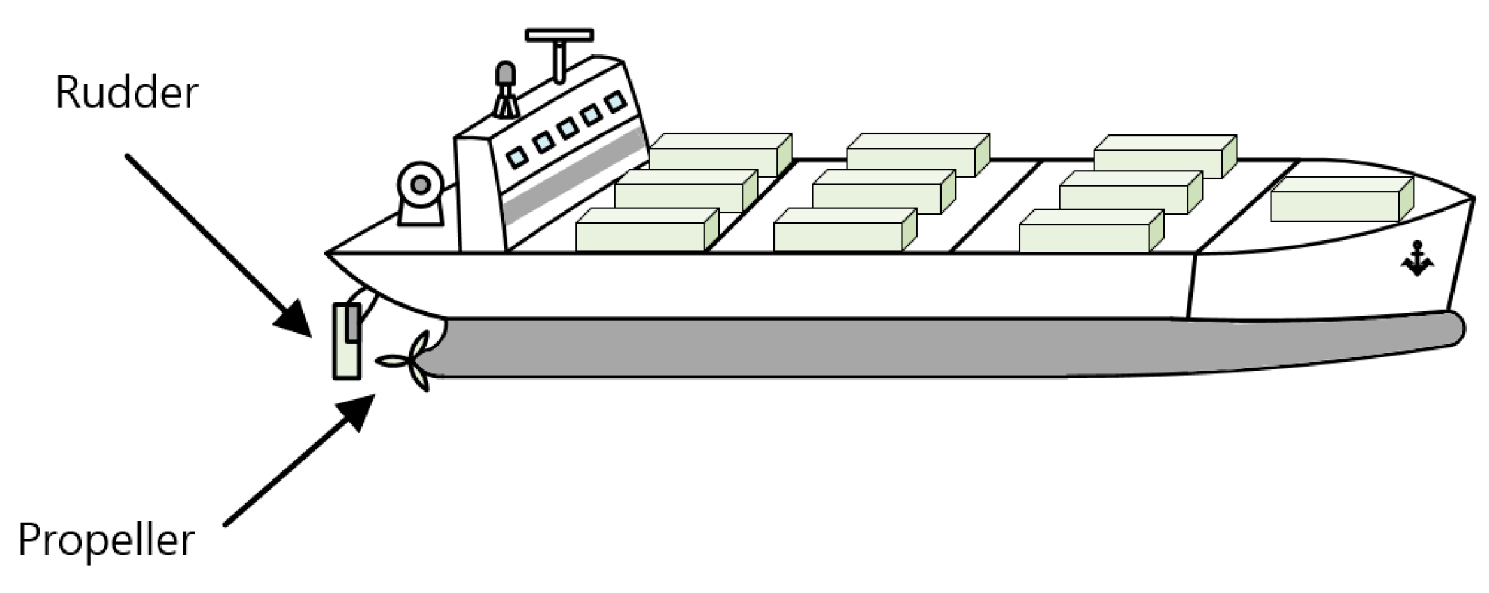
Figure 2 shows the vessel used in this study. The vessel consists of one propeller used to generate thrust and one rudder used to control the heading angle. The specifications of the vessel are shown in

Table 2. Specifications of the vessel.

Parameter	Length/Volume	Parameter	Length/Volume
$L$	$171.8 \mathrm{m}$	$L_{pp}$	$160.93 \mathrm{m}$
$T$	$8.23 \mathrm{m}$	$B$	$23.17 \mathrm{m}$
$\nabla$	$18541{ \mathrm{m}}^3$

where $L, L_{pp}, T, B$, and $\nabla$ are the length of the vessel, length between perpendiculars, draft, maximum beam, and maximum displacement, respectively.

.

4. Optimal Route Generation

Generally, when officers conduct route planning, they intend to identify the optimal route that minimizes fuel consumption or navigation time. Conventionally, the optimal route has been determined based on officers’ professional knowledge.

However, the concept of the maritime autonomous surface ship has emerged with the Fourth Industrial Revolution and active research in artificial intelligence. Such vessels must autonomously plan their route by considering various surrounding conditions, rather than relying on officers’ professional knowledge. To achieve this purpose, an optimal route was generated based on reinforcement learning in this study.

4.1. Reinforcement-Learning Algorithm

4.1.1. Definition of Reinforcement Learning

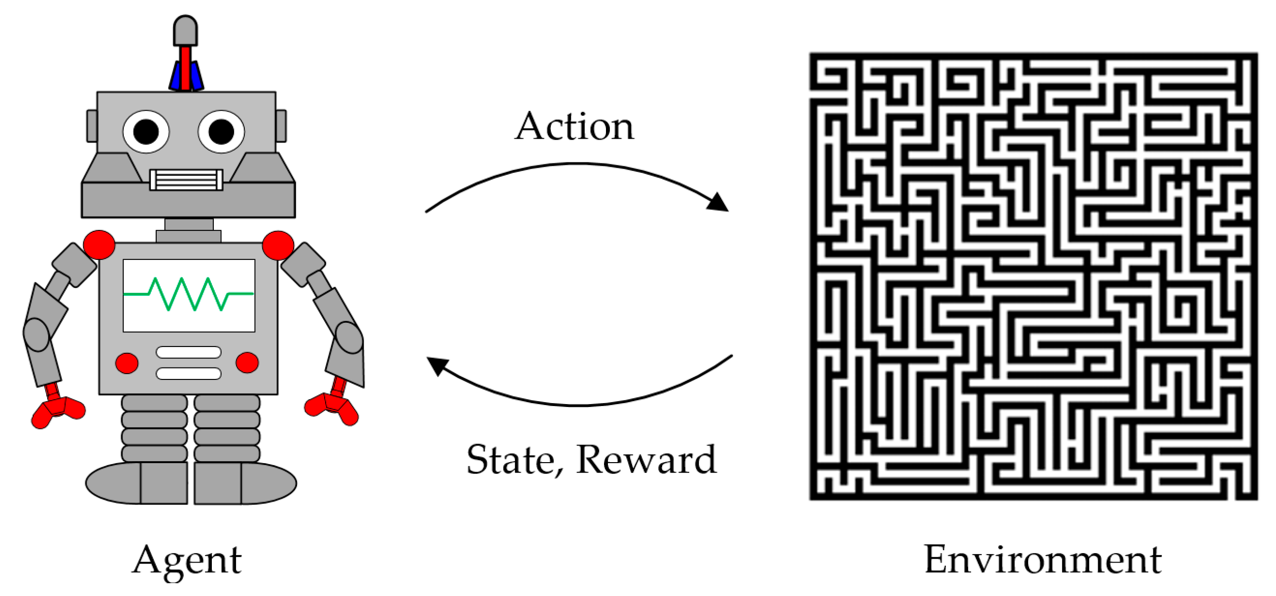
Figure 3 depicts the concept of reinforcement learning, in which an algorithm attempts to learn how to achieve a goal through the interaction between an agent and the environment. Reinforcement learning progresses through the following sequence [51,52]:

(1)

The agent observes the current state $\left(S_t\right)$.

(2)

The agent uses $S_t$ to perform a suitable action $\left(A_t\right)$ and provides it to the environment.

(3)

The environment communicates the next state $\left(S_{t+1}\right)$ and reward for the action to the agent.

(4)

The agent performs the next action according to the reward received from the environment.

(5)

By repeating the above processes, the agent continuously implements actions to obtain the maximum reward.

4.1.2. Selection of Reinforcement-Learning Algorithm

The agent has multiple components, which include the policy, the value function, and the model. The policy is the factor that determines how the agent behaves in a particular state, the value function is the factor that evaluates the effectiveness of each state/action, and the model is the environment from the agent’s perspective.

The types of reinforcement learning performed according to learning methods that involve a policy, value function, and model are expressed in the following figure.

As shown in Figure 4, reinforcement-learning algorithms can be divided into model-based and model-free types according to the learning method. Model-free reinforcement learning can be further divided into value-based and policy-based types.

Dynamic programming (DP) is a representative example of a model-based reinforcement-learning algorithm. DP can be applied when the designer knows about the environment, and it can easily solve problems very efficiently. However, DP has significant limitations, including computational complexity and the requirement for complete information regarding the environment. DP solves problems on the assumption that the designer knows the exact probability of reward and state transformation; therefore, it is difficult to use DP if the designer does not have precise information regarding the environment.

REINFORCE is a representative example of a policy-based reinforcement-learning algorithm. Policy-based reinforcement algorithms are mainly used when the action space is continuous. However, this algorithm is not suitable for learning data that are outdated, because the best behavior is policy dependent. Additionally, because data can only be learned for each episode, a long learning interval is required if the episode length is long.

SARSA, Q-learning, DQN, and Monte Carlo are representative examples of value-based reinforcement-learning algorithms. Unlike policy-based algorithms, these algorithms are widely used when the action space is discrete. Because the route is generated based on pixels, the action space is discrete (Figure 5).

Figure 5 shows the action space an agent can take to generate a route on a pixel. The agent can take actions in eight directions; thus, their actions are discrete.

SARSA is a representative on-policy control algorithm that updates the value function after taking the next action in the next state (i.e., the agent learns as it behaves). A limitation of the SARSA algorithm is that if learning initially proceeds in the wrong direction, it will continue in the wrong direction.

In contrast, Q-learning is an off-policy that updates the value function without taking the next action in the next state. Therefore, even if learning initially proceeds in the wrong direction, learning can proceed correctly because the action in the next state is not used to update the value function.

DQN, an algorithm that attaches a neural network to the Q-learning algorithm, is widely used when the number of states is very large (dynamic environment). In this study, the Q-learning algorithm was applied because it can generate an optimal route between the port of departure and entry in a state where the environment does not move.

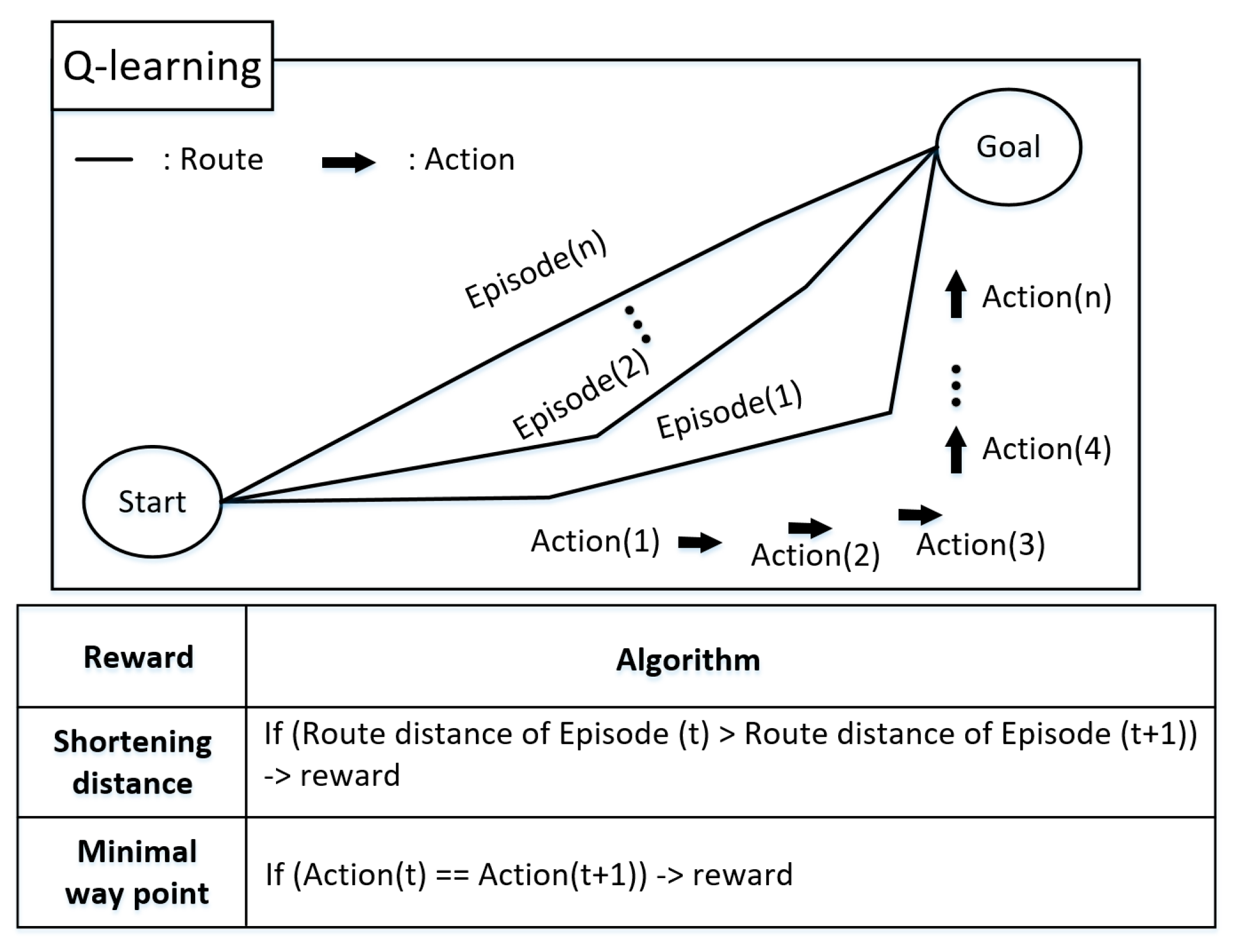
Figure 6 shows the concept of the Q-learning algorithm. The Q-learning algorithm uses $\left(S_t,A_t,R_{t+1},S_{t+1}\right)$ as a sample; it uses the largest Q-function in the next state to update the current Q-function. Accordingly, the Q-learning algorithm uses the maximum Q-function of the next state when selecting the Q-function of the current state, regardless of which action is taken in the next state.

The concept of the Q-learning algorithm is as follows [53,54]:

In this manner, the process of updating the Q-function is expressed as follows:

$$Q\left(S_t,A_t\right)\leftarrow Q\left(S_t,A_t\right)+\alpha \left(R+\gamma maxQ\left(S_{t+1},a^{\prime }\right)-Q\left(S_t,A_t\right)\right)$$

(16)

where $\alpha$ and $\gamma$ are the learning rate and discount factor, respectively. $\alpha$ is a parameter indicating how detailed the model will learn, and $\gamma$ is the rate at which the reward received in the future is reduced when considering it at present.

4.2. Considerations for Optimal Route Generation

4.2.1. Definition of the Optimal Route

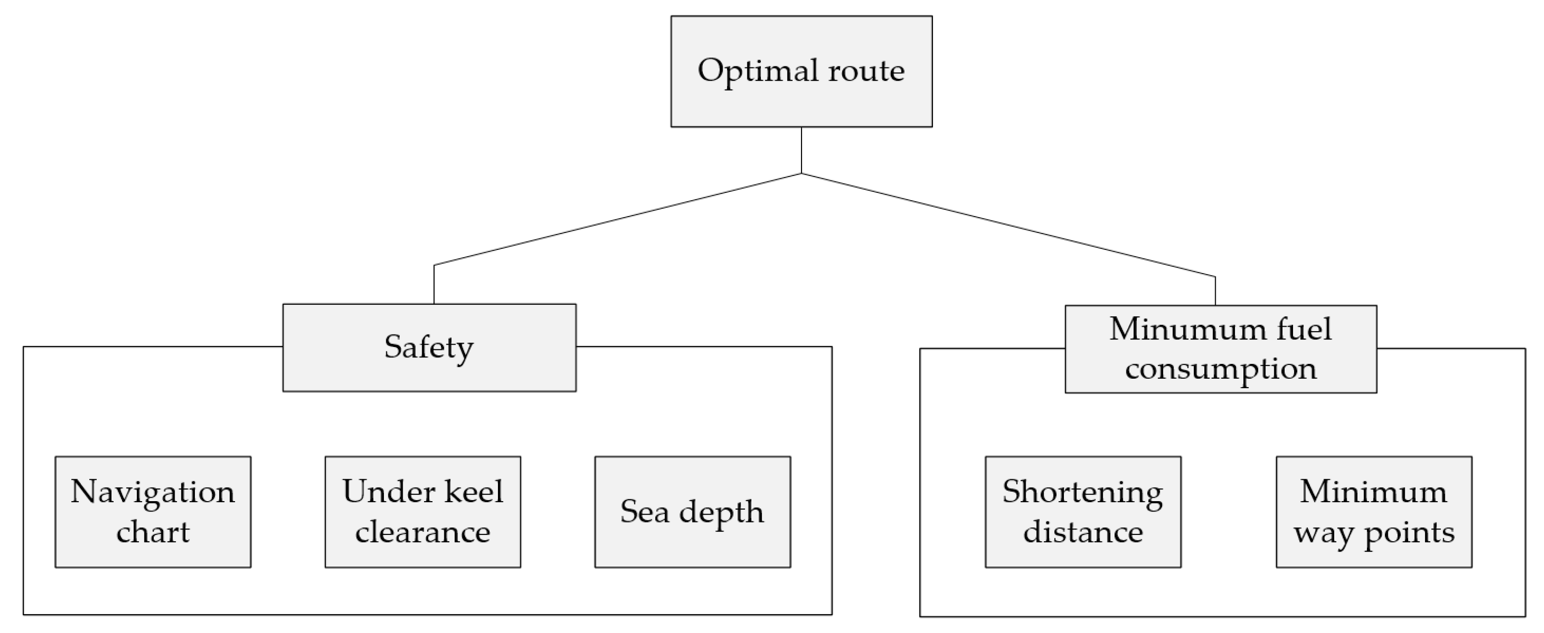
The optimal route defined in this study is shown in Figure 7.

Figure 7 shows the concept of the optimal route defined in this study. We attempted to plan an optimal route that ensured vessel safety and minimum fuel consumption by the vessel.

First, to satisfy the requirement of vessel safety, planning reflected the navigation chart information, under-keel clearance ($UKC$), and sea depth. In the offshore environment, many vessels may be passing through the area, and traffic may be congested; thus, navigation charts were used to ensure that mutual navigation rules were observed. Additionally, to prevent the vessel sinking and being stranded, $UKC$ was selected according to the vessel’s specifications; vessels were also allowed to operate only at a specific sea depth.

Second, to satisfy the requirement for minimum fuel consumption, planning reflected the shortening distance and minimum waypoints. To reduce fuel consumption, it is essential to shorten the distance of the route. Additionally, because frequent course alterations increase vessel energy consumption, the number of waypoints was minimized.

4.2.2. Data Used to Satisfy Safety Requirements

The navigation chart was provided by Korea Ocean Development Co., Ltd. (KORDO); sea depth data were provided by General Bathymetric Chart of the Ocean (GEBCO). To ensure vessel safety, the $UKC$ to guarantee the minimum sea depth can be obtained using the following equation [55]:

$$H-T_{max}>UKC, UKC=\beta T_{max}$$

(17)

where $H$, $T_{max}$, and $\beta$ are the sea depth, maximum draft of the vessel, and coefficient of $UKC$, respectively. $UKC$ is determined according to the influence of waves; it is generally regarded as 0.1 to 0.15 for seas with slight wave influence, and 0.3 for seas with large wave influence.

4.2.3. Algorithm Used to Satisfy Minimum Fuel Consumption

We intended to shorten the distance of the route to save fuel and sailing time, while minimizing the number of waypoints that would reduce vessel energy efficiency. To satisfy these conditions, the following algorithm was utilized to train the Q-learning model.

Figure 8 shows the algorithm to minimize vessel fuel consumption. To shorten the distance of the route, if the distance of the $t+1$th episode is shorter than the distance of the $t$th episode, a reward is given. To avoid creating unnecessary waypoints, if the $t$th action and $t+1$th action are identical, a reward is given.

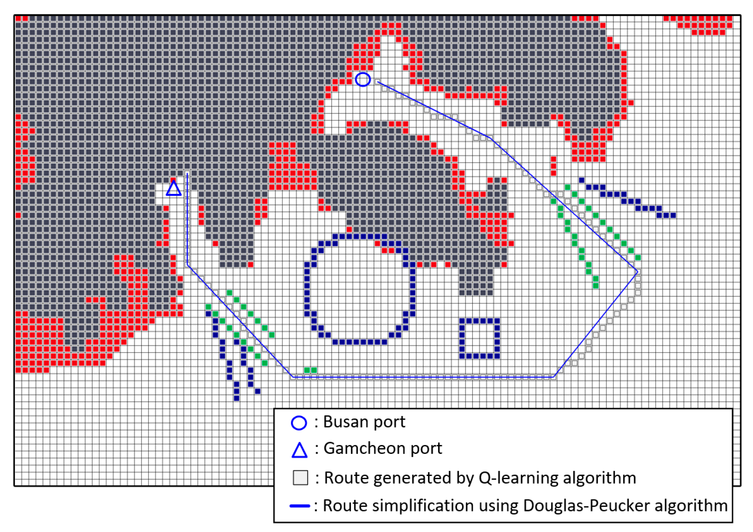
However, because the Q-learning algorithm searches for a route in units of pixels, it has a disadvantage in that the generated route inevitably does not lead to the minimum straight line. Such phenomena also cause the creation of unnecessary waypoints.

Therefore, the route must be simplified, and unnecessary waypoints must be removed by utilizing an algorithm that connects the route with a straight line. In this study, the Douglas–Peucker algorithm was applied to connect the route in a straight line.

4.3. Generation of the Optimal Route Using a Q-Learning Algorithm

In this study, the route was intended to be generated under conditions whereby a vessel departs from Busan port and arrives at Gamcheon port. The latitudes and longitudes of the target areas are $\left({34}^{°}{59}^{\prime }{37}^{″} ~ {35}^{°}{07}^{\prime }{52}^{″}\right)$ and $\left({128}^{°}{57}^{\prime }{08}^{″} ~ {129}^{°}{09}^{\prime }{37}^{″}\right)$.

4.3.1. Environment Settings for Training the Q-Learning Algorithm

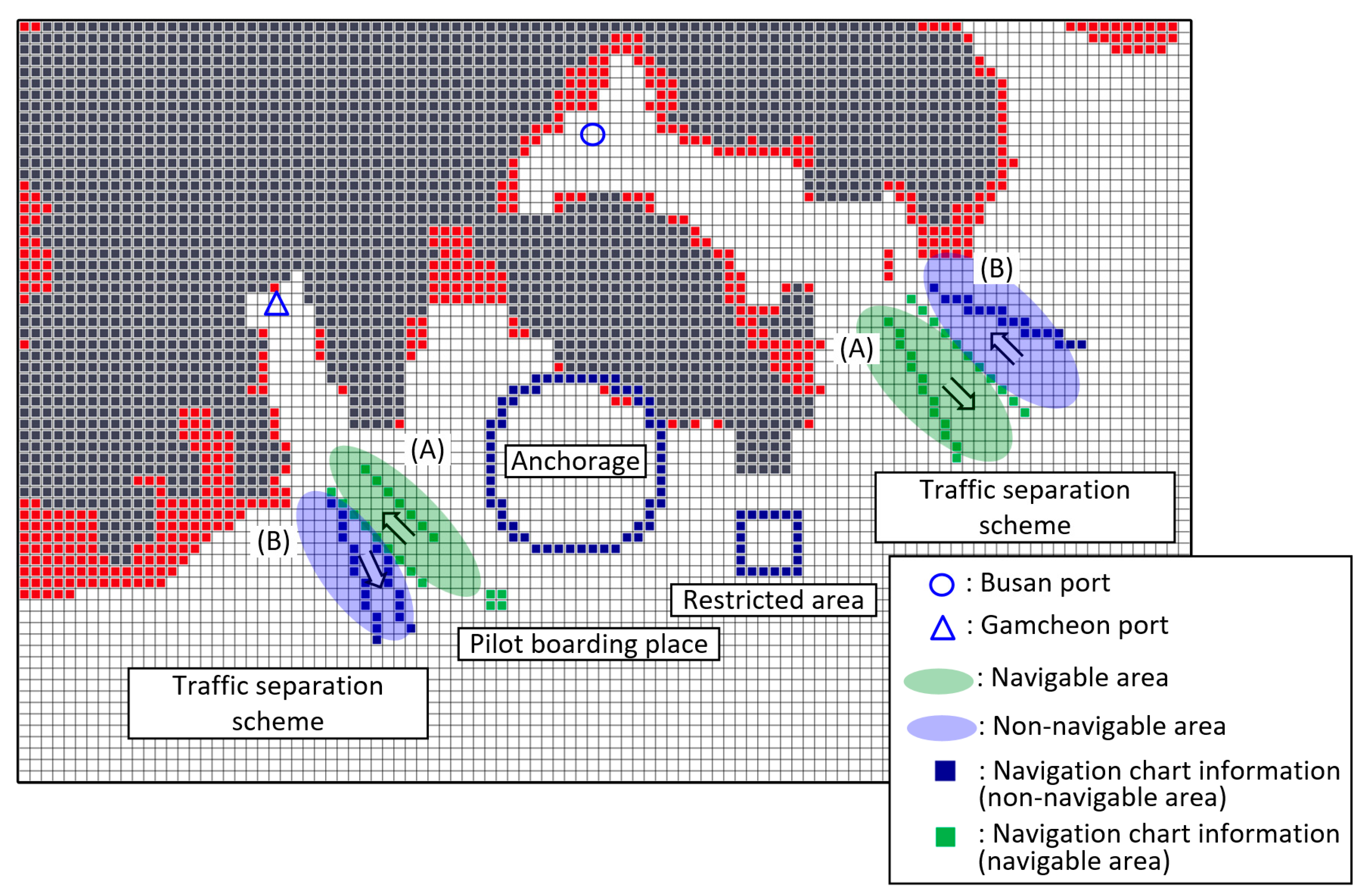
To generate the optimal route using the Q-learning algorithm, a training environment must be constructed by integrating the navigation chart information, $UKC$, and sea depth data.

The target area used in this study is an area that is significantly affected by waves; the coefficient of the $UKC$ was selected as $0.3$, and $UKC$ was calculated to be approximately $10.7 \mathrm{m}$ using Equation (17). Therefore, a $UKC$ of $11 \mathrm{m}$ was selected; areas with sea depth ≤$11 \mathrm{m}$ were regarded as restricted areas, where the vessel could not pass while satisfying the safety requirements.

The navigation chart information used is shown in

Table 3. Navigation chart information.

	Information
1	Restricted area
2	Pilot boarding place
3	Anchorage
4	Traffic separation scheme (Busan port)
5	Traffic separation scheme (Gamcheon port)

.

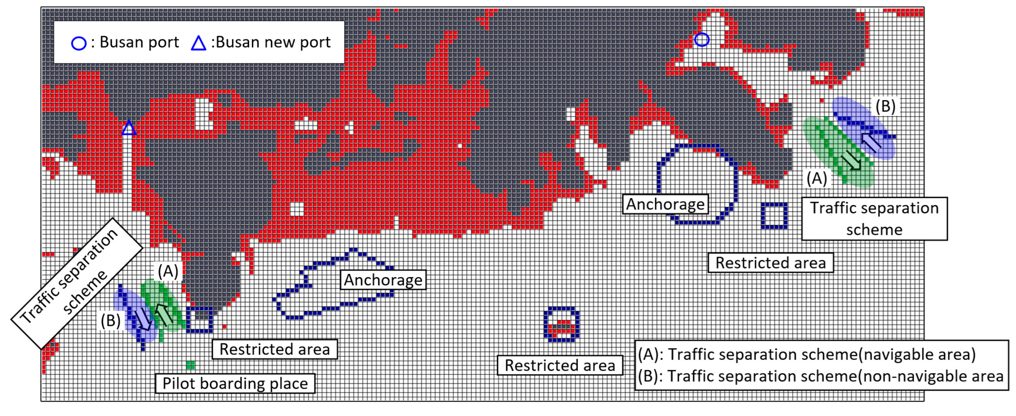
Table 3 shows the navigation chart information used in this study. First, a restricted area was applied around the island to prevent collisions and stranding. Second, when a vessel enters a port, it should be assisted by a pilot with detailed knowledge of the area; thus, a pilot boarding place was selected. Third, because vessels frequently wait at anchor to receive a signal to enter a port, a route could not be generated in the anchorage area. Finally, a traffic separation scheme was utilized to prevent accidents while entering and leaving the port. A traffic separation scheme is a system that separates the passage of large numbers of vessels; it constitutes an area designed in consideration of the traffic volume of passing vessels.

The integrated environment for generating an optimal route considering navigation chart information, $UKC$, and sea depth is shown in Figure 9.

Figure 9 shows the environment built to generate an optimal route. The blue circle is Busan port, the vessel’s departure point, and the blue triangle is Gamcheon port, the vessel’s destination point. Black squares represent land. Considering the $UKC$, areas where the sea depth is <$11 \mathrm{m}$ are shown as red squares, whereas areas with sea depth >$11 \mathrm{m}$ are shown as white squares. Additionally, navigation chart information is indicated by blue and green squares. For vessel safety, blue squares are areas (anchorage, restricted area, and traffic separation scheme (B)) through which the route may not pass; green squares are areas (pilot boarding place and traffic separation scheme (A)) through which the route must pass. Because this study involved departing from Busan port and arriving at Gamcheon port, the vessel must pass through area (A) and not pass through area (B) in the traffic separation scheme zone.

4.3.2. Simulation Condition

The conditions of parameter values and rewards of the Q-learning algorithm used for simulation are shown in

Table 4. Conditions of Parameter Values and Rewards.

Parameter Values
$ϵ$	0.2
$\alpha$	0.01
$\gamma$	0.9
Rewards
Land	End learning
Sea depth < $11 \mathrm{m}$	End learning
Traffic separation scheme (A), pilot boarding place	20
Traffic separation scheme (B), anchorage, restricted area	−20
Arrival at the port of entry	10
Shortening distance algorithm	100
Minimum waypoint algorithm	20

.

Table 4 shows the conditions of the parameter values and rewards of the Q-learning algorithm, where $ϵ$ is an $ϵ$-greedy policy, and to provide the agent with a sufficient learning experience, it is not to explore to the place where the value of Q-function is the largest with a probability of $ϵ$. $ϵ$ was selected as 0.2, and $\alpha$ and $\gamma$ were selected as 0.01 and 0.9, respectively. In addition, the reward was set as follows. First of all, in order to shorten the training time, learning was terminated immediately when the vessel entered the area (land and sea depth <$11 \mathrm{m}$) into which it should not go. If the agent was located in areas corresponding to traffic separation scheme (A) and the pilot boarding place, through which the route must pass, 20 was given as a reward, and if the agent was located in areas corresponding to traffic separation scheme (B), anchorage, and restricted, through which the route must not pass, −20 was given as a penalty. When the agent arrived at the port of entry in the process of searching, 10 was given as a reward, and when the shortening distance and minimum waypoint algorithms were satisfied, 100 and 20 were given as rewards.

4.3.3. Simulation Results

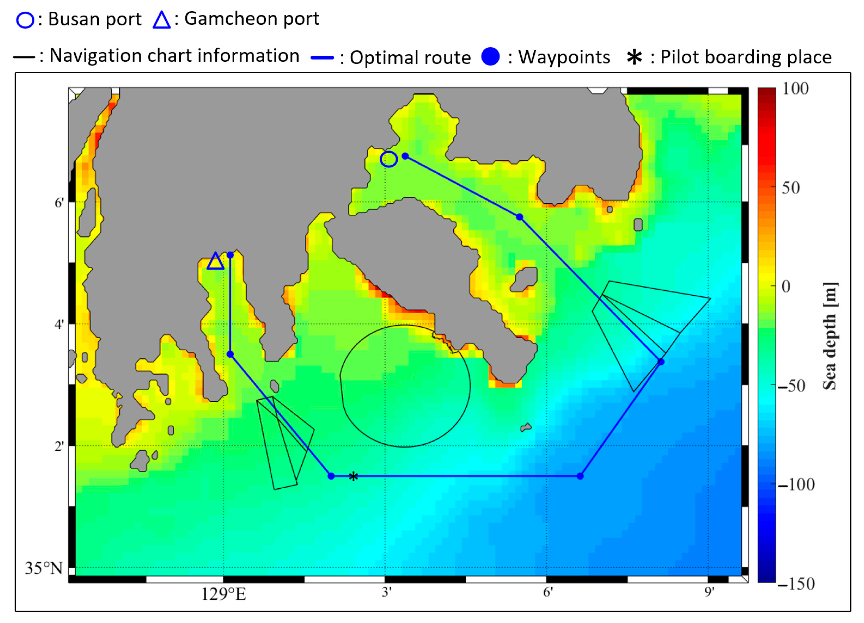
Figure 10 shows the optimal route generated by utilizing the Q-learning algorithm and the Douglas–Peucker algorithm. Because the Q-learning algorithm tends to maximize the reward, routes are consistently generated through the areas where rewards are given. Additionally, no routes are generated where penalties are applied. Based on the simulation with Q-learning, because the route is generated in pixel units, the route distance increases, and many unnecessary waypoints are generated. To compensate for this issue, the Douglas–Peucker algorithm was utilized to simplify the route generated by the Q-learning algorithm. As a result of simplifying the route, it was confirmed that the distance of the route was reduced, and the number of waypoints was significantly reduced to 5. However, for officers to use the optimal route, it must be displayed on an actual map (Figure 11).

4.4. Comparison with $A^{*}$ Algorithm

In order to demonstrate the excellence of the algorithm generated by Q-learning proposed in this study, we compared and analyzed its performance with the $A^{*}$ algorithm, which is widely used in path generation. The $A^{*}$ algorithm was simulated in the same environment that used for Q-learning, as shown in Figure 9.

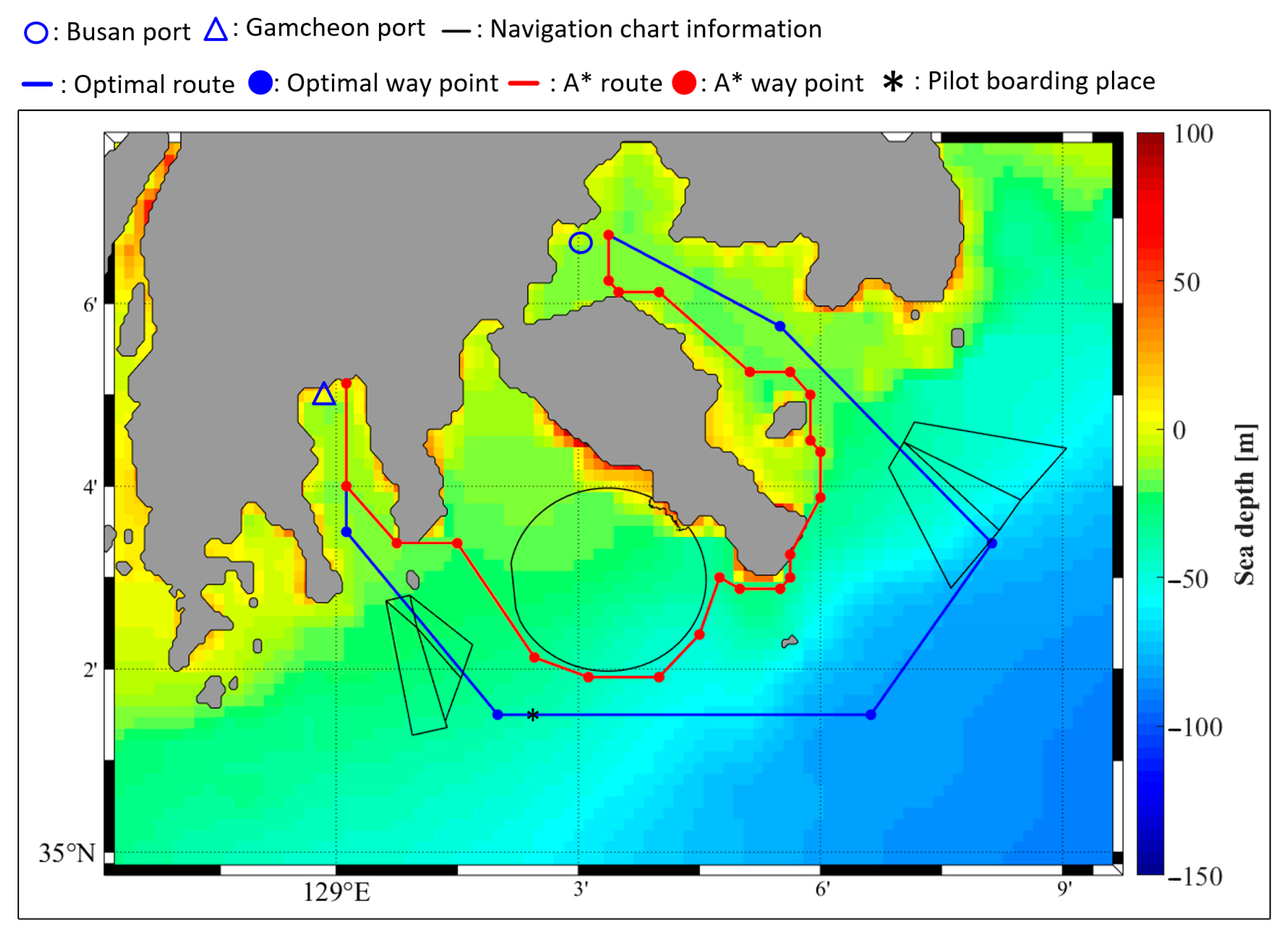
Figure 12 presents the simulation results, showing the optimal route based on the Q-learning and $A^{*}$ algorithms. $A^{*}$ is an algorithm that simply finds the shortest distance by judging areas that cannot be reached and areas that can be reached. Therefore, as shown in Figure 12, it can be confirmed that no route is generated in the areas (Land, anchorage, restricted area, Sea depth < $11 \mathrm{m}$, and Traffic separation scheme (B)) to be avoided, but it does not pass through areas (Traffic separation scheme (A) and Pilot boarding place) that need to be passed through. In addition, since a route is generated that is too close to the land, it is difficult to secure the stability of the vessel’s operation, and many unnecessary waypoints are generated, resulting in energy loss to the vessel.

The optimal route generated by the Q-learning algorithm has a disadvantage in that the distance of the route is longer than that of the $A^{*}$ algorithm. However, it can be confirmed that the number of unnecessary waypoints is significantly reduced. In addition, since the route is generated based on reward, it can be confirmed that the route is generated while satisfying the vessel’s operation regulations. In vessel operation, it is very important to pass the pilot boarding place and the Traffic separation scheme (A) area to ensure the safety of the vessel.

To verify the effectiveness of the reinforcement learning-based route generation methodology proposed in this study, an optimal route was generated targeting another area. Details on this are presented in Appendix A.

5. Route-Following Control

Section 5 addresses the control method for following the route. After the route has been determined, control technology to accurately maintain the route is required. PD controllers with simple structures and proven stability have been widely used to control vessel routes. However, the PD controller tends to deviate from the route because of overshoot when the course alteration angle is large and the speed is slow. Additionally, the rudder angle substantially changes, reducing vessel energy efficiency. To compensate for these problems, a velocity-type fuzzy PID controller was designed and used as a route-following controller in this study.

5.1. Design of the Velocity-Type Fuzzy PID Controller

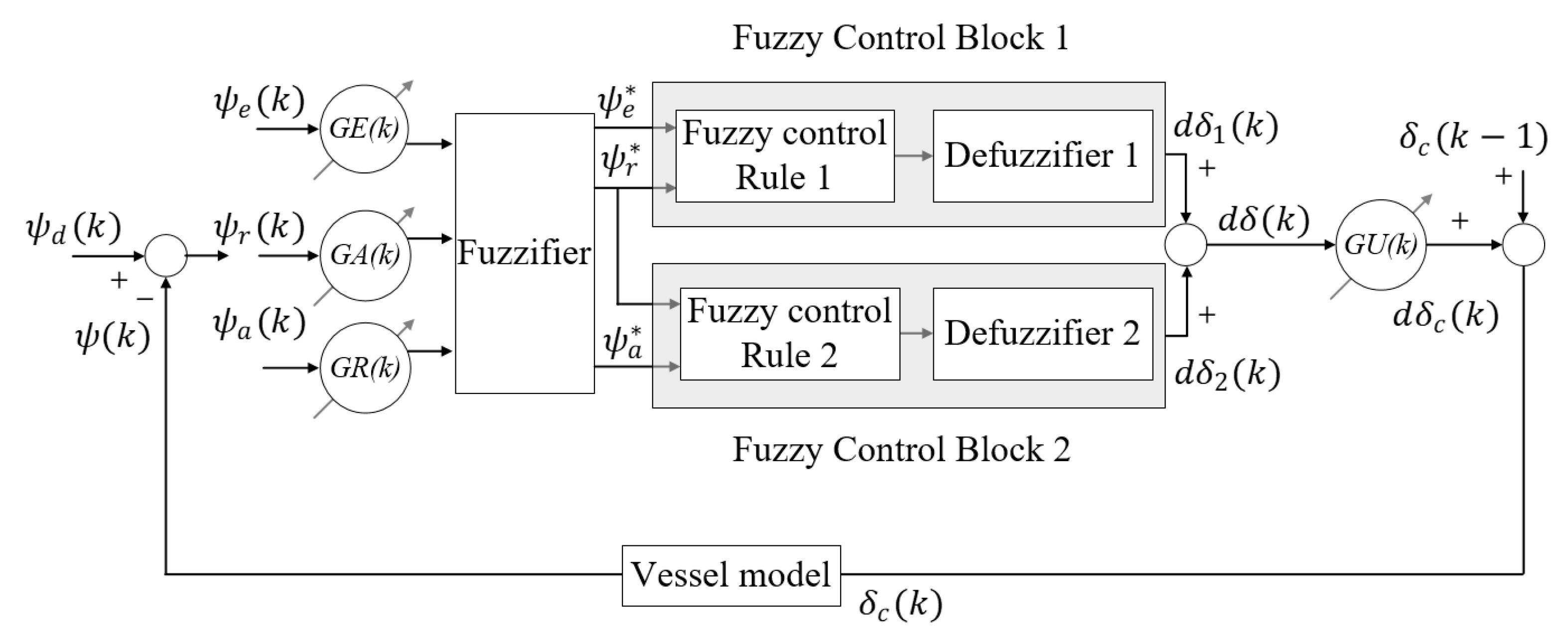
Figure 13 shows the structure of the velocity-type fuzzy PID controller. The velocity-type fuzzy PID controller uses the heading angle error, along with its velocity and acceleration, as input; the control increment of the rudder angle is generated as output. The variables used from input to output are expressed as follows [56]:

$$\begin{gathered} {\psi }_e\left(k\right)={\psi }_d\left(k\right)-\psi \left(k\right) \\ {\psi }_r\left(k\right)=\left[ {\psi }_e\left(k\right)-{\psi }_e\left(k-1\right)\right]/T \\ {\psi }_a\left(k\right)=\left[ {\psi }_r\left(k\right)-{\psi }_r\left(k-1\right)\right]/T \\ {\psi }_e^{*}=GE\left(k\right)\times {\psi }_e\left(k\right), {\psi }_r^{*}=GR\left(k\right)\times {\psi }_r\left(k\right), {\psi }_a^{*}=GA\left(k\right)\times {\psi }_a\left(k\right) \\ d\delta \left(k\right)=d{\delta }_1\left(k\right)+d{\delta }_2\left(k\right) \\ d{\delta }_c\left(k\right)=GU\left(k\right)\times d\delta \left(k\right), {\delta }_c\left(k\right)=d{\delta }_c\left(k\right)+{\delta }_c\left(k-1\right) \end{gathered}$$

(18)

where ${\psi }_d\left(k\right)$ and $\psi \left(k\right)$ are the reference heading angle and current heading angle of the vessel, respectively. ${\psi }_e\left(k\right)$, ${\psi }_r\left(k\right)$, and ${\psi }_a\left(k\right)$ are the error of heading angle, velocity of ${\psi }_e\left(k\right)$, and acceleration of ${\psi }_e\left(k\right)$ at sampling time $k$, respectively. $GE\left(k\right)$, $GR\left(k\right)$, and $GA\left(k\right)$ are the fuzzification scale parameters for ${\psi }_e^{*}$, ${\psi }_r^{*}$, and ${\psi }_a^{*}$, respectively. $GU\left(k\right)$ is the fuzzification scale parameter for $d{\delta }_c\left(k\right)$. The outputs of fuzzy control blocks 1 and 2, $d{\delta }_1\left(k\right)$ and $d{\delta }_2\left(k\right)$, are added to produce $d\delta \left(k\right)$. Furthermore, the control input ${\delta }_c\left(k\right)$ is created by adding the control increment $d{\delta }_c\left(k\right)$ and rudder angle at sampling time $k-1$.

5.1.1. Fuzzification Algorithm

Figure 14 shows the fuzzification algorithm for the inputs and outputs of the velocity-type fuzzy PID controller. The fuzzy set ${\psi }_e^{*}$ has two members: error positive ($EP$) and error negative ($EN$); the fuzzy set ${\psi }_r^{*}$ has two members: rate positive ($RP$) and ($RN$); and the fuzzy set ${\psi }_a^{*}$ has two members: error positive ($AP$) and error negative (A$N$) (Figure 14a). The fuzzy set $d{\delta }_1\left(k\right)$ has three members: output positive ($OP$), output zero ($\mathit{OZ}$), and output negative ($OP$) (Figure 14b); and the fuzzy set $d{\delta }_2\left(k\right)$ has two members: output positive middle ($OPM$) and output negative middle ($ONM$) (Figure 14c).

The fuzzification algorithms for $d{\delta }_1\left(k\right)$ and $d{\delta }_2\left(k\right)$ are different because fuzzy control block 2 compensates for the behavior of fuzzy control block 1. Fuzzy control block 2 has the ability to improve the transient response of the system.

5.1.2. Fuzzy Control Rule

Fuzzy control rules are created based on expert experience and control engineering knowledge [57,58,59,60]. The fuzzy control rules for fuzzy control blocks 1 and 2 used in this study are shown in

Table 5. Fuzzy control rules for fuzzy control blocks 1 and 2.

Fuzzy Control Block 1

${\left(R1\right)}_1: IF {\psi }_e^{*}=EP and {\psi }_r^{*}=RP THEN d{\delta }_1\left(k\right)=OP$

${\left(R2\right)}_1: IF {\psi }_e^{*}=EP and {\psi }_r^{*}=RN THEN d{\delta }_1\left(k\right)=OZ$

${\left(R3\right)}_1: IF {\psi }_e^{*}=EN and {\psi }_r^{*}=RP THEN d{\delta }_1\left(k\right)=OZ$

${\left(R4\right)}_1: IF {\psi }_e^{*}=EN and {\psi }_r^{*}=RN THEN d{\delta }_1\left(k\right)=ON$

Fuzzy Control Block 2

${\left(R1\right)}_2: IF {\psi }_r^{*}=RP and {\psi }_a^{*}=AP THEN d{\delta }_2\left(k\right)=OPM$

${\left(R2\right)}_2: IF {\psi }_r^{*}=RP and {\psi }_a^{*}=AN THEN d{\delta }_2\left(k\right)=ONM$

${\left(R3\right)}_2: IF {\psi }_r^{*}=RN and {\psi }_a^{*}=AP THEN d{\delta }_2\left(k\right)=OPM$

${\left(R4\right)}_2: IF {\psi }_r^{*}=RN and {\psi }_a^{*}=AN THEN d{\delta }_2\left(k\right)=ONM$

.

In fuzzy control $\left({\left(R1\right)}_1 ~ {\left(R4\right)}_1\right)$, ${\left(R1\right)}_2 ~ {\left(R4\right)}_2)$, Zedeh’s AND logic is utilized to determine the first half of each rule, and Lukasiewicz OR logic is utilized to combine each rule.

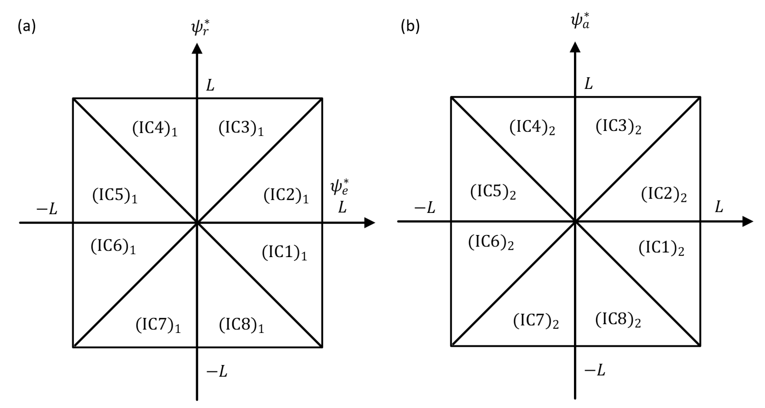
If the scale parameters are varied at each sampling time, as shown in Equation (19), such that inputs always exist within the range of the normalization parameter $L$ according to the size of the input, input combinations for fuzzy control blocks 1 and 2 can be generated as shown below.

$$GE\left(k\right)=\frac{L}{{\psi }_e\left(k\right)}, GR\left(k\right)=\frac{L}{{\psi }_r\left(k\right)}, GA\left(k\right)=\frac{L}{{\psi }_a\left(k\right)}$$

(19)

5.1.3. Defuzzification Algorithm

The center of area method [61,62,63] is utilized as the defuzzification approached used in the velocity fuzzy PID controller, and the following defuzzification output is generated [64]:

$$d{\delta }_j\left(k\right)=\frac{{{\displaystyle \sum }}_{i=1}^n{\mu }_{d{\delta }_j\left(k\right)}\left(w_i\right)\times \left(w_i\right)}{{{\displaystyle \sum }}_{i=1}^n{\mu }_{d{\delta }_j\left(k\right)}\left(w_i\right)}$$

(20)

where $j$ represents the outputs of fuzzy control blocks 1 and 2, with values of 1 and 2; $n$ is the number of rules corresponding to each fuzzy control block, with a value of 4; and $w_i$ and ${\mu }_{d{\delta }_j\left(k\right)}\left(w_i\right)$ are the member values and membership of a member, respectively.

For fuzzy control blocks 1 and 2, output fuzzy sets are defuzzified within $L$ interval to generate $d{\delta }_1\left(k\right)$ and $d{\delta }_2\left(k\right)$. Then, the final control increment $d{\delta }_c\left(k\right)$ can be generated through the addition of $d{\delta }_1\left(k\right)$ and $d{\delta }_2\left(k\right)$ and multiplication by the output scale parameter $GU\left(k\right)$.

If the control increment $d{\delta }_c\left(k\right)$ is arranged and simplified according to the input combinations condition as shown in Figure 15, a very simple PID-type control increment is created, as shown in the equation below:

$$d{\delta }_c\left(k\right)=K_i\left(k\right){\psi }_e\left(k\right)+K_p\left(k\right){\psi }_r\left(k\right)+K_d\left(k\right){\psi }_a\left(k\right)$$

(21)

where $K_i\left(k\right)$, $K_p\left(k\right)$, and $K_d\left(k\right)$ are defined as integral gain, proportional gain, and derivative gain, respectively. The gain values are obtained according to the following equations:

$$\begin{gathered} K_i\left(k\right)=0.5\times GU\left(k\right)\times GE\left(k\right) \\ {K}_p\left(k\right)=0.5\times GU\left(k\right)\times GR\left(k\right) \\ {K}_d\left(k\right)=0.25\times GU\left(k\right)\times GA\left(k\right) \end{gathered}$$

(22)

5.2. Performance Verification of Velocity-Type Fuzzy PID Controller

A simulation was conducted to find the optimal route from Busan port to Gamcheon port, as generated in Section 3, to verify the performance of the velocity-type fuzzy PID controller designed in this study; its performance was compared with the PD controller.

5.2.1. Simulation Condition

The PD controller used in this simulation is shown in Equation (23):

$$\delta \left(k\right)=-K_p\left({\psi }_d\left(k\right)-\psi \left(k\right)\right)+K_{d}r\left(k\right)$$

(23)

$K_p$ and $K_d$ were optimally selected as 1 and 70, respectively. The desired heading angle ${\psi }_d\left(k\right)$, defined as the angle between the vessel’s current position and the next position of the waypoint, was expressed as follows:

$${\psi }_d\left(k\right)=atan2\left(y_k-y\left(k\right), x_k-x\left(k\right)\right)$$

(24)

where $x_k$ and $y_k$ are the coordinates corresponding to the x- and y-axes of the next waypoint, respectively; $x\left(k\right)$ and $y\left(k\right)$ are coordinates corresponding to the x- and y-axes of the current vessel position.

The vessel’s forward velocity was set to $8 \mathrm{m}/\mathrm{s}$, and the maximum allowable angle of the rudder was limited to $\pm {20}^{°}$ to ensure vessel stability.

5.2.2. Simulation Results for the Route-Following Control

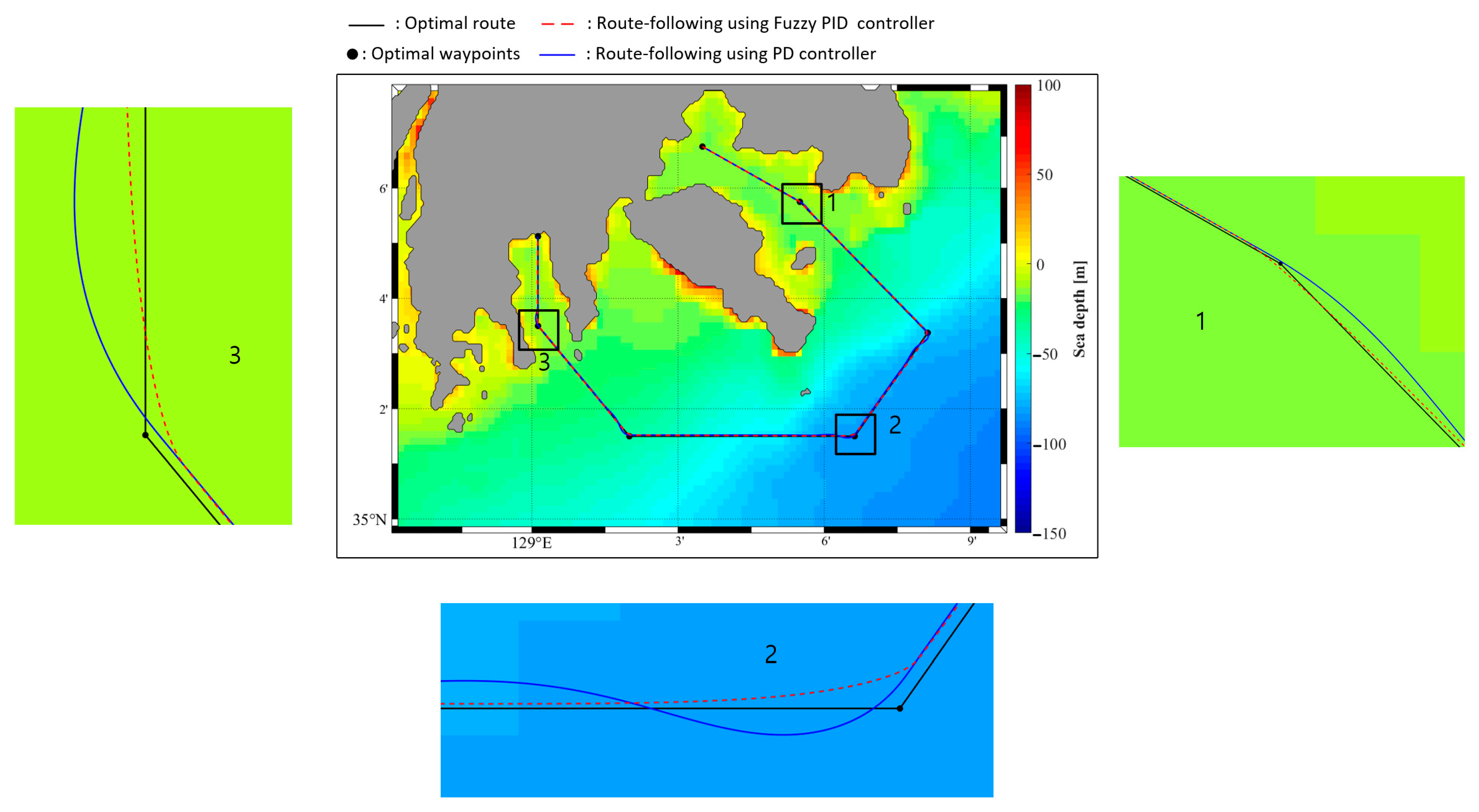
Figure 16 shows the simulation results of route-following using PD and velocity-type fuzzy PID controllers. Both controllers generally demonstrated good adherence to the optimal route.

However, if course alteration Section 1, Section 2 and Section 3 were enlarged, the limitations of the PD controller expressed as a blue solid line were confirmed. When the PD controller was used, a larger course alteration angle was associated with larger overshoot, resulting in route deviation. Additionally, the vessel required a long interval to become stabilized.

In contrast, when the velocity-type fuzzy PID controller was used, the route was followed reliably, with overshoot rarely occurring, regardless of the magnitude of the angle of the later course. Such results demonstrate that the vessel can accurately follow the designated route.

The performance of the PD controller deteriorated because the gains of the controller could not be changed after they had been established. However, unlike the PD controller, the velocity-type fuzzy PID controller optimally scheduled the gains in real time according to the fuzzy control rules; thus, the performance of route-following control was superior to performance with the PD controller.

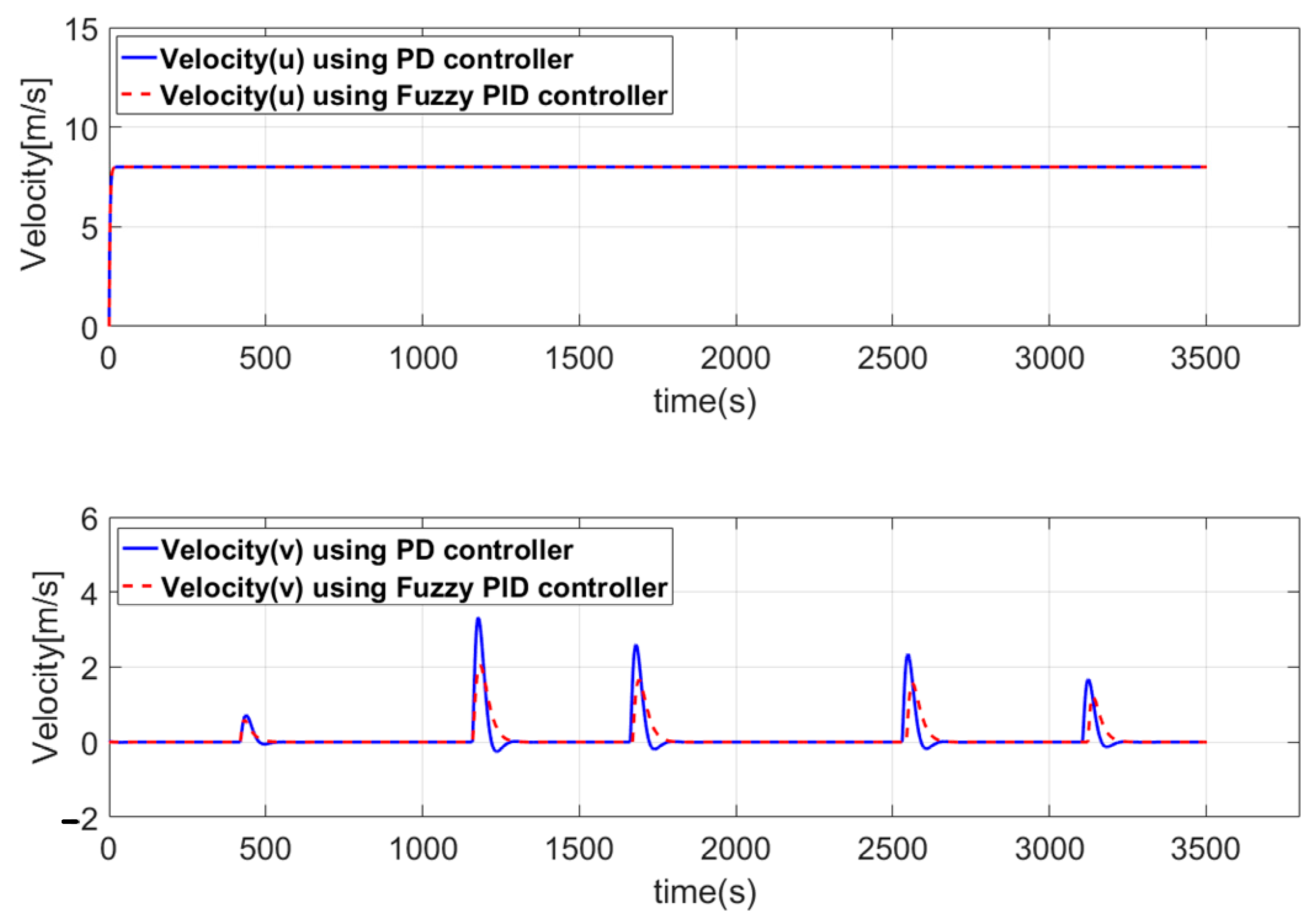
Figure 17 shows the simulation results for vessel velocities. Because the forward direction velocity was set to $8 \mathrm{m}/\mathrm{s}$, this value remained constant. There was no lateral velocity in the section except for the alter course; in the course alteration section, the PD controller had a higher absolute value of the later velocity than the velocity-type fuzzy PID controller. This difference was directly related to route deviation.

The route-following controller used the heading angle as an input and generated the rudder angle as an output to ensure that the vessel could follow the route. Therefore, Figure 18 and Figure 19 are important indicators regarding controller performance.

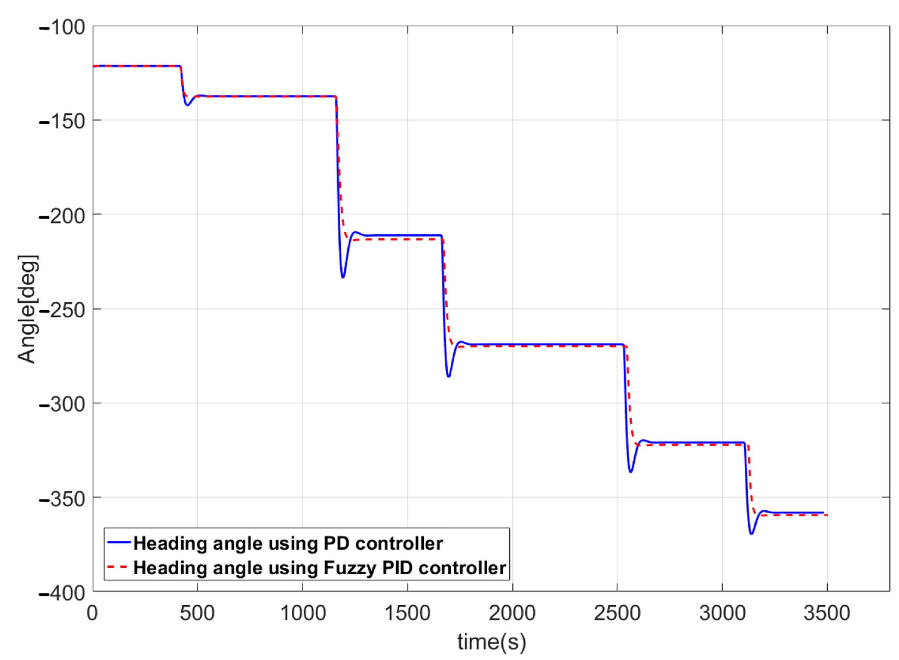
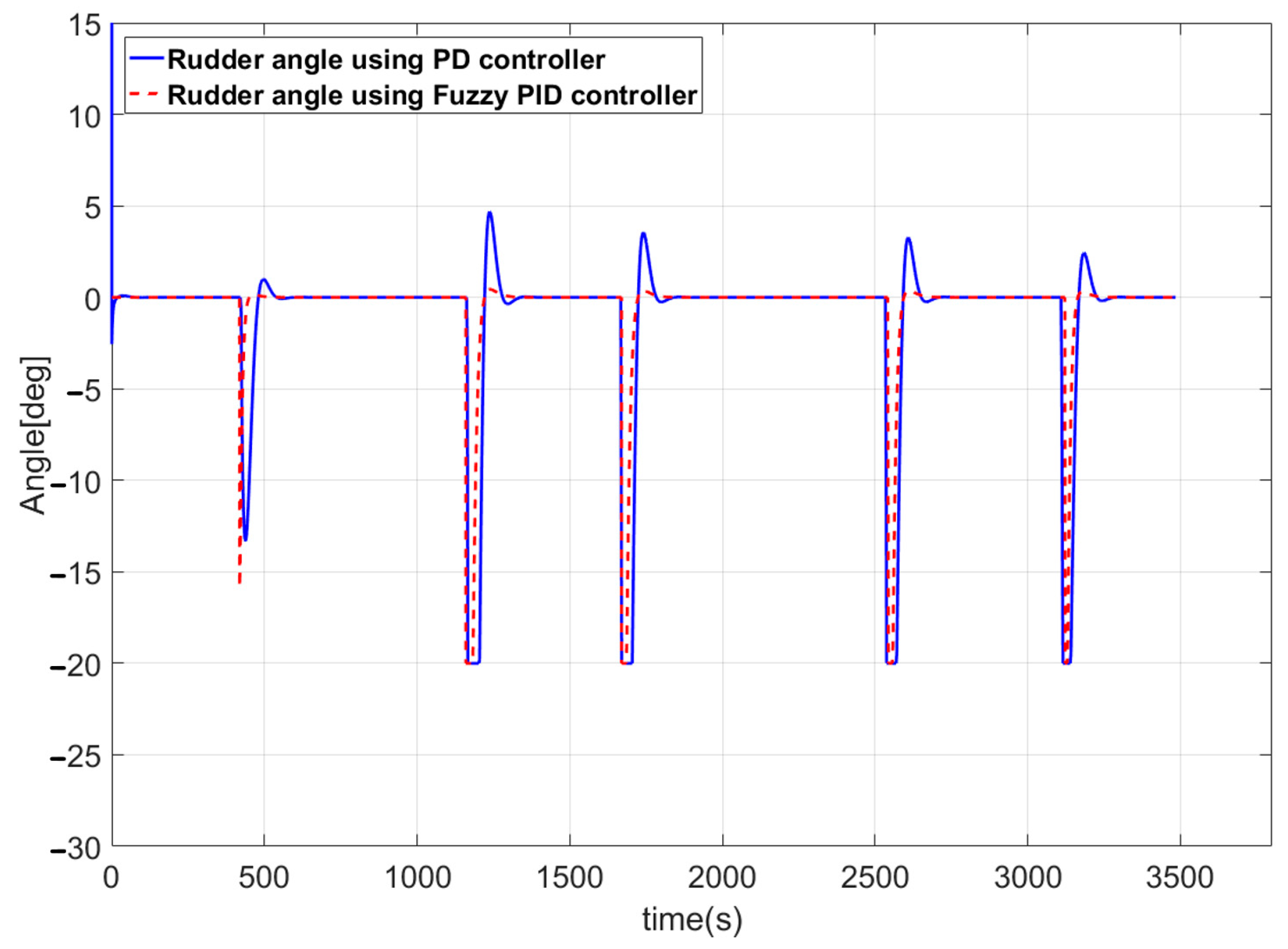
Figure 19 shows the simulation results of the rudder angle when the rudder was controlled using the PD and velocity-type fuzzy PID controllers. When the PD controller was used, the rudder angle changed in a rough manner, whereas the velocity-type fuzzy PID controller exhibited a smooth rudder angle change. In addition, it can be confirmed that the stabilization time of the vessel is short because the speed of the alter course is fast. This result arose because the velocity-type fuzzy PID controller was utilized as an input to the controller in incremental form. Therefore, upon application of the velocity-type fuzzy PID controller, a smooth vessel heading angle was generated without large overshoot (Figure 18).

A series of simulations confirmed the superiority of the velocity-type fuzzy PID controller; therefore, the velocity-type fuzzy PID controller was selected to follow the route in this study.

6. Estimation of Environmental Disturbances Using a Fuzzy Disturbance Estimator

In this study, a velocity-type fuzzy PID controller was applied to accurately follow the route. However, when a vessel actually sails, it is greatly affected by various environmental disturbances, including wind, waves, and ocean currents. The presence of such environmental disturbances will result in vessel deviation from the designated route, regardless of whether the velocity-type fuzzy PID controller is used. Additional energy is consumed to control the vessel, thus increasing the vessel’s energy use.

To solve these issues, Session 5 estimates the magnitude of environmental disturbances using the characteristics of the Kalman filter innovation. Additionally, if the estimated environmental disturbances are converted into the thrust and rudder angle to control the vessel and regarded as control input, the vessel will be able to accurately follow the designated route despite the environmental disturbances.

6.1. Method for Determining the Existence of Environmental Disturbances

Generally, if the Kalman filter succeeds in state estimation, the innovation process tends to chatter at $0$; if unknown disturbances are applied from the outside, state estimation fails, and the innovation process chatters with a constant DC value. Environmental disturbance has a meaning identical to unknown disturbance because its effects on the vessel are unknown.

In this context, the presence of environmental disturbance is determined. First, if the value of the innovation process at each sampling time is converted into an absolute value and averaged by summing over a specific number of sampling intervals, a value that does not considerably fluctuate can be obtained. The corresponding equation is shown below:

$$S=\left({\displaystyle \sum }_{j=0}^N\left|ie\left(k-i\right)\right|\right)/N$$

(25)

where $ie\left(k\right)$ is the innovation process at sampling time $k$ of the Kalman filter, defined as the difference between the output of the system and the value of the filter estimation; $N$ is the window defining the range of the number of the innovation process to be accumulated. If the window is excessively small, $ie\left(k\right)$ has a large influence on $S$; thus, it is sensitive to the latest information. Conversely, if the window is excessively large, $ie\left(k\right)$ does not have a large influence on $S$; thus, it is insensitive to the latest information.

Therefore, the size of the window is selected by the designer based on the required sensitivity. If the value of $S$, which does not considerably fluctuate, is obtained, the existence of environmental disturbance must be determined.

Figure 20 shows how to determine the existence of environmental disturbances. The threshold $\eta$ is a constant determined by the designer based on the value of $S$. If the condition $S>\eta$ is satisfied, environmental disturbance is applied to the vessel. Then, a fuzzy disturbance estimator is used to estimate the magnitude of the environmental disturbance $\widehat{est}\left(k\right)$. The fuzzy disturbance estimator for estimating the environmental disturbance is presented in Section 5.2 [65].

6.2. Design of the Fuzzy Disturbance Estimator

Figure 21 shows the structure of the fuzzy disturbance estimator. The overall structure is similar to the structure of the velocity-type fuzzy PID control shown in Figure 12, but there are differences in the variables used.

The velocity-type fuzzy PID controller uses the error components of the heading angle as input and generates control increment of the rudder angle as output. However, the fuzzy disturbance estimator uses the error components of the innovation process of the Kalman filter as input; it produces the estimated value of the environmental disturbance as output. The definitions of variables used in the fuzzy disturbance estimator are as follows:

$$\begin{gathered} ie\left(k\right)=z\left(k\right)-\widehat{z}\left(k\right), ie{\left(k\right)}^{*}=GIE\left(k\right)\times ie\left(k\right) \\ ir\left(k\right)=ie\left(k\right)/T, ir{\left(k\right)}^{*}=GIR\left(k\right)\times ir\left(k\right) \\ ia\left(k\right)=\left[ie\left(k\right)-ie\left(k-1\right)\right]/T, ia{\left(k\right)}^{*}=GIA\left(k\right)\times ia\left(k\right) \\ est\left(k\right)=est1\left(k\right)+est2\left(k\right), \widehat{est}\left(k\right)=est\left(k\right)\times GEST\left(k\right) \end{gathered}$$

(26)

where $ie\left(k\right)$, $ir\left(k\right)$, and $ia\left(k\right)$ are the innovation process, values obtained by dividing the $ie\left(k\right)$ by sampling time $T$, and rate of change according to sampling time of $ie\left(k\right)$, respectively. $GIE\left(k\right)$, $GIR\left(k\right)$, and $GIA\left(k\right)$ are the fuzzification scale parameters for $ie{\left(k\right)}^{*}$, $ir{\left(k\right)}^{*}$, and $ia{\left(k\right)}^{*}$, respectively. $GEST\left(k\right)$ is the fuzzification scale parameter for $\widehat{est}\left(k\right)$. The outputs of fuzzy estimation blocks 1 and 2, $est1\left(k\right)$ and $est2\left(k\right)$, are summed to produce $est\left(k\right)$. Additionally, the value of the estimated environmental disturbance $\widehat{est}\left(k\right)$ is created by multiplying $GEST\left(k\right).$

Because the fuzzification algorithm, fuzzy estimation rule, and defuzzification algorithm used in the fuzzy disturbance estimator are similar to those aspects of the velocity-type fuzzy PID controller, they are not discussed further in this paper.

The value of the environmental disturbance, estimated by the fuzzy disturbance estimator generated through the above process, is as follows:

$$\widehat{est}\left(k\right)=E_i\left(k\right)ie\left(k\right)+E_p\left(k\right)ir\left(k\right)+E_d\left(k\right)ia\left(k\right)$$

(27)

where $E_i\left(k\right)$, $E_p\left(k\right)$, and $E_d\left(k\right)$ are expressed as follows:

$$\begin{gathered} E_i\left(k\right)=0.5\times GEST\left(k\right)\times GIE\left(k\right) \\ {E}_p\left(k\right)=0.5\times GEST\left(k\right)\times GIR\left(k\right) \\ {E}_d\left(k\right)=0.25\times GEST\left(k\right)\times GIA\left(k\right) \end{gathered}$$

(28)

6.3. Route-Following Control System to Eliminate the Effects of Environmental Disturbance

Figure 22 shows a block diagram of the vessel’s route-following control system to eliminate the effects of environmental disturbance. If the environmental disturbance can be reliably estimated by the fuzzy disturbance estimator using the Kalman filter’s innovation process, it can be converted into thrust and rudder angle that control the vessel and feedback to the control input. Here, $T_{\widehat{est}}\left(k-1\right)$ and ${\delta }_{\widehat{est}}\left(k-1\right)$ are the values obtained by converting estimated environmental disturbance into thrust and rudder angle, respectively; ${\tau }_{dis}{}^{\prime }\left(k-1\right)$ is the environmental disturbance applied to the vessel; and $w\left(k-1\right)$ and $v\left(k\right)$ are the system noise and measurement noise, respectively.

6.4. Simulation of Route-Following Control

6.4.1. Simulation Conditions

Ocean currents, waves, and wind, which have major effects on vessels, were selected as the environmental disturbances in this study. Ocean currents were generated using a first-order Gauss–Markov process [66], and waves were generated by expressing the Perison–Moskowitz (PM) spectral density function in state space [67]. Finally, the method proposed by Isherwood was used to calculate the wind force and moment using wind force and moment coefficients, wind speed, and wind angle [68,69]. The simulation conditions for environmental disturbances are presented in

Table 6. Simulation conditions for environmental disturbances.

Conditions for Environmental Disturbances
$\mathrm{Wind} \mathrm{speed} \left(\mathrm{knot}\right)$	15
$\mathrm{Wind} \mathrm{direction} \left(\mathrm{deg}\right)$	−5
$\mathrm{Wave} \mathrm{amplitude} \left(\mathrm{m}\right)$	0.3
$\mathrm{Wave} \mathrm{period} \left(\mathrm{s}\right)$	10
$\mathrm{Ocean} \mathrm{current} \mathrm{average} \mathrm{speed} \left(\mathrm{m}/\mathrm{s}\right)$	1
$\mathrm{Ocean} \mathrm{current} \mathrm{direction} \left(\mathrm{deg}\right)$	−5

.

Table 6 presents the conditions for environmental disturbances selected in this study. The speed and direction of the wind were selected as 15$\mathrm{knot}$ and −5$\mathrm{deg}$, respectively, and the amplitude and period of the wave were selected as 0.3$\mathrm{m}$ and 10$\mathrm{s}$, respectively. In addition, average speed and direction of the ocean current were selected as 1$\mathrm{m}/\mathrm{s}$ and −5$\mathrm{deg}$, respectively.

The forward velocity and rudder limit angle for vessel safety were set to the same values described in Section 5.

6.4.2. Simulation of Environmental Disturbance Estimation

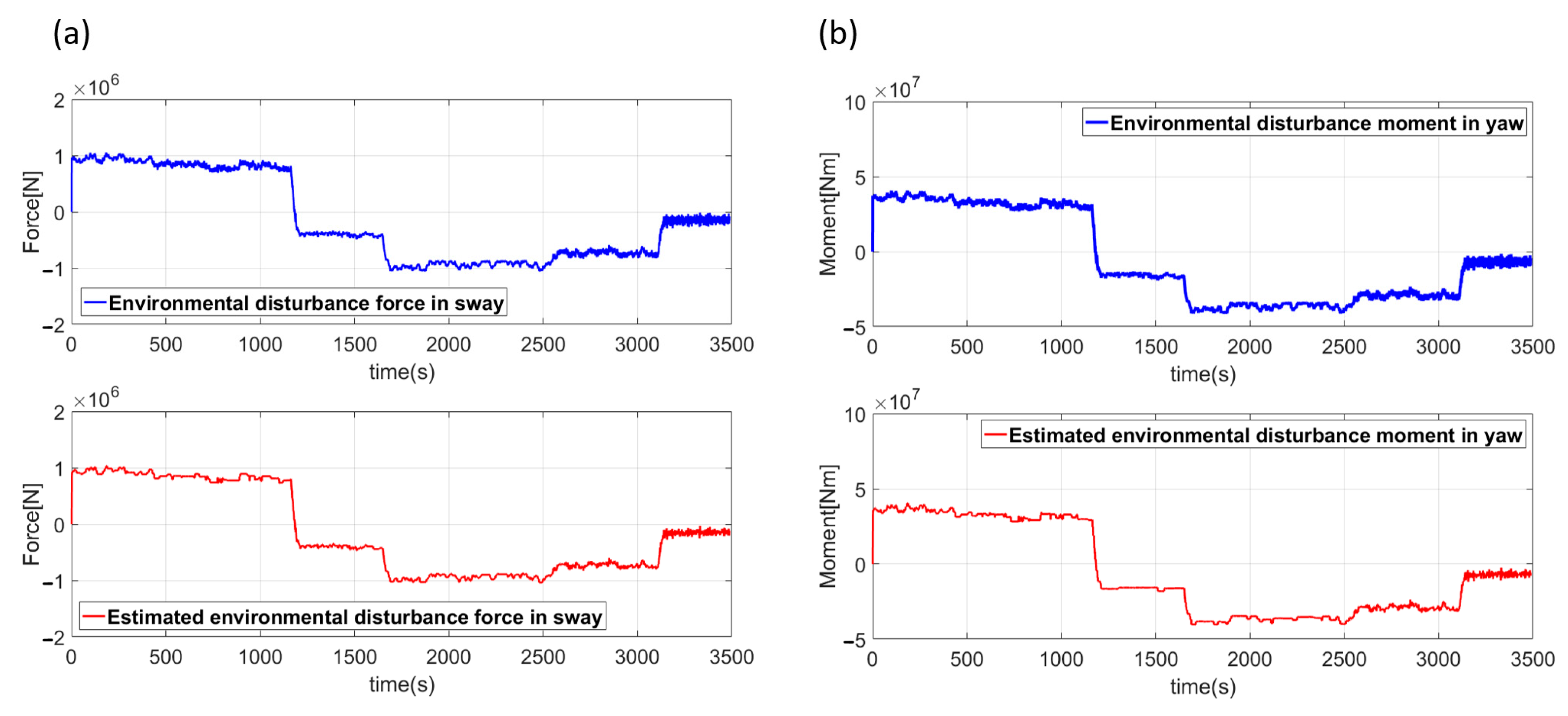
Because environmental disturbances affect the surge, sway, and yaw of the vessel, the magnitude of environmental disturbances must be estimated for these three factors [70]. In Figure 23 and Figure 24, the blue line shows the force and moment added to the vessel by ocean current, wave, and wind; the red line shows the estimated force and moment of the environmental disturbance using the fuzzy disturbance estimator.

The simulation results confirmed that the fuzzy disturbance estimator can reliably estimate the forces and moments of environmental disturbances. In addition, it can be confirmed that it is able to respond even in the alter course section, in which the force and moment of environment disturbance change rapidly. The reason for this is that the fuzzy disturbance estimator proposed in this study has a variable structure and can change the gain value that can estimate the magnitude of the environmental disturbance in real time.

In order for the vessel to accurately follow without departing from the designated route, it is necessary to convert the reliably estimated force and moment of environmental disturbances into thrust and rudder angle that control the actual vessel. The estimated surge force is converted into the thrust $T_{\widehat{est}}\left(k-1\right)$; the estimated sway force and yaw moment are converted into the rudder angle ${\delta }_{\widehat{est}}\left(k-1\right)$.

6.4.3. Simulation of Route-Following Control

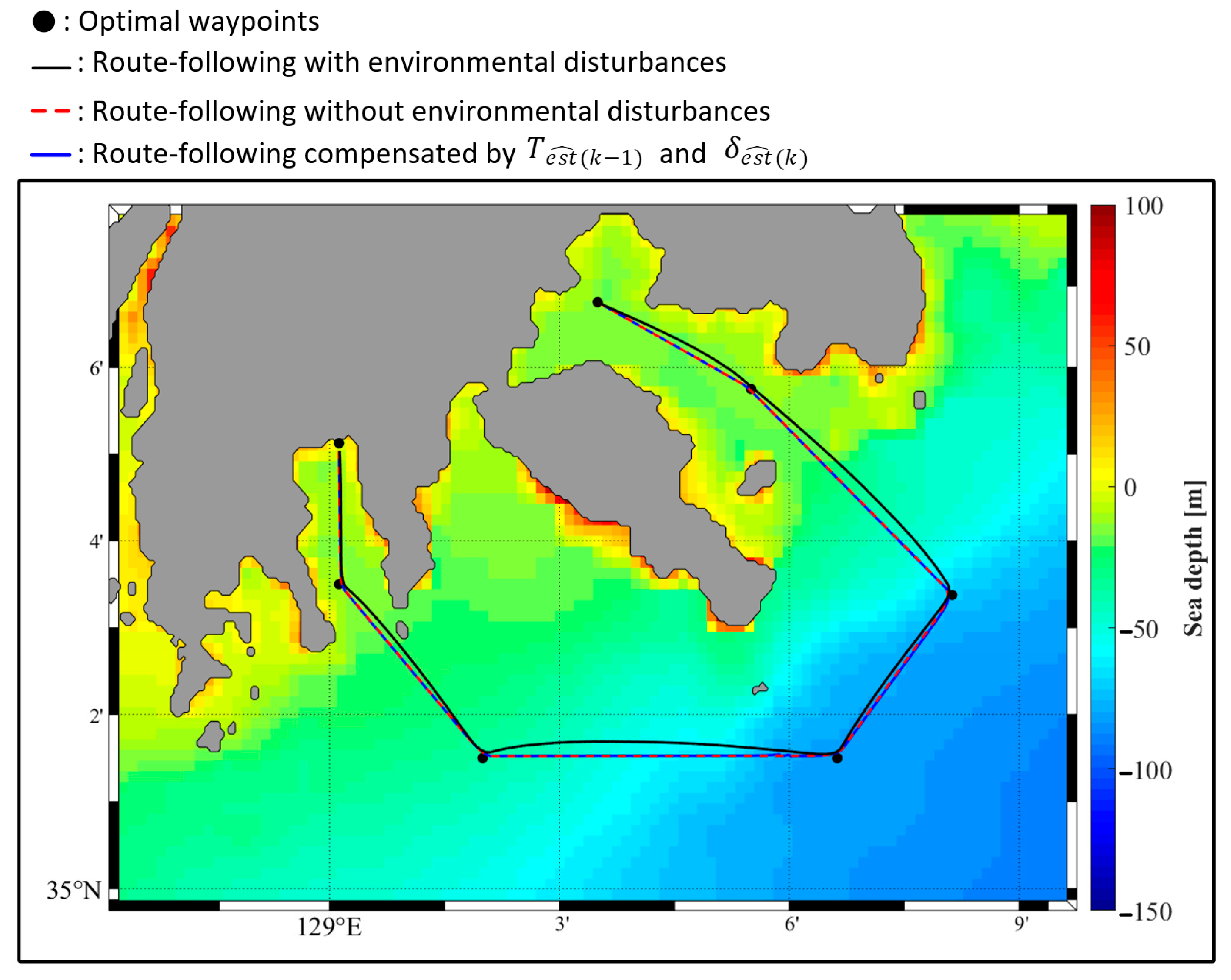
Figure 25 shows the route-following control for cases with and without environmental disturbance, with compensation using $T_{\widehat{est}}\left(k-1\right)$ and ${\delta }_{\widehat{est}}\left(k-1\right)$. The red dotted line shows the result of route-following control for the case without environmental disturbance. The simulation results confirmed that the sufficiently designated route was adequately maintained, even when only the velocity-type fuzzy PID controller was used.

However, when environmental disturbances were applied to the vessel, as indicated by the black solid line in Figure 25, the vessel was not able to accurately follow the designated route; thus, route deviation occurred. This increased the time for the vessel to reach the destination; it also caused economic loss by increasing fuel consumption. Because of this problem, it is necessary to estimate the force and moment of environmental disturbances using a fuzzy disturbance estimator.

The blue solid line shows the simulation result, compensated for using $T_{\widehat{est}}\left(k-1\right)$ and ${\delta }_{\widehat{est}}\left(k-1\right)$ to prevent route deviation because of environmental disturbances. The simulation results confirmed that route-following control was possible without deviating from the route, despite continuous application of environmental disturbances to the vessel.

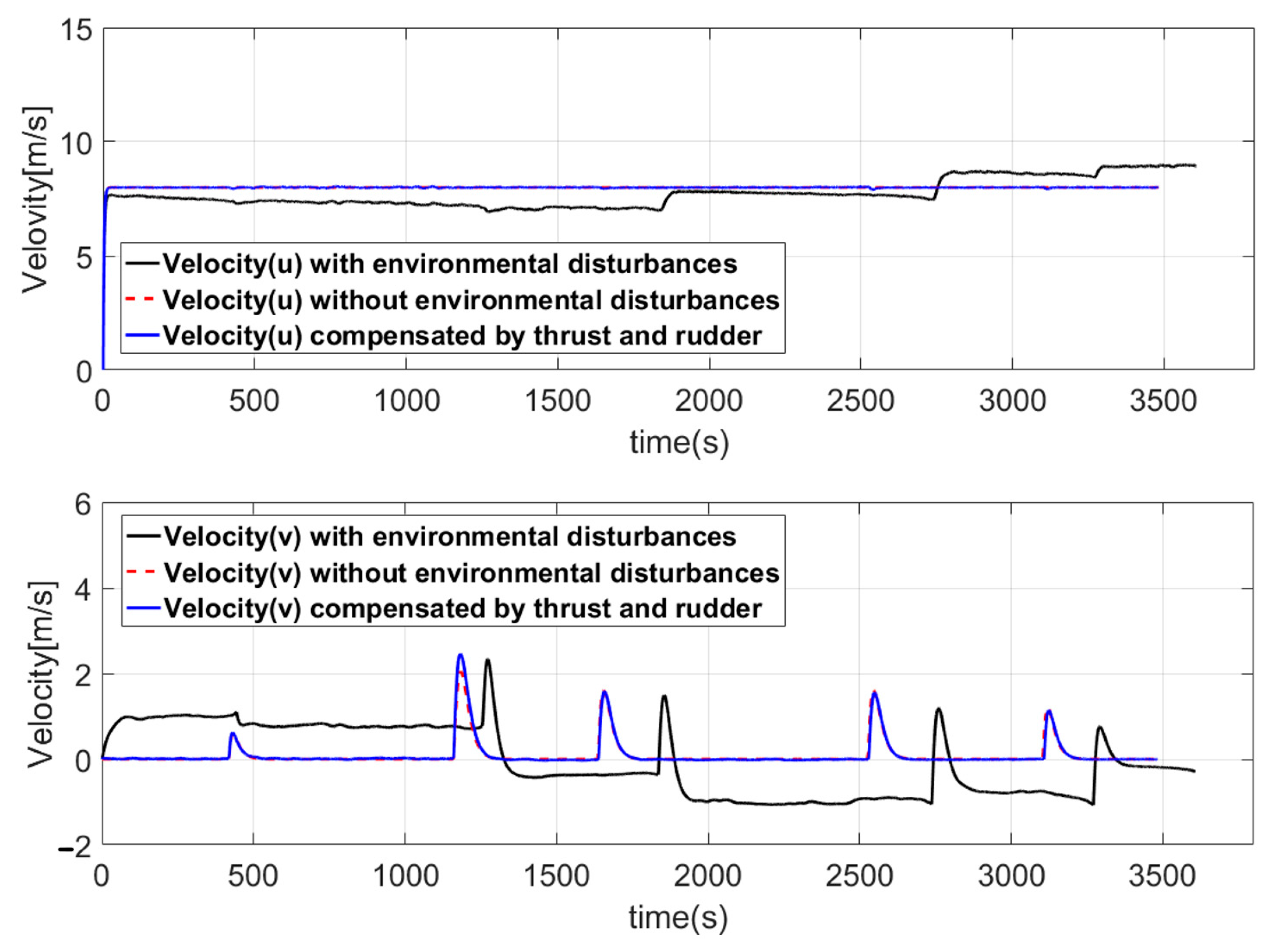
Figure 26 shows the vessel’s velocities. The black solid line is a simulation result showing the vessel velocities after application of environmental disturbances to the vessel; it is clear that velocities increased or decreased according to vessel’s heading angle. The environmental disturbances applied to $u$ simply increased or decreased the forward velocity of the vessel, whereas environmental disturbances applied to $v$ caused the vessel to deviate from the designated route.

However, when the effects of environmental disturbances were compensated for using $T_{\widehat{est}}\left(k-1\right)$ and ${\delta }_{\widehat{est}}\left(k-1\right)$, the velocity $v$ did not occur in the section except for the alter course; thus, the vessel did not deviate from the route. Additionally, the velocity $u$ could be held constant at 8 $\mathrm{m}/\mathrm{s}$. Through such a result, it can be expected that the vessel maintains the set forward velocity at a constant and accurately route-following is possible without deviating from the designated route.

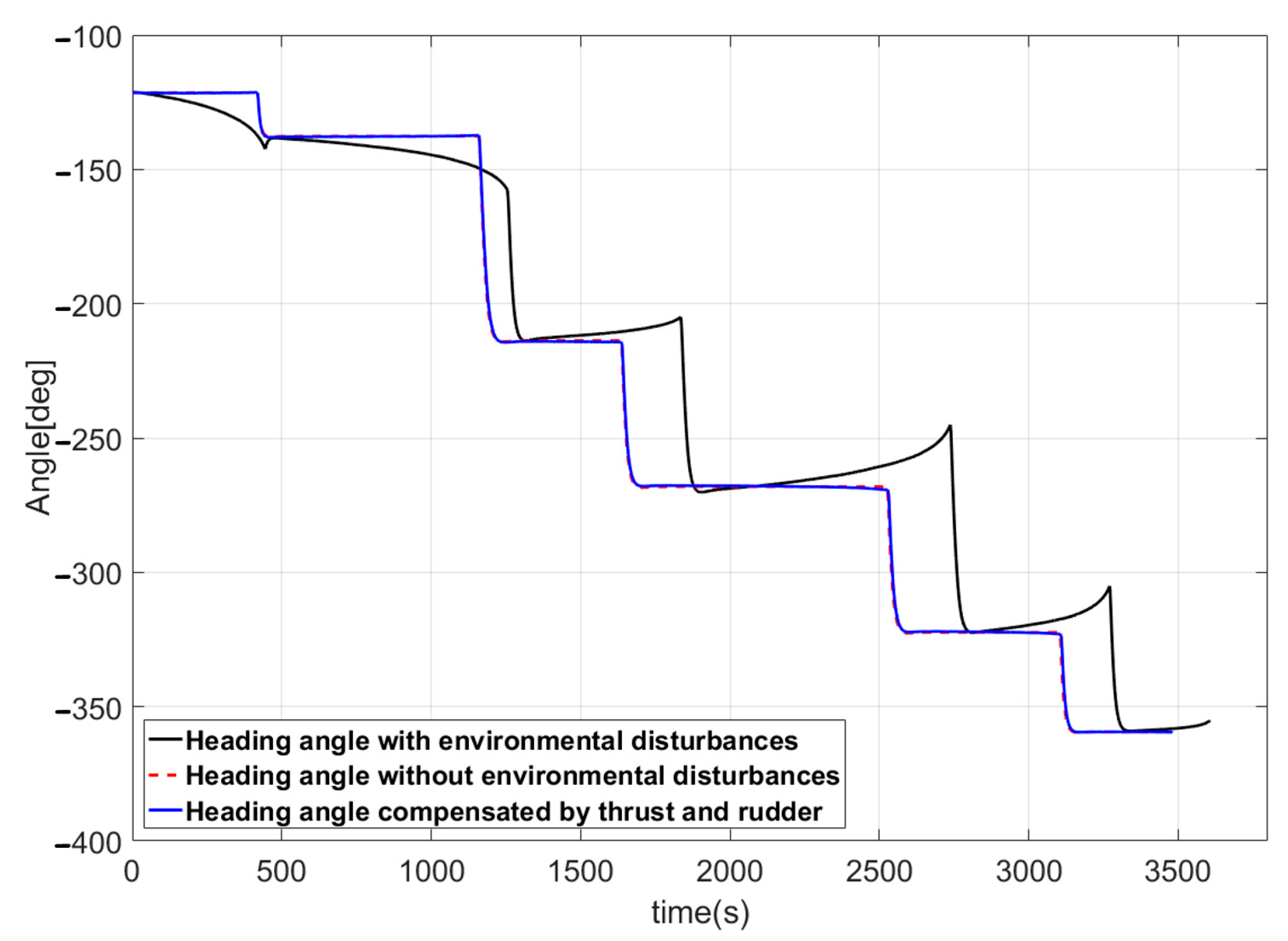
Figure 27 shows the vessel heading angles. As indicated by the solid black line, if environmental disturbances were applied to the vessel, the vessel heading angle could not be maintained constant; it changed continuously, because the heading angle changed in real time due to the rudder being continuously controlled to ensure that the vessel arrived at the next waypoint.

When the environmental disturbances were compensated by $T_{\widehat{est}}\left(k-1\right)$ and ${\delta }_{\widehat{est}}\left(k-1\right)$, the heading angle changed only in the alter course section, and the heading angle remained constant in the other section. This result was similar to the case without environmental disturbances.

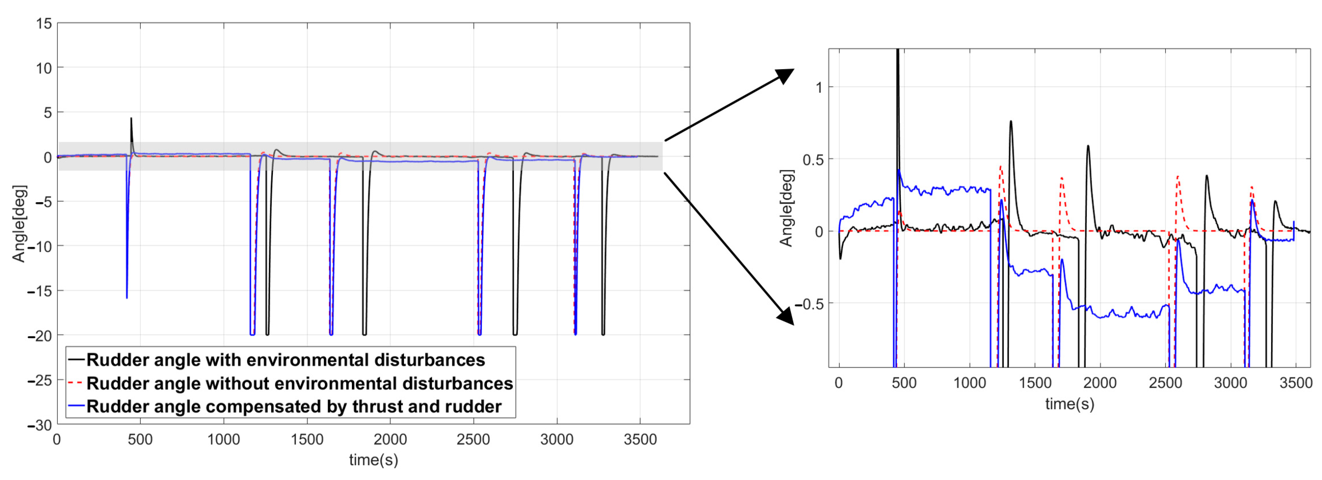
In Figure 25, Figure 26 and Figure 27, the simulation results corresponding to the case without environmental disturbances and the case where compensation was performed using $T_{\widehat{est}}\left(k-1\right)$ and ${\delta }_{\widehat{est}}\left(k-1\right)$ were similar. However, the rudder angle simulation results were different because an additional rudder angle was applied to the vessel to cope with environmental disturbances. Figure 28 shows the rudder angles of the vessel. As indicated by the solid black line, it can be confirmed that a certain angle is generated for the rudder to respond to environmental disturbances. According to the direction and magnitude of the environmental disturbances acting on the vessel, the rudder angle is compensated in $+$ and $-$ directions to an angle suitable for the magnitude.

These simulation results confirmed that the method proposed in this study can accurately follow the designated route, despite the application of environmental disturbances to the vessel.

7. Conclusions

In this study, to satisfy the navigation requirements of autonomous vessels, an optimal route was determined considering both vessel fuel consumption and vessel safety; a route-following control method that could accurately follow the designated route was proposed.

To achieve these requirements, an optimal route was generated based on reinforcement learning, and a velocity-type fuzzy PID controller that could accurately follow the route was introduced. Additionally, to prevent route deviation because of environmental disturbances, a fuzzy disturbance estimator capable of estimating environmental disturbance magnitude was designed. The estimated environmental disturbance magnitudes were converted to the thrust and rudder angle to control the vessel and thus prevent route deviation.

To verify the method proposed in this study, simulations for route-following control were performed using the derived 3 DOF vessel model. The following conclusions were obtained:

(1)

To generate an optimal route, reinforcement learning based on Q-learning algorithms was introduced. The optimal route was generated in a manner that ensured vessel safety and minimized fuel consumption. To ensure safety, under-keel clearance, navigation charts, and sea depth were considered; shortening distance and minimum number of waypoints were considered to minimize fuel consumption. The optimal route from Busan port to Gamcheon port was determined using a traffic separation scheme, restricted area, anchorage, and pilot boarding place. The results of the simulation using the Q-learning algorithm confirmed that the optimal route could be generated while satisfying the requirements.

(2)

For the optimal route generated using the Q-learning algorithm, a route-following control method that can accurately follow the route is required. Conventionally, a PD controller is used to control the vessel, but such a controller has limitations including fast course alterations, rough rudder angle changes, and route deviation related to large overshoot. To resolve these problems, a velocity-type fuzzy PID controller was introduced. Use of the velocity-type fuzzy PID controller did not result in large overshoot; thus, the vessel did not deviate from the designated route. Additionally, because the changes in rudder angle were smooth, the vessel energy efficiency increased.

(3)

Despite the use of a velocity-type fuzzy PID controller, the application of environmental disturbances (ocean current, waves, and wind) to the vessel prevented accurate route-following control. To resolve this problem, a control method capable of following the route without deviation, regardless of environmental disturbances, was proposed. First, the presence or absence of environmental disturbance was determined based on the characteristics of the Kalman filter innovation process; when environmental disturbance was present, the magnitude of the disturbance was estimated using the fuzzy disturbance estimator. Conversion of the magnitude of the estimated environmental disturbance into thrust and rudder angle actually controlling the vessel allowed the designated route to be accurately followed, even in the presence of such environmental disturbances.

The study reported here demonstrated the potential for an autonomous vessel to generate and follow an optimal route by itself, while responding to the effects of environmental disturbance. Further research is needed to implement the proposed optimal route generation algorithm on ECDIS and apply the route-following control technology to actual vessels.

References

1. Statheros, T.; Howells, G.; Maier, K. Autonomous ship collision avoidance navigation concepts, technologies and techniques. J. Navig. 2008, 61, 129–142. [Google Scholar] [CrossRef] [Green Version]
2. Chun, D.H.; Roh, M.I.; Lee, H.W.; Ha, J.; Yu, D. Deep reinforcement learning-based collision avoidance for an autonomous ship. Ocean Eng. 2021, 234, 109216. [Google Scholar] [CrossRef]
3. Guo, S.; Zhang, X.; Zheng, Y.; Du, Y. An autonomous path planning model for unmanned ships based on deep reinforcement learning. Sensors 2020, 20, 426. [Google Scholar] [CrossRef] [Green Version]
4. Batakden, B.M.; Leikanger, P.; Wide, P. Towards autonomous maritime operations. In Proceedings of the IEEE International Conference on Nomputational Intelligence and Virtual Environments for Measurement Systems and Applications, Annecy, France, 26–28 June 2017; pp. 1–6. [Google Scholar]
5. MUNIN. MUNIN Results. 2016. Available online: http://www.unmanned-ship.org/munin/about/munin-results-2 (accessed on 5 January 2016).
6. Chang, C.H.; Kontovas, C.; Yu, Q.; Yang, Z. Risk assessment of the operations of maritime autonomous surface ships. Reliab. Eng. Syst. Saf. 2021, 207, 107324. [Google Scholar] [CrossRef]
7. Goerlandt, F. Maritime autonomous surface ships from a risk governance perspective: Interpretation and implications. Saf. Sci. 2020, 128, 104758. [Google Scholar] [CrossRef]
8. Lewantowica, Z.H. Architectures and GPS/INS integration: Impact on mission accomplish. IEEE Aerosp. Electron. Syst. Mag. 1992, 7, 16–20. [Google Scholar] [CrossRef] [Green Version]
9. Vik, B.; Fossen, T.I. A Nonlinear observer for integration of GPS and inertial navigation systems. Mic J. 2000, 21, 192–208. [Google Scholar] [CrossRef] [Green Version]
10. Lie, C.; Mao, Q.; Chu, X.; Xie, S. An improved A-star algorithm considering water current, traffic separation and berthing for vessel path planning. Appl. Sci. 2019, 9, 1057. [Google Scholar] [CrossRef] [Green Version]
11. Wang, H.; Mao, W.; Eriksson, A. A three-dimensional Dijkstra’s algorithm for multi-objective ship voyage optimization. Ocean Eng. 2019, 186, 106131. [Google Scholar] [CrossRef]
12. Roland, S.B. An intelligent integrated ship guidance system. IFAC Proc. Vol. 1992, 25, 13–25. [Google Scholar]
13. Fang, M.C.; Lin, Y.H.; Wang, B.J. Applying the PD controller on the roll reduction and track keeping for the ship advancing in waves. Ocean Eng. 2012, 54, 13–25. [Google Scholar] [CrossRef]
14. Heidar, A.; Li, M.H.; Chen, G. New design and stability analysis of fuzzy proportional-derivative control systems. IEEE Trans. Fuzzy Syst. 1994, 2, 245–254. [Google Scholar]
15. Cho, K.H.; Kim, C.W.; Lim, J.T. On stability analysis of nonlinear plants with fuzzy logic controllers. In Proceedings of the Korean Institute of Intelligent Systems Conference, Taejon, Republic of Korea, 1 June 1993; pp. 1094–1097. [Google Scholar]
16. Nam, S.K.; Yoo, W.S. Fuzzy PID control with accelerated reasoning for DC servo motors. Eng. Appl. Artif. Intell. 1994, 7, 559–569. [Google Scholar] [CrossRef]
17. He, S.; Tan, S.; Xu, F.; Wang, P. Fuzzy self-tuning of PID controllers. Fuzzy Sets Syst. 1993, 56, 37–46. [Google Scholar] [CrossRef]
18. Ju, J.; Zhang, C.; Liu, Y. Vibration suppression of a flexible-joint robot based on parameter identification and fuzzy PID controller. Algorithms 2018, 11, 189. [Google Scholar] [CrossRef] [Green Version]
19. Huang, H.; Yang, X.Y.; Deng, X.L.; Qiao, Z.H. A parameter auto-tuning method of fuzzy PID controller. Fuzzy Inf. Eng. 2009, 2, 1193–1200. [Google Scholar]
20. Li, Z.; Sun, J. Disturbance compensating model predictive control with application to ship heading control. IEEE Trans. Control Syst. Technol. 2011, 20, 257–265. [Google Scholar] [CrossRef]
21. Zhang, H.L.; Wei, Y.; Hu, X. Anti-disturbance control for dynamic positioning system of ships with disturbances. Appl. Math. Comput. 2021, 396, 125929. [Google Scholar] [CrossRef]
22. Siswantoro, J.; Prabuwono, A.S.; Abdullah, A. A linear model based on Kalman filter for improving neural network classification performance. Expert Syst. Appl. 2016, 49, 112–122. [Google Scholar] [CrossRef]
23. Wierenga, R.D. An evaluation of a pilot model based on Kalman filtering and optimal control. IEEE Trans. Man-Mach. Syst. 1969, 10, 109–117. [Google Scholar] [CrossRef]
24. Soule, A.; Salamatain, K.; Nucci, A.; Taft, N. Traffic matrix tracking using Kalman filter. ACM Sigmatrics Perform. Eval. Rev. 2005, 33, 24–31. [Google Scholar] [CrossRef]
25. Zhen, Y.; Harlim, J. Adaptive error covariance estimation methods for ensemble Kalman filters. J. Comput. Phys. 2015, 294, 619–638. [Google Scholar] [CrossRef] [Green Version]
26. Chen, C.; Chen, X.Q.; Ma, F.; Zeng, X.J.; Wang, J. A knowledge-free path planning approach for smart ships based on reinforcement learning. Ocean Eng. 2019, 189, 106299. [Google Scholar] [CrossRef]
27. Guo, S.; Zhang, X.; Du, Y.; Zheng, Y.; Cao, Z. Path planning of coastal ships based on optimized DQN reward function. Jmse 2021, 9, 210. [Google Scholar] [CrossRef]
28. Guo, S.; Zhang, X.; Zheng, Y.; Du, Y. An autonomous path planning model for unmanned ships based on deep reinforcement learning. Sensors 2020, 20, 426. [Google Scholar] [CrossRef]
29. Shen, H.; Hashimoto, H.; Matsuda, A.; Taniguchi, Y.; Terada, D.; Guo, C. Automatic collision avoidance of multiple ships based on deep Q-learning. Appl. Ocean Res. 2019, 86, 268–288. [Google Scholar] [CrossRef]
30. Zhao, L.; Roh, M.I. COLREGs-compliant multiship collision avoidance based on deep reinforcement learning. Ocean Eng. 2019, 191, 106436. [Google Scholar] [CrossRef]
31. Li, L.; Wu, D.; Huang, Y.; Yuan, Z.M. A path planning strategy unified with a COLREGS collision avoidance function based on deep reinforcement learning and artificial potential field. Appl. Ocean Res. 2021, 113, 102759. [Google Scholar] [CrossRef]
32. Zhao, L.; Roh, M.I.; Lee, S.J. Control method for path following and collision avoidance of autonomous ship based on deep reinforcement learning. J. Mar. Sci. Technol. 2019, 27, 1. [Google Scholar]
33. Nan, G.; Dan, W.; Zhouhua, P.; Jun, W.; Qing, L.H. Advances in line-of-sight guidance for path following of autonomous marine vehicles: An overview. IEEE Trans. Syst. Man Cybern. 2023, 53, 12–28. [Google Scholar]
34. Lili, W.; Yixin, S.; Huajun, Z.; Binghua, S.; Mahmoud, S.A. An improved integral light-of sight guidance law for path following of unmanned surface vehicles. Ocean Eng. 2020, 205, 107302. [Google Scholar]
35. Zhang, Q.; Ding, Z.; Zhang, M. Adaptive self-regulation PID control of course-keeping for ships. Pol. Marit. Res. 2020, 27, 39–45. [Google Scholar] [CrossRef]
36. Wang, L.; Wu, Q.; Liu, J.; Li, S.; Negenborn, R.R. State-of-the-art research on motion control of maritime autonomous surface ships. J. Mar. Sci. Eng. 2019, 7, 438. [Google Scholar] [CrossRef] [Green Version]
37. Le, T.T. Ship heading control system using neural network. J. Mar. Sci. Technol. 2021, 26, 963–972. [Google Scholar] [CrossRef]
38. Wang, L.; Xu, H.; Zou, U. Regular unknown input functional observers for 2-D singular systems. Int. J. Control Autom. Syst. 2013, 11, 911–918. [Google Scholar] [CrossRef]
39. Lee, M.K. Unknown input estimation of the linear systems using integral observer. J. Korean Inst. Illum. Electr. Install. Eng. 2008, 22, 101–106. [Google Scholar]
40. Youssef, T.; Chadli, M.; Karimi, H.R.; Wang, R. Actuator and sensor faults estimation based on proportional integral observer for TS fuzzy model. J. Frankl. Inst. 2017, 354, 2524–2542. [Google Scholar] [CrossRef]
41. Witczak, M.; Kornicz, J.; Jozefowicz, R. Design of unknown input observers for non-linear stochastic systems and their application to robust fault diagnosis. Control Cybern. 2013, 42, 227–256. [Google Scholar]
42. Lee, K.K.; Ha, W.S.; Back, J.H. Overview of disturbance observation techniques for linear and nonlinear systems. J. Inst. Control Robot. Syst. 2016, 22, 332–338. [Google Scholar] [CrossRef]
43. Kwak, G.; Park, S. State space disturbance observer considering sliding mode and robustness improvement for mismatched disturbance. J. Inst. Control Robot. Syst. 2021, 27, 639–645. [Google Scholar] [CrossRef]
44. Zhao, Z.; Cao, D.; Yang, J.; Wang, H. High-order sliding mode observer-based trajectory tracking control for a quadrotor UAV with uncertain dynamics. Nonlinear Dyn. 2020, 102, 2583–2596. [Google Scholar] [CrossRef]
45. Kim, M.K.; Park, D.H.; Oh, Y.W.; Kim, J.H.; Choi, J.K. Towfish attitude control: A consideration of towing point, center of gravity, and towing speed. J. Mar. Sci. Eng. 2021, 9, 641. [Google Scholar] [CrossRef]
46. Fossen, T.I. Handbook of Marine Craft Hydrodynamics and Motion Control; John Willy & Sons LTD: Sussex, UK, 2011. [Google Scholar]
47. Blanke, M. Ship Propulsion Losses Related to Automated Steering and Prime Mover Control. Ph.D. Thesis, The Technical University of Denmark, Kongens Lyngby, Denmark, 1981. [Google Scholar]
48. Davidson, K.S.M.; Schiff, L.I. Turning and Course Keeping Qualities Transactions of SNAME; Report number T1946-1/SNAME; Marine and Transport Technology: Delft, The Netherlands, 1946. [Google Scholar]
49. Fossen, T.I. Marine Control System; Marine Cybermetics: Trondheim, Norway, 2002. [Google Scholar]
50. Kim, M.K.; Yang, H.; Kim, J.H. Improvement of ship’s DP system performance using control increment of velocity type fuzzy PID controller. J. Korean Soc. Mar. Eng. 2019, 43, 40–47. [Google Scholar]
51. Dayan, P.; Niv, Y. Reinforcement learning: The good, the bad and the ugly. Curr. Opin. Neurobiol. 2008, 18, 185–196. [Google Scholar] [CrossRef]
52. Bae, H.; Kim, G.; Kim, J.; Qian, D.; Lee, S. Multi-robot path planning method using reinforcement learning. Appl. Sci. 2019, 9, 3057. [Google Scholar] [CrossRef] [Green Version]
53. Maoudj, A.; Hentout, A. Optimal path planning approach based on Q-learning algorithm for mobile robots. Appl. Soft Comput. 2020, 97, 106796. [Google Scholar] [CrossRef]
54. Yan, C.; Xiang, X. A path planning algorithm for UAV based on improved Q-learning. In Proceedings of the 2018 2th International Conference on Robotics and Automation Science 2018, Wuhan, China, 23–25 June 2018; pp. 1–5. [Google Scholar]
55. Lee, W.; Yoo, W.; Choi, G.H.; Ham, S.H.; Kim, T.W. Determination of optimal ship route in coastal sea considering sea state and under keel clearance. J. Soc. Nav. Archit. Korea 2019, 56, 480–487. [Google Scholar] [CrossRef]
56. Kim, J.H.; Oh, S.J. A fuzzy PID controller for nonlinear and uncertain systems. Soft Comput. 2000, 4, 123–129. [Google Scholar] [CrossRef]
57. Long, Z.; Yuan, Y.; Long, W. Designing fuzzy controllers with variable universes of discourse using input-output data. Eng. Appl. Artif. Intell. 2014, 36, 215–221. [Google Scholar] [CrossRef]
58. Hu, Y.; Yang, Y.; Li, S.; Zhou, Y. Fuzzy controller design of micro-unmanned helicopter relying on improved genetic optimization algorithm. Aerosp. Sci. Technol. 2020, 98, 105685. [Google Scholar] [CrossRef]
59. Zhu, Z.; Liu, Y.; He, Y.; Wu, W.; Wang, H.; Huang, C.; Ye, B. Fuzzy PID control of the three-degree-of-freedom parallel mechanism based on genetic algorithm. Appl. Sci. 2022, 12, 11128. [Google Scholar] [CrossRef]
60. Sumar, R.R.; Coelho, A.A.R.; Coelho, L.D.S. Computational intelligence approach to PID controller design using the universal model. Inf. Sci. 2010, 180, 3980–3991. [Google Scholar] [CrossRef]
61. Kim, Y.H.; Ahn, S.C.; Kwon, W.H. Computational complexity of general fuzzy logic control and its simplification for a loop controller. Fuzzy Sets Syst. 2000, 111, 215–224. [Google Scholar] [CrossRef]
62. Peters, L.; Guo, S.; Camposano, R. A novel analog fizzy controller for intelligent sensors. Fuzzy Sets Syst. 1995, 70, 235–247. [Google Scholar] [CrossRef]
63. Dumitrescu, C.; Ciotirnae, P.; Vizitiu, C. Fuzzy logic for intelligent control system using soft computing applications. Sensors 2021, 21, 2617. [Google Scholar] [CrossRef] [PubMed]
64. Kwak, S.; Choi, B.J. Deffuzzification scheme and its numerical example for fuzzy logic based control system. J. Korea Inst. Intell. Syst. 2018, 28, 350–354. [Google Scholar]
65. Kim, J.H.; Ha, Y.S.; Lim, J.K.; Seo, S.K. A suggestion of fuzzy estimation technique for uncertainty estimation of linear time invariant system based on Kalman filter. J. Korea Soc. Mar. Eng. 2012, 36, 919–926. [Google Scholar] [CrossRef]
66. Kim, D.; Lee, S.M.; Jung, S.; Koo, J.; Myung, H. Particle swarm optimization-based receding horizon formation control of multi-agent surface vehicle. Adv. Robot. Res. 2018, 2, 161–182. [Google Scholar]
67. Chen, X.; Zhou, L.; Zhou, M.; Shao, A.; Ren, K.; Chen, Q.; Gu, G.; Wan, M. Infrared ocean image simulation algorithm based on pierson-moskowitz spectrum and bidirectional reflectance distribution function. Photonics 2022, 9, 166. [Google Scholar] [CrossRef]
68. Berge, S.P.; Ohtsu, K.; Fossen, T.I. Nonlinear control of ships minimizing the position tracking errors. Model. Identif. Control 1999, 20, 177–189. [Google Scholar] [CrossRef] [Green Version]
69. Isherwood, R.W. Wind resistance of merchant ships. RINA Trans. 1972, 115, 327–338. [Google Scholar]
70. Kim, M.K. A Study on Generation of Optimal Route and Route following Control for Autonomous Vessel. Ph.D. Dissertation, Korea Maritime & Ocean University, Busan, Republic of Korea, February 2023. [Google Scholar]
Figure 1. Definitions of earth-fixed and body-fixed coordinate systems.
Jmse 11 00970 g001
Figure 2. Vessel used in this study.
Jmse 11 00970 g002
Figure 3. Definition of reinforcement learning.
Jmse 11 00970 g003
Figure 4. Types of reinforcement-learning algorithms according to learning method.
Jmse 11 00970 g004
Figure 5. Definitions of eight directions in which the agent can take action.
Jmse 11 00970 g005
Figure 6. Concept of the Q-learning algorithm.
Jmse 11 00970 g006
Figure 7. Definition of the optimal route.
Jmse 11 00970 g007
Figure 8. Algorithm to satisfy minimum fuel consumption.
Jmse 11 00970 g008
Figure 9. Integrated environment for optimal route generation.
Jmse 11 00970 g009
Figure 10. Optimal route generated by Q-learning algorithm and Douglas–Peucker algorithm.
Jmse 11 00970 g010
Figure 11. Optimal route generated by the Q-learning and Douglas–Peucker algorithms.
Jmse 11 00970 g011
Figure 12. Performance comparison with A * algorithm.
Jmse 11 00970 g012
Figure 13. Structure of the velocity-type fuzzy PID controller.
Jmse 11 00970 g013
Figure 14. Fuzzification algorithm for inputs and outputs. (a) Fuzzification algorithm for ψ e * , ψ r * and ψ a * . (b) Fuzzification algorithm for d δ 1 k . (c) Fuzzification algorithm for d δ 2 k .
Jmse 11 00970 g014
Figure 15. Input combinations for fuzzy control blocks 1 and 2. (a) Input combinations for ψ e * , ψ r * . (b) Input combinations for ψ r * , ψ a * .
Jmse 11 00970 g015
Figure 16. Results of route-following using the PD and velocity-type fuzzy PID controllers.
Jmse 11 00970 g016
Figure 17. Results of velocities u and v using the PD and velocity-type fuzzy PID controllers.
Jmse 11 00970 g017
Figure 18. Results of headings using the PD and velocity-type fuzzy PID controllers.
Jmse 11 00970 g018
Figure 19. Results of rudder angles using the PD and velocity-type fuzzy PID controllers.
Jmse 11 00970 g019
Figure 20. Determination of the existence of environmental disturbances.
Jmse 11 00970 g020
Figure 21. Structure of the fuzzy disturbance estimator.
Jmse 11 00970 g021
Figure 22. Block diagram of the route-following control system to eliminate the effects of environmental disturbance.
Jmse 11 00970 g022
Figure 23. Estimation of environmental disturbance force in surge.
Jmse 11 00970 g023
Figure 24. Estimation of environmental disturbance force in (a) sway and (b) moment in yaw.
Jmse 11 00970 g024
Figure 25. Route-following control for the cases with and without environmental disturbance, with compensation using T e s t ^ k 1 and δ e s t ^ k 1 .
Jmse 11 00970 g025
Figure 26. Velocities u and v for the case with or without environmental disturbance, and compensated for using T e s t ^ k 1 and δ e s t ^ k 1 .
Jmse 11 00970 g026
Figure 27. Heading angles for the case with or without environmental disturbance, and compensated for using T e s t ^ k 1 and δ e s t ^ k 1 .
Jmse 11 00970 g027
Figure 28. Rudder angles for the case with or without environmental disturbance and compensated for using T e s t ^ k 1 and δ e s t ^ k 1 .
Jmse 11 00970 g028