Intervehicle Security-Based Robust Neural Formation Control for Multiple USVs via APS Guidance

Abstract

This paper focuses on the intervehicle security-based robust formation control of unmanned surface vehicles (USVs) to implement the formation switch mission. In the scheme, a novel adaptive potential ship (APS)-based guidance principle is developed to prevent intervehicle collisions, which is common and threatening when maneuvering a formation switch. By employing the artificial potential field (APF), the APS can program the real-time attitude reference for USVs by using the security intervehicle distance while achieving the path-following task. As for the control part, a robust adaptive formation control algorithm is proposed to effectively stabilize the USVs to the APS via the fusion of the disturbance observer (DOB) and by using the robust neural damping technique. Regarding the merits of the improved design of the DOB, the weight compression of the neural networks can effectively simplify the structure of the DOB and enhance the observation accuracy of the external disturbance. This can facilitate the avoidance of intervehicle collisions and guarantee the application of the theoretical algorithm in engineering practice. Considerable effort has been made to obtain the semiglobally uniform ultimate bounded (SGUUB) stability via theoretical analysis. Finally, with the sailing scene in a narrow channel, the simulated experiment is illustrated to verify the security performance of the proposed strategy.

1. Introduction

In the past few decades, multiple unmanned surface vehicles (USVs) have drawn intense attention because of their good maneuverability, exceptional versatility and low cost. Building on different formation guidance principles, e.g., a leader–follower approach [1], topology-based approach [2], virtual structure approach [3], behavioral-based approach [4] and so on, USV formation control has been studied actively, and the study of formation tracking has made significant progress [5,6]. However, in marine practice, it is unpractical for USVs to maintain an unchanged formation structure due to different navigation scenarios. Therefore, the switch of the USV formation has attracted more and more attention.

The switch of the USV formation is widespread in practical applications, e.g., cooperative transportation, channel crossing, the formation avoidance of obstacles, etc. Generally, graph theory is a popular method to deal with multiagent tracking control problems [7]. Additionally, a topology-based formation is more flexible than a leader–follower approach in terms of a formation switch. In [8], the USV formation shape was changed by switching the topology and applying a distributed nonlinear model predictive control (NMPC) solution. In [9], a flexible multigroup adaptive time-varying formation algorithm was presented on the basis of graph theory. In [10], a group of underactuated ships with a shrunk pentagon formation was demonstrated based on the undirected graph. Furthermore, a multi-USV system under swarm center position (SCP) guidance and an improved artificial potential field (APF) achieved a formation switch while avoiding a collision with obstacles in [11]. By utilizing model predictive control (MPC) and the alternating direction of multipliers method (ADMM), three autonomous surface vessels (ASVs) used for cooperative transportation performed formation transitioning and obstacle avoidance in [12]. In the above studies, topology and MPC were used to solve the formation switch problems, while the leader–follower approach was neglected. Though the leader–follower approach is less flexible, it is a simpler and more visualized method. Taking full advantage of the leader–follower approach and developing an improved leader–follower method that is suitable for formation switch problems is necessary.

Typically, the leader–follower method for USV formation navigation is functionally divided into two parts: guidance and control. Regarding the traditional leader–follower guidance principle, followers are supposed to track the leader with a certain position and orientation errors [13,14]. As for the traditional leader–follower approach, intervehicle communication is the most serious challenge when dealing with a formation switch. By switching the distance between the leader and followers, the USVs performed a formation shrinking task in [15]. Obviously, the traditional leader–follower approach is not flexible, and it is only resultful for a small-range formation switch. Thus, designing an extra guidance program is vital to guide USVs toward the switched formation. Still, intervehicle collision avoidance is a significant problem in terms of formation switches, which require USVs to share their kinematic data with each other. The briefest method for avoiding collisions is using the APF, which is a real-time obstacle avoidance approach affected by virtual forces [16]. The basic idea of an APF is to vividly abstract the environment as two different artificial force fields, which are attractive potential fields and repulsive potential fields. In the collision-avoidance scenario, the target generates an attractive potential field, while obstacles generate repulsive potential fields. The robot is inevitably affected by those artificial force fields composed of attractive force and repulsive forces. As a result, the robot is able to track the target and avoid obstacles. Because of the profit from its concision and strong logic, APFs have been widely employed in USV research fields. A real-time guidance principle based on an improved APF and dynamic virtual ship (DVS) for USVs was developed to track targets and avoid obstacles in [17].

As for the control part, the robust neural damping technique based on the neural networks (NNs) technique and minimal learning parameters (MLP) technique was highly used [18,19,20,21]. The NNs approximation technique and MLP technique can be used to deal with the unknown nonlinear terms reasonably and reduce the number of parameters efficiently. However, to improve the control accuracy ulteriorly, a better control algorithm against disturbances is necessary. Ordinarily, there are two main methods used against disturbances, namely stabilizing disturbances [5] and estimating disturbances [22]. A disturbance observer (DOB) was introduced to estimate the disturbances in ship-path-following control in [23]. On the basis of [23], a DOB used to estimate the unknown time-varying disturbances was extended in a ship dynamic positioning task [24]. In [25], a new NNs-based DOB was developed for autonomous surface vessels (ASVs) formation control. Compared with former DOBs, the NNs-based DOB is combined with the robust neural damping technique. The controller and DOB can share the same NNs to transform unknown disturbance items to known estimation items. Such a design contributes to a simpler and more concise structure in controller design.

Motivated by the aforementioned discussion, a novel intervehicle security-based formation control strategy is proposed for USVs to carry out waypoints-based formation keeping and switching. The main contributions of this paper can be summarized as the following two aspects:

(1)

A novel adaptive potential ship (APS)-based guidance principle is developed to implement the real-time path planning of formation keeping and switching, whereby the intervehicle security can be guaranteed in the meantime. In this principle, the leader and followers are all assigned as guidance virtual ships (GVSs) to generate the references for USVs. Regarding the operation of the formation switch, the formation structure of the GVS would be transformed. By employing the APF method, the APSs can be derived according to the relative attitudes of USV-GVS and USV-USV, which always guide USVs toward the reference of GVSs. Different from the existing results, the proposed guidance can make the leader–follower formation a flexible structure. Thus, the APS guidance provides a new method to deal with the formation switch and intervehicle security problem.

(2)

In order to lower the energy consumption, this paper focuses on the precise estimation of marine environment disturbances. A robust adaptive formation control algorithm with a NNs-based DOB is proposed. By estimating the disturbances, the USV is able to distribute outputs as the variation in the marine environment. Compared with the former DOB, the NNs-based DOB requires fewer model parameters’ data information to estimate the disturbances. Different from [10,25], the observational objects in this paper are much more complex and disordered. The disturbances in nautical practice are illustrated to verify the feasibility of the NNs-based DOB.

Specifically, the main content of this paper can be divided into four parts. Useful lemmas and basic knowledge about USV formation are cushioned in Section 2 for subsequent studies. An original guidance strategy for formation keeping and switching along with intervehicle collision avoidance is introduced in Section 3. To further enhance the safety of intervehicle navigation, Section 4 provides a control algorithm with a higher accuracy. Additionally, a numerical simulation is illustrated to verify the performance of the proposed strategy in Section 5.

2. Problem for Formulation and Preliminaries

2.1. USV Formation Modeling

Consider a fleet of $n$ USVs with $n$ APSs and $n$ GVSs; USVs are driven by propellers for surge motions and rudders for yaw motions. The surge motion, sway motion and yaw motion are the most influential motions when it comes to formation-tracking issues. So, based on the Newtonian and Lagrangian mechanics [26], a 3-degrees-of-freedom (3DOF) nonlinear kinematic model of each USV can be established as Equations (1) and (2):

$$\left\{\begin{array}{l}{\dot{x}}_i=u_i\cos \left({\psi }_i\right)-v_i\sin \left({\psi }_i\right)\\ {\dot{y}}_i=u_i\sin \left({\psi }_i\right)+v_i\cos \left({\psi }_i\right)\\ {\dot{\psi }}_i=r_i\end{array}\right.$$

(1)

$$\left\{\begin{array}{l}{\dot{u}}_i=\frac{m_{vi}}{m_{ui}}{v}_i{r}_i-f_{ui}\left(u_i\right)+\frac{{\tau }_{ui}}{m_{ui}}+d_{wui}\\ {\dot{v}}_i=-\frac{m_{ui}}{m_{vi}}{u}_i{r}_i-f_{vi}\left(v_i\right)+d_{wvi}\\ {\dot{r}}_i=\frac{m_{ui}-m_{vi}}{m_{ri}}{u}_i{v}_i-f_{ri}\left(r_i\right)+\frac{{\tau }_{ri}}{m_{ri}}+d_{wri}\end{array}\right.$$

(2)

where ${\eta }_i={\left[x_i,y_i,{\psi }_i\right]}^{\mathrm{T}}\in {ℝ}^3$ denotes the surge, sway displacement and yaw angle in the earth-fixed coordinate, respectively. $v_i={\left[u_i,v_i,r_i\right]}^{\mathrm{T}}\in {ℝ}^3$ describes the surge, sway and yaw velocities in the body coordinate system, respectively. ${\tau }_{ui},{\tau }_{ri}$ indicate the inputs of the control system: the surge force and yaw moment, respectively. $d_{wui},d_{wvi},d_{wri}$ are the unmeasurable environment disturbance forces or moments caused by the wind, waves and ocean current, respectively. $m_{ui},m_{vi},m_{ri},d_{ui},d_{vi},d_{ri},d_{u2i},d_{v2i},d_{r2i},d_{u3i},d_{v3i},d_{r3i}$ are all considered as unknown parameters, and they describe the ships’ inertia, hydrodynamic damping and nonlinear damping terms. The nonlinear functions $f_{ui}\left(u_i\right),f_{vi}\left(v_i\right),f_{ri}\left(r_i\right)$ denote the high-order hydrodynamic effect as outlined in Equation (3):

$$\begin{array}{l}{f}_{ui}\left(u_i\right)=\frac{d_{ui}}{m_{ui}}{u}_i+\frac{d_{u2i}}{m_{ui}}\left|u_i\right|u_i+\frac{d_{u3i}}{m_{ui}}{u}_i^3\\ f_{vi}\left(v_i\right)=\frac{d_{vi}}{m_{vi}}{u}_i+\frac{d_{v2i}}{m_{vi}}\left|v_i\right|v_i+\frac{d_{v3i}}{m_{vi}}{v}_i^3\\ f_{ri}\left(r_i\right)=\frac{d_{ri}}{m_{ri}}{u}_i+\frac{d_{r2i}}{m_{ri}}\left|r_i\right|r_i+\frac{d_{r3i}}{m_{ri}}{r}_i^3\end{array}$$

(3)

Assumption 1.

It is assumed that the environment disturbance terms satisfy $\left|d_{wui}\right|\le {\overline{d}}_{wui}$,  $\left|d_{wvi}\right|\le {\overline{d}}_{wvi}$,  $\left|d_{wri}\right|\le {\overline{d}}_{wri}$, where  ${\overline{d}}_{wui}$,  ${\overline{d}}_{wvi}$,  ${\overline{d}}_{wri}$ are all the positive unknown constants. ${\dot{d}}_{wui}$,  ${\dot{d}}_{wvi}$,  ${\dot{d}}_{wri}$ are all the continuous bounded functions satisfying $\left|{\dot{d}}_{wui}\right|\le C_{ui}$,  $\left|{\dot{d}}_{wvi}\right|\le C_{vi}$,  $\left|{\dot{d}}_{wri}\right|\le C_{ri}$.

Assumption 2.

According to the description in [27], the sway velocity $v_i$ is passive bounded for USVs.

The objective of this paper is to design a formation guidance strategy and a formation adaptive controller for $n$ USVs with Equations (1)–(3) such that the USVs converge to a safe and efficient reference path while achieving the formation switch along the reference path.

Lemma 1.

The following inequality is established for any $\delta >0$ and any $\varrho \in ℝ$ [28].

$$0\le \left|\varrho \right|-\varrho \tan \mathrm{h}\left(\frac{\varrho }{\delta }\right)\le 0.2785\delta$$

(4)

2.2. RBF-NNs

The radial basis function neural networks (RBF-NNs) are efficient and concise tools that can be used to model nonlinear functions, and they have good capabilities in terms of approximating unknown functions [18]. In this paper, the RBF-NNs approximator is used to deal with the uncertain nonlinear terms of the USV kinematic model, and the approximated unknown nonlinear terms are available for weight compression. Therefore, a useful lemma is introduced for later control design.

Lemma 2.

For any given real continuous function $f\left(x\right)$ with $f\left(0\right)=0$, defined in a compact set ${\mathsf{\Omega }}_x\in {ℝ}^m$, when the RBF-NNs approximator and the continuous function separation technique are used, it can always be approximated as follows [29]:

$$f\left(x\right)=A^{\mathrm{T}}S\left(x\right)+\epsilon \left(x\right), \forall x\in {\mathsf{\Omega }}_x$$

(5)

where $A^{\mathrm{T}}={\left[a_1,a_2,\dots ,a_l\right]}^{\mathrm{T}}$ donates the adaptable weight vector, $S\left(x\right)={\left[s_1\left(x\right),s_2\left(x\right),\dots ,s_l\left(x\right)\right]}^{\mathrm{T}}$ is a vector of RBF with the form of Gaussian function Equation (10) and $\epsilon \left(x\right)$ is the approximation error constant with an unknown upper bound $\overline{\epsilon }\left(x\right)$.

$$s_i\left(x\right)=\frac{1}{\sqrt{2\pi }{h}_i}\exp \left(-\frac{{\left(x-{\mu }_i\right)}^{\mathrm{T}}\left(x-{\mu }_i\right)}{2h_i^2}\right), i=1,2,\dots ,l$$

(6)

where $l>1$ is the node number of NNs, ${\mu }_i$ denotes the center of receptive field and $h_i$ indicates the width of the Gaussian function.

3. APS-Based Guidance Principle with Intervehicle Security

To achieve the formation switch and guarantee the intervehicle security, the APS guidance is designed in this section. There are two layers in the proposed guidance principle: the GVS guidance and the APS guidance. According to the waypoints-based reference path, the GVS guidance is designed to program the desired formation structure and the reference path. Regarding APS guidance, the APSs are developed to generate APS reference paths for USVs converging to their corresponding GVSs and to prevent the USVs from colliding with each other.

3.1. The Basis Framework of Guidance Principle

In this paper, GVSs are divided into a GVS-leader and $n-1$ GVS-followers, whereby ${\eta }_1={\left[x_{r1},y_{r1},{\psi }_{r1}\right]}^{\mathrm{T}}$ is defined as the position vector of the GVS-leader and $v_1={\left[u_r,v_r,r_r\right]}^{\mathrm{T}}$ is defined as the velocities vector of the GVS-leader. GVS-followers are generated by a GVS-leader with certain angles and distances between the GVS-leader and GVS-followers; see Figure 1. The distances between the GVS-leader and GVS-followers’ position vectors can be formulated as Equations (7) and (8):

$${\rho }_i=\sqrt{{\left(x_{r1}-x_{ri}\right)}^2+{\left(y_{r1}-y_{ri}\right)}^2}$$

(7)

$${\eta }_i={\eta }_1+R\left({\psi }_{r1}\right){\iota }_i$$

(8)

with

$$R\left({\psi }_{r1}\right)=\left[\begin{array}{ccc}\cos {\psi }_{r1}& -\sin {\psi }_{r1}& 0\\ \sin {\psi }_{r1}& \cos {\psi }_{r1}& 0\\ 0& 0& 1\end{array}\right]$$

(9)

$${\iota }_i=\left[\begin{array}{c}{\rho }_i\cos {\lambda }_i\\ {\rho }_i\cos {\lambda }_i\\ 0\end{array}\right]$$

(10)

where ${\rho }_i$ and ${\lambda }_i$ are the distances and angle between the GVS-leader and GVS-followers, respectively, while ${\eta }_i={\left[x_{ri},y_{ri},{\psi }_{ri}\right]}^{\mathrm{T}}$ donates the position vectors of the GVS-followers. $R\left({\psi }_{r1}\right)$ is the rotation matrix of the GVS-leader, and ${\iota }_i$ denotes the offsets from the GVS-leader to GVS-followers.

In marine practice, the reference path is often generated by the waypoints $W_1,W_2,\dots ,W_n$ with $W_i=\left(x_i,y_i\right)$, which guide the real ship sailing on the open sea [30]. The waypoints-based reference path is made up of straight lines. So, a GVS-leader in the form of Equation (11) could automatically follow the waypoints-based reference path with a desired speed under the GVS guidance, and generating a GVS reference path is required:

$$\left\{\begin{array}{l}{\dot{x}}_{r1}=u_r\cos {\psi }_{r1}\\ {\dot{y}}_{r1}=u_r\sin {\psi }_{r1}\\ {\dot{\psi }}_{r1}=r_r\end{array}\right.$$

(11)

$${\varphi }_{i-1,i}=\arctan \left(\frac{y_i-y_{i-1}}{x_i-x_{i-1}}\right)$$

(12)

$$R_i=\left\{\begin{array}{l}{R}_{\max },\left|\Delta {\varphi }_i\right|\ge \pi /2\hfill \\ \frac{\left(R_{\max }-R_{\min }\right)\Delta {\varphi }_i}{\mathrm{sgn}\left(\Delta {\varphi }_i\right)\pi /2},\left|\Delta {\varphi }_i\right|<\pi /2\hfill \end{array}\right.$$

(13)

Figure 1 presents the basic principle for generating a GVS reference path by a GVS-leader. The GVS reference path is $W_{i-1}{P}_{inWi}\to ar{c}_{Wi}\to P_{outWi}{W}_{i+1}$. Typically, the surge speed ($u_r$) is a positive constant determined by the ship operator or based on the estimated time of arrival (ETA), while the yaw velocity ($r_r$) is an order signal that changes with time. With the turning radius ($R_i$), the relevant time ($t_r$) can be figured out. For the straight routes $W_{i-1}{P}_{inWi}$ and $P_{outWi}{W}_{i+1}$, $r_r=0$ and $t_r=distance/u_r$, where distance is the length of the corresponding straight route. For the arc routes $P_{inWi}{P}_{outWi}$, $r_r=u_r/R_i$ is a constant that can be calculated, and $t_r=\Delta {\varphi }_i/r_r$, where $\Delta {\varphi }_i$ is defined as $\Delta {\varphi }_i={\varphi }_{i,i+1}-{\varphi }_{i-1,i}$ and indicates the course error of two adjacent straight routes. Additionally, the bearing angle of the straight routes can be obtained as Equation (12). Then, the turning radius $R_i$, resting with $\left|\Delta {\varphi }_i\right|$ in $\left[-\pi /2,\pi /2\right]$, is determined by interpolation in $\left[R_{\min },R_{\max }\right]$, which depends on the ship’s maneuverability and is given by Equation (13).

Remark 1.

For GVS-followers, since they are generated by the GVS-leader as in Equation (5), the distances and bearing angles between the GVS-leader and them could be reset by the ship operator. Once the resetting is performed, the formation switch signals will be transmitted to the GVS-followers, and the GVS-followers will be ready in new positions. Then, under the guidance of the APSs, the USVs are derived to the corresponding GVS-followers’ positions.

3.2. Design of the APS Guidance and Formation Switch Principle

The APF is a convenient and efficient path-planning method because of its simple and clear mathematical calculations. Based on the idea of an APF, this paper presents a virtual ship named APS that is used to enhance the navigation and intervehicle collision avoidance of USVs. Additionally, the USV formation structure is transformed by redefining the positions of GVS-followers as per Figure 2. To guide the USVs towards the corresponding GVSs, each GVS generates an attractive potential field for its own relevant APS. Affected by the attractive potential fields, the APSs sail toward the GVSs via the attractive force. To avoid collisions with each other, a safety zone is designed for each APS. Once the different safety zones become intersected, the repulsive potential fields become effective and separate them. Affected by these repulsive potential fields, the APSs generate reference paths that clear others via repulsive forces. Overall, with attractive potential fields and repulsive potential fields, APSs can program efficient and safe reference paths for USVs.

Remark 2.

In engineering practice, the ship’s dimension data, e.g., the ship’s length and breadth, are non-negligible in the design of intervehicle collision-avoidance mechanisms as these can add to the complexity and augment the computation of the safety judgment. One can set a circular safety zone to simplify the collision-avoidance mechanism. The radius of safety zones usually depends on the ships’ maneuverability and the distances between different ships. For USVs with a good ship maneuverability, approximately double the ship length is selected as their safety zone radius.

When constructing attractive potential fields, the attractive potential fields are defined as a function of the distances between the GVSs and their corresponding APSs and the relative velocity of the GVSs to APSs, as in Equation (14). ${\eta }_{di}={\left[x_{di},y_{di},{\psi }_{di}\right]}^{\mathrm{T}}$ is defined as the position vector of the APSs, and $v_{di}={\left[u_{di},v_{di},r_{di}\right]}^{\mathrm{T}}$ is defined as the velocities vector of the APSs. Then, the distances and relative velocity can be calculated as Equation (15).

$$U_{atti}\left(\rho ,v\right)=\frac{1}{2}{k}_{a\rho }{\rho }_{gi}^2+\frac{1}{2}{k}_{av}{v}_{gi}^2$$

(14)

$$\begin{array}{l}{\rho }_{gi}=\sqrt{{\left(x_{ri}-x_{di}\right)}^2+{\left(y_{ri}-y_{di}\right)}^2}\\ v_{gi}=\sqrt{{\left(u_{rxi}-u_{dxi}\right)}^2+{\left(u_{ryi}-u_{dyi}\right)}^2}\end{array}$$

(15)

where $U_{atti}\left(\rho ,v\right)$ are attractive potential fields; $v_{gi}$ and ${\rho }_{gi}$ are the relative velocity and distance between the APS and GVS; and $k_{a\rho }$ and $k_{av}$ are the positive gain factors of the attractive potential fields for the positions and velocities, respectively, which determine the proportion of the positions and velocities’ attractive potential fields in the combined attractive potential fields. $u_{\xi xi},\xi =r,d$ are the surge velocities along the earth-fixed coordinate framework’s X-axis, and $u_{\xi yi},\xi =r,d$ are the surge velocities along the earth-fixed coordinate framework’s Y-axis.

The corresponding attractive force can be obtained by calculating the negative gradient of the attractive potential fields $U_{atti}\left(\rho ,v\right)$ as in Equation (16):

$$\begin{array}{ll}{F}_{atti}& =\nabla U_{atti}\left(\rho ,v\right)\\ & =F_{att\rho i}+F_{attvi}\\ & =k_{a\rho }{\rho }_{gi}{\overrightarrow{n}}_{\rho gi}+k_{av}{v}_{gi}{\overrightarrow{n}}_{vgi}\end{array}$$

(16)

where $F_{att\rho i}$ is the attractive force component of the relative positions, which urges the APSs to generate the shortest reference paths to the GVSs for the USVs. Additionally, the value of $F_{att\rho i}$ is directly proportional to the distances between the APSs and GVSs. The force direction refers to the positions from the APSs to GVSs, which is expressed by the unit velocities. ${\overrightarrow{n}}_{\rho gi}$ $F_{attvi}$ is the attractive force component of the relative velocities, which leads the APSs close to the GVSs’ velocities, and finally they become the same as the GVSs’ velocities. The value of $F_{attvi}$ is directly proportional to the relative velocities. The force direction is the motion direction of the GVSs relative to the APSs, which is expressed by the unit velocities ${\overrightarrow{n}}_{vgi}$.

Construction of repulsive potential fields: the repulsive potential fields are defined as a function of the distances between different the APSs ${\rho }_{ij}$ as per Equation (17).

$$U_{repi}=\left\{\begin{array}{l}\frac{1}{2}{k}_{r\rho }{\left(\frac{1}{{\rho }_{ij}}-\frac{1}{2{\rho }_0}\right)}^2{\rho }_{gi}^2,{\rho }_{ij}<2{\rho }_0\\ 0,\mathrm{others}\end{array}\right.$$

(17)

where $U_{repi}$ is the repulsive potential fields, $k_{r\rho }$ is the gain factor of the repulsive potential fields and ${\rho }_{ij}=$ $\sqrt{{\left(x_{di}-x_{dj}\right)}^2+{\left(y_{di}-y_{dj}\right)}^2}$ are the distances between two different APSs. ${\rho }_0$ is the radius of the safety zones. If ${\rho }_{ij}>2{\rho }_0$, that means the two different APSs’ safety zones are not intersected, and collision avoidance is not in consideration.

The corresponding repulsive force can be obtained by calculating the negative gradient of the attractive potential fields ($U_{repi}$) as per Equation (18):

$$\begin{array}{ll}{F}_{repi}& =\nabla U_{repi}\\ & =F_{rep1i}+F_{rep2i}\\ & =-k_{r\rho }\left(\frac{1}{{\rho }_{ij}}-\frac{1}{2{\rho }_0}\right)\frac{{\rho }_{gi}^2}{{\rho }_{ij}^2}{\overrightarrow{n}}_{repi}+k_{r\rho }{\left(\frac{1}{{\rho }_{ij}}-\frac{1}{2{\rho }_0}\right)}^2{\rho }_{gi}{\overrightarrow{n}}_{\rho ji}\end{array}$$

(18)

where $F_{rep1i}$ is the repulsive force generated by the relative positions between two different APSs. ${\overrightarrow{n}}_{repi}$ is the unit vector, and the direction is from the other APSs to the main APS. $F_{rep2i}$ is the repulsive force generated by the relative positions between the APSs and their corresponding GVSs. ${\overrightarrow{n}}_{\rho gi}$ is the unit vector from the APSs to GVSs. Regarding the APS related to the GVS-leader, which is under the effect of the attractive potential field only, the repulsive potential fields are not working on it in order to generate a standard reference path along the smooth global reference path.

Overall, considering the attractive force and repulsive force, a resultant force is synthesized. Finally, the desired paths generated by the APSs are obtained according to the resultant force as per Equation (19):

$$\left\{\begin{array}{l}{\dot{x}}_{di}=u_{di}\cos {\psi }_{di}\\ {\dot{y}}_{di}=u_{di}\sin {\psi }_{di}\\ {\psi }_{di}={\theta }_{Fi}\\ u_{di}=u_m+k‖F_i‖\end{array}\right.$$

(19)

where $F_i=F_{atti}+F_{repi}$ is the resultant force and ${\theta }_{Fi}$ is the USV’s yaw angle in the next moment as shown in Figure 1. $u_m$ is a base value of the USV’s surge velocity and $k$ is the gain factor of the resultant force; such a design can make sure that the USV’s surge velocity is self-adaptive to the virtual forces.

4. Controller Design

To reduce the consumption and distribute the outputs, a robust adaptive formation controller with an NNs-based DOB is designed in this section, referring to Figure 3. Benefiting from the ideas of DSC robust neural damping techniques, the robust adaptive neural controllers are designed in Section 4.1. Motivated by the same NNs, we developed a DOB to stabilize the disturbance items that exist in the controllers in Section 4.2. Then, the stability of the closed system is analyzed in Section 4.3.

4.1. Adaptive Formation Control Design

Step 1: At this step, the following errors for the USVs and APSs are introduced as per Equation (20). Referring to the following errors, the virtual controls for $u_i$ and ${\psi }_{ei}$ are chosen directly:

$$\left[\begin{array}{c}{x}_{ei}\\ y_{ei}\\ {\psi }_{ei}\end{array}\right]=J\left({\psi }_i\right)\left[\begin{array}{c}{x}_{di}-x_i\\ y_{di}-y_i\\ {\psi }_{di}-{\psi }_i\end{array}\right],J\left({\psi }_i\right)=\left[\begin{array}{ccc}\cos {\psi }_i& \sin {\psi }_i& 0\\ -\sin {\psi }_i& \cos {\psi }_i& 0\\ 0& 0& 1\end{array}\right]$$

(20)

where $J\left({\psi }_i\right)$ is the rotation matrix derived from Equation (1). Applying the derivation operation to Equation (20), the following errors can be obtained as per Equation (21):

$$\left\{\begin{array}{l}{\dot{x}}_{ei}=-u_i+u_{di}\cos {\psi }_{ei}+r_i{y}_{ei}\\ {\dot{y}}_{ei}=-v_i+u_{di}\sin {\psi }_{ei}-r_i{x}_{ei}\\ {\dot{\psi }}_{ei}=-r_i+r_{di}\end{array}\right.$$

(21)

According to Equation (21), choose the virtual controls for $u_i$ and ${\psi }_{ei}$ in Equation (22):

$$\begin{array}{c}{\alpha }_{u_i}=k_{x_{ei}}{x}_{ei}+u_{di}\cos {\psi }_{ei}\\ {\alpha }_{{\psi }_{ei}}=-\arctan \left(\frac{k_{y_{ei}}{y}_{ei}-v_i}{u_{d0i}}\right)\end{array}$$

(22)

where ${\alpha }_{u_i}$${\alpha }_{{\psi }_{ei}}$ are the virtual controls; $k_{x_{ei}}$, $k_{y_{ei}}$ are two positive control parameters; and $u_{d0i}$ is an immediate reference surge velocity for virtual control design, which is shown in Equation (23):

$$u_{d0i}=\left\{\begin{array}{l}\sqrt{u_{di}^2-{\left(k_{y_{ei}}{y}_{ei}-v_i\right)}^2},\left|k_{y_{ei}}{y}_{ei}-v_i\right|\le u_{di}\\ u_{di},\left|k_{y_{ei}}{y}_{ei}-v_i\right|>u_{di}\end{array}\right.$$

(23)

To avoid redifferentiating the virtual controls in the next step, which leads to the so-called “explosion of complexity”, the DSC technique [31] will be employed next. The following three first-order filters with time constants are introduced:

$$\begin{array}{c}{ϵ}_{u_i}{\dot{\beta }}_{u_i}+{\beta }_{u_i}={\alpha }_{u_i},{\beta }_{u_i}\left(0\right)={\alpha }_{u_i}\left(0\right)\\ {ϵ}_{{\psi }_{ei}}{\dot{\beta }}_{{\psi }_{ei}}+{\beta }_{{\psi }_{ei}}={\alpha }_{{\psi }_{ei}},{\beta }_{{\psi }_{ei}}\left(0\right)={\alpha }_{{\psi }_{ei}}\left(0\right)\\ {ϵ}_{r_i}{\dot{\beta }}_{r_i}+{\beta }_{r_i}={\alpha }_{r_i},{\beta }_{r_i}\left(0\right)={\alpha }_{r_i}\left(0\right)\end{array}$$

(24)

where ${\beta }_{u_i}$, ${\beta }_{{\psi }_{ei}}$ and ${\beta }_{r_i}$ are three first-order filters; ${ϵ}_{u_i}$, ${ϵ}_{{\psi }_{ei}}$ and ${ϵ}_{r_i}$ are time constants; and ${\alpha }_{r_i}$ is the virtual control for $r_i$, which will be designed later.

If we define $q_{u_i}={\alpha }_{u_i}-{\beta }_{u_i}$, $q_{{\psi }_{ei}}={\alpha }_{{\psi }_{ei}}-{\beta }_{{\psi }_{ei}}$ and $q_{r_i}={\alpha }_{r_i}-{\beta }_{r_i}$ as DSC errors and $u_{ei}={\beta }_{u_i}-u_i$, ${\tilde{\psi }}_{ei}={\beta }_{{\psi }_{ei}}-{\psi }_{ei}$ and $r_{ei}={\beta }_{r_i}-r_i$ as kinetics errors, the derivative of the DSC errors can be described as per Equation (25):

$$\begin{array}{l}{\dot{q}}_{u_i}={\dot{\alpha }}_{u_i}-{\dot{\beta }}_{u_i}\\ =B_{u_i}\left(x_{ei},{\dot{x}}_{ei},{\psi }_{ei},{\dot{\psi }}_{ei}\right)-\frac{q_{u_i}}{{ϵ}_{u_i}}\\ {\dot{q}}_{{\psi }_{ei}}={\dot{\alpha }}_{{\psi }_{ei}}-{\dot{\beta }}_{{\psi }_{ei}}\\ =B_{{\psi }_{ei}}\left(y_{ei},{\dot{y}}_{ei},v_i,{\dot{v}}_i\right)-\frac{q_{{\psi }_{ei}}}{{ϵ}_{{\psi }_{ei}}}\\ {\dot{q}}_{r_i}={\dot{\alpha }}_{r_i}-{\dot{\beta }}_{r_i}\\ =B_{r_i}-\frac{q_{r_i}}{{ϵ}_{r_i}}\end{array}$$

(25)

where $B_{u_i}$, $B_{{\psi }_{ei}}$, $B_{r_i}$ are all the continuous bounded functions satisfying $\left|B_{u_i}\right|\le M_{u_i}$, $\left|B_{{\psi }_{ei}}\right|\le M_{{\psi }_{ei}}$, $\left|B_{r_i}\right|\le M_{r_i}$, respectively.

Since the output of the USVs are $u_i$ surge velocity and $r_i$ yaw velocity, the virtual control ${\alpha }_{u_i}$ and ${\alpha }_{r_i}$ are required in the next step. So, to obtain the time derivative of ${\tilde{\psi }}_{ei}$, we use the following equation:

$$\begin{array}{l}{\dot{\tilde{\psi }}}_{ei}={\dot{\beta }}_{{\psi }_{ei}}+r_i-r_{di}\\ ={\dot{\beta }}_{{\psi }_{ei}}+{\alpha }_{r_i}-q_{r_i}-r_{ei}-r_{di}\end{array}$$

(26)

From Equation (26), the virtual control ${\alpha }_{r_i}$ is chosen as per Equation (27), and $k_{{\tilde{\psi }}_{ei}}$ is a positive control parameter.

$${\alpha }_{r_i}=-k_{{\tilde{\psi }}_{ei}}{\tilde{\psi }}_{ei}+r_{di}-{\dot{\beta }}_{{\psi }_{ei}}$$

(27)

Step 2: Take the time derivative of the kinetics errors $u_{ei}={\beta }_{u_i}-u_i$ and $r_{ei}={\beta }_{r_i}-r_i$ as per Equation (28):

$$\begin{array}{ll}{\dot{u}}_{ei}& ={\dot{\beta }}_{u_i}-{\dot{u}}_i\\ & ={\dot{\beta }}_{u_i}-\frac{m_{vi}}{m_{ui}}{v}_i{r}_i+f_{ui}\left(u_i\right)-\frac{{\tau }_{ui}}{m_{ui}}-d_{wui}\\ {\dot{r}}_{ei}& ={\dot{\beta }}_{r_i}-{\dot{r}}_i\\ & ={\dot{\beta }}_{r_i}-\frac{m_{vi}-m_{vi}}{m_{ri}}{u}_i{v}_i+f_{ri}\left(r_i\right)-\frac{{\tau }_{ri}}{m_{ri}}-d_{wri}\end{array}$$

(28)

where the unknown nonlinear functions $f_{\varsigma }\left(\varsigma \right)$, $\varsigma =u_i,r_i$ can be approximated by NNs as:

$$f_{\varsigma }\left(\varsigma \right)=A_{\varsigma }^{\mathrm{T}}{S}_{\varsigma }\left(\varsigma \right)+{\epsilon }_{\varsigma }$$

(29)

So, Equation (28) can be obtained as follows:

$$\begin{array}{l}{\dot{u}}_{ei}={\dot{\beta }}_{u_i}-\frac{m_{vi}}{m_{ui}}{v}_i{r}_i+A_{u_i}^{\mathrm{T}}{S}_{u_i}\left(u_i\right)+{\epsilon }_{u_i}-\frac{{\tau }_{ui}}{m_{ui}}-d_{wui}\\ {\dot{r}}_{ei}={\dot{\beta }}_{r_i}-\frac{m_{ui}-m_{vi}}{m_{ri}}{u}_i{v}_i+A_{r_i}^{\mathrm{T}}{S}_{r_i}\left(r_i\right)+{\epsilon }_{r_i}-\frac{{\tau }_{ri}}{m_{ri}}-d_{wri}\end{array}$$

(30)

Then, the robust neural damping terms can be constructed as:

$$\begin{array}{l}-\frac{m_{vi}}{m_{ui}}{v}_i{r}_i+A_{u_i}^{\mathrm{T}}{S}_{u_i}\left(u_i\right)+{\epsilon }_{u_i}\\ \le \frac{m_{vi}}{m_{ui}}\left(\frac{v_i^2+r_i^2}{2}\right)+{‖A_{u_i}^{\mathrm{T}}{S}_{u_i}\left(u_i\right)+{\epsilon }_{u_i}‖}_2\\ \le \max \left\{\frac{m_{vi}}{m_{ui}},{‖A_{u_i}^{\mathrm{T}}‖}_2,{\overline{\epsilon }}_{u_i}\right\}\left(\frac{v_i^2+r_i^2}{2}+{‖S_{u_i}\left(u_i\right)‖}_2+1\right)\\ \le \frac{1}{m_{ui}}{\vartheta }_{ui}{\phi }_{ui}\end{array}$$

(31)

where ${\vartheta }_{ui}=m_{ui}\max \left\{m_{vi}/m_{ui},{‖A_{u_i}^{\mathrm{T}}‖}_2,{\overline{\epsilon }}_{u_i}\right\}$ is the unknown parameter and ${\phi }_{ui}=$ $\left(v_i^2+r_i^2\right)/2+{‖S_{u_i}\left(u_i\right)‖}_2+1$ is the damping term. Similarly, we can obtain:

$$-\frac{m_{ui}-m_{vi}}{m_{ri}}{u}_i{v}_i+A_{r_i}^{\mathrm{T}}\left(r_i\right)+{\overline{\epsilon }}_{r_i}\le \frac{1}{m_{ri}}{\vartheta }_{ri}{\phi }_{ri}$$

(32)

where ${\vartheta }_{ri}=m_{ri}\max \left\{\left(m_{ui}-m_{vi}\right)/m_{ri},{‖A_{r_i}^{\mathrm{T}}‖}_2,{\overline{\epsilon }}_{r_i}\right\}$, ${\phi }_{ri}=$ $\left(u_i^2+v_i^2\right)/2+{‖S_{r_i}\left(r_i\right)‖}_2+1$.

Based on the above analysis, Equation (28) can be rewritten as:

$$\begin{array}{l}{\dot{u}}_{ei}={\dot{\beta }}_{u_i}+\frac{1}{m_{ui}}{\vartheta }_{ui}{\phi }_{ui}-\frac{{\tau }_{ui}}{m_{ui}}-d_{wui}\\ {\dot{r}}_{ei}={\dot{\beta }}_{r_i}+\frac{1}{m_{ri}}{\vartheta }_{ri}{\phi }_{ri}-\frac{{\tau }_{ri}}{m_{ri}}-d_{wri}\end{array}$$

(33)

The actual control variables chosen for Equation (34) for the surge force and the yaw moment are as follows:

$$\begin{array}{l}{\tau }_{ui}=k_{u_{ei}}{u}_{ei}+m_{ui}{\beta }_{u_i}+{\widehat{\vartheta }}_{ui}{\phi }_{ui}\tanh \left(\frac{{\widehat{\vartheta }}_{ui}{\phi }_{ui}{u}_{ei}}{\delta }\right)-m_{ui}{\widehat{d}}_{wui}\\ {\tau }_{ri}=k_{r_{ei}}{r}_{ei}+m_{ri}{\beta }_{r_i}+{\widehat{\vartheta }}_{ri}{\phi }_{ri}\tanh \left(\frac{{\widehat{\vartheta }}_{ri}{\phi }_{ri}{r}_{ei}}{\delta }\right)-m_{ri}{\widehat{d}}_{wri}\end{array}$$

(34)

where ${\tau }_{ui}$ and ${\tau }_{ri}$ are the control inputs; $k_{u_{ei}}$ and $k_{r_{ei}}$ are positive control parameters; and ${\widehat{d}}_{wui}$ and ${\widehat{d}}_{wri}$ are the estimation of $d_{wui}$ and $d_{wri}$, respectively. In order to stabilize the closed-loop control system, the corresponding parameters’ update laws are taken as per Equation (35):

$$\begin{array}{l}{\widehat{\vartheta }}_{ui}={\mathsf{\Gamma }}_{{\vartheta }_{ui}}\left\{{\phi }_{ui}{u}_{ei}-{\sigma }_{{\vartheta }_{ui}}\left[{\widehat{\vartheta }}_{ui}-{\widehat{\vartheta }}_{ui}\left(0\right)\right]\right\}\\ {\widehat{\vartheta }}_{ri}={\mathsf{\Gamma }}_{{\vartheta }_{ri}}\left\{{\phi }_{ri}{u}_{ri}-{\sigma }_{{\vartheta }_{ri}}\left[{\widehat{\vartheta }}_{ri}-{\widehat{\vartheta }}_{ri}\left(0\right)\right]\right\}\end{array}$$

(35)

4.2. NNs-Based Disturbance Observer Design

We designed the disturbance observer as follows:

$$\left\{\begin{array}{l}{\dot{d}}_{w\varsigma }={\zeta }_{\varsigma }+k_{\varsigma }\varsigma \\ {\dot{\zeta }}_{\varsigma }=-k_{\varsigma }\left({\zeta }_{\varsigma }+\frac{{\widehat{\lambda }}_{\varsigma }{\mathsf{\Phi }}_{\varsigma }{\widehat{d}}_{w\varsigma }}{m_{\varsigma }}+{\tau }_{\varsigma }+k_{\varsigma }\varsigma \right)\end{array}\right.$$

(36)

where $\varsigma =u_i,r_i$, ${\zeta }_{\varsigma }$ is the auxiliary state variable in the disturbance observer and $k_{\varsigma }$ is a positive DOB parameter to be determined. ${\lambda }_{\varsigma }={\vartheta }_{\varsigma }^2$ and ${\mathsf{\Phi }}_{\varsigma }={\phi }_{\varsigma }^2/4b$ with $\left|{\mathsf{\Phi }}_{\varsigma }\right|{\mathsf{\Phi }}_{M\varsigma }$, and $b$ is a positive constant. ${\widehat{\lambda }}_{\varsigma }$ is the estimation of ${\lambda }_{\varsigma }$ and updates according to the following update laws:

$${\dot{\widehat{\lambda }}}_{\varsigma }={\mathsf{\Gamma }}_{d\varsigma }\left\{\frac{k_{\varsigma }{\mathsf{\Phi }}_{\varsigma }{\widehat{d}}_{w\varsigma }^2}{m_{\varsigma }}-{\sigma }_{d\varsigma }\left[{\widehat{\lambda }}_{\varsigma }-{\widehat{\lambda }}_{\varsigma }\left(0\right)\right]\right\}$$

(37)

Choose the following Lyapunov candidate:

$$V_1={\displaystyle \sum _{\varsigma =u_i,r_i}\left(\frac{1}{2}{\tilde{d}}_{w\varsigma }^2+\frac{1}{2{\mathsf{\Gamma }}_{d\varsigma }}{\tilde{\lambda }}_{\varsigma }^2\right)}$$

(38)

Taking the time derivative of $V_1$:

$$\begin{array}{l}{\dot{V}}_1={\displaystyle \sum _{\varsigma =u_i,r_i}\left({\tilde{d}}_{w\varsigma }{\dot{\tilde{d}}}_{w\varsigma }+{\mathsf{\Gamma }}_{d\varsigma }^{-1}{\tilde{\lambda }}_{\varsigma }{\dot{\widehat{\lambda }}}_{\varsigma }\right)}\\ ={\displaystyle \sum _{\varsigma =u_i,r_i}\left({\tilde{d}}_{w\varsigma }{\dot{\widehat{d}}}_{w\varsigma }-{\tilde{d}}_{w\varsigma }{\dot{d}}_{w\varsigma }+{\mathsf{\Gamma }}_{d\varsigma }^{-1}{\tilde{\lambda }}_{\varsigma }{\dot{\widehat{\lambda }}}_{\varsigma }\right)}\end{array}$$

(39)

Substituting Equations (2) and (36) into ${\tilde{d}}_{w\varsigma }{\dot{\widehat{d}}}_{w\varsigma }$, it turns out to be:

$$\begin{array}{l}{\tilde{d}}_{wui}{\dot{\widehat{d}}}_{wui}={\tilde{d}}_{wui}\left\{-k_{u_i}{\tilde{d}}_{wui}-\frac{k_{u_i}{\widehat{\lambda }}_{u_i}{\mathsf{\Phi }}_{u_i}{\widehat{d}}_{wui}}{m_{ui}}+k_{u_i}\left[\frac{m_{vi}}{m_{ui}}{v}_i{r}_i-f_u{}_i\left(u_i\right)\right]\right\}\\ {\tilde{d}}_{wri}{\dot{\widehat{d}}}_{wri}={\tilde{d}}_{wri}\left\{-k_{r_i}{\tilde{d}}_{wri}-\frac{k_{r_i}{\widehat{\lambda }}_{r_i}{\mathsf{\Phi }}_{r_i}{\widehat{d}}_{wri}}{m_{ri}}+k_{r_i}\left[\frac{m_{ui}-m_{vi}}{m_{ri}}{u}_i{v}_i-f_r{}_i\left(r_i\right)\right]\right\}\end{array}$$

(40)

where

$$\begin{array}{c}{k}_{u_i}{\tilde{d}}_{wui}\left[\frac{m_{vi}}{m_{ui}}{v}_i{r}_i-f_u{}_i\left(u_i\right)\right]\le \frac{k_{u_i}{\tilde{d}}_{wui}^2{\lambda }_{u_i}{\mathsf{\Phi }}_{u_i}}{4m_{ui}}+\frac{k_{u_i}b}{m_{ui}}\\ k_{r_i}{\tilde{d}}_{wri}\left[\frac{m_{ui}-m_{vi}}{m_{ri}}{u}_i{v}_i-f_r{}_i\left(r_i\right)\right]\le \frac{k_{r_i}{\tilde{d}}_{wri}^2{\lambda }_{r_i}{\mathsf{\Phi }}_{r_i}}{4m_{ri}}+\frac{k_{r_i}b}{m_{ri}}\end{array}$$

(41)

Under Assumption 1, $-{\tilde{d}}_{w\varsigma }{\dot{d}}_{w\varsigma }$ can be transformed into:

$$-{\tilde{d}}_{w\varsigma }{\dot{d}}_{w\varsigma }\le \frac{1}{4{\gamma }_1}{\dot{d}}_{w\varsigma }^2+{\gamma }_1{\tilde{d}}_{w\varsigma }^2\le \frac{1}{4{\gamma }_1}{C}_{\varsigma }^2+{\gamma }_1{\tilde{d}}_{w\varsigma }^2$$

(42)

According to Equations (40)–(42), ${\tilde{d}}_{w\varsigma }{\dot{\tilde{d}}}_{w\varsigma }$ can be derived as:

$$\begin{array}{ll}{\tilde{d}}_{w\varsigma }{\dot{\tilde{d}}}_{w\varsigma }& \le -\left(k_{\varsigma }-{\gamma }_1\right){\tilde{d}}_{w\varsigma }^2-\frac{k_{\varsigma }{\tilde{\lambda }}_{\varsigma }{\mathsf{\Phi }}_{\varsigma }{\tilde{d}}_{w\varsigma }^2}{m_{\varsigma }}-\frac{k_{\varsigma }{\widehat{\lambda }}_{\varsigma }{\mathsf{\Phi }}_{\varsigma }{\tilde{d}}_{w\varsigma }{d}_{w\varsigma }}{m_{\varsigma }}+\frac{k_{\varsigma }b}{m\varsigma }+\frac{C_{\varsigma }^2}{4{\gamma }_1}\\ & \le -\left(k_{\varsigma }-{\gamma }_1\right){\tilde{d}}_{w\varsigma }^2-\frac{k_{\varsigma }{\tilde{\lambda }}_{\varsigma }{\mathsf{\Phi }}_{\varsigma }{\tilde{d}}_{w\varsigma }^2}{m_{\varsigma }}-\frac{k_{\varsigma }{\tilde{\lambda }}_{\varsigma }{\mathsf{\Phi }}_{\varsigma }{\tilde{d}}_{w\varsigma }{d}_{w\varsigma }}{m_{\varsigma }}+\frac{k_{\varsigma }^2{\lambda }_{\varsigma }^2{\mathsf{\Phi }}_{M\varsigma }^2{\tilde{d}}_{w\varsigma }{\overline{d}}_{w\varsigma }^2}{4m_{\varsigma }{\gamma }_2}\\ & \hspace{1em}+\frac{{\gamma }_2{\tilde{d}}_{w\varsigma }^2}{m_{\varsigma }}+\frac{k_{\varsigma }b}{m\varsigma }+\frac{C_{\varsigma }^2}{{\gamma }_1}\end{array}$$

(43)

Substituting Equation (37) into ${\mathsf{\Gamma }}_{d\varsigma }^{-1}{\tilde{\lambda }}_{\varsigma }{\dot{\widehat{\lambda }}}_{\varsigma }$:

$$\begin{array}{ll}{\mathsf{\Gamma }}_{d\varsigma }^{-1}{\tilde{\lambda }}_{\varsigma }{\dot{\widehat{\lambda }}}_{\varsigma }& =\frac{k_{\varsigma }{\tilde{\lambda }}_{\varsigma }{\mathsf{\Phi }}_{\varsigma }{\widehat{d}}_{w\varsigma }^2}{m_{\varsigma }}-{\sigma }_{d\varsigma }{\tilde{\lambda }}_{\varsigma }^2-{\sigma }_{d\varsigma }{\tilde{\lambda }}_{\varsigma }\left[{\lambda }_{\varsigma }-{\widehat{\lambda }}_{\varsigma }\left(0\right)\right]\\ & \le \frac{k_{\varsigma }{\tilde{\lambda }}_{\varsigma }{\mathsf{\Phi }}_{\varsigma }{\tilde{d}}_{w\varsigma }^2}{m_{\varsigma }}+\frac{k_{\varsigma }{\tilde{\lambda }}_{\varsigma }{\mathsf{\Phi }}_{\varsigma }{d}_{w\varsigma }^2}{m_{\varsigma }}+\frac{2k_{\varsigma }{\tilde{\lambda }}_{\varsigma }{\mathsf{\Phi }}_{\varsigma }{\tilde{d}}_{w\varsigma }{d}_{w\varsigma }}{m_{\varsigma }}\\ & \hspace{1em}-\frac{{\sigma }_{d\varsigma }{\tilde{\lambda }}_{\varsigma }^2}{2}+\frac{{\sigma }_{d\varsigma }{\left[{\lambda }_{\varsigma }-{\widehat{\lambda }}_{\varsigma }\left(0\right)\right]}^2}{2}\end{array}$$

(44)

where

$$\begin{array}{c}\frac{k_{\varsigma }{\tilde{\lambda }}_{\varsigma }{\mathsf{\Phi }}_{\varsigma }{d}_{w\varsigma }^2}{m_{\varsigma }}\le \frac{k_{\varsigma }{\gamma }_3{\tilde{\lambda }}_{\varsigma }^2{\mathsf{\Phi }}_{M\varsigma }{\overline{d}}_{w\varsigma }^2}{m_{\varsigma }}+\frac{k_{\varsigma }{\mathsf{\Phi }}_{M\varsigma }{\overline{d}}_{w\varsigma }^2}{m_{\varsigma }{\gamma }_3}\\ \frac{k_{\varsigma }{\tilde{\lambda }}_{\varsigma }{\mathsf{\Phi }}_{\varsigma }{\tilde{d}}_{w\varsigma }{d}_{w\varsigma }}{m_{\varsigma }}\le \frac{k_{\varsigma }{\gamma }_4{\tilde{\lambda }}_{\varsigma }^2{\mathsf{\Phi }}_{M\varsigma }{\overline{d}}_{w\varsigma }^2}{m_{\varsigma }}+\frac{k_{\varsigma }{\mathsf{\Phi }}_{M\varsigma }{\tilde{d}}_{w\varsigma }^2}{m_{\varsigma }{\gamma }_4}\end{array}$$

(45)

Substituting Equation (43)–(45) into Equation (39), it holds that:

$$\begin{array}{ll}{V}_1& \le {\displaystyle \sum _{\varsigma =u_i,r_i}\left\{-\left(k_{\varsigma }-{\gamma }_1-\frac{{\gamma }_2}{m_{\varsigma }}-\frac{k_{\varsigma }{\mathsf{\Phi }}_{M\varsigma }}{4m_{\varsigma }{\gamma }_4}\right){\tilde{d}}_{w\varsigma }^2-\left[\frac{{\sigma }_{d\varsigma }}{2}-\frac{\left({\gamma }_3+{\gamma }_4\right)k_{\varsigma }{\mathsf{\Phi }}_{M\varsigma }{\overline{d}}_{w\varsigma }^2}{m_{\varsigma }}\right]{\tilde{\lambda }}_{\varsigma }^2\right.}\\ & \left.+\frac{k_{\varsigma }^2{\lambda }_{\varsigma }^2{\mathsf{\Phi }}_{M\varsigma }^2{\overline{d}}_{w\varsigma }^2}{4m_{\varsigma }{\gamma }_2}+\frac{k_{\varsigma }{\mathsf{\Phi }}_{M\varsigma }{\overline{d}}_{w\varsigma }^2}{m_{\varsigma }{\gamma }_3}+\frac{{\sigma }_{d\varsigma }\left[{\lambda }_{\varsigma }-{\widehat{\lambda }}_{\varsigma }\left(0\right)\right]}{2}+\frac{k_{\varsigma }b}{m_{\varsigma }}+\frac{C_{\varsigma }^2}{{\gamma }_1}\right\}\end{array}$$

(46)

4.3. Stability Analysis

On the basis of the control design process in Section 4.1 and Section 4.2, the main result is presented as follows.

Theorem 1.

Consider the closed-loop system consisting of USVs. Equations (1) and (2) satisfy Assumption 1 and 2, the error dynamic system of Equation (21), the virtual control law of Equations (22) and (27), the actual inputs and update laws of Equations (34) and (35), the distance observation of Equation (36) and its update laws in Equation (37). For all the initial conditions satisfying $x_{ei}^2\left(0\right)$ $+$ $y_{ei}^2\left(0\right)$ $+$ ${\tilde{\psi }}_{ei}^2\left(0\right)$ $+$ $q_{u_i}^2\left(0\right)$ $+$ $q_{{\psi }_{ei}}^2\left(0\right)$ $+$ $q_{r_i}^2\left(0\right)$ $+$ $u_{ei}^2\left(0\right)$ $+$ $r_{ei}^2\left(0\right)$ $+$ ${\tilde{\vartheta }}_{ui}^2\left(0\right)$ $+$ ${\tilde{\vartheta }}_{ri}^2\left(0\right)$ $+$ ${\tilde{d}}_{wui}^2\left(0\right)$ + ${\tilde{d}}_{wri}^2\left(0\right)$ $+$ ${\tilde{\lambda }}_{u_i}^2\left(0\right)$ $+$ ${\tilde{\lambda }}_{r_i}^2\left(0\right)$ $\le$ $2\Delta$ with any $\Delta >0$, all the signals in the closed-loop system are semiglobally uniform ultimate bounded (SGUUB) by tuning the design parameters $k_{x_{ei}}$,  $k_{y_{ei}}$,  $k_{{\tilde{\psi }}_{ei}}$,  $k_{u_{ei}}$,  $k_{r_{ei}}$,  ${\mathsf{\Gamma }}_{{\vartheta }_{ui}}$,  ${\mathsf{\Gamma }}_{{\vartheta }_{ri}}$,  ${\sigma }_{{\vartheta }_{ui}}$,  ${\sigma }_{{\vartheta }_{ri}}$,  ${\mathsf{\Gamma }}_{dui}$,  ${\mathsf{\Gamma }}_{dri}$,  ${\sigma }_{dui}$,  ${\sigma }_{dri}$.

Proof. 

Constructing the following Lyapunov function candidate:

$$\begin{array}{ll}V& ={\displaystyle \sum _{i=1}^n\left(\frac{1}{2}{x}_{ei}^2+\frac{1}{2}{y}_{ei}^2+\frac{1}{2}{\tilde{\psi }}_{ei}^2+\frac{1}{2}{q}_{u_i}^2+\frac{1}{2}{q}_{r_i}^2+\frac{1}{2}{q}_{{\psi }_{ei}}^2+\frac{1}{2}{u}_{ei}^2+\frac{1}{2}{r}_{ei}^2\right.}\\ & \left.+\frac{1}{2}{m}_{ui}^{-1}{\mathsf{\Gamma }}_{{\vartheta }_{ui}}^{-1}{\tilde{\vartheta }}_{ui}^2+\frac{1}{2}{m}_{ri}^{-1}{\mathsf{\Gamma }}_{{\vartheta }_{ri}}^{-1}{\tilde{\vartheta }}_{ri}^2+\frac{1}{2}{\tilde{d}}_{wui}^2+\frac{1}{2}{\tilde{d}}_{wri}^2+\frac{1}{2}{\mathsf{\Gamma }}_{dui}^{-1}{\tilde{\lambda }}_{u_i}^2+\frac{1}{2}{\mathsf{\Gamma }}_{dri}^{-1}{\tilde{\lambda }}_{r_i}^2\right)\end{array}$$

(47)

Taking the time derivative of $V$:

$$\begin{array}{ll}\dot{V}& ={\displaystyle \sum _{i=1}^n\left(x_{ei}{\dot{x}}_{ei}+y_{ei}{\dot{y}}_{ei}+{\tilde{\psi }}_{ei}{\dot{\tilde{\psi }}}_{ei}+q_{u_i}{\dot{q}}_{u_i}+q_{r_i}{\dot{q}}_{r_i}+q_{{\psi }_{ei}}{\dot{q}}_{{\psi }_{ei}}+u_{ei}{\dot{u}}_{ei}+r_{ei}{\dot{r}}_{ei}\right.}\\ & \left.+m_{ui}^{-1}{\mathsf{\Gamma }}_{{\vartheta }_{ui}}^{-1}{\tilde{\vartheta }}_{ui}{\dot{\widehat{\vartheta }}}_{ui}+m_{ri}^{-1}{\mathsf{\Gamma }}_{{\vartheta }_{ri}}^{-1}{\tilde{\vartheta }}_{ri}{\dot{\widehat{\vartheta }}}_{ri}+{\tilde{d}}_{wui}{\dot{\tilde{d}}}_{wui}+{\tilde{d}}_{wri}{\dot{\tilde{d}}}_{wri}+{\mathsf{\Gamma }}_{dui}^{-1}{\tilde{\lambda }}_{u_i}{\dot{\widehat{\lambda }}}_{u_i}+{\mathsf{\Gamma }}_{dri}^{-1}{\tilde{\lambda }}_{r_i}{\dot{\widehat{\lambda }}}_{r_i}\right)\end{array}$$

(48)

Substituting Equations (22) and (23) and the DSC errors into Equation (21), we can obtain:

$$\begin{array}{ll}{x}_{ei}{\dot{x}}_{ei}& =-k_{x_{ei}}{x}_{ei}^2+x_{ei}{q}_{u_i}+x_{ei}{u}_{ei}+r_i{x}_{ei}{y}_{ei}\\ & \le -\left(k_{x_{ei}}-\frac{1}{2}\right)x_{ei}^2+q_{u_i}^2+u_{ei}^2+r_i{x}_{ei}{y}_{ei}\end{array}$$

(49)

$$\begin{array}{ll}{y}_{ei}{\dot{y}}_{ei}& =y_{ei}\left(-v_i+u_{di}\sin {\psi }_{ei}-r_i{x}_{ei}\right)\\ & =y_{ei}\left(-v_i+u_{di}\sin {\alpha }_{{\psi }_{ei}}+u_{di}{\mathsf{\Psi }}_{yi}-r_i{x}_{ei}\right)\\ & \le -k_{y_{ei}}{y}_{ei}^2+\frac{u_{di}^2{y}_{ei}^2}{4}+{\mathsf{\Psi }}_{yi}^2-r_i{x}_{ei}{y}_{ei}\end{array}$$

(50)

where

$${\mathsf{\Psi }}_{yi}=\left[\cos \left(q_{{\psi }_{ei}}+{\tilde{\psi }}_{ei}\right)-1\right]\sin {\alpha }_{{\psi }_{ei}}-\sin \left(q_{{\psi }_{ei}}+{\tilde{\psi }}_{ei}\right)\cos {\alpha }_{{\psi }_{ei}}$$

(51)

From Young’s inequality, the following inequalities can be obtained:

$$q_{u_i}{\dot{q}}_{u_i}\le q_{u_i}\left(M_{u_i}-\frac{q_{u_i}}{{ϵ}_{u_i}}\right)\le -\left(-\frac{M_{u_i}^2}{2{\gamma }_{u_i}}+\frac{1}{{ϵ}_{u_i}}\right)q_{u_i}^2+\frac{{\gamma }_{u_i}}{2}$$

(52)

$$q_{r_i}{\dot{q}}_{r_i}\le q_{r_i}\left(M_{r_i}-\frac{q_{r_i}}{{ϵ}_{r_i}}\right)\le -\left(-\frac{M_{r_i}^2}{2{\gamma }_{r_i}}+\frac{1}{{ϵ}_{r_i}}\right)q_{r_i}^2+\frac{{\gamma }_{r_i}}{2}$$

(53)

$$q_{{\psi }_{ei}}{\dot{q}}_{{\psi }_{ei}}\le q_{{\psi }_{ei}}\left(M_{{\psi }_{ei}}-\frac{q_{{\psi }_{ei}}}{{ϵ}_{{\psi }_{ei}}}\right)\le -\left(-\frac{M_{{\psi }_{ei}}^2}{2{\gamma }_{{\psi }_{ei}}}+\frac{1}{{ϵ}_{{\psi }_{ei}}}\right)q_{{\psi }_{ei}}^2+\frac{{\gamma }_{{\psi }_{ei}}}{2}$$

(54)

Substituting Equation (27) into Equation (26):

$${\tilde{\psi }}_{ei}{\dot{\tilde{\psi }}}_{ei}={\tilde{\psi }}_{ei}\left(-k_{{\tilde{\psi }}_{ei}}{\tilde{\psi }}_{ei}-q_{r_i}-r_{ei}\right)\le -\left(k_{{\tilde{\psi }}_{ei}}-\frac{1}{2}\right){\tilde{\psi }}_{ei}^2+q_{r_i}^2+r_{ei}^2$$

(55)

Combining the actual inputs of Equation (34) and updating the laws of Equations (35) and (33), we can obtain:

$$\begin{array}{l}{u}_{ei}{\dot{u}}_{ei}+m_{ui}^{-1}{\mathsf{\Gamma }}_{{\vartheta }_{ui}}^{-1}{\tilde{\vartheta }}_{ui}{\dot{\widehat{\vartheta }}}_{ui}\\ \le -\left(\frac{k_{u_{ei}}}{m_{ui}}-\frac{1}{2}\right)u_{ei}^2+\frac{0.2785\delta }{m_{ui}}+\frac{{\tilde{d}}_{wui}^2}{2}-\frac{{\tilde{\vartheta }}_{ui}{\sigma }_{{\vartheta }_{ui}}\left[{\widehat{\vartheta }}_{ui}-{\widehat{\vartheta }}_{ui}\left(0\right)\right]}{m_{ui}}\\ \le -\left(\frac{k_{u_{ei}}}{m_{ui}}-\frac{1}{2}\right)u_{ei}^2-\frac{{\sigma }_{{\vartheta }_{ui}}}{2m_{ui}}{\tilde{\vartheta }}_{ui}^2+\frac{1}{2}{\tilde{d}}_{wui}^2+\frac{0.2785\delta }{m_{ui}}+\frac{{\sigma }_{{\vartheta }_{ui}}{\left[{\vartheta }_{ui}-{\widehat{\vartheta }}_{ui}\left(0\right)\right]}^2}{2m_{ui}}\end{array}$$

(56)

Similarly,

$$\begin{array}{l}{r}_{ei}{\dot{r}}_{ei}+m_{ri}^{-1}{\mathsf{\Gamma }}_{{\vartheta }_{ri}}^{-1}{\tilde{\vartheta }}_{ri}{\dot{\widehat{\vartheta }}}_{ri}\\ \le -\left(\frac{k_{r_{ei}}}{m_{ri}}-\frac{1}{2}\right)u_{ri}^2-\frac{{\sigma }_{{\vartheta }_{ri}}}{2m_{ri}}{\tilde{\vartheta }}_{ri}^2+\frac{1}{2}{\tilde{d}}_{wri}^2+\frac{0.2785\delta }{m_{ri}}+\frac{{\sigma }_{{\vartheta }_{ri}}{\left[{\vartheta }_{ri}-{\widehat{\vartheta }}_{ri}\left(0\right)\right]}^2}{2m_{ri}}\end{array}$$

(57)

Based on the above analysis and Equation (46), $V$ can be expressed as Equation (58):

$$\begin{array}{ll}\dot{V}& \le {\displaystyle \sum _{i=1}^n\left\{-\left(k_{x_{ei}}-\frac{1}{2}\right)x_{ei}^2-\left(k_{y_{ei}}-\frac{u_{di}}{4}\right)y_{ei}^2-\left(-\frac{M_{u_i}^2}{2{\gamma }_{u_i}}+\frac{1}{{ϵ}_{u_i}}-1\right)q_{u_i}^2\right.}\\ & -\left(-\frac{M_{r_i}^2}{2{\gamma }_{r_i}}+\frac{1}{{ϵ}_{r_i}}-1\right)q_{r_i}^2-\left(-\frac{M_{{\psi }_{ei}}^2}{2{\gamma }_{{\psi }_{ei}}}+\frac{1}{{ϵ}_{{\psi }_{ei}}}\right)q_{{\psi }_{ei}}^2-\left(k_{{\tilde{\psi }}_{ei}}-\frac{1}{2}\right){\tilde{\psi }}_{ei}^2\\ & -\left(\frac{k_{u_{ei}}}{m_{ui}}-\frac{3}{2}\right)u_{ei}^2--\left(\frac{k_{r_{ei}}}{m_{ri}}-\frac{3}{2}\right)r_{ei}^2-\frac{{\sigma }_{{\vartheta }_{ui}}}{2}{\tilde{\vartheta }}_{ui}^2-\frac{{\sigma }_{{\vartheta }_{ri}}}{2}{\tilde{\vartheta }}_{ri}^2\\ & -\left(k_{u_i}-{\gamma }_1-\frac{{\gamma }_2}{m_{ui}}-\frac{k_{u_i}{\mathsf{\Phi }}_{M{u}_i}}{4m_{ui}{\gamma }_4}\right){\tilde{d}}_{wui}^2-\left(k_{r_i}-{\gamma }_1-\frac{{\gamma }_2}{m_{ri}}-\frac{k_{r_i}{\mathsf{\Phi }}_{M{r}_i}}{4m_{ri}{\gamma }_4}\right){\tilde{d}}_{wri}^2\\ & -\left(-\frac{\left({\gamma }_3+{\gamma }_4\right)k_{u_i}{\mathsf{\Phi }}_{M{u}_i}{\tilde{d}}_{wui}^2}{m_{ui}}+\frac{{\sigma }_{dui}}{2}\right){\tilde{\lambda }}_{u_i}^2-\left(-\frac{\left({\gamma }_3+{\gamma }_4\right)k_{r_i}{\mathsf{\Phi }}_{M{r}_i}{\tilde{d}}_{wri}^2}{m_{ri}}+\frac{{\sigma }_{dri}}{2}\right){\tilde{\lambda }}_{r_i}^2\\ & +\frac{{\gamma }_{u_i}}{2}+\frac{{\gamma }_{r_i}}{2}+\frac{{\gamma }_{{\psi }_{ei}}}{2}+\frac{0.2785\delta }{m_{ui}}+\frac{0.2785\delta }{m_{ri}}+\frac{{\sigma }_{{\vartheta }_{ui}}{\left[{\vartheta }_{ui}-{\widehat{\vartheta }}_{ui}\left(0\right)\right]}^2}{2m_{ui}}\\ & +\frac{{\sigma }_{{\vartheta }_{ri}}{\left[{\vartheta }_{ri}-{\widehat{\vartheta }}_{ri}\left(0\right)\right]}^2}{2m_{ri}}+\frac{{\sigma }_{dui}{\left[{\lambda }_{u_i}-{\widehat{\lambda }}_{u_i}\left(0\right)\right]}^2}{2}+\frac{{\sigma }_{dri}{\left[{\lambda }_{r_i}-{\widehat{\lambda }}_{r_i}\left(0\right)\right]}^2}{2}\\ & +\frac{k_{u_i}{\mathsf{\Phi }}_{M{u}_i}{\overline{d}}_{wui}^2}{m_{ui}{\gamma }_3}+\frac{k_{r_i}{\mathsf{\Phi }}_{M{r}_i}{\overline{d}}_{wri}^2}{m_{ri}{\gamma }_3}+\frac{k_{u_i}b}{m_{ui}}+\frac{k_{r_i}b}{m_{ri}}+\frac{C_{ui}^2}{{\gamma }_1}+\frac{C_{ri}^2}{{\gamma }_1}\\ & \left.+\frac{k_{u_i}^2{\lambda }_{u_i}^2{\mathsf{\Phi }}_{M{u}_i}^2{\overline{d}}_{wui}^2}{4m_{ui}{\gamma }_2}+\frac{k_{r_i}^2{\lambda }_{r_i}^2{\mathsf{\Phi }}_{M{r}_i}^2{\overline{d}}_{wri}^2}{4m_{ri}{\gamma }_2}\right\}\end{array}$$

(58)

Furthermore, Equation (58) can be rewritten as:

$$\dot{V}\le -2\kappa V+a$$

(59)

where $\kappa$$=$$\min$$\left\{\left(k_{x_{ei}}-1/2\right)\right.$,$\left(k_{y_{ei}}-u_{di}/4\right)$,$\left(-M_{u_i}^2/2{\gamma }_{u_i}+1/{ϵ}_{u_i}-1\right)$,${\left(-M_{r_i}^2/2\gamma \right.}_{r_i}$$+1/{ϵ}_{r_i}$$-$$\left.1\right)$,$\left(-M_{{\psi }_{ei}}^2/2{\gamma }_{{\psi }_{ei}}+1/{ϵ}_{{\psi }_{ei}}\right)$,$\left(k_{{\tilde{\psi }}_{ei}}-1/2\right)$,$\left(k_{u_{ei}}/m_{ui}-3/2\right)$,$\left(k_{r_{ei}}/m_{ri}-3/2\right)$,${\sigma }_{{\vartheta }_{ui}}/2$,${\sigma }_{{\vartheta }_{ri}}/2$,$\left(k_{u_i}\right.$$-$${\gamma }_1$$-$${\gamma }_2/m_{ui}$$-$$\left.k_{r_i}{\mathsf{\Phi }}_{M_{r_i}}/4m_{ri}{\gamma }_4\right)$,$\left(k_{r_i}\right.$$-$${\gamma }_1$$-$${\gamma }_2/m_{ri}$$-$$\left.k_{u_i}{\mathsf{\Phi }}_{M_{u_i}}/4m_{ui}{\gamma }_4\right)$,$\left[{\sigma }_{dui}/2\right.$$-$$\left.\left({\gamma }_3+{\gamma }_4\right)k_{u_i}{\mathsf{\Phi }}_{M_{u_i}}{\tilde{d}}_{wui}^2/m_{ui}\right]$,$\left[{\sigma }_{dri}/2-\left({\gamma }_3+{\gamma }_4\right)k_{r_i}{\mathsf{\Phi }}_{M_{r_i}}{\tilde{d}}_{wri}^2/m_{ri}\right]$ and $a$$=$${\displaystyle \sum _{\varsigma =u_i,r_i}\left\{{\gamma }_{\varsigma }/2\right.}$$+$${\sigma }_{d\varsigma }{\left[{\lambda }_{\varsigma }-{\widehat{\lambda }}_{\varsigma }\left(0\right)\right]}^2/2+$${\sigma }_{{\vartheta }_{\varsigma }}{\left[{\vartheta }_{\varsigma }-{\widehat{\vartheta }}_{\varsigma }\left(0\right)\right]}^2/2m_{\varsigma }+$$k_{\varsigma }^2{\lambda }_{\varsigma }^2{\mathsf{\Phi }}_{M\varsigma }^2{\overline{d}}_{w\varsigma }^2/4m_{\varsigma }{\gamma }_2+$$k_{\varsigma }{\mathsf{\Phi }}_{M\varsigma }{\overline{d}}_{w\varsigma }^2/m_{\varsigma }{\gamma }_3$$\left.+0.2785\delta /m_{\varsigma }+k_{\varsigma }b/m_{\varsigma }+C_{\varsigma }^2/{\gamma }_1\right\}+{\gamma }_{{\psi }_{ei}}/2$.

One can integrate Equation (59), and the following equation can be derived.

$$V\left(t\right)\le a/2\kappa +\left(V\left(0\right)-a/2\kappa \right)\exp \left(-2\kappa t\right)$$

(60)

According to the closed-loop gain-shaping algorithm [32], the $V\left(t\right)$ could converge into $\varrho /2\kappa$ with $t\to \infty$, and the bounded variable $\varrho$ could be closed to zero by turning the design parameters. Thus, all the error variables and the control inputs in Equation (34) are SGUUB under the proposed control system. □

Remark 3. 

Though such a design may lower the consumption, the controller is able to distribute outputs according to the NNs-based DOB estimation signals. The non-negligible disadvantage of the proposed algorithm is that it is in high demand because of the precision and transmission rate of the sensor. Additionally, it takes time before the NNs-based DOB can obtain accurate estimations of the maritime environment disturbance, which may burden the main engine within a short time. Those mentioned shortcomings may cause instability to the actual system in practical engineering.

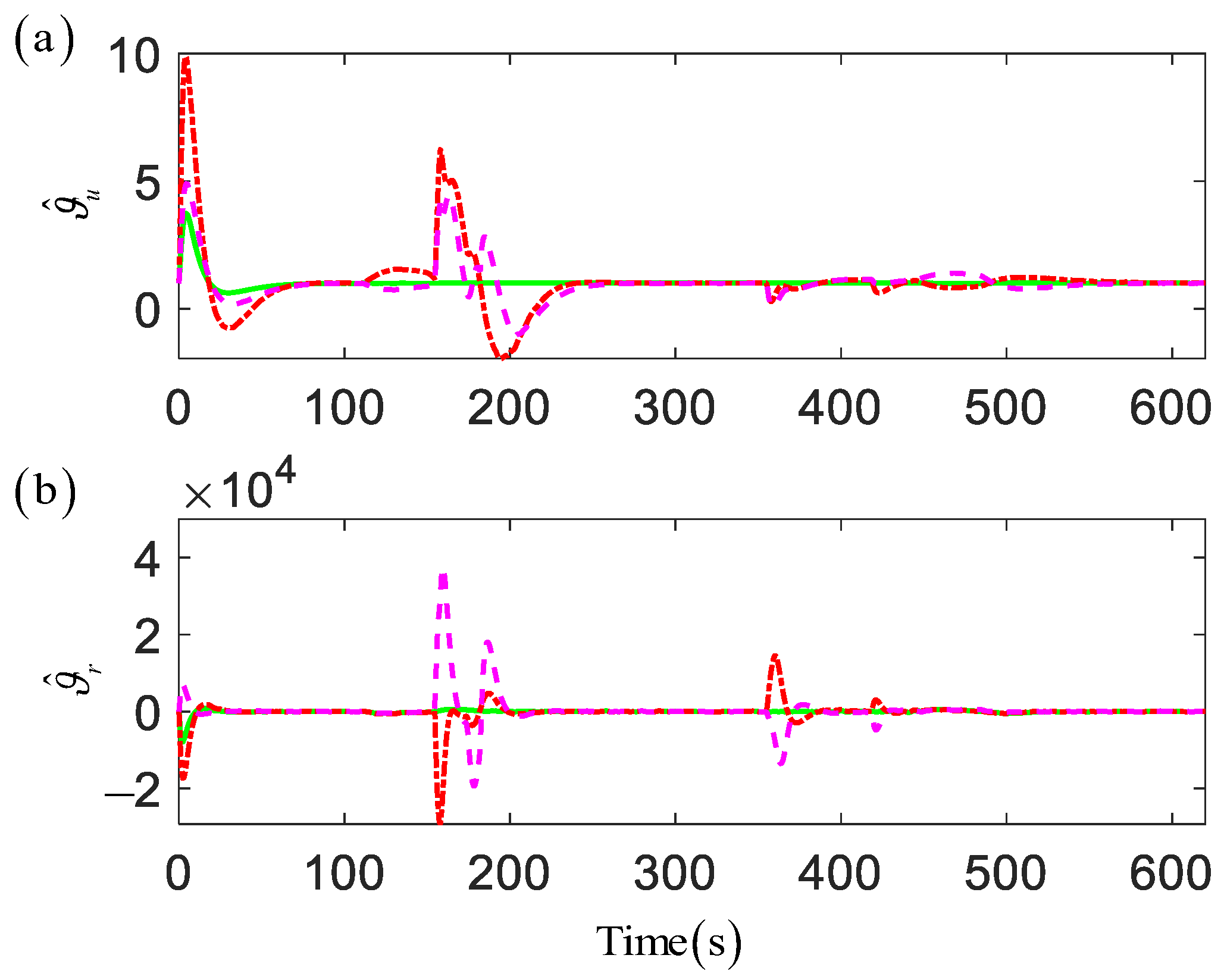
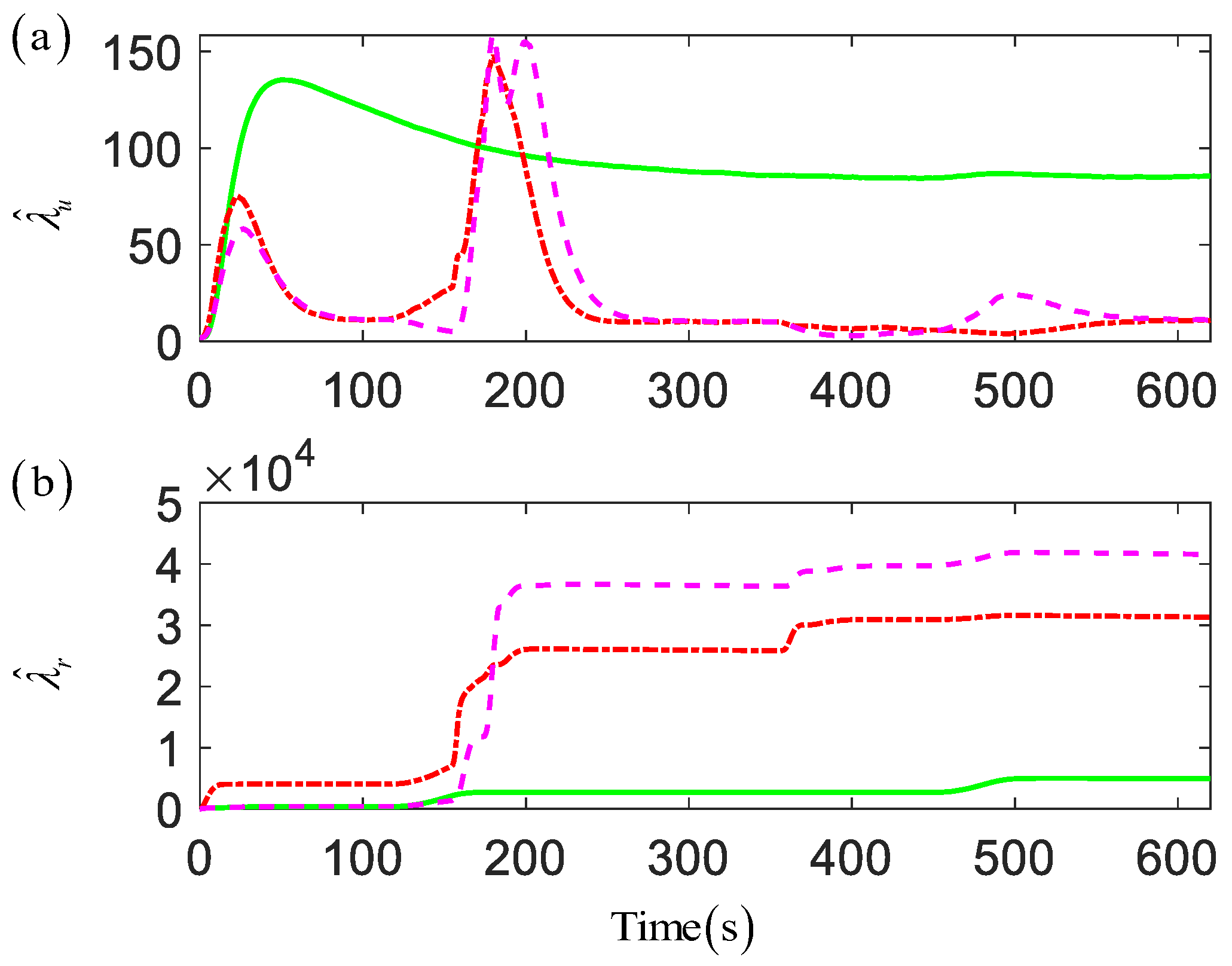
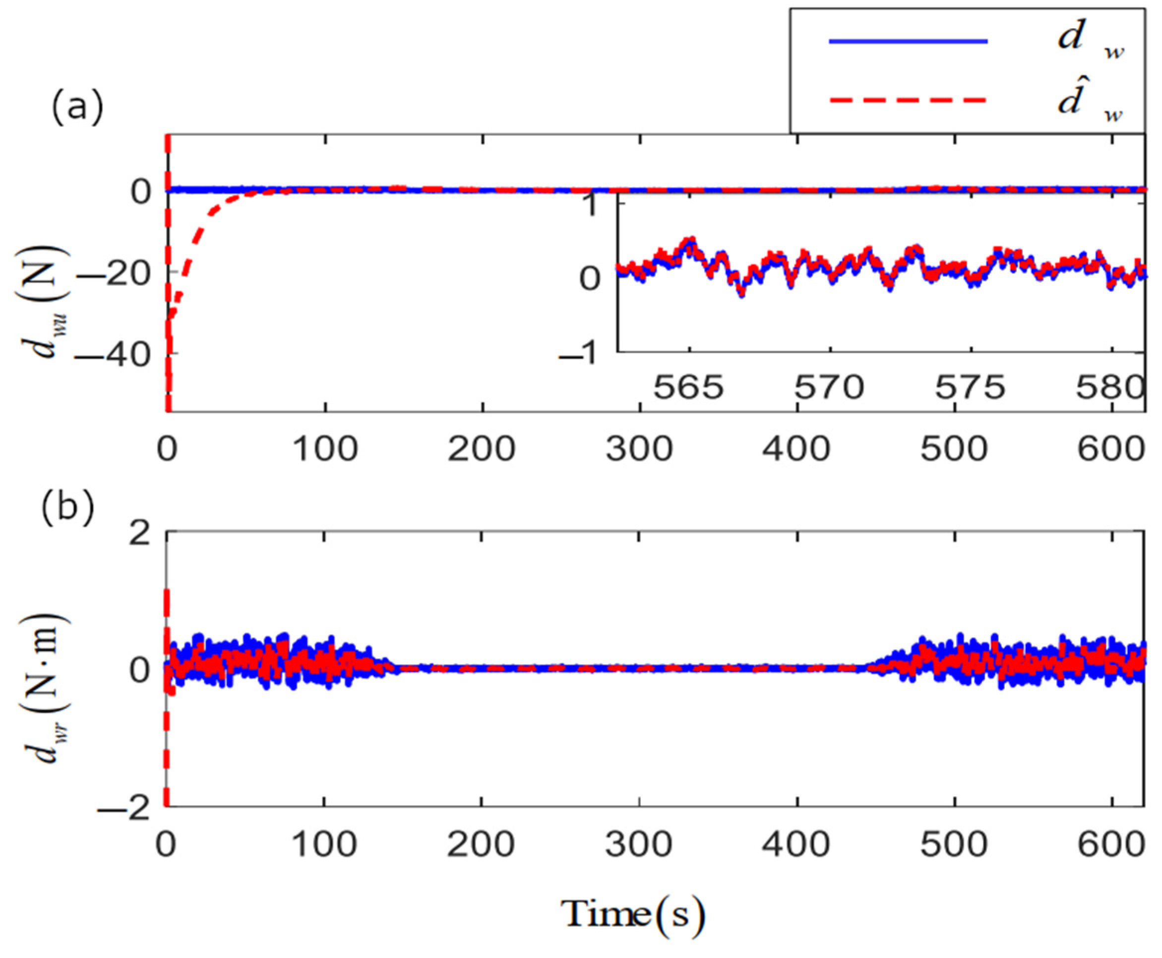
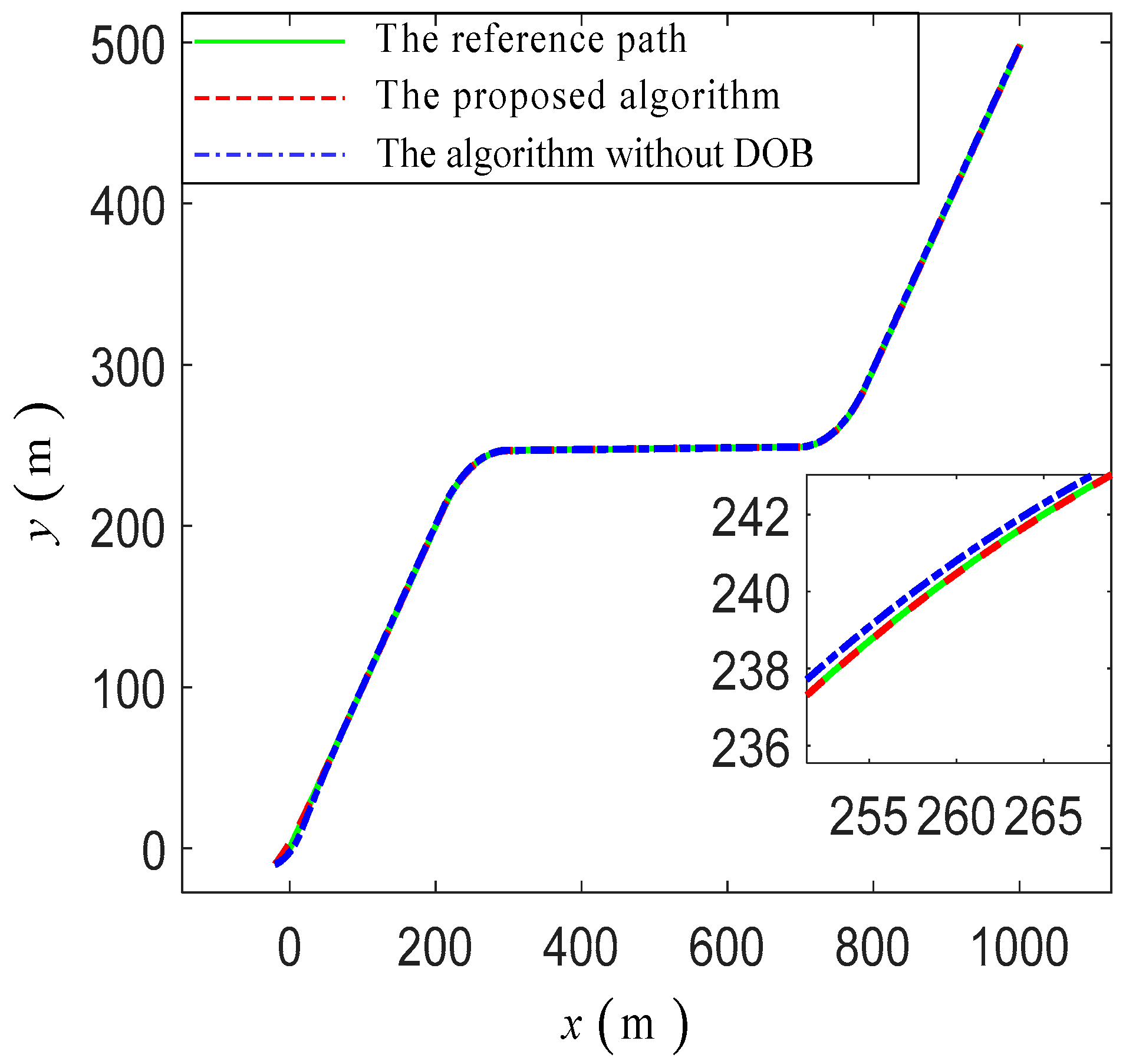
5. Numerical Experiment

In this section, two numerical simulative experiments are conducted to illustrate the superiority and effectiveness of the proposed guidance principle and control algorithm. Hence, the underactuated ship used in [18] with the length of $38\mathrm{m}$ and the mass of $118\times {10}^3\mathrm{kg}$ is chosen as the experimental subject.

5.1. Experiment under Restricted Water Area and Marine Environment

A waypoints-based path-following experiment was performed in fields of the narrow waterway and simulated marine environment. For this purpose, the reference path was generated by setting four waypoints: $W_1$$\left(700\mathrm{m},-500\mathrm{m}\right)$,$W_2$$\left(700\mathrm{m},550\mathrm{m}\right)$,$W_3$$\left(2500\mathrm{m},2550\mathrm{m}\right)$ and $W_4$$\left(2500\mathrm{m},3800\mathrm{m}\right)$. To navigate through the narrow waterway, the formation in the abreast structure needs to switch to a single file structure before sailing into the narrow waterway and then switch back to an abreast structure after sailing from the narrow waterway. For the guidance part, this process involves switching the bearing angles and distances between the GVS-leader and GVS-followers. The initial states of the USVs are expressed as $\left[x_1\left(0\right)\right.$,$y_1\left(0\right)$,${\psi }_1\left(0\right)$,$u_1\left(0\right)$,$v_1\left(0\right)$$\left.r_1\left(0\right)\right]$$=$$\left[670\mathrm{m}\right.$,$-700\mathrm{m}$,$\pi /4\mathrm{rad}$,$0\mathrm{m}/\mathrm{s}$,$0\mathrm{m}/\mathrm{s}$,$\left.0\mathrm{rad}/\mathrm{s}\right]$,$\left[x_2\left(0\right)\right.$,$y_2\left(0\right)$,${\psi }_2\left(0\right)$,$u_2\left(0\right)$,$v_2\left(0\right)$$\left.r_2\left(0\right)\right]$$=$$\left[520\mathrm{m}\right.$,$-700\mathrm{m}$,$\pi /4\mathrm{rad}$,$0\mathrm{m}/\mathrm{s}$,$0\mathrm{m}/\mathrm{s}$,$\left.0\mathrm{rad}/\mathrm{s}\right]$,$\left[x_3\left(0\right)\right.$,$y_3\left(0\right)$,${\psi }_3\left(0\right)$,$u_3\left(0\right)$,$v_3\left(0\right)$$\left.r_3\left(0\right)\right]$$=$$\left[880\mathrm{m}\right.$,$-700\mathrm{m}$,$\pi /4\mathrm{rad}$,$0\mathrm{m}/\mathrm{s}$,$0\mathrm{m}/\mathrm{s}$,$\left.0\mathrm{rad}/\mathrm{s}\right]$. The surge speed of the GVS-leader was chosen as $u_d=8\mathrm{m}/\mathrm{s}$, $u_m=5\mathrm{m}/\mathrm{s}$, and the configuration vectors for the GVS-followers were set as ${\iota }_1$$=\left[150\cos \left(\pi /2\right)\right.\mathrm{m}$,$150\sin \left(\pi /2\right)\mathrm{m}$,${\left.0\mathrm{rad}\right]}^{\mathrm{T}}$,${\iota }_2$$=\left[150\cos \left(-\pi /2\right)\right.\mathrm{m}$,$150\sin \left(-\pi /2\right)\mathrm{m}$,${\left.0\mathrm{rad}\right]}^{\mathrm{T}}$. After considering the ship length and the formation structure, ${\rho }_0=60\mathrm{m}$ was selected as the radius of the safety zones. The USVs were ordered to switch the formation structure before crossing the narrow channel and to reshape the structure once they were through the channel.

In the simulation, to verify the robustness of the proposed control algorithm, the external disturbances in nautical practice (sea wind and irregular wind-generated waves) were considered. The physical-based mathematical model based on the NORSOK (Norwegian Standards Organization) wind spectrum and the JONSWAP (Joint North Sea Wave Observation Project) wave spectrum was employed for a marine disturbance simulation [26]. Specifically, the main wind speed $U_{tw}=12.25\mathrm{m}/\mathrm{s}$ and the main wind direction ${\psi }_{tw}=3/8\mathrm{rad}$. The JONSWAP wave spectra were introduced to generate the time-varying wind-generated waves spectra with a sixth level sea state. The 2D sketch of the wind and 3D view of the waves are shown in Figure 4.

Figure 5, Figure 6, Figure 7, Figure 8, Figure 9, Figure 10, Figure 11 and Figure 12 describe the main numerical results of the proposed algorithm under the marine environment. Figure 5 describes the planar formation switch trajectories using the proposed scheme under the narrow waterway. Tracking errors of the position and direction can be seen in Figure 6. Obviously, the tracking errors were small enough compared with the scale of the formation route. Figure 7 describes the velocities of each USV. It shows that all the USVs reached the expected surge velocities in the formation-keeping period. While in the formation switch process, USV No. 2 and 3 regulated their surge velocities in order to adapt to the new formation structure. Additionally, for the purpose of sailing on the planned route with expected attitudes, the USVs’ sway and yaw velocities varied rapidly against the disturbances of the wind and waves. Figure 8 shows the control inputs ${\tau }_u$, ${\tau }_r$ of the USVs. Figure 9 and Figure 10 give the adaptive learning parameters ${\vartheta }_u$, ${\vartheta }_r$, ${\lambda }_u$, ${\lambda }_r$.

Figure 11 shows the distances between different USVs and if the USVs were at collision risks. In the proposed model, the collision avoidance is activated once the distances between two different USVs is less than $2{\rho }_0$. Additionally, it is assumed that the USVs are at high risks of collision when the distance is less than ${\rho }_0$. It is clear that all the USVs performed intervehicle collision avoidance well, and no USV was at a high risk of a collision. To clear the effectivity of the NNs-based disturbance observer, the marine disturbances $d_{wu}$, $d_{wr}$ and their estimations ${\widehat{d}}_{wu}$, ${\widehat{d}}_{wr}$ are exhibited in Figure 12. For clarity, we only illustrate the results of USV No. 1 in the following figures. Apparently, the USVs approximately followed the main wind direction of $W_2{W}_3$, so the disturbance in the sway moment of the force was smaller. This indicated that the simulated marine environment and NNs-based disturbance observer were effective.

5.2. Comparative Experiment

In this subsection, the proposed adaptive neural formation control algorithm is compared with the results of [15] in order to verify the superiority in terms of energy efficiency, robustness and control accuracy. Two underactuated ships consistent with the previous experiment are introduced in the comparative experiment. The curve path is generated by the desired yaw velocities as per Equation (61) and the desired surge velocities $u_d=10\left[1-0.8\exp \left(-2t\right)\right]\mathrm{m}/\mathrm{s}$. The initial states of the two underactuated ships are set as $\left[x\left(0\right),y\left(0\right),\psi \left(0\right),u\left(0\right),v\left(0\right),r\left(0\right)\right]=\left[-20\mathrm{m},-10\mathrm{m},\mathsf{\pi }/4\mathrm{rad},0\mathrm{m}/\mathrm{s},0\mathrm{m}/\mathrm{s},0\mathrm{rad}/\mathrm{s}\right]$:

$$r_d=\left\{\begin{array}{l}0\mathrm{rad}/\mathrm{s},t\in \left[0,30\right],\left(40,80\right],\left(90,120\right]\\ -0.078\mathrm{rad}/\mathrm{s},t\in \left(30,40\right]\\ 0.078\mathrm{rad}/\mathrm{s},t\in \left(80,90\right]\end{array}\right.$$

(61)

Therefore, the main comparative results are shown in Figure 13, Figure 14 and Figure 15. Figure 13 shows the path-following trajectories under two control algorithms. Both of the control algorithms performed reference path tracking with a satisfactory tracking accuracy. Still, the proposed control algorithm had a higher tracking accuracy. The comparison of the position and orientation errors under the two algorithms are displayed in Figure 14. Moreover, Figure 15 presents the control inputs under the two algorithms.

For further quantitative analysis, three useful performance indexes are introduced to evaluate the two algorithms as per Equation (62). The mean absolute error (MAE), the mean absolute control inputs (MAI) and the mean total inputs variation (MTV) describe the stabilization ability of the system, the energy consumption and the smoothness properties of the controllers, respectively. Detailed quantitative results are illustrated in

Table 1. Quantitative results for the proposed scheme and the one in [15].

Indexes	Items	The Proposed Algorithm	The Algorithm in [15]
MAE	$x_e\left(\mathrm{m}\right)$	$0.9742$	$1.5472$
	$y_e\left(\mathrm{m}\right)$	$0.0142$	$0.0593$
	${\psi }_e\left(\mathrm{deg}\right)$	$0.0153$	$0.0042$
MAI	${\tau }_u\left(\mathrm{N}\right)$	$2.9455\times {10}^6$	$2.9952\times {10}^6$
	${\tau }_r\left(\mathrm{N}\cdot \mathrm{m}\right)$	$7.6075\times {10}^6$	$1.2304\times {10}^7$
MTV	${\tau }_u\left(\mathrm{N}\right)$	$135.4431$	$7709.2$
	${\tau }_r\left(\mathrm{N}\cdot \mathrm{m}\right)$	$2.2678\times {10}^5$	$8.5352\times {10}^5$

. From the results, though the value of item ${\psi }_e$ in the proposed algorithm was larger than the value in [15], the values of the proposed algorithm were smaller than the related values in [15] on the whole. Therefore, the proposed algorithm has the superior advantages of a higher tracking accuracy, lower energy consumption and smoother energy variation:

$$\begin{array}{l}\mathrm{MAE}=\frac{1}{t_{end}-0}{\displaystyle {\int }_0^{t_{end}}\left|e\left(t\right)\right|dt}\\ \mathrm{MAI}=\frac{1}{t_{end}-0}{\displaystyle {\int }_0^{t_{end}}\left|\tau \left(t\right)\right|dt}\\ \mathrm{MTV}=\frac{1}{t_{end}-0}{\displaystyle {\int }_0^{t_{end}}\left|\tau \left(t+1\right)-\tau \left(t\right)\right|dt}\end{array}$$

(62)

6. Conclusions

This paper proposed a formation structure switch strategy for USVs while considering intervehicle collision avoidance. Unlike existing formation switch research that focuses on topology, the proposed guidance principle fully exploits the advantages of the leader–follower formation structure. By employing APSs, flexible and safe paths are planned for USVs without using the unknown velocity information of the GVS-followers. The DOB-based robust neural formation control algorithm performed formation tracking excellently. Moreover, profiting from the NNs-based disturbance observer, the unmeasurable marine disturbances can be estimated accurately, which can lower the actual inputs and energy consumption.

In future work, we will focus on gradually changing the vehicle’s velocity while performing a formation switch task.

References

1. Cui, R.; Ge, S.S.; How, B.V.E.; Choo, Y.S. Leader-follower formation control of underactuated AUVs with leader position measurement. In Proceedings of the IEEE International Conference on Robotics and Automation, Kobe, Japan, 12–17 May 2009; pp. 979–984. [Google Scholar]
2. Ren, W.; Beard, R.; Atkins, E. A survey of consensus problems in multi-agent coordination. In Proceedings of the American Control Conference, Portland, OR, USA, 8–10 June 2005; pp. 1859–1864. [Google Scholar]
3. Ren, W.; Beard, R.W. Formation feedback control for multiple spacecraft via virtual structures. Control. Theory Appl. 2004, 151, 357–368. [Google Scholar]
4. Balch, T.; Arkin, R. Behavior-based formation control for multirobot teams. IEEE Trans. Robot. Autom. 1998, 14, 926–939. [Google Scholar]
5. Zhang, G.; Liu, S.; Zhang, X.; Zhang, W. Event-Triggered Cooperative Formation Control for Autonomous Surface Vehicles Under the Maritime Search Operation. IEEE Trans. Intell. Transp. Syst. 2022, 23, 21392–21404. [Google Scholar]
6. Liu, L.; Wang, D.; Peng, Z.; Li, T.; Chen, C.L.P. Cooperative Path Following Ring-Networked Under-Actuated Autonomous Surface Vehicles: Algorithms and Experimental Results. IEEE Trans. Cybern. 2020, 50, 1519–1529. [Google Scholar]
7. Wang, Y.; Liu, Y.; Li, X.; Liang, Y. Distributed consensus tracking control based on state and disturbance observations for mixed-order multiagent mechanical systems. J. Frankl. Inst. 2023, 360, 943–963. [Google Scholar]
8. Liu, C.; Hu, Q.; Sun, T. Distributed formation control of underactuated ships with connectivity preservation and collision avoidance. Ocean. Eng. 2022, 263, 112350. [Google Scholar]
9. Du, X.; Li, W.; Xiao, J.; Chen, Z. Time-Varying Group Formation with Adaptive Control for Second-Order Multi-Agent Systems. IEEE Access 2022, 10, 45337–45346. [Google Scholar]
10. Zhang, G.; Huang, C.; Li, J.; Zhang, X. Constrained coordinated path-following control for underactuated surface vessels with the disturbance rejection mechanism. Ocean. Eng. 2020, 196, 106725. [Google Scholar]
11. Liang, X.; Qu, X.; Wang, N.; Li, Y.; Zhang, R. Swarm control with collision avoidance for multiple underactuated surface vehicles. Ocean. Eng. 2019, 191, 106516. [Google Scholar]
12. Chen, L.; Hopman, H.; Negenborn, R.R. Distributed Model Predictive Control for cooperative floating object transport with multi-vessel systems. Ocean. Eng. 2019, 191, 106515. [Google Scholar]
13. Shojaei, K. Observer-based neural adaptive formation control of autonomous surface vessels with limited torque. Robot. Auton. Syst. 2016, 78, 83–96. [Google Scholar]
14. Huang, C.; Zhang, X.; Zhang, G. Adaptive neural finite-time formation control for multiple underactuated vessels with actuator faults. Ocean. Eng. 2021, 222, 108556. [Google Scholar]
15. Zhang, G.; Liu, S.; Li, J.; Zhang, X. LVS guidance principle and adaptive neural fault-tolerant formation control for underactuated vehicles with the event-triggered input. Ocean. Eng. 2021, 229, 108927. [Google Scholar]
16. Khatib, O. Real-time obstacle avoidance for manipulators and mobile robots. In Proceedings of the IEEE International Conference on Robotics and Automation, St. Louis, MO, USA, 25–28 March 1985; Volume 2, pp. 500–505. [Google Scholar]
17. Zhang, G.; Han, J.; Li, J.; Zhang, X. APF-based intelligent navigation approach for USV in presence of mixed potential directions: Guidance and control design. Ocean. Eng. 2022, 260, 111972. [Google Scholar]
18. Zhang, G.; Zhang, X. Concise Robust Adaptive Path-Following Control of Underactuated Ships Using DSC and MLP. IEEE J. Ocean. Eng. 2014, 39, 685–694. [Google Scholar]
19. Zhang, G.; Li, J.; Jin, X.; Liu, C. Robust Adaptive Neural Control for Wing-Sail-Assisted Vehicle via the Multiport Event-Triggered Approach. IEEE Trans. Cybern. 2022, 52, 12916–12928. [Google Scholar]
20. Li, J.; Zhang, G.; Shan, Q.; Zhang, W. A Novel Cooperative Design for USV-UAV Systems: 3D Mapping Guidance and Adaptive Fuzzy Control. IEEE Trans. Control. Netw. Syst. 2022, in press. [Google Scholar] [CrossRef]
21. Zhang, G.; Zhang, C.; Lang, L.; Zhang, W. Practical constrained output feedback formation control of underactuated vehicles via the autonomous dynamic logic guidance. J. Frankl. Inst. 2021, 358, 6566–6591. [Google Scholar]
22. Lin, F.; Zhang, J.; Jia, X.; Zhou, X. Adaptive event-triggering distributed filter of positive markovian jump systems based on disturbance observer. J. Frankl. Inst. 2023, 360, 2507–2537. [Google Scholar]
23. Do, K. Practical control of underactuated ships. Ocean. Eng. 2010, 37, 1111–1119. [Google Scholar]
24. Du, J.; Hu, X.; Krstic, M.; Sun, Y. Robust dynamic positioning of ships with disturbances under input saturation. Automatica 2016, 73, 207–214. [Google Scholar]
25. Lu, Y.; Zhang, G.; Sun, Z.; Zhang, W. Robust adaptive formation control of underactuated autonomous surface vessels based on MLP and DOB. Nonlinear Dyn. 2018, 94, 503–519. [Google Scholar]
26. Fossen, T.I. Handbook of Marine Craft Hydrodynamics and Motion Control; John Wiley & Sons: Hoboken, NJ, USA, 2011. [Google Scholar]
27. Li, J.H.; Lee, P.M.; Jun, B.H.; Lim, Y.K. Point-to-point navigation of underactuated ships. Automatica 2008, 44, 3201–3205. [Google Scholar]
28. Ren, B.; San, P.P.; Ge, S.S.; Lee, T.H. Adaptive dynamic surface control for a class of strict-feedback nonlinear systems with unknown backlash-like hysteresis. In Proceedings of the American Control Conference, St. Louis, MO, USA, 10–12 June 2009; pp. 4482–4487. [Google Scholar]
29. Li, Y.; Tong, S. Adaptive neural networks prescribed performance control design for switched interconnected uncertain non-linear systems. IEEE Trans. Neural Netw. Learn. Syst. 2017, 29, 3059–3068. [Google Scholar]
30. Zhang, G.; Zhang, X. A novel DVS guidance principle and robust adaptive path-following control for underactuated ships using low frequency gain-learning. ISA Trans. 2015, 56, 75–85. [Google Scholar]
31. Li, T.S.; Wang, D.; Feng, G.; Tong, S.C. A DSC Approach to Robust Adaptive NN Tracking Control for Strict-Feedback Nonlinear Systems. IEEE Trans. Syst. Man Cybern. Part B 2010, 40, 915–927. [Google Scholar]
32. Zhang, X.; Jia, X.; Wang, X. A kind of transfigured loop shaping controller and its application. Autom. Control. Comput. Sci. 2001, 35, 20–25. [Google Scholar]
Figure 1. The framework of APS-based leader–follower formation structure.
Jmse 11 01020 g001
Figure 2. The processes and details of formation switch.
Jmse 11 01020 g002
Figure 3. The block diagram of the proposed robust adaptative formation control scheme.
Jmse 11 01020 g003
Figure 4. The simulated marine environment: (a) 2D sketch field of surface wind; (b) 3D view of the wind-generated waves.
Jmse 11 01020 g004
Figure 5. The formation switch performance under the narrow waterway and simulated ocean environment.
Jmse 11 01020 g005
Figure 6. Tracking errors of USVs in position and orientation: (a,b) error curves of position; (c) error curves of orientation.
Jmse 11 01020 g006
Figure 7. Velocities of USVs: (a) surge velocities; (b) sway velocities; (c) yaw velocities.
Jmse 11 01020 g007
Figure 8. Control inputs of USVs: (a) control inputs of the propeller; (b) control inputs of the rudder.
Jmse 11 01020 g008
Figure 9. Adaptive parameters ϑ ^ u and ϑ ^ r of USVs: (a) adaptive parameters for surge motion; (b) adaptive parameters for yaw motion.
Jmse 11 01020 g009
Figure 10. Adaptive parameters λ ^ u and λ ^ r of USVs: (a) adaptive parameters for surge motion; (b) adaptive parameters for yaw motion.
Jmse 11 01020 g010
Figure 11. The distances between different USVs.
Jmse 11 01020 g011
Figure 12. The performance of NNs-based DOB: (a) marine disturbances d w u and its estimation d ^ w u ; (b) marine disturbances d w r and its estimation d ^ w r .
Jmse 11 01020 g012
Figure 13. The tracking path under different control algorithms.
Jmse 11 01020 g013
Figure 14. The tracking errors of two control algorithms: (a,b) error curves of position; (c) error curves of orientation.
Jmse 11 01020 g014
Figure 15. Control inputs of two control algorithms: (a) control inputs of the propeller; (b) control inputs of the rudder.
Jmse 11 01020 g015