


A Comparative Study to Estimate Fuel Consumption: A Simplified Physical Approach against a Data-Driven Model

 ,
,  ,
,  ,
,  and
and
Abstract
1. Introduction
1.1. The Problem of Reducing Ship Fuel Consumption
1.2. Studies on Ship Fuel Consumption
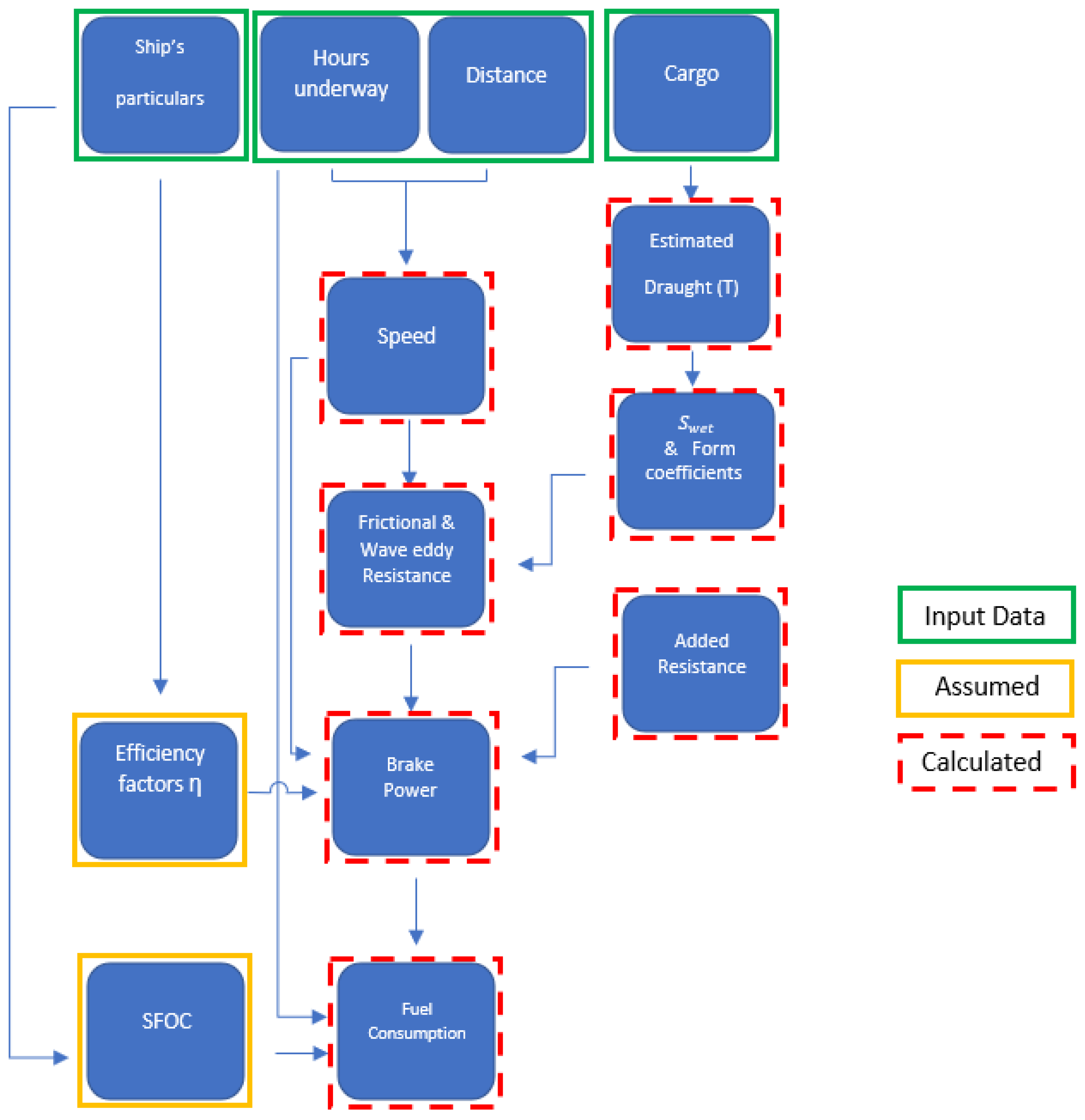
2. The SNAM
- (1)
- Determination of calm water resistance via the ship’s approximate draft and the available information regarding the cargo being transported.
- (2)
- Determination of the approximated added resistance caused by waves and wind.
- (3)
- Approximation of the efficiency factors representing the overall propulsion chain.
- (4)
- Determination of the brake power via the total resistance obtained from step 1, the efficiency factor obtained from step 3, and the ship’s voyage speed.
- (5)
- Estimation of fuel consumption via the product of the hours underway, the brake power obtained from step 4, and the approximated specific fuel oil consumption (SFOC) based on the ship’s principal particulars.
- RF is the frictional resistance;
- k1 is the form factor describing the viscous resistance of the hull;
- RAPP is the appendage resistance;
- Rw is the added resistance in waves;
- RB is the additional pressure resistance of a bulbous bow;
- RTR is the additional pressure resistance of an immersed transom;
- RA is the model ship correlation resistance;
- Rwind is the wind resistance.
- B is the beam of the ship;
- ρ is the water density;
- is the significant wave height;
- is the length of the bow on the waterline at 95% of B.
- Hours underway;
- Cargo weight transported;
- Total voyage distance.
- Lbp is the length between perpendiculars;
- CM is the midship section coefficient for the sampled voyage;
- CB is the block coefficient for the sampled voyage;
- CWP is the water plane area coefficient for the sampled voyage;
- TDD is the draft for the sampled voyage;
- ABT is the transverse sectional area of the bulb at the position where the calm water surface intersects the stem.
2.1. Draft Determination
- DP is the assumed propeller diameter, approximated as 0.65 of design draft;
- e is the distance of lower extremity of the propeller blades to the base;
- L is the ship’s length.
- C = 0.4;
- CBD is the block coefficient at design draft;
- TD is the design draft.
- ∆ is the approximated displacement during the voyage;
- CWD is the water plane area coefficient at design draft;
- ∆O is the approximated displacement of design draft.
2.2. Brake Power
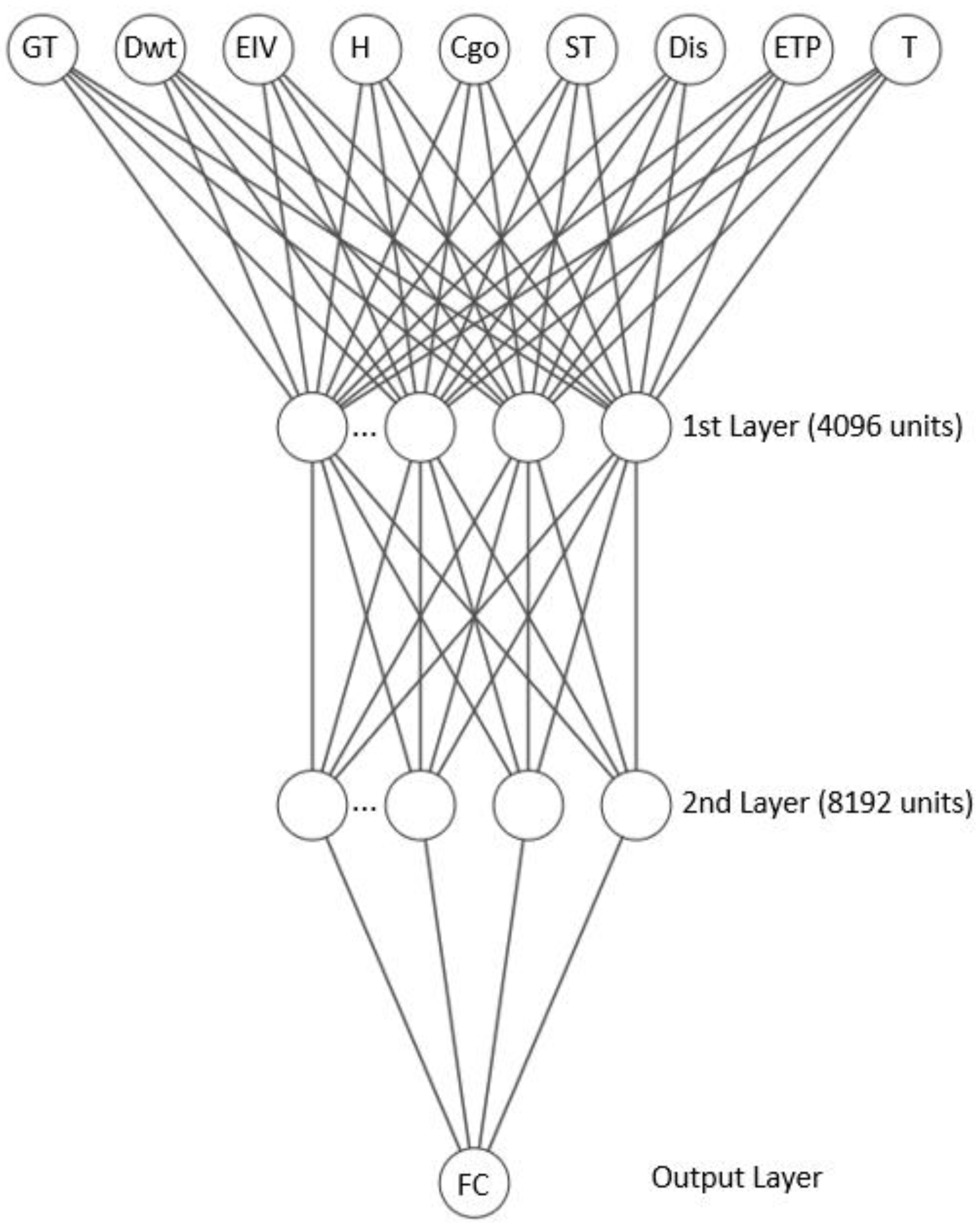
3. The DNN Approach
- Gross tonnage (GT);
- Maximum deadweight (Dwt);
- Efficiency value (EIV);
- Hours underway (H);
- Cargo transported (Cgo);
- Ship type (ST);
- Distance (Dis);
- Engine total output power (ETP);
- Draft (T).
4. Results and Discussion
5. Conclusions
Author Contributions
Funding
Institutional Review Board Statement
Informed Consent Statement
Data Availability Statement
Conflicts of Interest
References
- IMO. RESOLUTION MEPC.353(78). 2022. Available online: https://wwwcdn.imo.org/localresources/en/OurWork/Environment/Documents/Air%20pollution/MEPC.353(78).pdf (accessed on 28 March 2023).
- Padhy, C.P.; Sen, D.; Bhaskaran, P.K. Application of wave model for weather routing of ships in the North Indian Ocean. Nat. Hazards 2007, 44, 373–385. [Google Scholar] [CrossRef]
- Armstrong, N. Review—Ship optimisation for low carbon shipping. Ocean. Eng. 2013, 73, 195–207. [Google Scholar] [CrossRef]
- Mezaoui, B.; Takashima, K.; Shoji, R. On the fuel saving operation for coastal merchant ships using weather routing. In Marine Navigation and Safety of Sea Transportation; CRC Press: Boca Raton, FL, USA, 2009; Volume 6. [Google Scholar]
- Adland, R.; Cariou, P.; Wolff, F.-C. Optimal ship speed and the cubic law revisited: Empirical evidence from an oil tanker fleet. Transp. Res. Part E Logist. Transp. Rev. 2020, 140, 101972. [Google Scholar] [CrossRef]
- IMO. MEPC 76/15/Add.2. 2021. Available online: https://wwwcdn.imo.org/localresources/en/OurWork/Environment/Documents/Air%20pollution/MEPC.333(76).pdf (accessed on 28 March 2023).
- Kim, J.-G.; Kim, H.-J.; Jun, H.B.; Kim, C.-M. Optimizing Ship Speed to Minimize Total Fuel Consumption with Multiple Time Windows. Math. Probl. Eng. 2016, 2016, 3130291. [Google Scholar] [CrossRef]
- Ronen, D. Effect of oil price on the optimal speed of ships. J. Oper. Res. Soc. 1982, 33, 1035–1040. [Google Scholar] [CrossRef]
- Adland, R.; Cariou, P.; Jia, H.; Wolff, F. The energy efficiency effects of periodic ship hull cleaning. J. Clean. Prod. 2018, 178, 1–13. [Google Scholar] [CrossRef]
- Wilkinson, C.-P. Reductions in fuel consumption as a result of in-water propeller polishing. In Proceeding of the Propellers ’88 Symposium, Virginia Beach, VA, USA, 20–21 September 1988. [Google Scholar]
- Braidotti, L.; Mauro, F.; Sebastiani, L.; Bisiani, S.; Bucci, V. A Ballast Allocation Technique to Minimize Fuel Consumption. In Proceedings of the 19th International Conference on Ships and Maritime Research—NAV 2018, Trieste, Italy, 20–22 June 2018. [Google Scholar]
- Mewis, F.; Guiard, T. Mewis Duct®—New Developments, Solutions and Conclusions. In Proceedings of the Second International Symposium on Marine Propulsors, Hamburg, Germany, 15–17 June 2011. [Google Scholar]
- Fan, A.; Yang, J.; Yang, L.; Wu, D.; Vladimir, N. A review of ship fuel consumption models. Ocean Eng. 2022, 264, 112405. [Google Scholar] [CrossRef]
- Kim, K.S.; Roh, M.I. ISO 15016:2015-Based Method for Estimating the Fuel Oil Consumption of a Ship. J. Mar. Sci. Eng. 2020, 8, 791. [Google Scholar] [CrossRef]
- Bialystocki, N.; Konovessis, D. On the estimation of ship’s fuel consumption and speed curve: A statistical approach. J. Ocean Eng. Sci. 2016, 1, 157–166. [Google Scholar] [CrossRef]
- Wang, S.; Ji, B.; Zhao, J.; Liu, W.; Xu, T. Predicting ship fuel consumption based on LASSO regression. Transp. Res. Part D Transp. Environ. 2018, 65, 817–824. [Google Scholar] [CrossRef]
- Bocchetti, D.; Lepore, A.; Palumbo, B.; Vitiello, L. A statistical approach to ship fuel consumption monitoring. J. Ship Res. 2015, 59, 162–171. [Google Scholar] [CrossRef]
- Jeon, M.; Noh, Y.; Shin, Y.; Lim, O.-K.; Lee, I.; Cho, D. Prediction of ship fuel consumption by using an artificial neural network. J. Mech. Sci. Technol. 2018, 32, 5785–5796. [Google Scholar] [CrossRef]
- Tarelko, W.; Rudzki, K. Applying artificial neural networks for modelling ship speed and fuel consumption. Neural Comput. Appl. 2020, 32, 17379–17395. [Google Scholar] [CrossRef]
- Petersen, J.P.; Jacobsen, D.J.; Winther, O. Statistical modelling for ship propulsion efficiency. J. Mar. Sci. Technol. 2012, 17, 30–39. [Google Scholar] [CrossRef]
- Le, L.T.; Lee, G.; Park, K.S.; Kim, H. Neural network-based fuel consumption estimation for container ships in Korea. Marit. Policy Manag. 2020, 47, 615–632. [Google Scholar] [CrossRef]
- Kim, Y.-R.; Jung, M.; Park, J.-B. Development of a Fuel Consumption Prediction Model Based on Machine Learning Using Ship In-Service Data. J. Mar. Sci. Eng. 2021, 9, 137. [Google Scholar] [CrossRef]
- Haranen, M.; Pakkanen, P.; Kariranta, R.; Salo, J. White, Grey and Black-Box Modelling in Ship Performance Evaluation. In Proceedings of the 1st Hull Performance & Insight Conference, Castello di Pavone, Italy, 13–15 April 2016. [Google Scholar]
- Esmailian, E.; Steen, S. A new method for optimal ship design in real sea states using the ship power profile. Ocean. Eng. 2022, 259, 111893. [Google Scholar] [CrossRef]
- Holtrop, J.; Mennen, G. An approximate power prediction method. Int. Shipbuild. Prog. 1982, 29, 166–170. [Google Scholar] [CrossRef]
- Guldhammer, H.E.; Harvald, S.A. Ship Resistance—Effect of Form and Principal Dimensions; Akademisk Forlag: Copenhagen, Denmark, 1974. [Google Scholar]
- Hollenbach, K. Estimating resistance and propulsion for single-screw and twin-screw ships. Ship Technol. Res. 1998, 45, 72–76. [Google Scholar]
- Pérez, A.F. Some methods to obtain the added resistance of a ship advancing in waves. Ocean. Eng. 2007, 34, 946–955. [Google Scholar] [CrossRef]
- ISO 15016; 2015-Ship and Marine Technology-Guidelines for the Assessment of Speed and Power Performance Analysis of Speed Trial Data. ISO: Geneva, Switzerland, 2015.
- MAN Energy Solution SE, Basic Principle of Ship Propulsion, Copenhagen SV, Denmark. 2018. Available online: https://www.man-es.com/docs/default-source/marine/tools/basic-principles-of-ship-propulsion_web_links.pdf?sfvrsn=12d1b862_10 (accessed on 28 March 2023).
- Papanikolaou, A. Ship Design—Methodologies of Preliminary Design; Springer: Berlin/Heidelberg, Germany, 2014; pp. 137, 244. [Google Scholar]
- Riesner, M.; El Moctar, O.; Schellin, T.E. Design Related Speed Loss and Fuel Consumption of Ships in Seaways. In Proceedings of the MARTECH 2018—4th International Conference on Maritime Technology and Engineering, Lisbon, Portugal, 7–9 May 2018. [Google Scholar]
- I.M.O. Second IMO Greenhouse Gas Study. 2009. Available online: https://www.imo.org/en/OurWork/Environment/Pages/Greenhouse-Gas-Study-2009.aspx (accessed on 28 March 2023).
- Prihandanu, R.B.; Ariana, I.M.; Handani, D.W. Analysis of Stern Shape Effect on Pre-Duct Propeller Performance Based on Numerical Simulation. IOP Conf. Ser. Mater. Sci. Eng. 2021, 1052, 012016. [Google Scholar] [CrossRef]
- Xing, H.; Spence, S.; Chen, H. A comprehensive review on countermeasures for CO2 emissions from ships. Renew. Sustain. Energy Rev. 2020, 134, 110222. [Google Scholar] [CrossRef]
- Saleem, R.; Yuan, B.; Kurugollu, F.; Anjum, A.; Liu, L. Explaining deep neural networks: A survey on the global interpretation methods. Neurocomputing 2022, 513, 165–180. [Google Scholar] [CrossRef]
- Haykin, S. Neural Networks: A Comprehensive Foundation; Pearson Prentice Hall: Hoboken, NJ, USA, 1994. [Google Scholar]
- Cybenko, G. Approximation by superpositions of a sigmoidal function. Math. Control. Signals Syst. 1989, 2, 303–314. [Google Scholar] [CrossRef]
- Ramachandran, P.; Zoph, B.; Le, Q.V. Searching for activation functions. arXiv 2017, arXiv:1710.05941. [Google Scholar]
- La Ferlita, A.; Di Nardo, E.; Macera, M.; Lindemann, T.; Ciaramella, A.; Kaeding, P. Deep Neural Network (DNN) Method to predict the displacement behavior of neutral axis for ships in vertical bending. In Proceedings of the 20th International Conference on Ship and Maritime Research (NAV2022), Genoa, Italy, 15–17 June 2022. [Google Scholar]
- Kingma, D.P.; Ba, J. Adam: A method for stochastic optimization. arXiv 2014, arXiv:1412.6980. [Google Scholar]
- Bengio, Y. Practical recommendations for gradient-based training of deep architectures. In Neural Networks: Tricks of the Trade; Springer: Berlin/Heidelberg, Germany, 2012; pp. 437–478. [Google Scholar]
- Girshick, R. Fast r-cnn. In Proceedings of the IEEE International Conference on Computer Vision, Santiago, Chile, 7–13 December 2015; pp. 1440–1448. [Google Scholar]
- La Ferlita, A.; Di Nardo, E.; Macera, M.; Lindemann, T.; Ciaramella, A.; Koulianos, N. A Deep Neural Network to Predict the Residual Hull Girder Strenght. In SNAME 2022; OnePetro: Houston, TX, USA, 2022. [Google Scholar]


| Engine Age | Power Output above 15,000 kW | Power Output between 15,000 and 5000 kW |
|---|---|---|
| Before 1983 | 205 | 215 |
| 1984–2000 | 185 | 195 |
| 2001–2007 | 175 | 185 |
| Efficiency Factor | Assumed Value | Literature |
|---|---|---|
| (relative rotative) | (single screw) 1.00–1.07 | [34] |
| (twin screw) 0.98 | [30] | |
| (hull) | 1.10–1.30 | [30] |
| (shaft) | 0.95–0.99 | [30] |
| (propeller—open water) | 0.55–0.70 | [35] |
| Ship Topology | Number of Ships | Number of Voyages |
|---|---|---|
| General cargo ship | 61 | 433 |
| Oil tanker | 52 | 324 |
| Containership | 300 | 10,805 |
| RoRo ship | 2 | 236 |
| Bulk carrier | 147 | 765 |
| Ship Topology | Number of Ships | Number of Voyages |
|---|---|---|
| General cargo ship | 14 | 100 |
| Oil tanker | 9 | 100 |
| Containership | 2 | 100 |
| RoRo ship | 4 | 100 |
| Bulk carrier | 9 | 70 |
| Ship Topology | Normalized RMSE (SNAM) | Normalized RMSE (DNN Method) | Loss Value |
|---|---|---|---|
| Bulk carrier | 0.062 | 0.032 | 0.0067059 |
| Oil tanker | 0.105 | 0.050 | 0.0373286 |
| Containership | 0.086 | 0.267 | 0.0590038 |
| General cargo ship | 0.062 | 0.082 | 0.0212367 |
| RoRo ship | 0.061 | 0.052 | 0.0060399 |
Disclaimer/Publisher’s Note: The statements, opinions and data contained in all publications are solely those of the individual author(s) and contributor(s) and not of MDPI and/or the editor(s). MDPI and/or the editor(s) disclaim responsibility for any injury to people or property resulting from any ideas, methods, instructions or products referred to in the content. |
© 2023 by the authors. Licensee MDPI, Basel, Switzerland. This article is an open access article distributed under the terms and conditions of the Creative Commons Attribution (CC BY) license (https://creativecommons.org/licenses/by/4.0/).
Share and Cite
La Ferlita, A.; Qi, Y.; Di Nardo, E.; el Moctar, O.; Schellin, T.E.; Ciaramella, A. A Comparative Study to Estimate Fuel Consumption: A Simplified Physical Approach against a Data-Driven Model. J. Mar. Sci. Eng. 2023, 11, 850. https://doi.org/10.3390/jmse11040850
La Ferlita A, Qi Y, Di Nardo E, el Moctar O, Schellin TE, Ciaramella A. A Comparative Study to Estimate Fuel Consumption: A Simplified Physical Approach against a Data-Driven Model. Journal of Marine Science and Engineering. 2023; 11(4):850. https://doi.org/10.3390/jmse11040850
Chicago/Turabian StyleLa Ferlita, Alessandro, Yan Qi, Emanuel Di Nardo, Ould el Moctar, Thomas E. Schellin, and Angelo Ciaramella. 2023. "A Comparative Study to Estimate Fuel Consumption: A Simplified Physical Approach against a Data-Driven Model" Journal of Marine Science and Engineering 11, no. 4: 850. https://doi.org/10.3390/jmse11040850
APA StyleLa Ferlita, A., Qi, Y., Di Nardo, E., el Moctar, O., Schellin, T. E., & Ciaramella, A. (2023). A Comparative Study to Estimate Fuel Consumption: A Simplified Physical Approach against a Data-Driven Model. Journal of Marine Science and Engineering, 11(4), 850. https://doi.org/10.3390/jmse11040850