
Path Planning of an Unmanned Surface Vessel Based on the Improved A-Star and Dynamic Window Method


Abstract
:1. Introduction
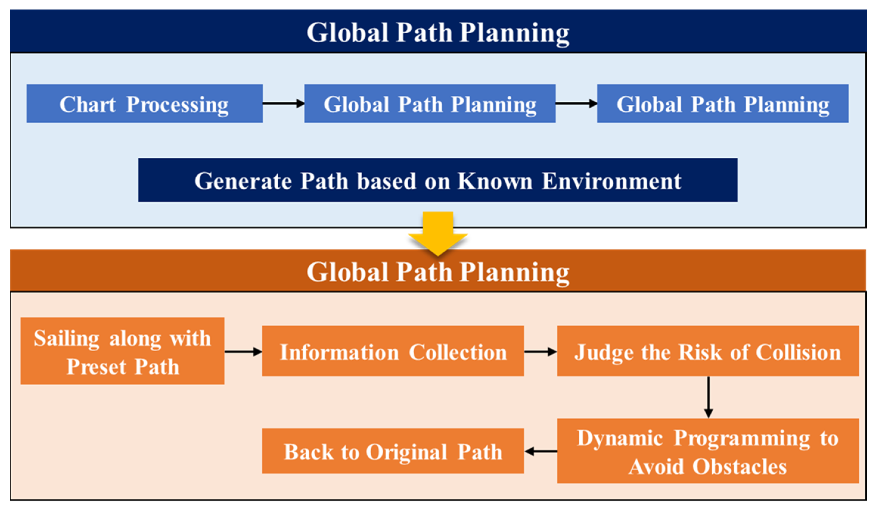
2. Global Path Planning of USV Based on an Electronic Navigation Chart
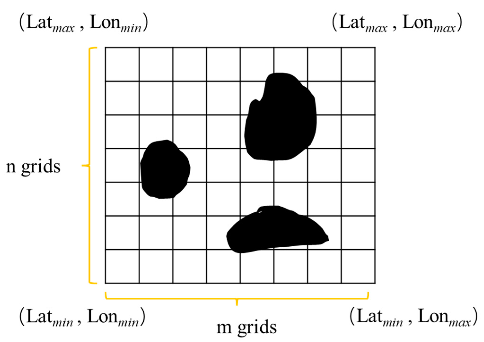
2.1. Chart Data Processing
2.2. Improved A-Star Algorithm
3. Local Path Planning of USV
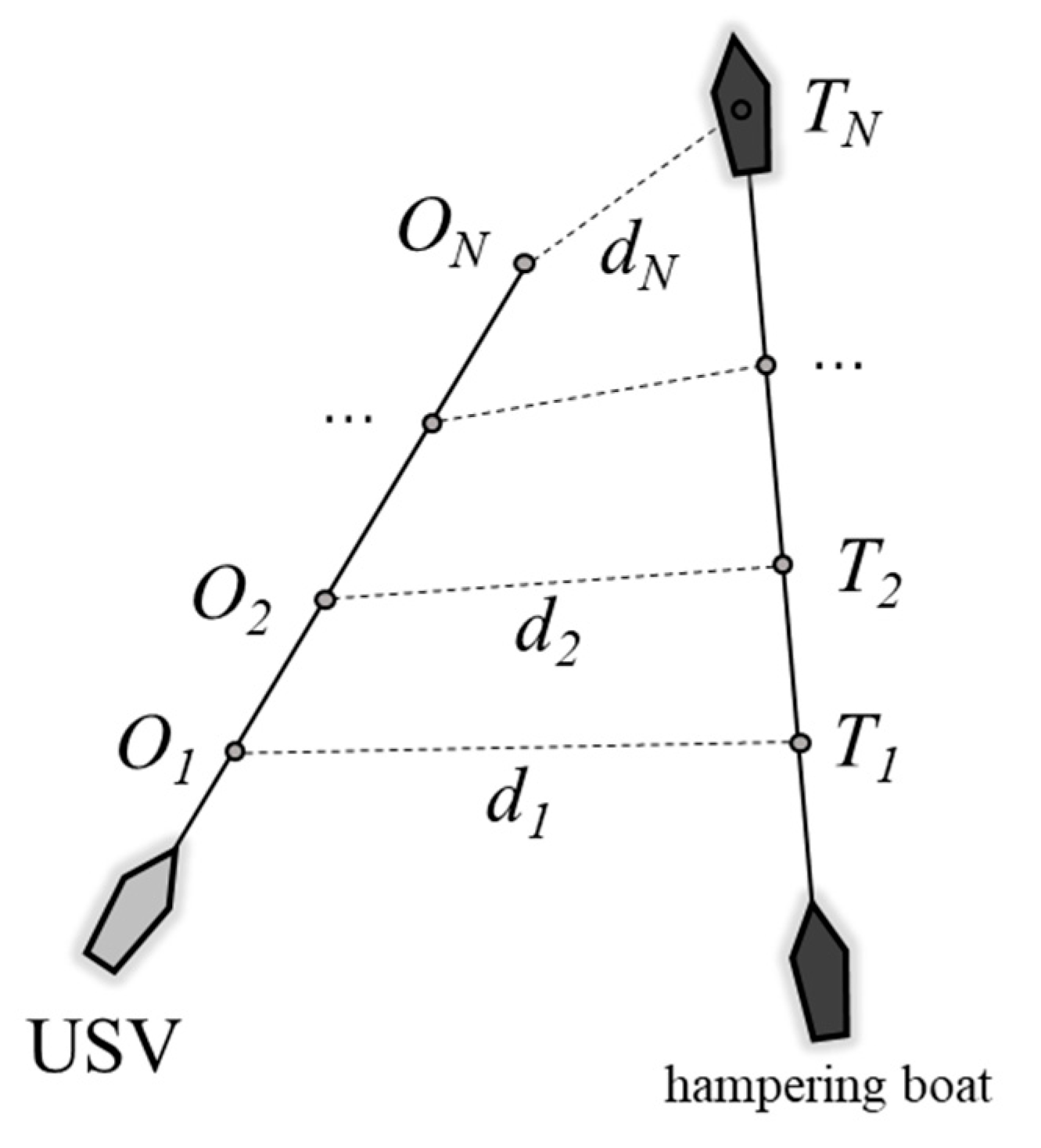
3.1. Collision Avoidance Decision Based on the Dynamic Window Method
- (1)
- Velocity constraints
- (2)
- Performance constraints of USV
- (3)
- Stopping distance constraint
3.2. Acquisition of Optimal Trajectory
- (1)
- Trajectory preprocessing
- (2)
- Trajectory evaluation function
4. Results and Discussion
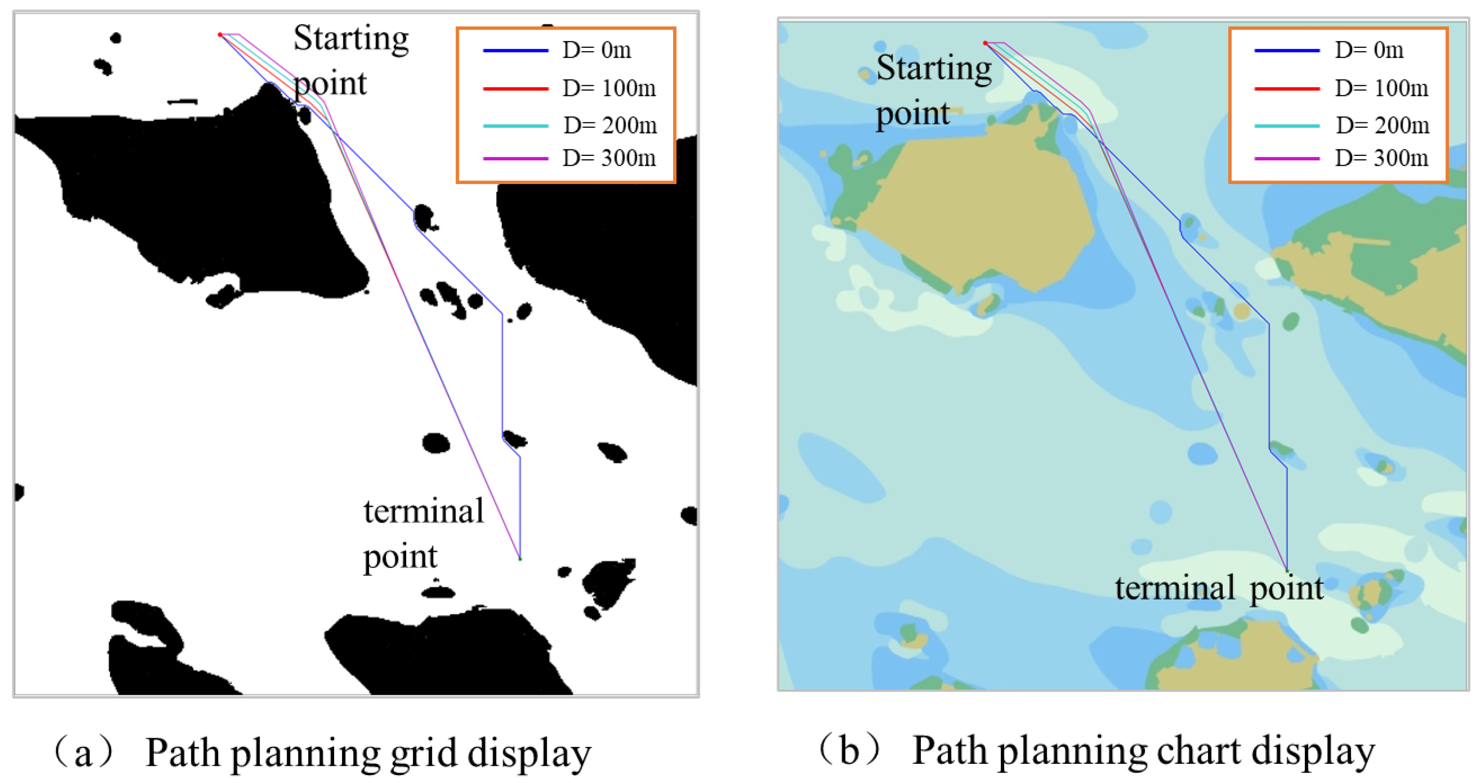
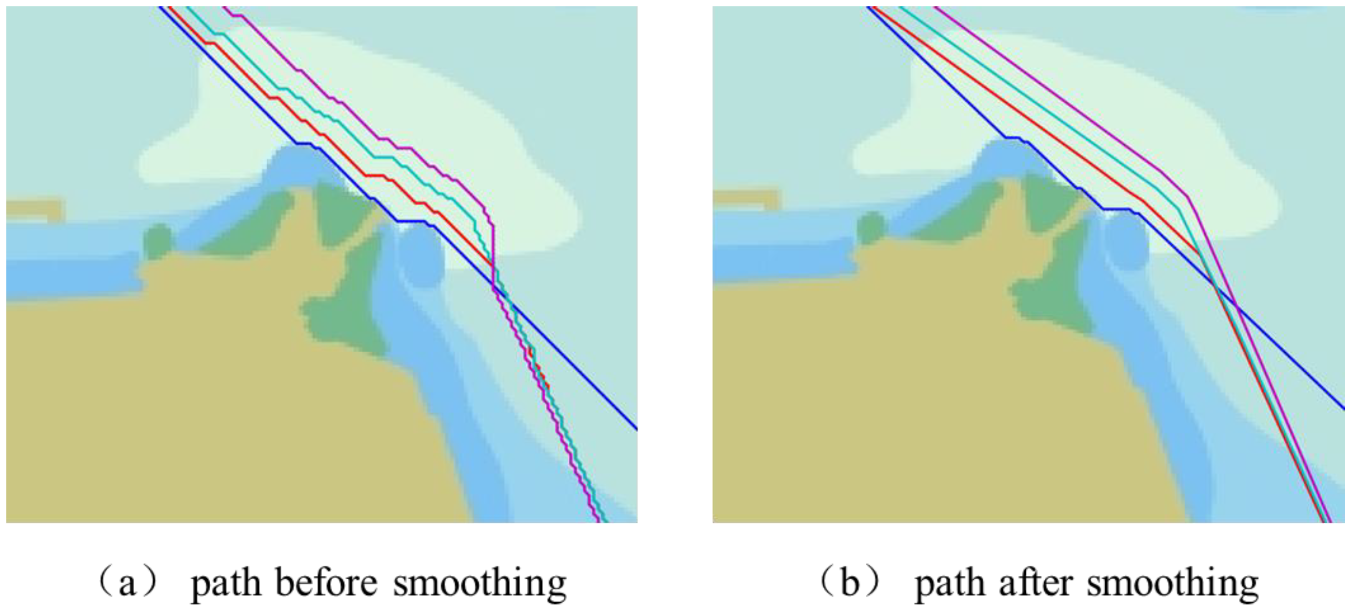
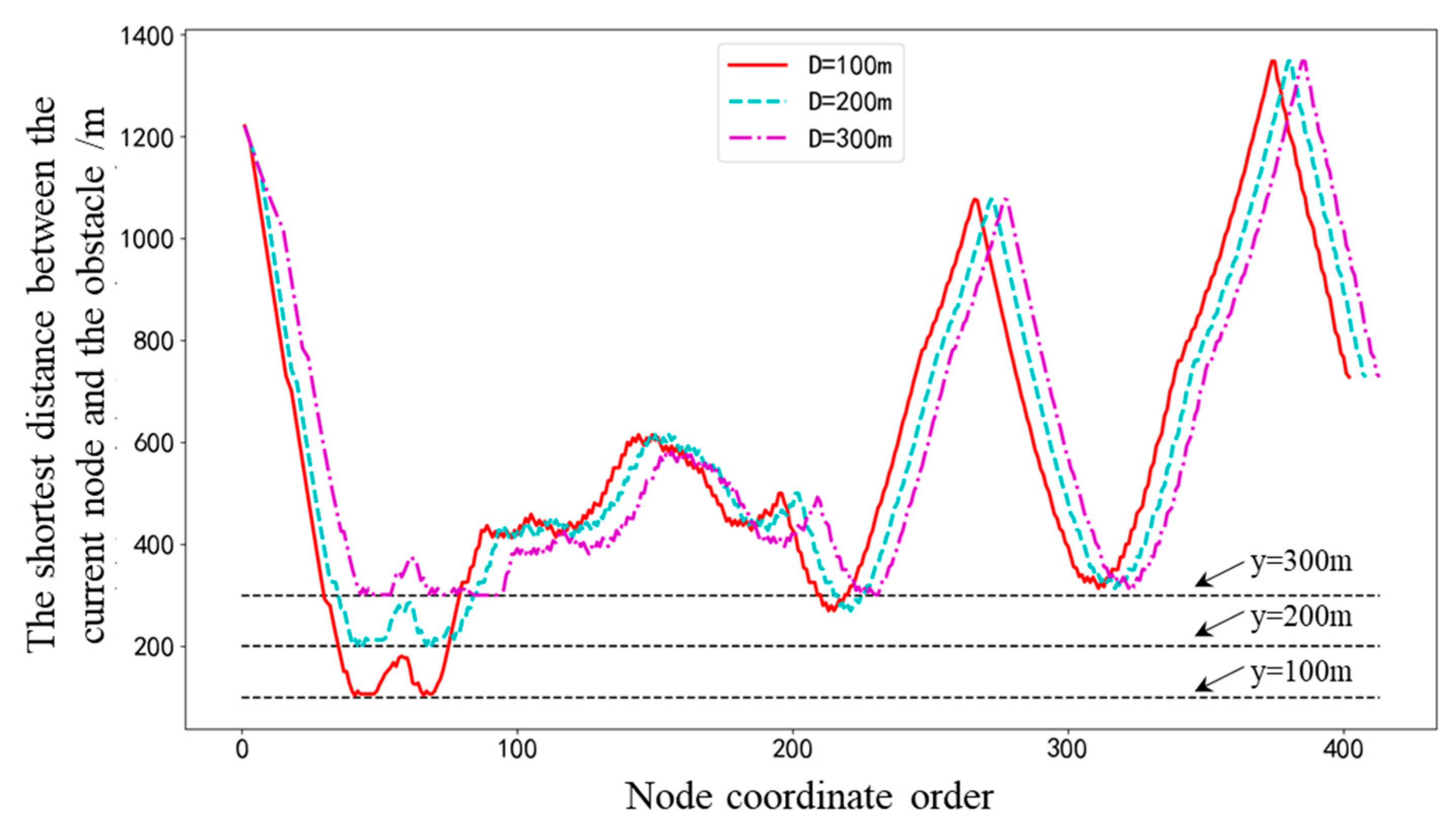
4.1. Experimental Results of Global Path Planning
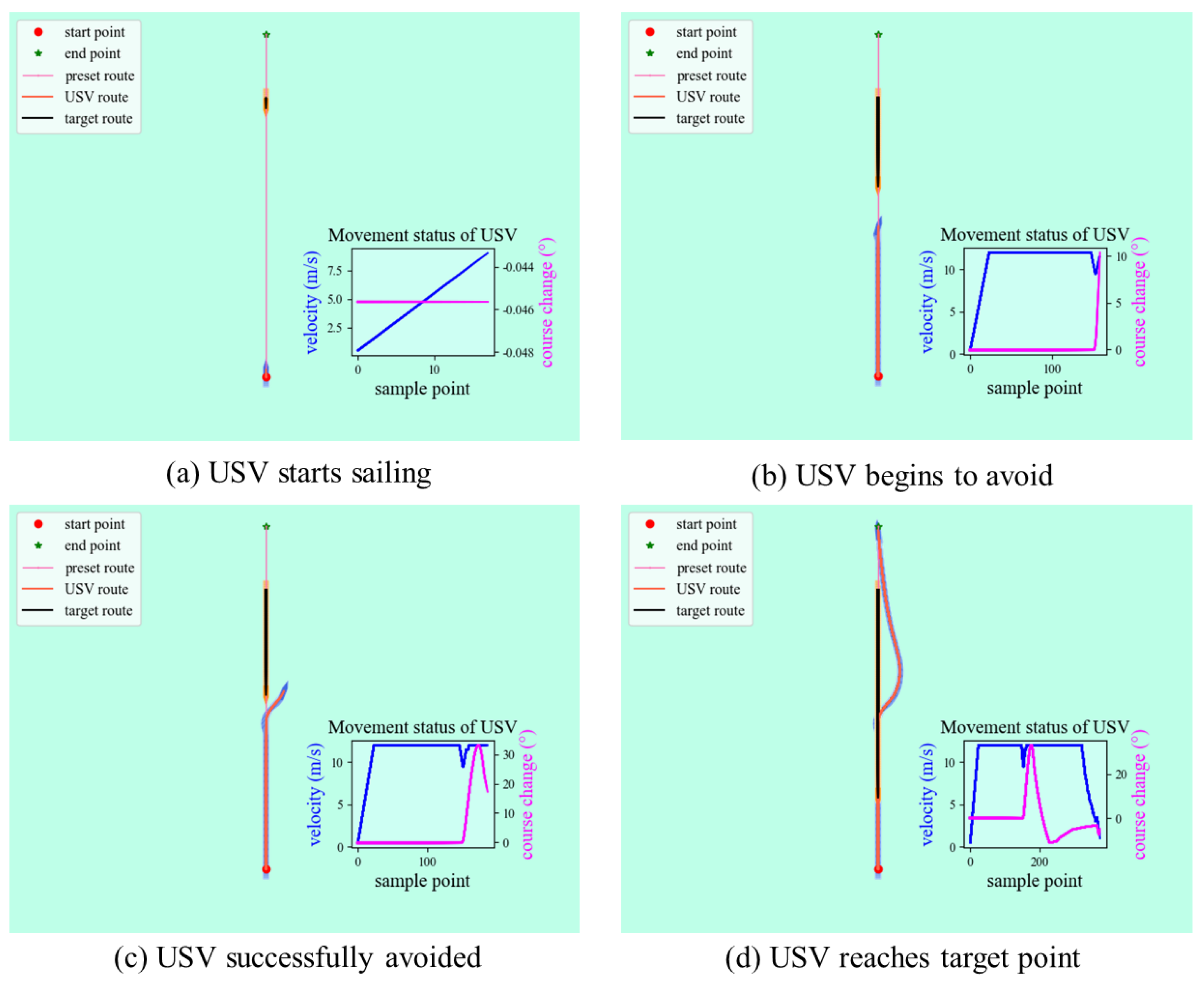
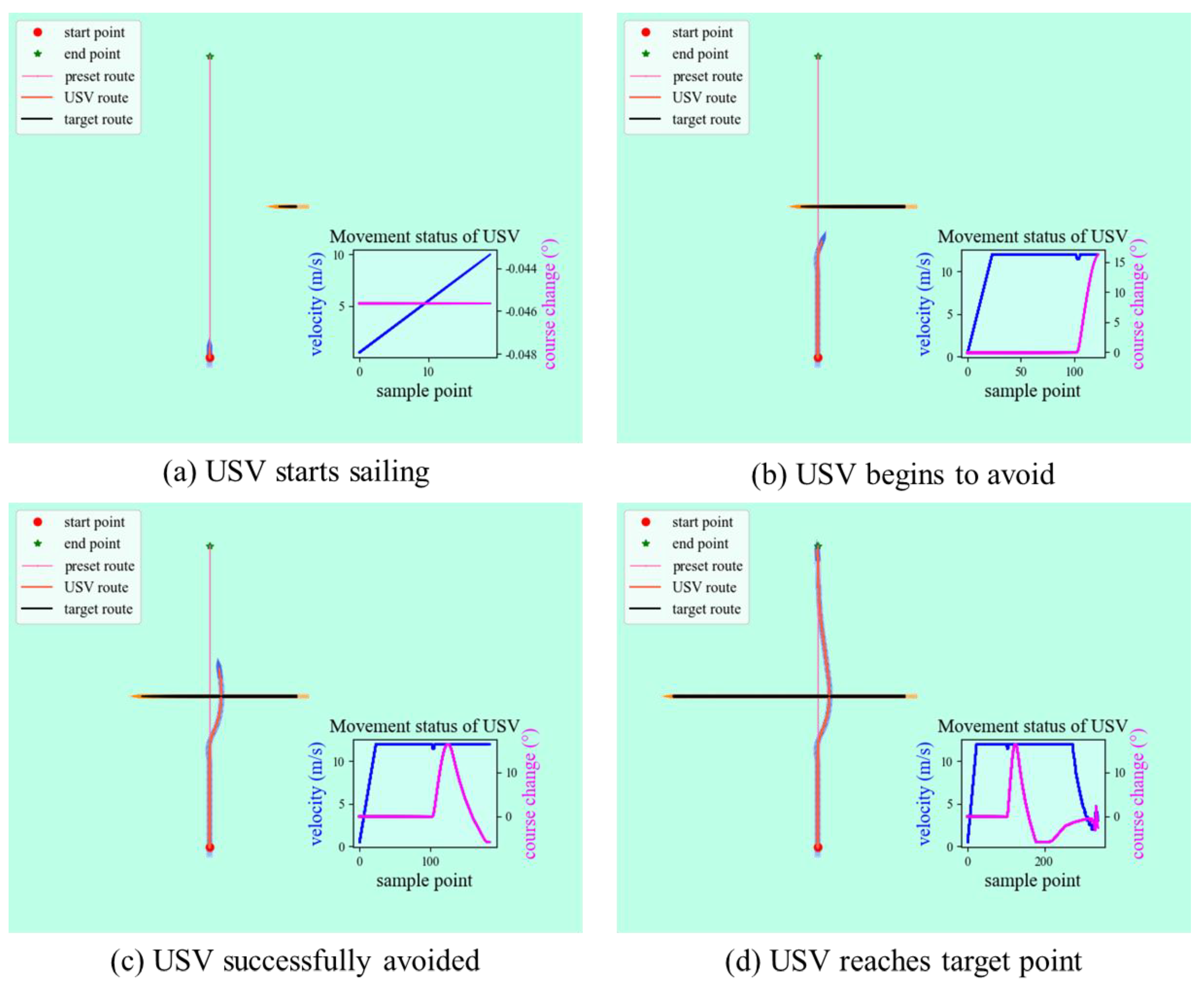
4.2. Experimental Simulation under Different Encounter Situations
- (1)
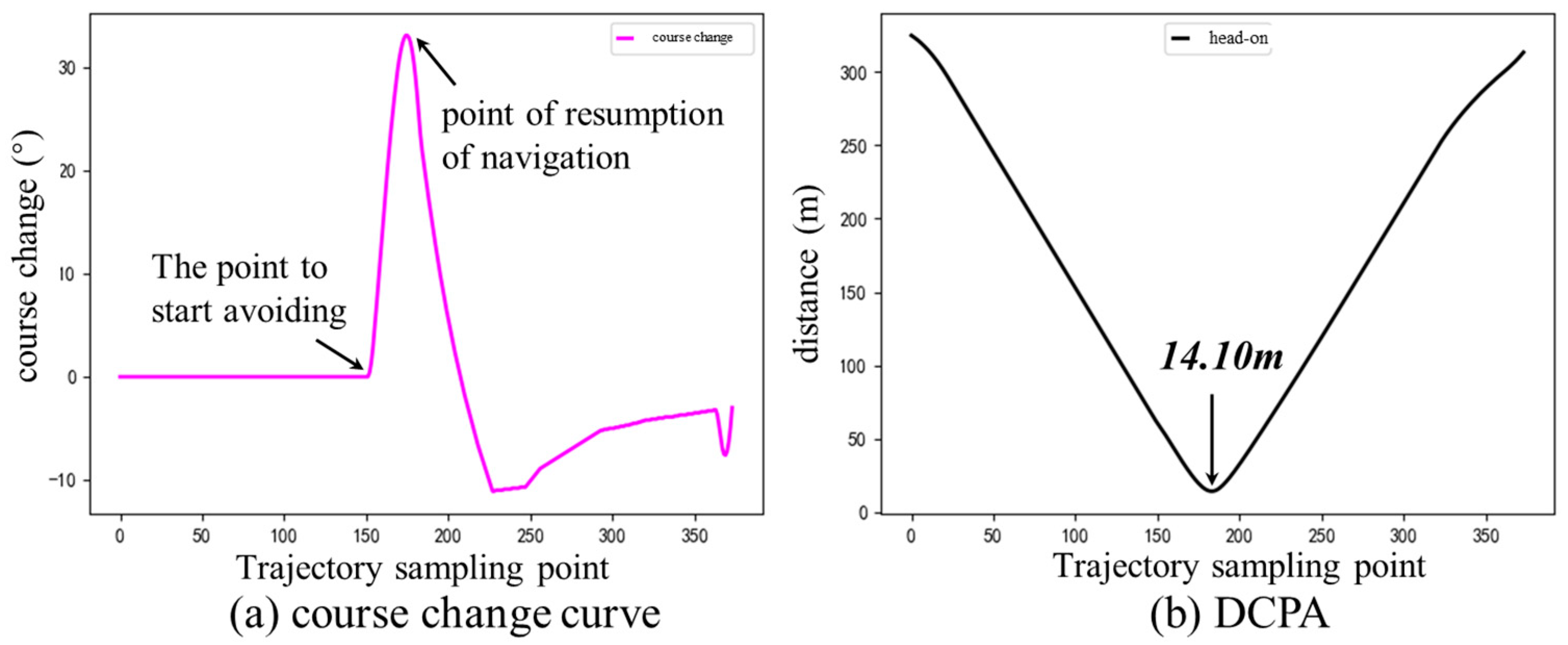
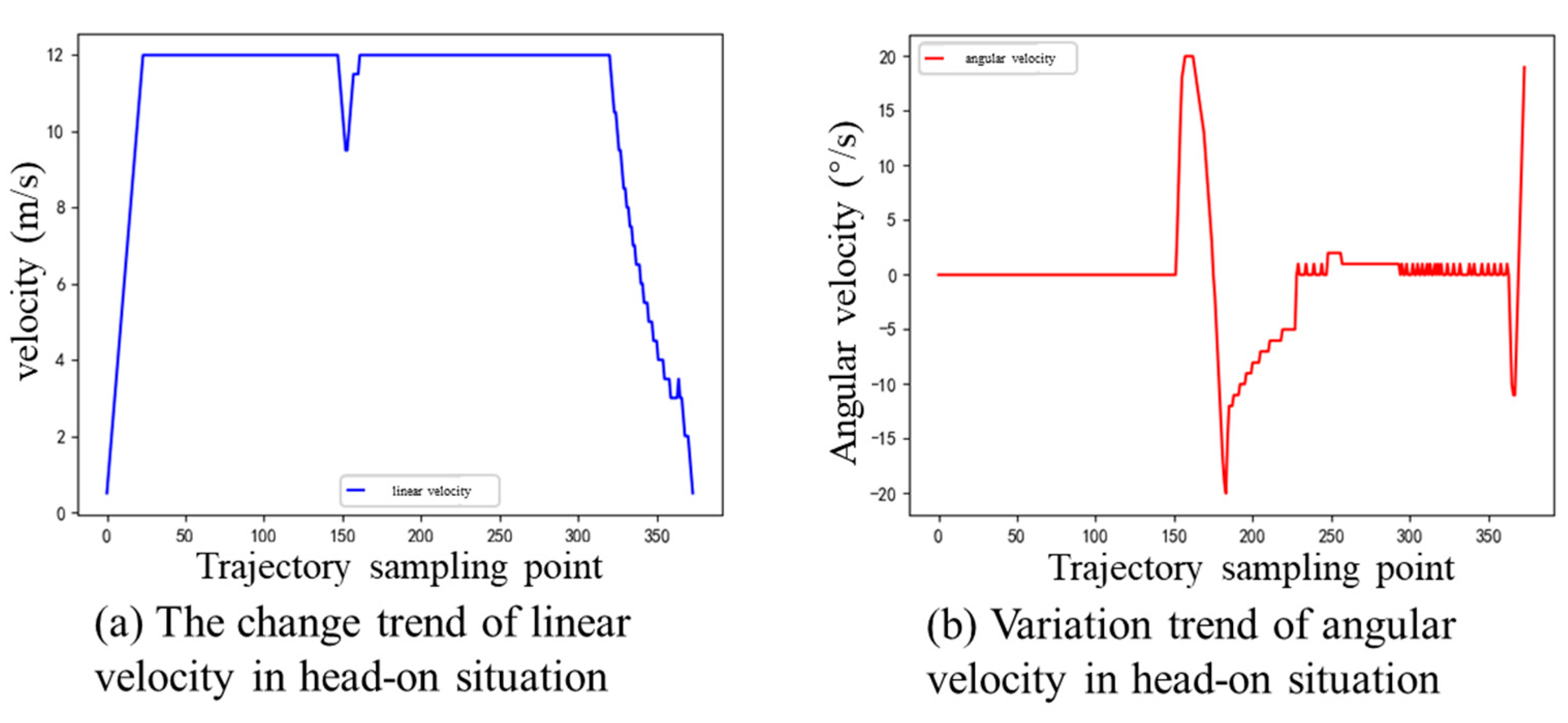
- Head-on situation
- (2)
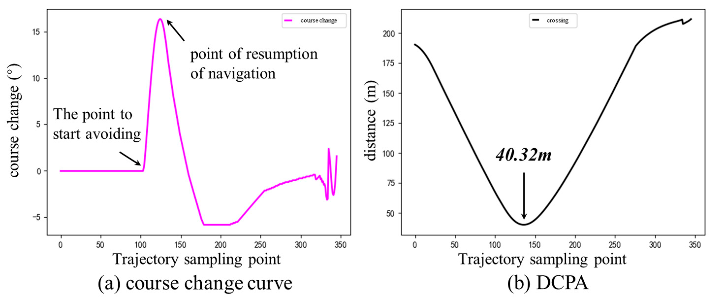
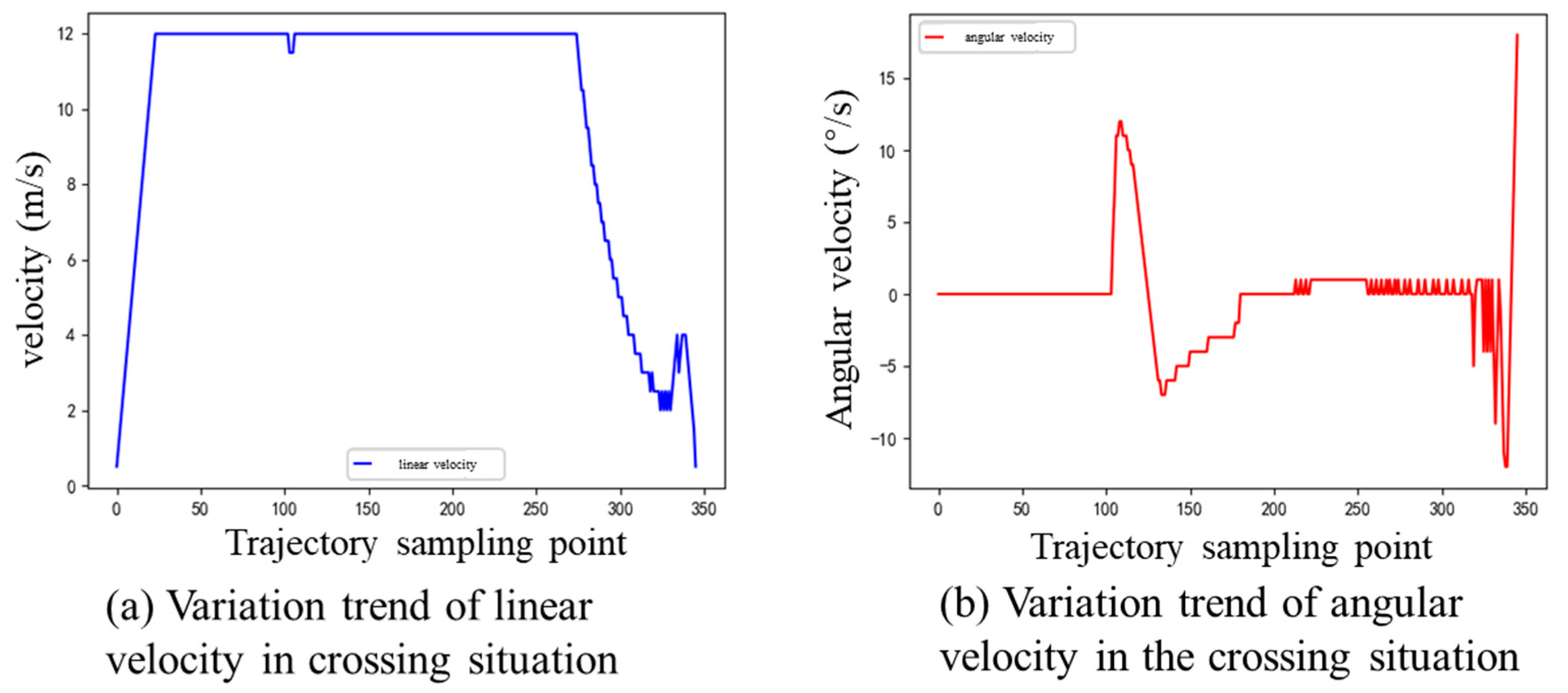
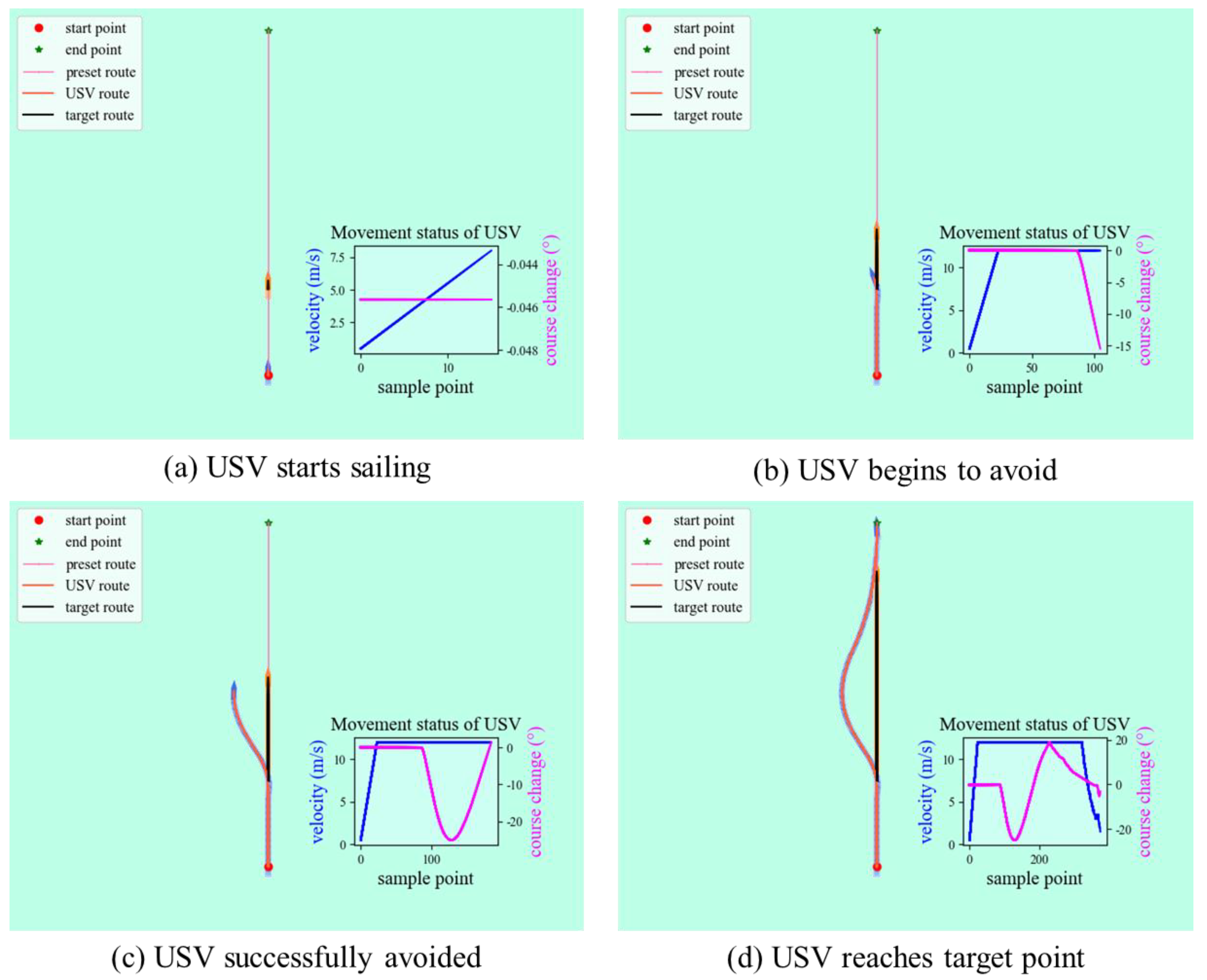
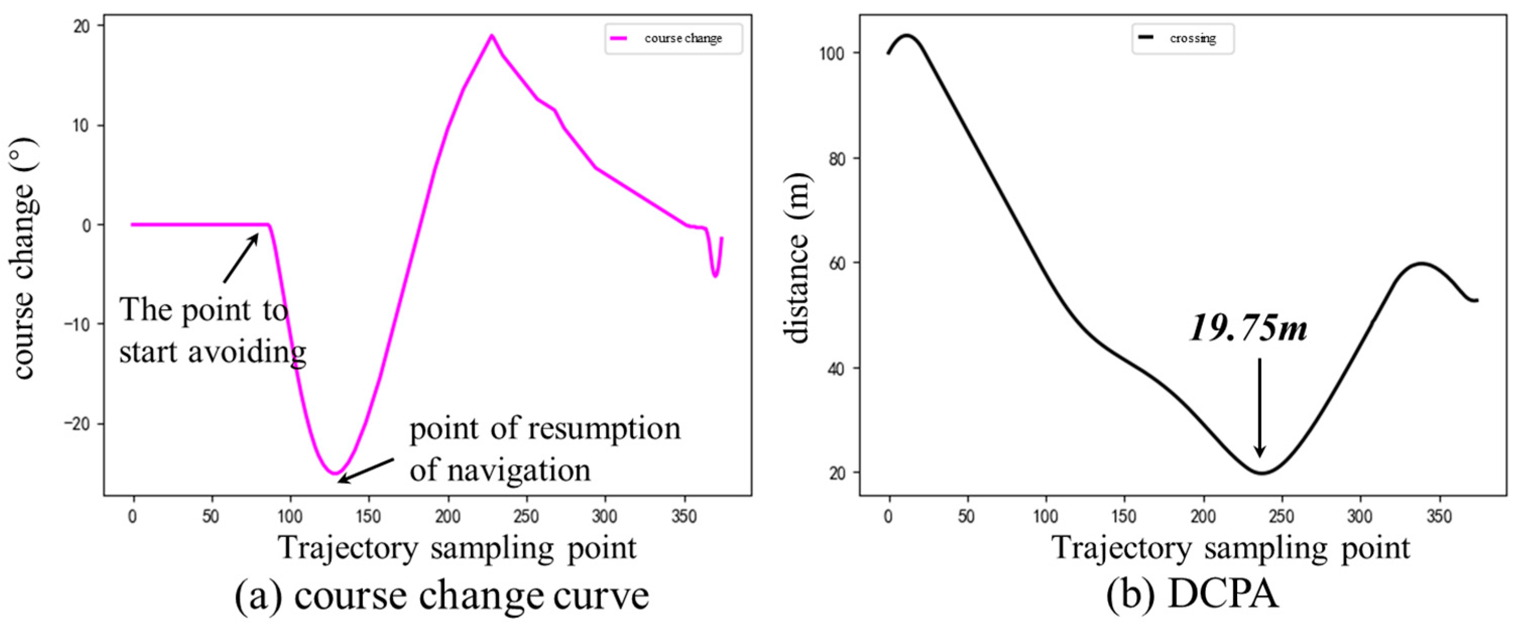
- Crossing situation
- (3)
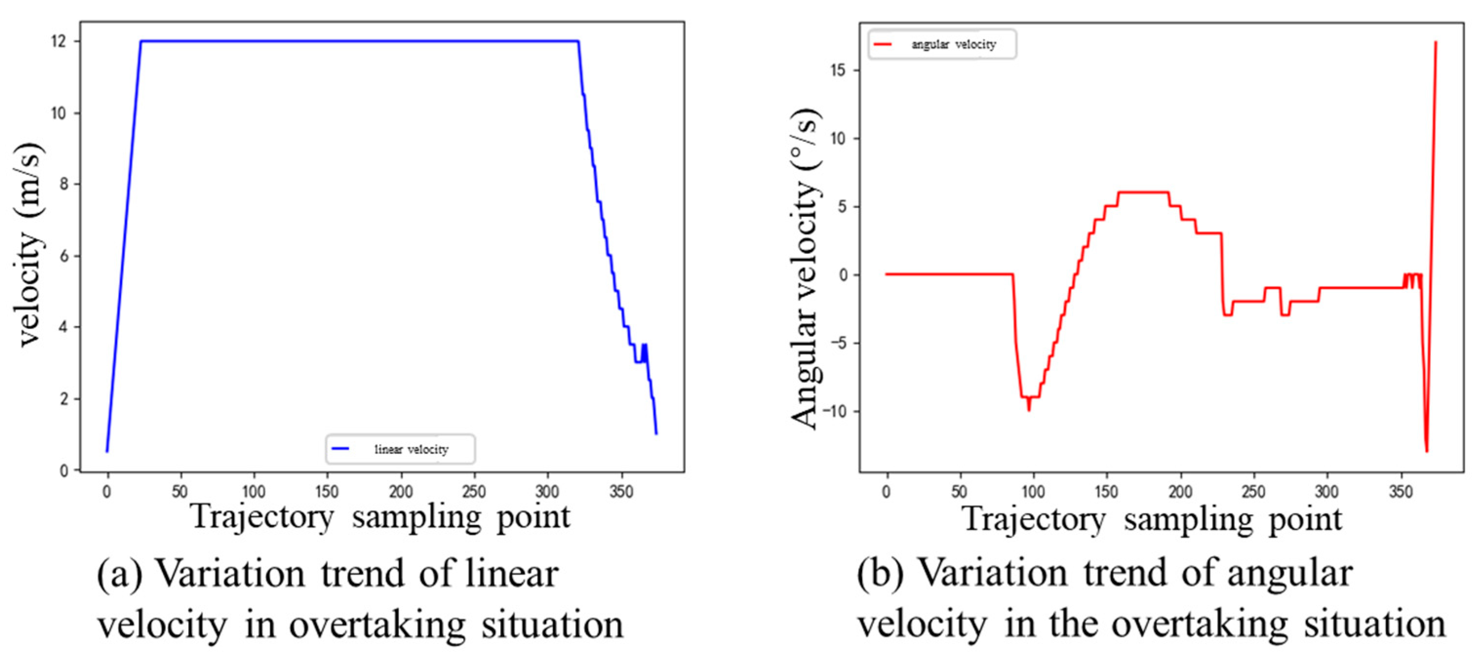
- Overtaking situation
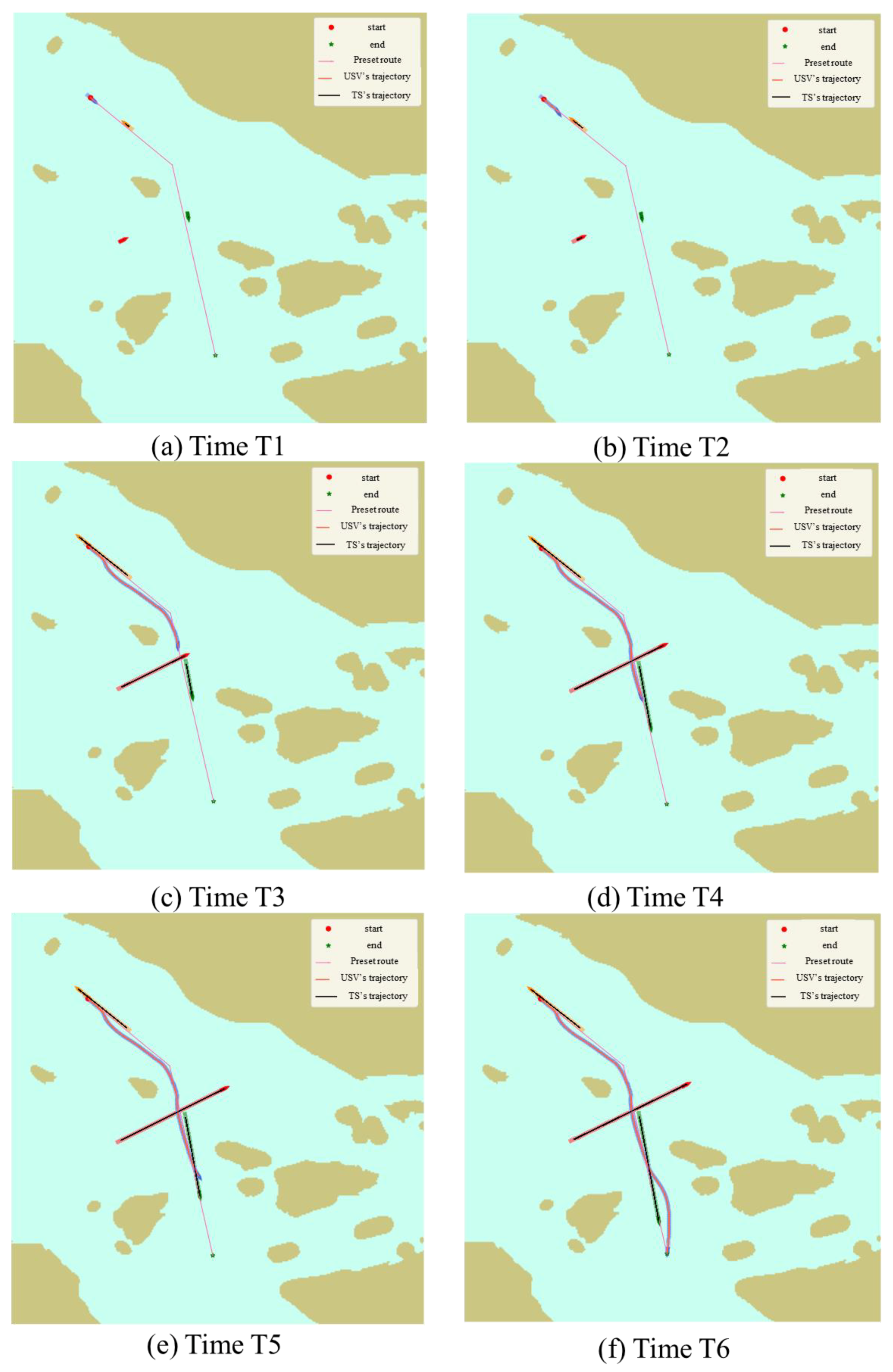
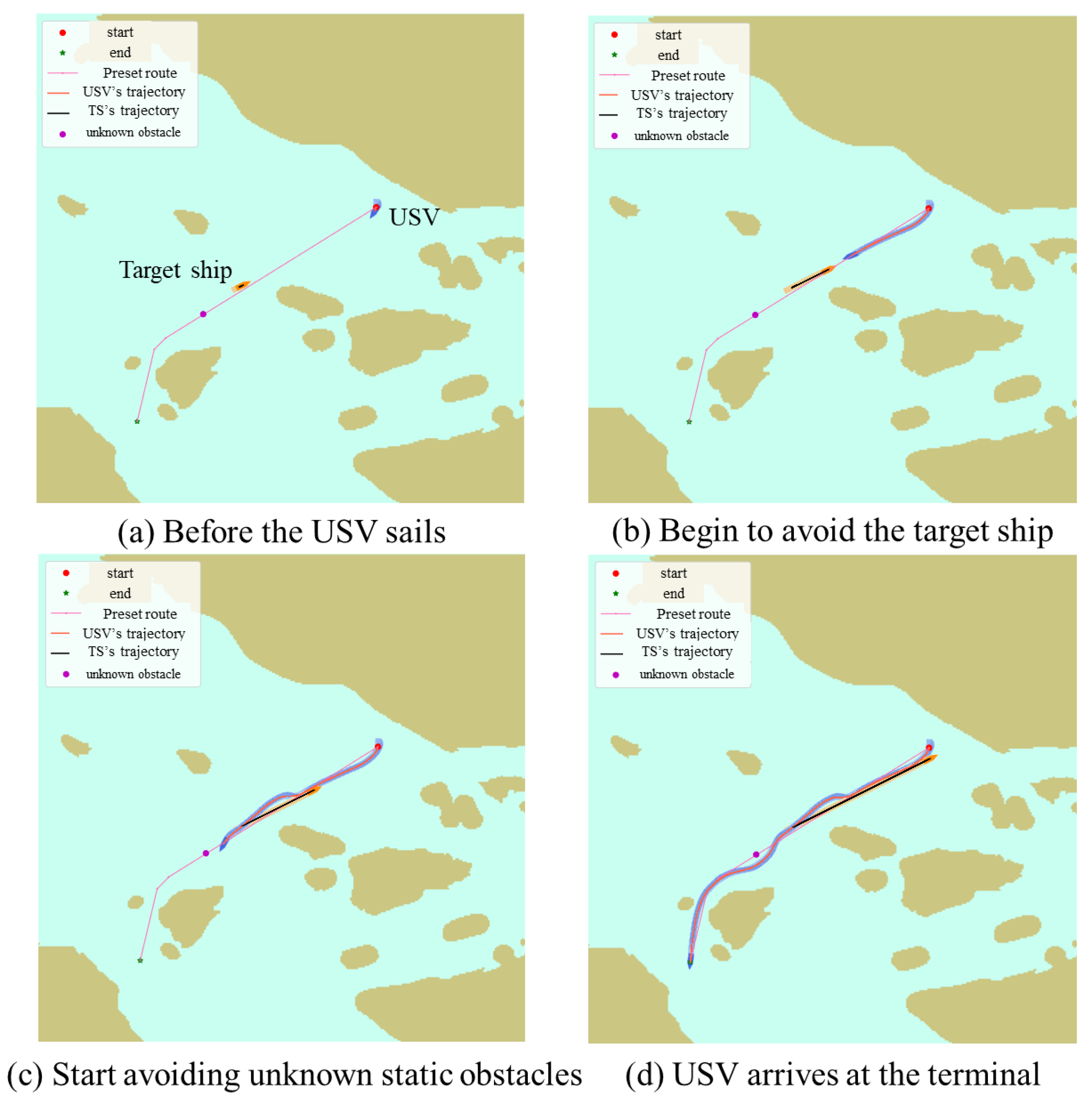
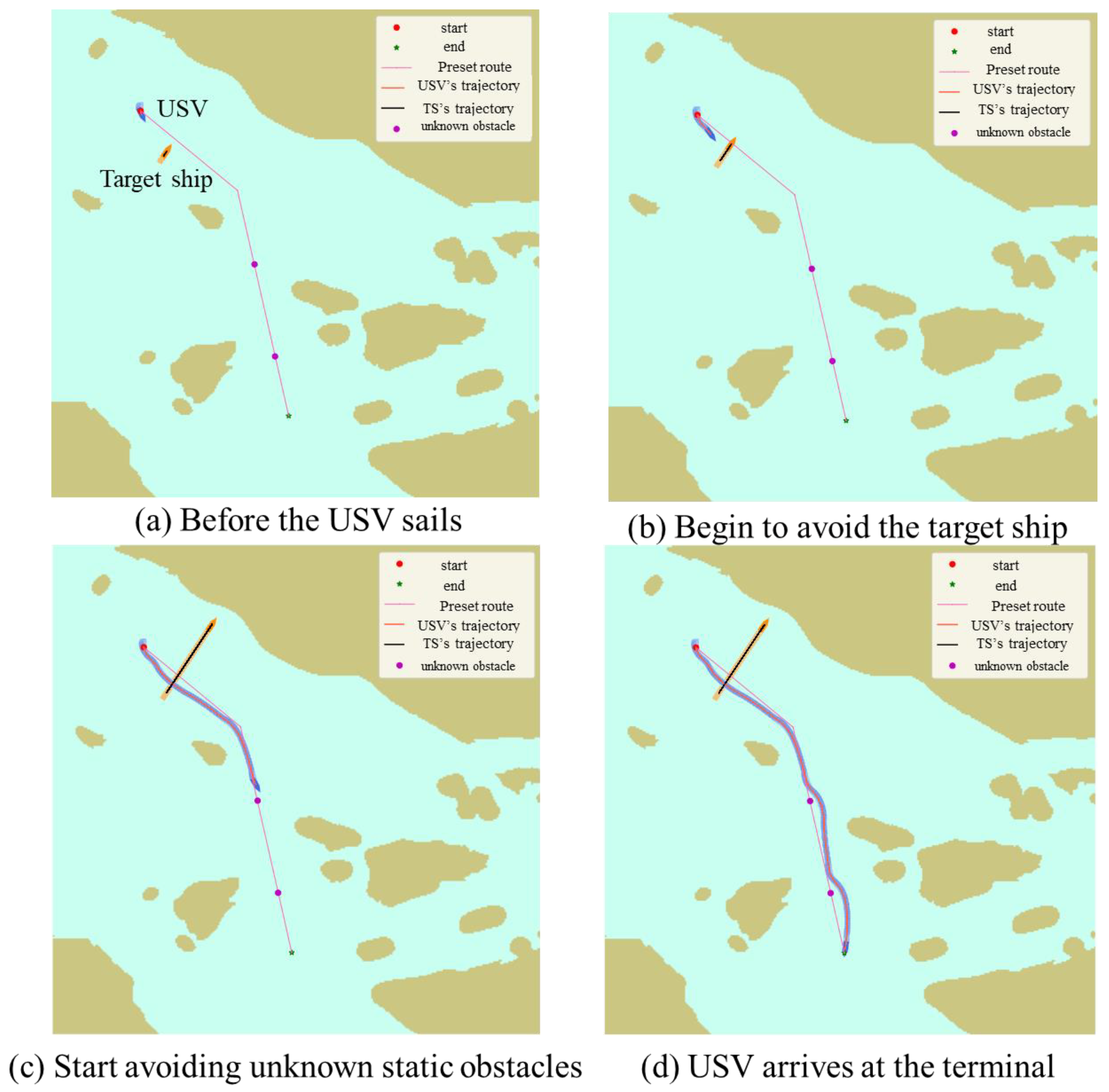
4.3. Experimental Simulation in a Local Environment
- (1)
- Local path planning with dynamic obstructing ships and unknown static obstacles in the head-on situation.
- (2)
- Local path planning with dynamic obstructing ships and unknown static obstacles in crossing situations.
- (3)
- Local path planning in the overtaking situation with dynamic obstructing ships and unknown static obstacles.
- (4)
- Local path planning in three different situations containing dynamic obstructing ships and unknown static obstacles.
5. Conclusions
Author Contributions
Funding
Institutional Review Board Statement
Informed Consent Statement
Data Availability Statement
Conflicts of Interest
References
- Long, Y.; Liu, S.; Qiu, D.; Li, C.; Guo, X.; Shi, B.; AbouOmar, M.S. Local Path Planning with Multiple Constraints for USV Based on Improved Bacterial Foraging Optimization Algorithm. J. Mar. Sci. Eng. 2023, 11, 489. [Google Scholar] [CrossRef]
- Liu, X.; Li, Y.; Zhang, J.; Zheng, J.; Yang, C. Self-Adaptive Dynamic Obstacle Avoidance and Path Planning for USV under Complex Maritime Environment. IEEE Access 2019, 7, 114945–114954. [Google Scholar] [CrossRef]
- Liu, J.; Yan, X.; Liu, C.; Fan, A.; Ma, F. Developments and Applications of Green and Intelligent Inland Vessels in China. J. Mar. Sci. Eng. 2023, 11, 318. [Google Scholar] [CrossRef]
- Song, R.; Liu, Y.; Bucknall, R. Smoothed A* Algorithm for Practical Unmanned Surface Vehicle Path Planning. Appl. Ocean Res. 2019, 83, 9–20. [Google Scholar] [CrossRef]
- Han, X.; Zhang, X.; Zhang, H. Trajectory Planning of USV: On-Line Computation of the Double S Trajectory Based on Multi-Scale A* Algorithm with Reeds–Shepp Curves. J. Mar. Sci. Eng. 2023, 11, 153. [Google Scholar] [CrossRef]
- Zhao, J.; Yan, Z.; Chen, X.; Han, B.; Wu, S.; Ke, R. k-GCN-LSTM: A k-hop Graph Convolutional Network and Long–Short-Term Memory for ship speed prediction. Physica A 2022, 606, 128107. [Google Scholar] [CrossRef]
- Feng, Z.; Pan, Z.; Chen, W.; Liu, Y.; Leng, J. USV Application Scenario Expansion Based on Motion Control, Path Following and Velocity Planning. Machines 2022, 10, 310. [Google Scholar] [CrossRef]
- Xu, P.F.; Ding, Y.X.; Luo, J.C. Complete Coverage Path Planning of an Unmanned Surface Vehicle Based on a Complete Coverage Neural Network Algorithm. J. Mar. Sci. Eng. 2021, 9, 1163. [Google Scholar] [CrossRef]
- Ke, C.; Chen, H. Cooperative Path Planning for Air–Sea Heterogeneous Unmanned Vehicles Using Search-and-Tracking Mission. Ocean Eng. 2022, 262, 112020. [Google Scholar] [CrossRef]
- Zhang, J.; Zhang, D.; Yan, X.; Haugen, S.; Soares, C.G. A distributed anti-collision decision support formulation in multi-ship encounter situations under COLREGs. Ocean Eng. 2015, 105, 336–348. [Google Scholar] [CrossRef]
- Cai, M.; Zhang, J.; Zhang, D.; Yuan, X.; Soares, C.G. Collision risk analysis on ferry ships in Jiangsu Section of the Yangtze River based on AIS data. J. Reliab. Eng. Syst. Saf. 2021, 215, 107901. [Google Scholar] [CrossRef]
- Xu, H.; Hinostroza, M.A.; Guedes Soares, C. Modified Vector Field Path-Following Control System for an underactuated Autonomous surface ship model in the presence of static obstacles. J. Mar. Sci. Eng. 2021, 9, 652. [Google Scholar] [CrossRef]
- Zhang, J.; Zhang, H.; Liu, J.; Wu, D.; Soares, C.G. A Two-Stage Path Planning Algorithm Based on Rapid-Exploring Random Tree for Ships Navigating in Multi-Obstacle Water Areas Considering COLREGs. J. Mar. Sci. Eng. 2022, 10, 1441. [Google Scholar] [CrossRef]
- Zhang, Y.; Shi, G.; Liu, J. Dynamic Energy-Efficient Path Planning of Unmanned Surface Vehicle under Time-Varying Current and Wind. J. Mar. Sci. Eng. 2022, 10, 759. [Google Scholar] [CrossRef]
- Almoaili, E.; Kurdi, H. Path Planning Algorithm for Unmanned Ground Vehicles (UGVs) in Known Static Environments. Procedia Comput. Sci. 2020, 177, 57–63. [Google Scholar] [CrossRef]
- Wang, H.; Lu, L.; Li, T.; Wang, A. Multi-AUG Three-Dimensional Path Planning and Secure Cooperative Path Following under DoS Attacks. Ocean Eng. 2023, 274, 113864. [Google Scholar] [CrossRef]
- Jabbarpour, M.R.; Zarrabi, H.; Jung, J.J.; Kim, P. A Green Ant-Based Method for Path Planning of Unmanned Ground Vehicles. IEEE Access 2017, 5, 1820–1832. [Google Scholar] [CrossRef]
- Han, Z.; Chen, M.; Shao, S.; Wu, Q. Improved Artificial Bee Colony Algorithm-Based Path Planning of Unmanned Autonomous Helicopter Using Multi-Strategy Evolutionary Learning. Aerosp. Sci. Technol. 2022, 122, 107374. [Google Scholar] [CrossRef]
- Thoresen, M.; Nielsen, N.H.; Mathiassen, K.; Pettersen, K.Y. Path Planning for UGVs Based on Traversability Hybrid A*. IEEE Robot. Autom. Lett. 2021, 6, 1216–1223. [Google Scholar] [CrossRef]
- Shin, J.; Kwak, D.; Kwak, K. Model Predictive Path Planning for an Autonomous Ground Vehicle in Rough Terrain. Int. J. Control. Autom. Syst. 2021, 19, 2224–2237. [Google Scholar] [CrossRef]
- Chen, D.; Wang, Z.; Zhou, G.; Li, S. Path Planning and Energy Efficiency of Heterogeneous Mobile Robots Using Cuckoo–Beetle Swarm Search Algorithms with Applications in UGV Obstacle Avoidance. Sustainability 2022, 14, 15137. [Google Scholar] [CrossRef]
- Liang, C.; Zhang, X.; Watanabe, Y.; Deng, Y. Autonomous Collision Avoidance of Unmanned Surface Vehicles Based on Improved A Star And Minimum Course Alteration Algorithms. Appl. Ocean Res. 2021, 113, 102755. [Google Scholar] [CrossRef]
- Pasandi, L.; Hooshmand, M.; Rahbar, M. Modified A* Algorithm Integrated with Ant Colony Optimization for Multi-Objective Route-Finding; Case Study: Yazd. Appl. Soft Comput. 2021, 113, 107877. [Google Scholar] [CrossRef]
- Li, J.; Zhang, W.; Hu, Y.; Fu, S.; Liao, C.; Yu, W. RJA-Star Algorithm for UAV Path Planning Based on Improved R5DOS Model. Appl. Sci. 2023, 13, 1105. [Google Scholar] [CrossRef]
- Zou, A.; Wang, L.; Li, W.; Cai, J.; Wang, H.; Tan, T. Mobile Robot Path Planning Using Improved Mayfly Optimization Algorithm and Dynamic Window Approach. J. Supercomput. 2022, 79, 8340–8367. [Google Scholar] [CrossRef]
- Wang, N.; Xu, H. Dynamics-Constrained Global-Local Hybrid Path Planning of an Autonomous Surface Vehicle. IEEE Trans. Veh. Technol. 2020, 69, 6928–6942. [Google Scholar] [CrossRef]
- Han, S.; Wang, L.; Wang, Y.; He, H. A Dynamically Hybrid Path Planning for Unmanned Surface Vehicles Based on Non-Uniform Theta* and Improved Dynamic Windows Approach. Ocean Eng. 2022, 257, 111655. [Google Scholar] [CrossRef]
- Ji, X.; Feng, S.; Han, Q.; Yin, H.; Yu, S. Improvement and Fusion of A* Algorithm and Dynamic Window Approach Considering Complex Environmental Information. Arab. J. Sci. Eng. 2021, 46, 7445–7459. [Google Scholar] [CrossRef]
- Chi, W.; Ding, Z.; Wang, J.; Chen, G.; Sun, L. A Generalized Voronoi Diagram-Based Efficient Heuristic Path Planning Method for RRTs in Mobile Robots. IEEE Trans. Ind. Electron. 2022, 69, 4926–4937. [Google Scholar] [CrossRef]
- Chi, W.; Wang, J.; Ding, Z.; Chen, G.; Sun, L. A Reusable Generalized Voronoi Diagram-Based Feature Tree for Fast Robot Motion Planning in Trapped Environments. IEEE Sens. J. 2022, 22, 17615–17624. [Google Scholar] [CrossRef]
- Schoener, M.; Coyle, E.; Thompson, D. An Anytime Visibility–Voronoi Graph-Search Algorithm for Generating Robust and Feasible Unmanned Surface Vehicle Paths. Auton. Robots 2022, 46, 911–927. [Google Scholar] [CrossRef]


| Chart Environmental Information | Color | Red | Green | Blue |
|---|---|---|---|---|
| Areas with a water depth of 30–50 m |  | 216 | 244 | 225 |
| Areas with a water depth of 10–20 m |  | 185 | 225 | 222 |
| Areas with a water depth of 5 m |  | 152 | 211 | 237 |
| Areas with a water depth of 1–2 m |  | 123 | 193 | 241 |
| shoal |  | 115 | 185 | 142 |
| land |  | 203 | 199 | 131 |
| Safe Distance/m | Original Path Length/km | Optimized Path Length/km | Number of Nodes | Number of Optimized Nodes |
|---|---|---|---|---|
| D = 0 | 12.08 | - | 398 | - |
| D = 100 | 12.14 | 11.32 | 402 | 5 |
| D = 200 | 12.23 | 11.38 | 409 | 6 |
| D = 300 | 12.30 | 11.48 | 414 | 6 |
| Parameter | Linear Velocity | Angular Velocity |
|---|---|---|
| minimum value | 0 m/s | −20°/s |
| maximum value | 5 m/s | 20°/s |
| maximum acceleration | 2 m/s2 | 5°/s2 |
| sampling interval | 0.2 m/s | 1°/s |
| Predicted Time/s | Safe Distance/m | ||||
|---|---|---|---|---|---|
| 0.02 | 0.4 | 0.2 | 0.2 | 5 | 50 |
Disclaimer/Publisher’s Note: The statements, opinions and data contained in all publications are solely those of the individual author(s) and contributor(s) and not of MDPI and/or the editor(s). MDPI and/or the editor(s) disclaim responsibility for any injury to people or property resulting from any ideas, methods, instructions or products referred to in the content. |
© 2023 by the authors. Licensee MDPI, Basel, Switzerland. This article is an open access article distributed under the terms and conditions of the Creative Commons Attribution (CC BY) license (https://creativecommons.org/licenses/by/4.0/).
Share and Cite
Hu, S.; Tian, S.; Zhao, J.; Shen, R. Path Planning of an Unmanned Surface Vessel Based on the Improved A-Star and Dynamic Window Method. J. Mar. Sci. Eng. 2023, 11, 1060. https://doi.org/10.3390/jmse11051060
Hu S, Tian S, Zhao J, Shen R. Path Planning of an Unmanned Surface Vessel Based on the Improved A-Star and Dynamic Window Method. Journal of Marine Science and Engineering. 2023; 11(5):1060. https://doi.org/10.3390/jmse11051060
Chicago/Turabian StyleHu, Shunan, Shenpeng Tian, Jiansen Zhao, and Ruiqi Shen. 2023. "Path Planning of an Unmanned Surface Vessel Based on the Improved A-Star and Dynamic Window Method" Journal of Marine Science and Engineering 11, no. 5: 1060. https://doi.org/10.3390/jmse11051060
APA StyleHu, S., Tian, S., Zhao, J., & Shen, R. (2023). Path Planning of an Unmanned Surface Vessel Based on the Improved A-Star and Dynamic Window Method. Journal of Marine Science and Engineering, 11(5), 1060. https://doi.org/10.3390/jmse11051060